Investigation of Pre-Earthquake Ionospheric and Atmospheric Disturbances for Three Large Earthquakes in Mexico


 ,
,  , ,
, ,  and
and
Abstract
1. Introduction
2. Materials and Methods
3. Results
3.1. Ionospheric Analysis
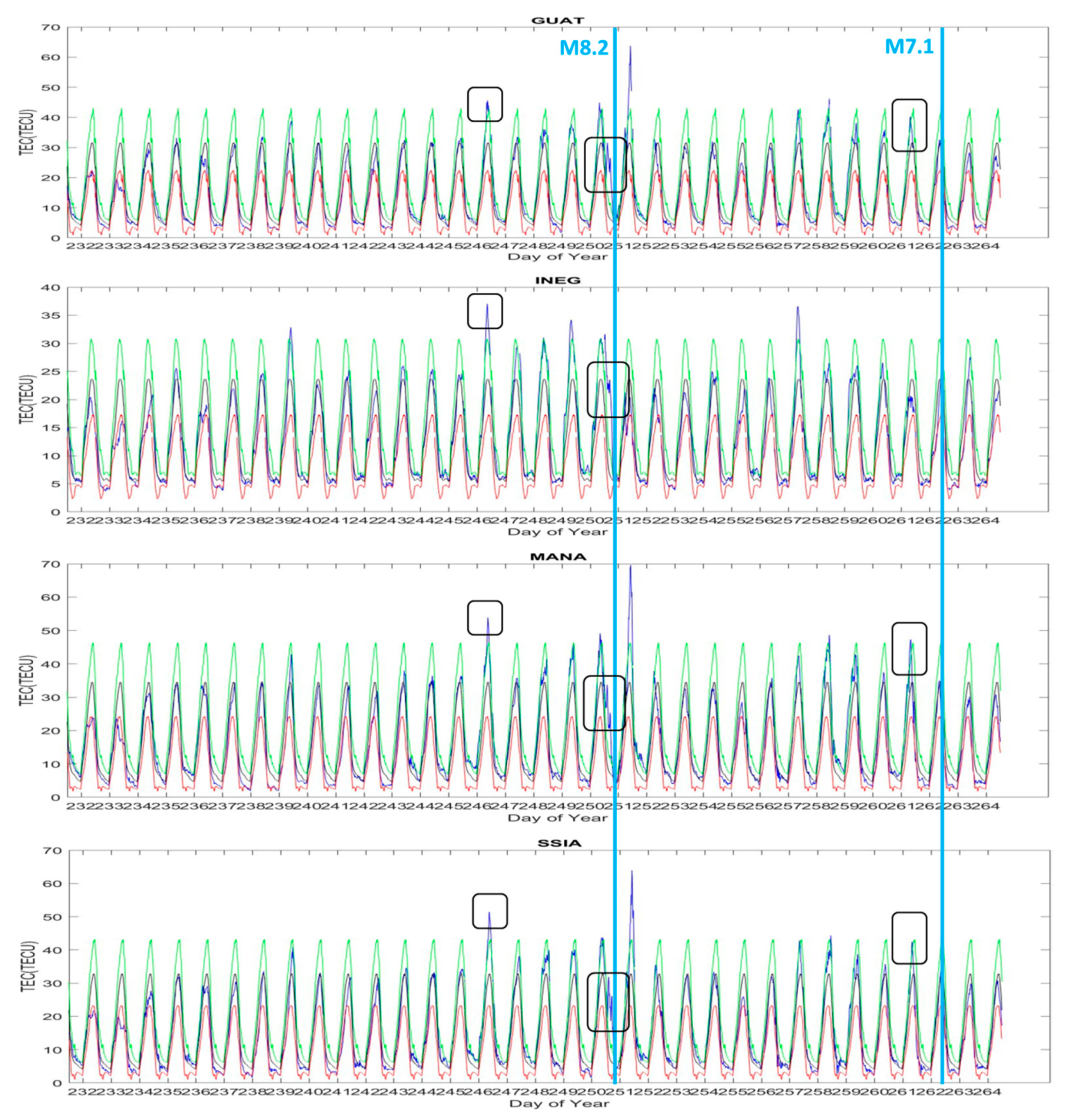
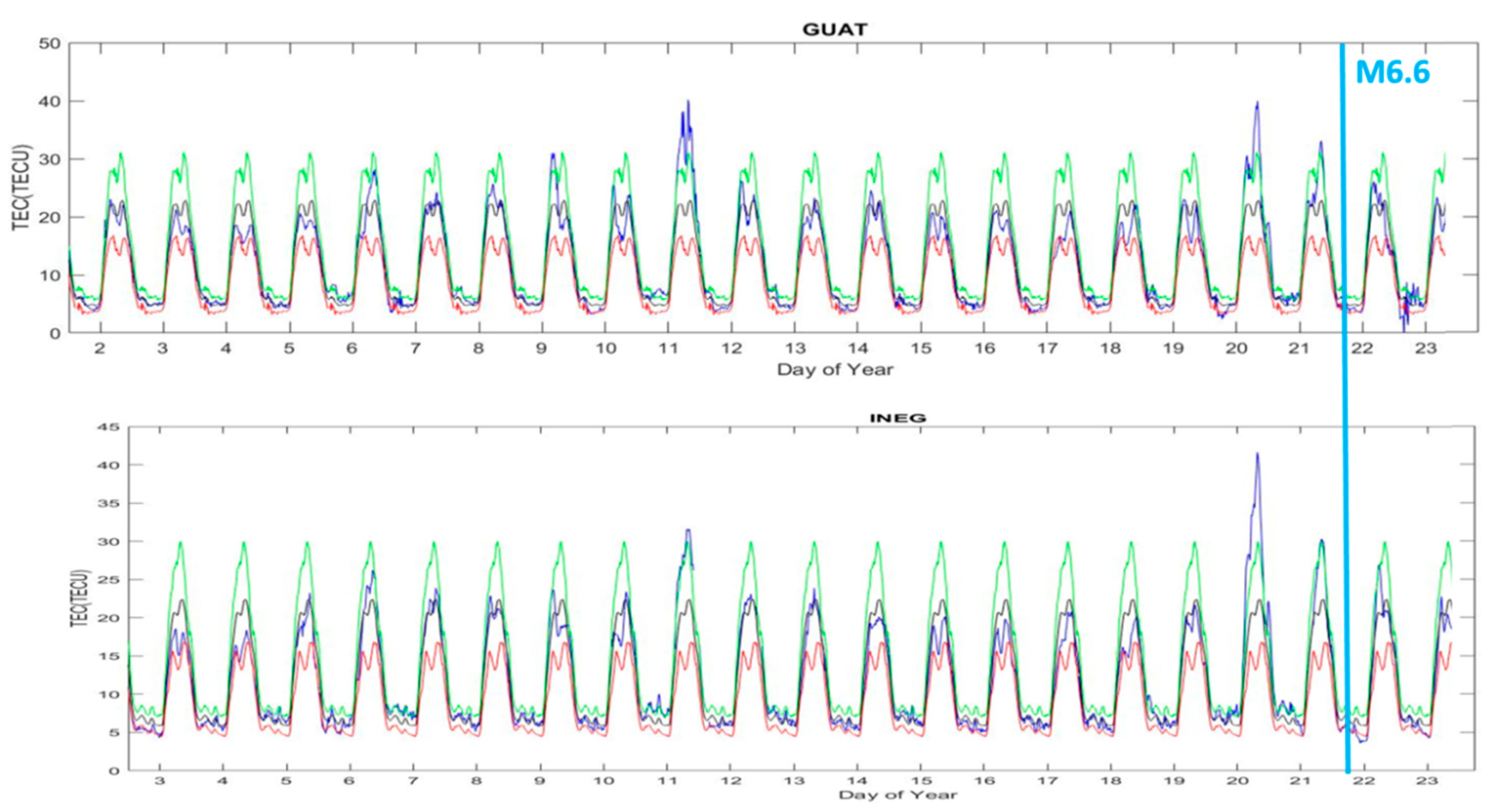
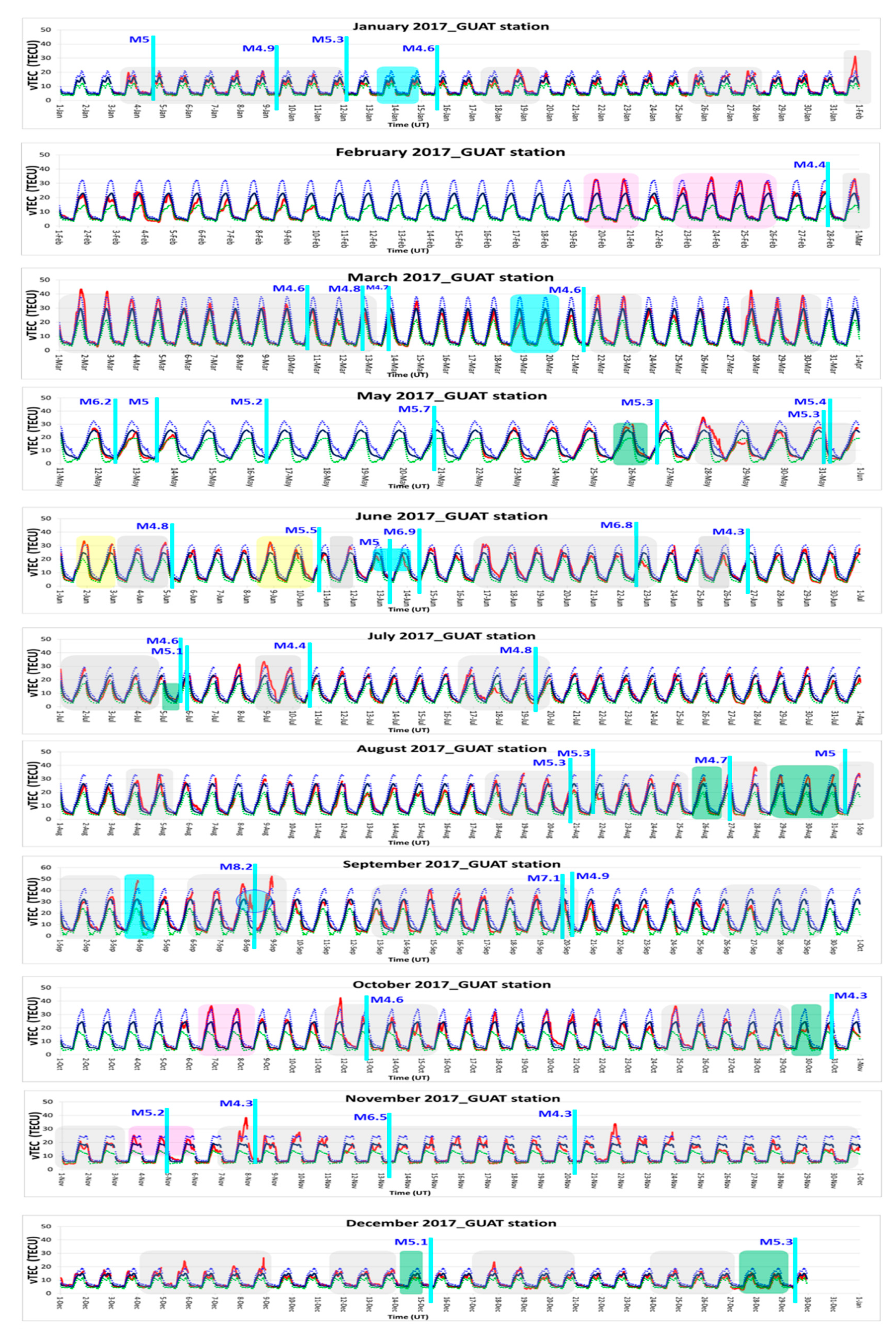
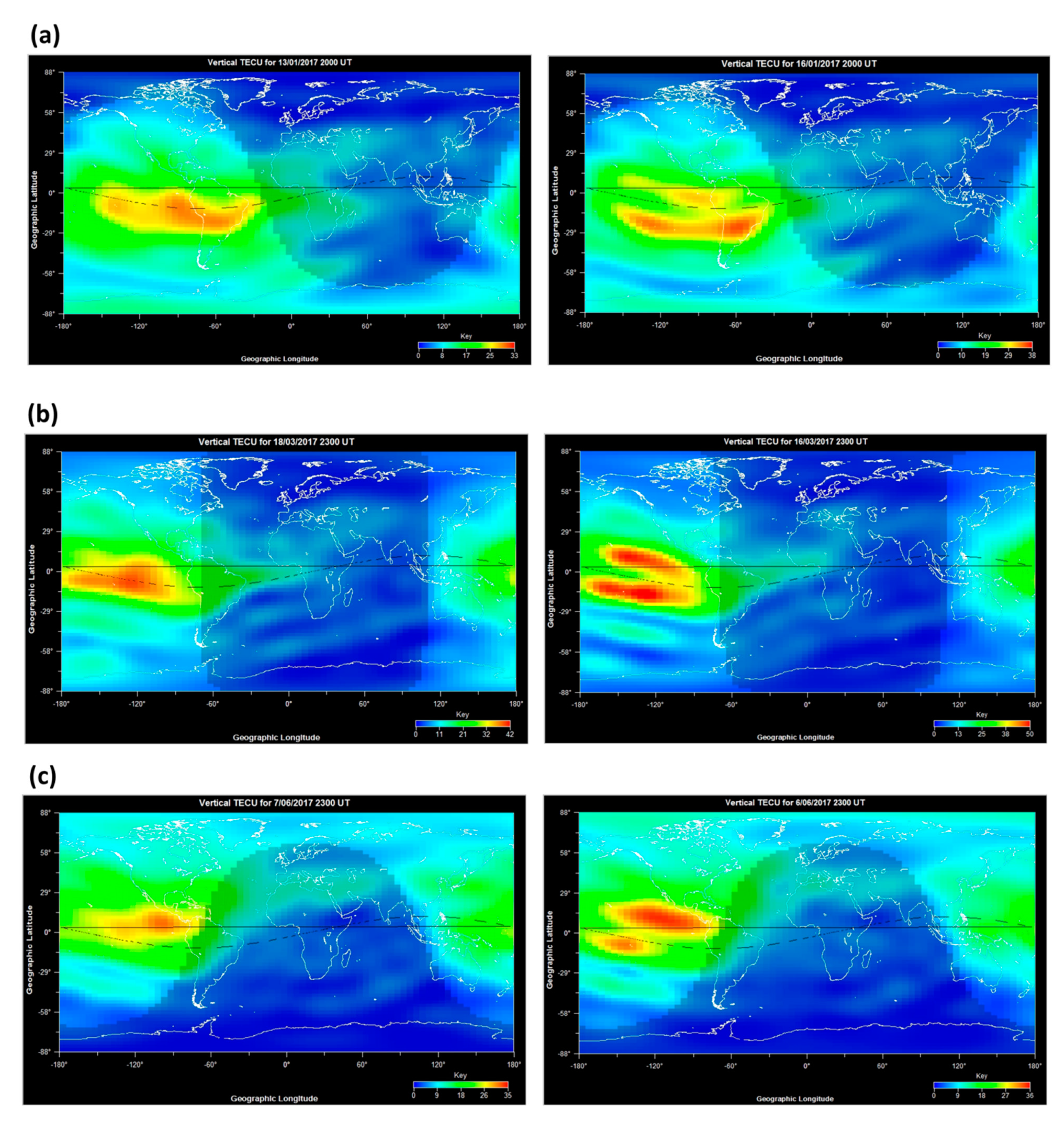
3.1.1. Statistical Analysis on Ionospheric TEC
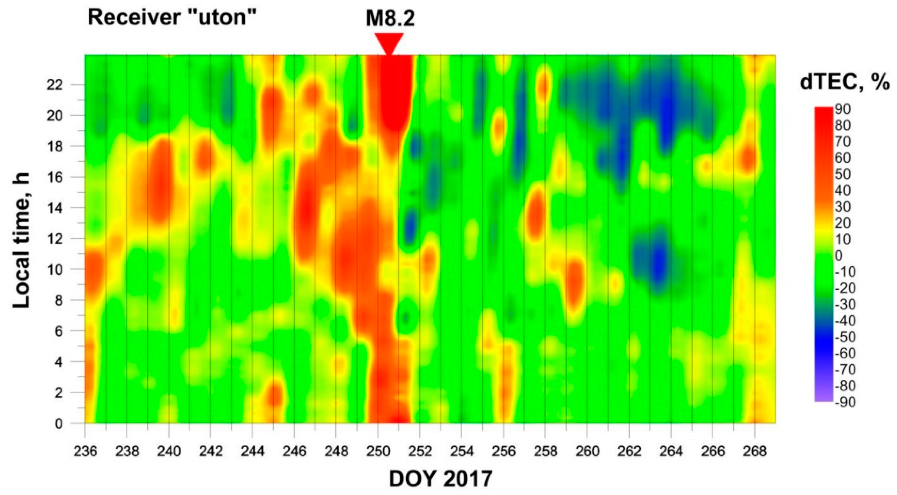
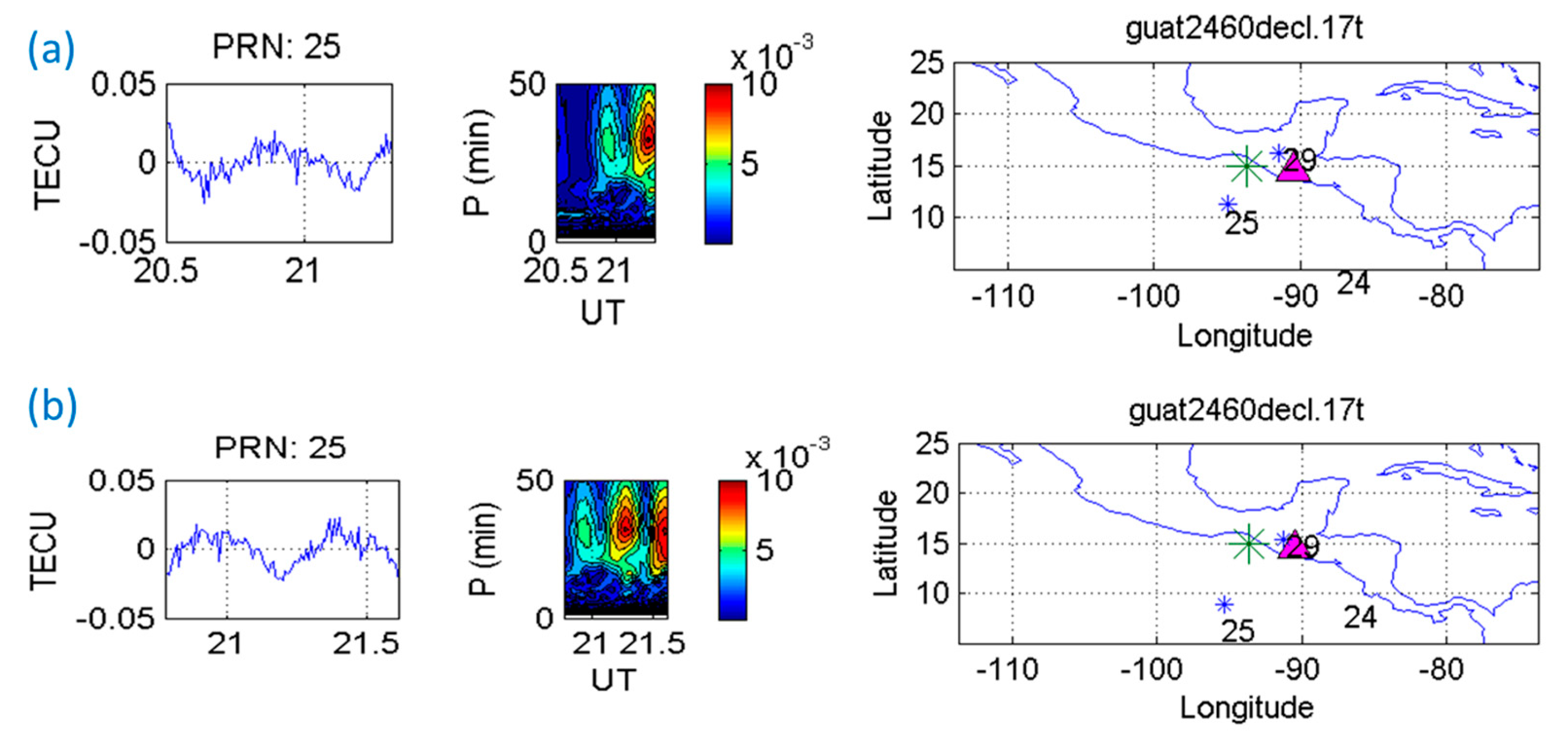
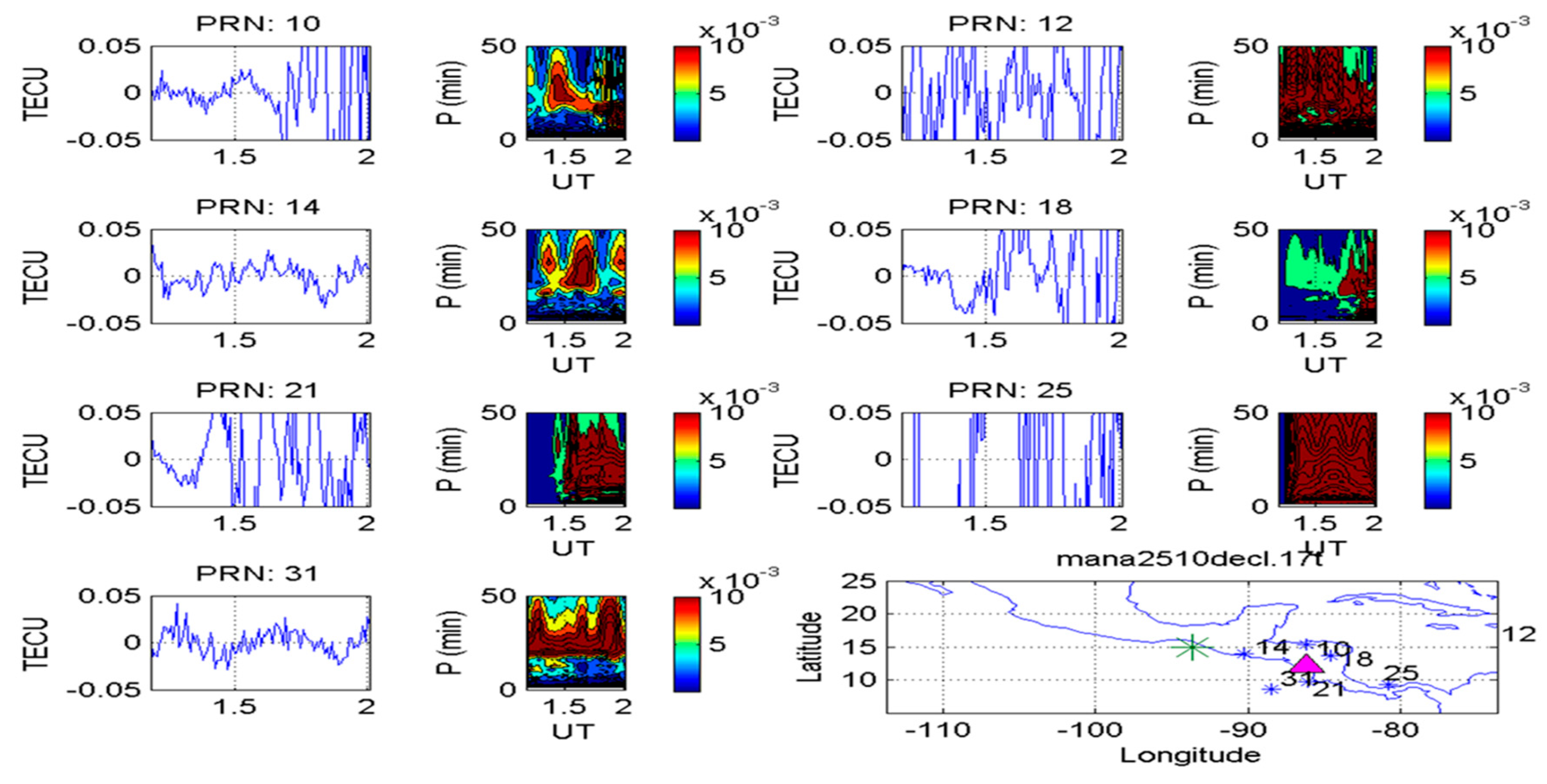
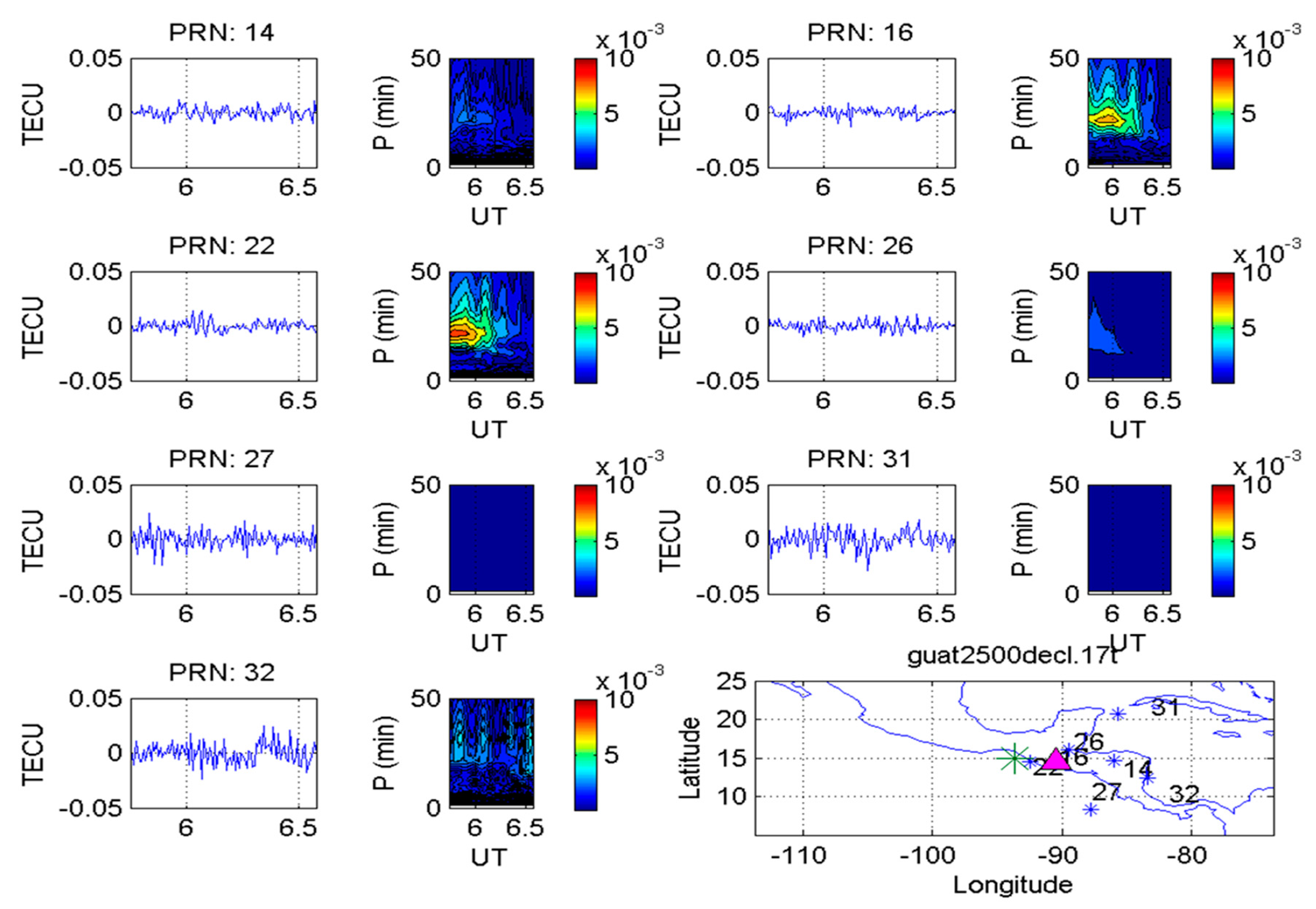
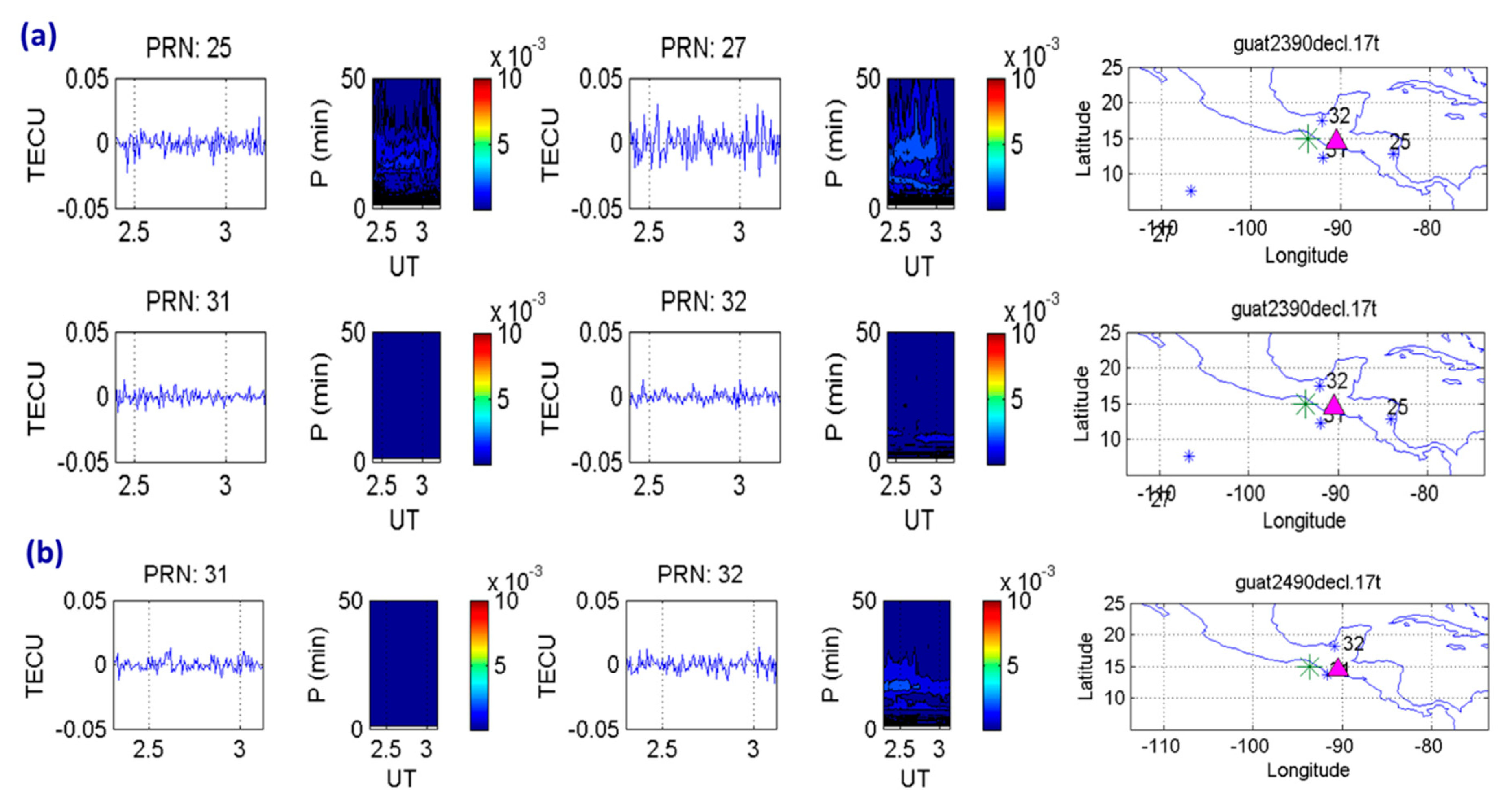
3.1.2. Spectral Analysis of Ionospheric TEC
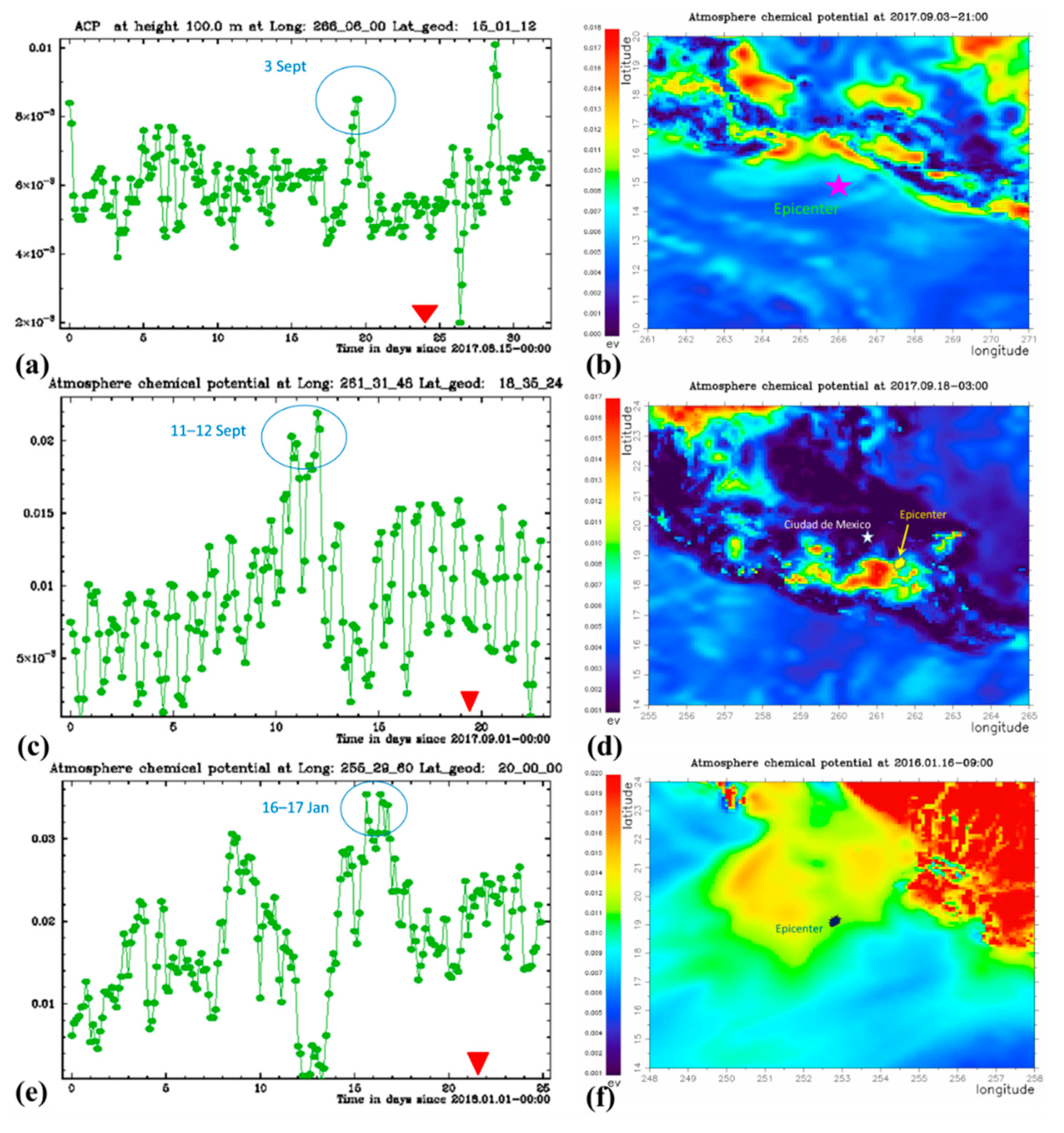
3.2. Atmospheric Analysis
4. Synopsis and Conclusions
Author Contributions
Funding
Institutional Review Board Statement
Informed Consent Statement
Data Availability Statement
Acknowledgments
Conflicts of Interest
References
- Martinelli, G. Contributions to a History of Earthquake Prediction Research. In Pre-Earthquake Processes: A Multidisciplinary Approach to Earthquake Prediction Studies, 5th ed.; John Wiley & Sons: Hoboken, NJ, USA, 2020; pp. 67–76. [Google Scholar] [CrossRef]
- Ouzounov, D.; Pulinets, S.; Liu, J.Y.; Hattori, K.; Han, P. Multiparameter Assessment of Pre-Earthquake Atmospheric Signals. In Pre-Earthquake Processes: A Multidisciplinary Approach to Earthquake Prediction Studies; Ouzounov, D., Pulinets, S., Hattori, K., Taylor, P., Eds.; John Wiley & Sons: Hoboken, NJ, USA, 2018; pp. 339–359. [Google Scholar]
- Ben-Menahem, A.A. A Concise history of Mainstream Seismology: Origins, legacy and perspectives. Bull. Seismol. Soc. Am. 1995, 85, 1202–1225. [Google Scholar]
- Pulinets, S.A.; Boyarchuk, K. Ionospheric Precursors of Earthquakes; Springer: Berlin, Germany, 2004. [Google Scholar]
- Tramutoli, V.; Corrado, R.; Filizzola, C.; Genzano, N.; Lisi, M.; Pergola, N. From visual comparison to robust satellite techniques: 30 years of thermal infrared satellite data analyses for the study of earthquake preparation phases. Boll. Geof. Teor. Appl. 2015, 56, 167–202. [Google Scholar]
- Qiang, Z.J.; Xu, X.D.; Dian, C.G. Thermal infrared anomaly precursor of impending earthquakes. Chin. Sci. Bull. 1991, 36, 319–323. [Google Scholar] [CrossRef]
- Tramutoli, V.; Marchese, F.; Falconieri, A.; Filizzola, C.; Genzano, N.; Hattori, K.; Lisi, M.; Liu, J.-Y.; Ouzounov, D.; Parrot, M.; et al. Tropospheric and Ionospheric Anomalies Induced by Volcanic and Saharan Dust Events as Part of Geosphere Interaction Phenomena. Geosciences 2019, 9, 177. [Google Scholar] [CrossRef]
- Sorokin, V.M.; Chmyrev, V.M.; Hayakawa, M. The formation of ionosphere-magnetosphere ducts over the seismic zone. Planet. Space Sci. 2000, 48, 175–180. [Google Scholar] [CrossRef]
- Namgaladze, A.A.; Klimenko, M.V.; Klimenko, V.V.; Zakharenkova, I.E. Physical mechanism and mathematical modeling of earthquake ionospheric precursors registered in total electron content. Geomagn. Aeron. 2009, 49, 252–262. [Google Scholar] [CrossRef]
- Kuo, C.L.; Huba, J.D.; Joyce, G.; Lee, L.C. Ionosphere plasma bubbles and density variations induced by pre-earthquake rock currents and associated surface charges. J. Geophys. Res. Space Phys. 2011, 116. [Google Scholar] [CrossRef]
- Kuo, C.L.; Lee, L.C.; Huba, J.D. An improved coupling model for the lithosphere–atmosphere–ionosphere system. J. Geophys. Res. Space Phys. 2014, 119, 3189–3205. [Google Scholar] [CrossRef]
- Enomoto, Y. Coupled interaction of earthquake nucleation with deep Earth gases: A possible mechanism for seismo-electromagnetic phenomena. Geophys. J. Int. 2012, 191, 1210–121412. [Google Scholar] [CrossRef]
- Heki, K.; Enomoto, Y. Preseismic ionospheric electron enhancements revisited. J. Geophys. Res. Space Phys. 2013, 118, 6618–6626. [Google Scholar] [CrossRef]
- Namgaladze, A.A. Earthquakes and global electrical circuit. Russ. J. Phys. Chem. B 2013, 7, 589–593. [Google Scholar] [CrossRef]
- Sorokin, V.; Hayakawa, M. Generation of seismic-related DC electric fields and lithosphere–atmosphere—Ionosphere coupling. Mod. Appl. Sci. 2013, 7, 1–25. [Google Scholar] [CrossRef]
- Hegai, V.V.; Kim, V.P.; Liu, J.Y. On a possible seismomagnetic effect in the topside ionosphere. Adv. Space Res. 2015, 56, 1707–1713. [Google Scholar] [CrossRef]
- Pulinets, S.; Ouzounov, D. Lithosphere–atmosphere– ionosphere coupling (LAIC) model—A unified concept for earthquake precursors validation. J. Asian Earth Sci. 2011, 41, 371–382. [Google Scholar] [CrossRef]
- Freund, F. Earthquake forewarning—A multidisciplinary challenge from the ground up to space. Acta Geophys. 2013, 61, 775–807. [Google Scholar] [CrossRef]
- Pulinets, S.; Khachikyan, G. Solar induced earthquakes—Review and new results. In EGU General Assembly 2020, Online, 4–8 May 2020, EGU2020-10821; EGU: Munich, Germany, 2020. [Google Scholar] [CrossRef]
- Pulinets, S.A.; Ouzounov, D.P.; Karelin, A.V.; Davidenko, D.V. Physical bases of the generation of short-term earthquake precursors: A complex model of ionization-induced geophysical processes in the lithosphere-atmosphere-ionosphere-magnetosphere system. Geomagn. Aeron. 2015, 55, 521–538. [Google Scholar] [CrossRef]
- Klimenko, M.V.; Klimenko, V.V.; Zakharenkova, I.E.; Pulinets, S.A.; Zhao, B.; Tzidilina, M.N. Formation mechanism of great positive disturbances prior to Wenchuan earthquake on May 12, 2008. Adv. Space Res. 2011, 48, 488–499. [Google Scholar] [CrossRef]
- Masci, F.; Thomas, J.N.; Secan, J.A. On a reported effect in ionospheric TEC around the time of the 6 April 2009 L’Aquila earthquake. Nat. Hazards Earth Syst. Sci. 2017, 17, 1461–1468. [Google Scholar] [CrossRef]
- Dautermann, T.; Calais, E.; Haase, J.; Garrison, J. Investigation of ionospheric electron content variations before earthquakes in southern California, 2003–2004. J. Geophys. Res. 2007, 112, B02106. [Google Scholar] [CrossRef]
- Zhu, F.; Su, F.; Lin, J. Statistical Analysis of TEC Anomalies Prior to M6.0+ Earthquakes During 2003–2014. Pure Appl. Geophys. 2018, 175, 3441–3450. [Google Scholar] [CrossRef]
- Thomas, J.; Huard, N.J.; Masci, F. A statistical study of global ionospheric map total electron content changes prior to occurrences of M ≥ 6.0 earthquakes during 2000–2014. J. Geophys. Res. Space Phys. 2017, 122, 2151–2161. [Google Scholar] [CrossRef]
- Dobrovolsky, I.; Zubkov, S.; Miachkin, V. Estimation of the size of earthquake preparation zones. Pure Appl. Geophys. 1979, 117, 1025–1044. [Google Scholar] [CrossRef]
- Petraki, E.; Nikolopoulos, D.; Panagiotaras, D.; Cantzos, D.; Yannakopoulos, P.; Nomicos, C.; Stonham, J. Radon-222: A potential short-term earthquake precursor. J. Earth Sci. Clim. Chang. 2015, 6, 282. [Google Scholar] [CrossRef]
- Ghosh, D.; Deb, A.; Sengupta, R. Anomalous radon emission as precursor of earthquake. J. Appl. Geophys. 2009, 69, 67–81. [Google Scholar] [CrossRef]
- Riggio, A.; Santulin, M. Earthquake forecasting: A review of radon as seismic precursor. Boll. Geofis. Teor. Appl. 2015, 56, 95–114. [Google Scholar]
- Paudel, S.R.; Banjara, S.P.; Wagle, A.; Freund, F.T. Earthquake chemical precursors in groundwater: A review. J. Seismol. 2018, 22, 1293–1314. [Google Scholar] [CrossRef]
- Grammakov, A.G. On the influence of some factors in the spreading of radioactive emanations under natural conditions. Zhur. Geofiz. 1936, 6, 123–148. [Google Scholar]
- Clements, W.E. The Effect of Atmospheric Pressure Variation on the Transport of 222Rn from the Soil to the Atmosphere. Ph.D. Thesis, New Mexico Institute of Mining and Technology, Sorocco, NM, USA, 1974. [Google Scholar]
- Roffman, A. Short-Lived Daughter Ions of Radon 222 in Relation to Some Atmospheric Processes. J. Geophys. Res. 1972, 77, 5883–5899. [Google Scholar] [CrossRef]
- Boyarchuk, K.A.; Karelin, A.V.; Shirokov, R.V. Bazovaya Model’ Kinetiki Ionizirovannoi Atmosfery (The Reference Model of Ionized Atmospheric Kinetics); VNIIEM: Moscow, Russia, 2006. [Google Scholar]
- Harrison, R.G.; Aplin, K.L.; Rycroft, M.J. Atmospheric electricity coupling between earthquake regions and the ionosphere. J. Atmos. Sol. Terr. Phys. 2010, 72, 376–381. [Google Scholar] [CrossRef]
- Silva, H.G.; Bezzeghoud, M.; Reis, A.H.; Rosa, R.N.; Tlemçani, M.; Araújo, A.A.; Serrano, C.; Borges, J.F.; Caldeira, B.; Biagi, P.F. Atmospheric electrical field decrease during the M = 4.1 Sousel earthquake (Portugal). Nat. Hazards Earth Syst. Sci. 2011, 11, 987–991. [Google Scholar] [CrossRef]
- Willet, J. Atmospheric-electric implications of 222Rn daughter deposition on vegetated ground. J. Geophys. Res. 1985, D90, 5901–5908. [Google Scholar] [CrossRef]
- Holzer, R.E. Atmospheric Electrical Effects of Nuclear Explosions. J. Geophys. Res. 1972, 77, 5845–5855. [Google Scholar] [CrossRef]
- Silva, H.G.; Oliveira, M.M.; Serrano, C.; Bezzeghoud, M.; Reis, A.H.; Rosa, R.N.; Biagi, P.F. Influence of seismic activity on the atmospheric electric field in Lisbon (Portugal) from 1955 to 1991. Ann. Geophys. 2012, 55, 193–197. [Google Scholar]
- Rulenko, O.P. Operative precursors of earthquakes in the near-ground atmosphere electricity. Volcanol. Seismol. 2000, 4, 57–68. [Google Scholar]
- Ciraolo, L. Evaluation of GPS L2-L1 biases and related daily TEC profiles. In Proceedings of the GPS/Ionosphere Workshop; DLR/DFD, Dtsch. Forsch. fuer Luft und Raumfahrt./Dtsch. Fehrnerkundsdatezentrum: Neustrelitz, Germany, 1993; pp. 90–97. [Google Scholar]
- Klotz, S.; Johnson, N.L. Encyclopedia of Statistical Sciences; Wiley: Hoboken, NJ, USA, 1983. [Google Scholar]
- Hocke, K.; Schlegel, K. A review of atmospheric gravity waves and travelling ionospheric disturbances: 1982–1995. Ann. Geophys. 1996, 14, 917–940. [Google Scholar] [CrossRef]
- Pulinets, S.A.; Boyarchuk, K.A.; Lomonosov, A.M.; Khegai, V.V.; Liu, J.Y. Ionospheric Precursors to Earthquakes: A Preliminary Analysis of the foF2 Critical Frequencies at Chung-Li Ground-Based Station for Vertical Sounding of the Ionosphere (Taiwan Island). Geomagn. Aeron. 2002, 42, 508–513. [Google Scholar]
- Pulinets, S.; Ouzounov, D.; Karelin, A.; Dmitry Davidenko, D. Lithosphere–atmosphere–ionosphere–magnetosphere coupling—a concept for pre-earthquake signals generation. In Pre-Earthquake Processes: A Multidisciplinary Approach to Earthquake Prediction Studies; John Wiley & Sons: Hoboken, NJ, USA, 2018; pp. 79–99. [Google Scholar] [CrossRef]
- Muslim, B.; Efendi, J.; Suryanal, D.R. Developing near real time TEC computation system from GPS data for improving spatial resolution of ionospheric observation over Indonesia. In Proceedings of the 1st International Seminar on Space-Science and Technology, Serpong, Indonesia, 3 December 2013. [Google Scholar]
- Gao, Y.; Liu, Z.Z. Precise ionosphere modeling using regional GPS network data. Positioning 2002, 1, 24–28. [Google Scholar] [CrossRef]
- Pulinets, S.A.; Ouzounov, D.; Karelin, A.V.; Boyarchuk, K.A.; Pokhmelnykh, L.A. The physical nature of the thermal anomalies observed before strong earthquakes. Phys. Chem. Earth Parts A/B/C 2006, 31, 143–153. [Google Scholar] [CrossRef]
- Marchetti, D.; Akhoondzadeh, M. Analysis of Swarm satellites data showing seismo-ionospheric anomalies around the time of the strong Mexico (Mw=8.2) earthquake of 08 September (2017). Adv. Space Res. 2018, 62, 614–623. [Google Scholar] [CrossRef]
- Sergeeva, M.A.; Maltseva, O.A.; Gonzalez-Esparza, J.A.; Mejia-Ambriz, J.C.; De la Luz, V.; Corona-Romero, P.; Gonzalez, L.X.; Gatica-Acevedo, V.J.; Romero-Hernandez, E.; Rodriguez-Martinez, M.; et al. TEC behavior over the Mexican region. Ann. Geophys. 2018, 61, 104. [Google Scholar] [CrossRef]
- Astafyeva, E.; Heki, K. Vertical TEC over seismically active region during low solar activity. J. Atmos. Sol. Terr. Phy. 2011, 73, 1643–1652. [Google Scholar] [CrossRef]
- Afraimovich, E.L.; Astafyeva, E.I. TEC anomalies—Local TEC changes prior to earthquakes or TEC response to solar and geomagnetic activity changes? Earth Planets Space 2008, 60, 961–966. [Google Scholar] [CrossRef]
- Afraimovich, E.L.; Astafyeva, E.I.; Oinats, A.V.; Yasukevich, Y.V.; Zhivetiev, I.V. Global electron content: A new conception to track solar activity. Ann. Geophys. 2008, 26, 335–344. [Google Scholar] [CrossRef]
- Sotomayor-Beltran, C. Ionospheric anomalies preceding the low- latitude earthquake that occurred on April 16, 2016 in Ecuador. J. Atmos. Sol. Terr. Phys. 2019, 182, 61–66. [Google Scholar] [CrossRef]
- Duma, G.; Freund, F.F. Undoubtedly, solar flare activity acts as a trigger for strong earthquakes. In Geophysical Research Abstracts; EGU: Munich, Germany, 2019; Volume 21. [Google Scholar]
- Jin, S.; Jin, R.; Liu, X. GNSS Atmospheric Seismology: Theory, Observations and Modeling; Springer: Berlin/Heidelberg, Germany, 2019. [Google Scholar]
- Sharma, G.; Mohanty, S.; Kannaujiya, S. Ionospheric TEC modelling for earthquakes precursors from GNSS data. Quat. Int. 2017, 462, 65–74. [Google Scholar] [CrossRef]
- Pulinets, S.A.; Legen’ka, A.D. Dynamics of the near-equatorial ionosphere prior to strong earthquakes. Geomagn. Aeron. 2002, 42, 239–244. [Google Scholar]
- Pulinets, S. Low-latitude atmosphere-ionosphere effects initiated by strong earthquakes preparation process. Int. J. Geophys. 2012, 2012. [Google Scholar] [CrossRef]
- Ryu, K.; Lee, E.; Chae, J.; Parrot, M.; Pulinets, S. Seismo-ionospheric coupling appearing as equatorial electron density enhancements observed via DEMETER electron density measurements. J. Geophys. Res. Space Phys. 2014, 119, 8524–8542. [Google Scholar] [CrossRef]
- Oikonomou, C.; Haralambous, H.; Muslim, B. Investigation of ionospheric precursors related to deep and intermediate earthquakes based on spectral and statistical analysis. Adv. Space Res. 2017, 59, 587–602. [Google Scholar] [CrossRef]
- Sun, Y.Y.; Liu, J.Y.; Wu, T.Y.; Chen, C.H. Global Distribution of Persistence of Total Electron Content Anomaly. Atmosphere 2019, 10, 297. [Google Scholar] [CrossRef]
- Pulinets, S. Physical mechanism of the vertical electric field generation over active tectonic faults. Adv. Space Res. 2009, 44, 767–773. [Google Scholar] [CrossRef]
- Nenovski, P.I.; Pezzopane, M.; Ciraolo, L.; Vellante, M.; Villante, U.; De Lauretis, M. Local changes in the total electron content immediately before the 2009 Abruzzo earthquake. Adv. Space Res. 2015, 55, 243–258. [Google Scholar] [CrossRef][Green Version]
- Somsikov, V.M. Atmospheric Waves Caused by the Solar Terminator: A Review. Geomagn. Aeron. 1991, 31, 1–12. [Google Scholar]
- Afraimovich, E.L.; Edemskiy, I.K.; Voeykov, S.V.; Yasyukevich, Y.V.; Zhivetiev, I.V. The first GPS-TEC imaging of the space structure of MS wave packets excited by the solar terminator. Ann. Geophys. 2009, 27, 1521–1525. [Google Scholar] [CrossRef]
- Pulinets, S.; Davidenko, D. Ionospheric precursors of earthquakes and global electric circuit. Adv. Space Res. 2014, 53, 709–723. [Google Scholar] [CrossRef]
- Dunajecka, M.A.; Pulinets, S.A. Atmospheric and thermal anomalies observed around the time of strong earthquakes in Mexico. Atmósfera 2005, 18, 235–247. [Google Scholar]
- Pulinets, S.; Ouzounov, D.; Davydenko, D.; Petrukhin, A. Multiparameter monitoring of short-term earthquake precursors and its physical basis. Implementation in the Kamchatka region. In E3S Web of Conferences; EDP Sciences: Ulis, France, 2016; Volume 11, p. 00019. [Google Scholar]
- Pulinets, S.A.; Morozova, L.I.; Yudin, I.A. Synchronization of atmospheric indicators at the last stage of earthquake preparation cycle. Res. Geophys. 2014. [Google Scholar] [CrossRef]
- Ouzounov, D.; Liu, D.; Chunli, K.; Cervone, G.; Kafatos, M.; Taylor, P. Outgoing long wave radiation variability from IR satellite data prior to major earthquakes. Tectonophysics 2007, 431, 211–220. [Google Scholar] [CrossRef]
- Parrot, M.; Tramutoli, V.; Liu, T.J.; Pulinets, S.; Ouzounov, D.; Genzano, N.; Lisi, M.; Hattori, K.; Namgaladze, A. Atmospheric and ionospheric coupling phenomena related to large earthquakes. Nat. Hazards Earth Syst. Sci. 2016. [Google Scholar] [CrossRef]


| Seismic Events No | Date | TIME Hour (UT) | Magnitude (R) | Preparation Area Radius (km) | Depth (km) | Latitude (°) | Longitude (°) | Epicenter Region |
|---|---|---|---|---|---|---|---|---|
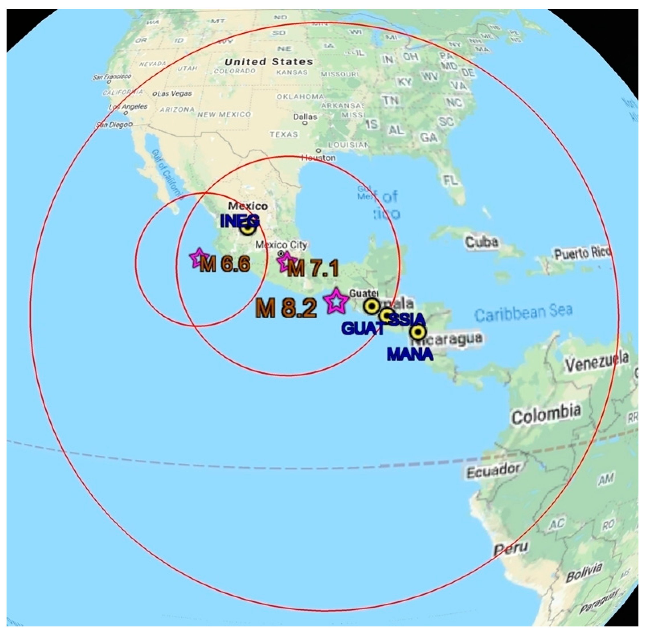
| 1 | 8-September-2017 | 4:49:19 | 8.2 | 3357 | 47.39 | 15.02 | −93.90 | 101 km SSW of Tres Picos, Mexico |
| 2 | 19-September-2017 | 18:14:38 | 7.1 | 1130 | 48 | 18.55 | 98.49 | Ayutla, Mexico |
| 3 | 21-January-2016 | 18:06:57 | 6.6 | 689 | 10 | 18.82 | 106.93 | Tomatlan, Mexico |
| A | B | C | D | |
|---|---|---|---|---|
| Earthquakes Having Ionospheric TEC Anomalies | Earthquakes Prior to Which Positive ‘Mexico’ TEC Anomalies Occur | Earthquakes Prior to Which TEC Anomalies Occur Due to Geomagnetic Conditions | Earthquakes Having TEC Anomalies Happening Close to Geomagnetic Storms | |
| Positive TEC | Negative TEC | |||
| 8.2 Mw, September 8 | 4.6 Mw, January 15 | 4.8 Mw, June 5, due to EQ or ‘Mexico’ positive TEC anomaly | 5 Mw, January 4 unsettled conditions | 5.3 Mw, May 26 |
| 4.6 Mw, March 21 | 5.5 Mw, June 10 ‘Mexico’ positive TEC anomaly | 4.9 Mw, January 9 unsettled conditions | 5.1 Mw, 4.6 Mw, July 5, also due to EQ | |
| 5.0 Mw, June 13 | 4.7 Mw, August 27 ‘Mexico’ positive TEC anomaly or close to geom. storm | 5.3 Mw, January 12 unsettled conditions | 4.7 Mw, August 27 | |
| 4.8 Mw, June 5, due to EQ or ‘Mexico’ positive TEC anomaly | 6.9 Mw, June 14 | 5.0 Mw, August 31 ‘Mexico’ positive TEC anomaly or close to geom. storm | 4.6 Mw, March 10 recovery phase | 5.0 Mw, August 31 |
| 5.5 Mw, June 10, due to EQ or ‘Mexico’ positive TEC anomaly | 4.8 Mw, March 12 recovery phase | 8.2 Mw, September 8, also storm main phase | ||
| 5.0 Mw, August 31, due to EQ, ‘Mexico’ positive TEC anomaly | 4.4 Mw, Febuary 28, only ‘Mexico’ positive TEC anomaly | 4.7 Mw, March 13 recovery phase | 4.3 Mw, October 30, also unsettled (1 anomaly inside and 1 close storm conditions) | |
| 4.6 Mw, October 12, only ‘Mexico’ positive TEC anomaly | 5.3 Mw, May 30 recovery phase | 5.1 Mw, December 15 | ||
| 5.1 Mw, 4.6 Mw, July 5 or close to geom. storm | 5.2 Mw, November 4, only ‘Mexico’ positive TEC anomaly | 5.4 Mw, May 31 recovery phase | 5.3 Mw, December 29 | |
| 6.8 Mw, June 22 unsettled conditions | ||||
| 4.3 Mw, June 26 unsettled conditions | ||||
| 4.4 Mw, July 10 recovery phase | ||||
| 4.8 Mw, July 19 recovery phase | ||||
| 5.1 Mw, July 5, unsettled conditions but also due to earthquake | ||||
| 4.6 Mw, July 5, unsettled conditions but also due to earthquake | ||||
| 5.3 Mw, August 20, unsettled conditions | ||||
| 5.3 Mw, August 21, unsettled conditions | ||||
| 8.2 Mw, September 8, storm main phase | ||||
| 7.1 Mw, September 19, recovery phase | ||||
| 4.9 Mw, September 20, recovery phase | ||||
| 4.6 Mw, October 12, inside 2 consecutive storms | ||||
| 4.3 Mw, October 30, unsettled (1 anomaly inside and 1 close to geom. storm conditions) | ||||
| 4.3 Mw, November 20, Earthquake happened 1 day before geom. storm | ||||
| 4.3 Mw, November 8, Earthquake happened start of recovery phase | ||||
| 6.5 Mw November 13 recovery phase | ||||
| 5.1 Mw December (1 anomaly inside and 1 close storm conditions) | ||||
| 5.3 Mw December (1 anomaly inside and 1 close storm conditions) | ||||
Publisher’s Note: MDPI stays neutral with regard to jurisdictional claims in published maps and institutional affiliations. |
© 2020 by the authors. Licensee MDPI, Basel, Switzerland. This article is an open access article distributed under the terms and conditions of the Creative Commons Attribution (CC BY) license (http://creativecommons.org/licenses/by/4.0/).
Share and Cite
Oikonomou, C.; Haralambous, H.; Pulinets, S.; Khadka, A.; Paudel, S.R.; Barta, V.; Muslim, B.; Kourtidis, K.; Karagioras, A.; İnyurt, S. Investigation of Pre-Earthquake Ionospheric and Atmospheric Disturbances for Three Large Earthquakes in Mexico. Geosciences 2021, 11, 16. https://doi.org/10.3390/geosciences11010016
Oikonomou C, Haralambous H, Pulinets S, Khadka A, Paudel SR, Barta V, Muslim B, Kourtidis K, Karagioras A, İnyurt S. Investigation of Pre-Earthquake Ionospheric and Atmospheric Disturbances for Three Large Earthquakes in Mexico. Geosciences. 2021; 11(1):16. https://doi.org/10.3390/geosciences11010016
Chicago/Turabian StyleOikonomou, Christina, Haris Haralambous, Sergey Pulinets, Aakriti Khadka, Shukra R. Paudel, Veronika Barta, Buldan Muslim, Konstantinos Kourtidis, Athanasios Karagioras, and Samed İnyurt. 2021. "Investigation of Pre-Earthquake Ionospheric and Atmospheric Disturbances for Three Large Earthquakes in Mexico" Geosciences 11, no. 1: 16. https://doi.org/10.3390/geosciences11010016
APA StyleOikonomou, C., Haralambous, H., Pulinets, S., Khadka, A., Paudel, S. R., Barta, V., Muslim, B., Kourtidis, K., Karagioras, A., & İnyurt, S. (2021). Investigation of Pre-Earthquake Ionospheric and Atmospheric Disturbances for Three Large Earthquakes in Mexico. Geosciences, 11(1), 16. https://doi.org/10.3390/geosciences11010016