1. Introduction
The development of geomathematics in the past was a very dynamic and non-linear process. In the early days (until the 1980s) geomathematics and geostatistics were considered as synonymous, so pioneer works in geostatistics were considered as breakthroughs in the entire geomathematics applied in geosciences. The first results of geostatistical research (different from research in the field of “spatial statistics”) had been published by [
1,
2,
3] where kriging was described for the first time. The same algorithm had already been applied earlier by [
4] for estimation of gold nuggets concentrations in South African mines. Matheron’s foundation has been based on the least square method and linear Gaussian model, which stayed as a base until the present day. Following the linear models, authors such as [
5] and [
6] also developed non-parametric and non-linear geostatistics. In parallel, geostatistics was developed together with applied statistics by [
7]. Cressie [
8] made an important step toward unification of geostatistics and other data analysis methods in geology, describing three main branches of spatial statistics-geostatistics, spatial variations and spatial point processes. That is what we today call geomathematics.
Here it is also worth mentioning some pioneer works that preceded Matheron’s development of early geostatistics. Frits Agterberg published some early papers crucial for later development of spatial statistics. He used numerical analysis of depositional and structural data to interpret sedimentation rates [
9] as well as divergent structural trends [
10] and single structural events. In Agterberg [
11] the origin of skewed distributions of ore minerals was discussed and spatial dependence recognized using Fourier analysis. Krumbein [
12,
13,
14] developed and published several statistical models in geological mapping. Approximating simulations with Matheron works, Vistelius [
15] published important studies in mathematical geology, and Merriam [
16] undertook the early application of computers in geology.
Here, it is important to mention that the use of geostatistics (even statistics) is closely related with exploration and the production of hydrocarbon reservoirs (e.g., [
17,
18]). In the late 1980s, geostatistics offered new algorithms, allowing much better reservoir characterisation to be obtained, in particular visualisation. However, from the early days in geostatistics and later geomathematics, the main factor in the selection of a method was the number and distribution of data elements. Those two problems are often intertwined, although distribution of data is considered as fundamental for any later analysis.
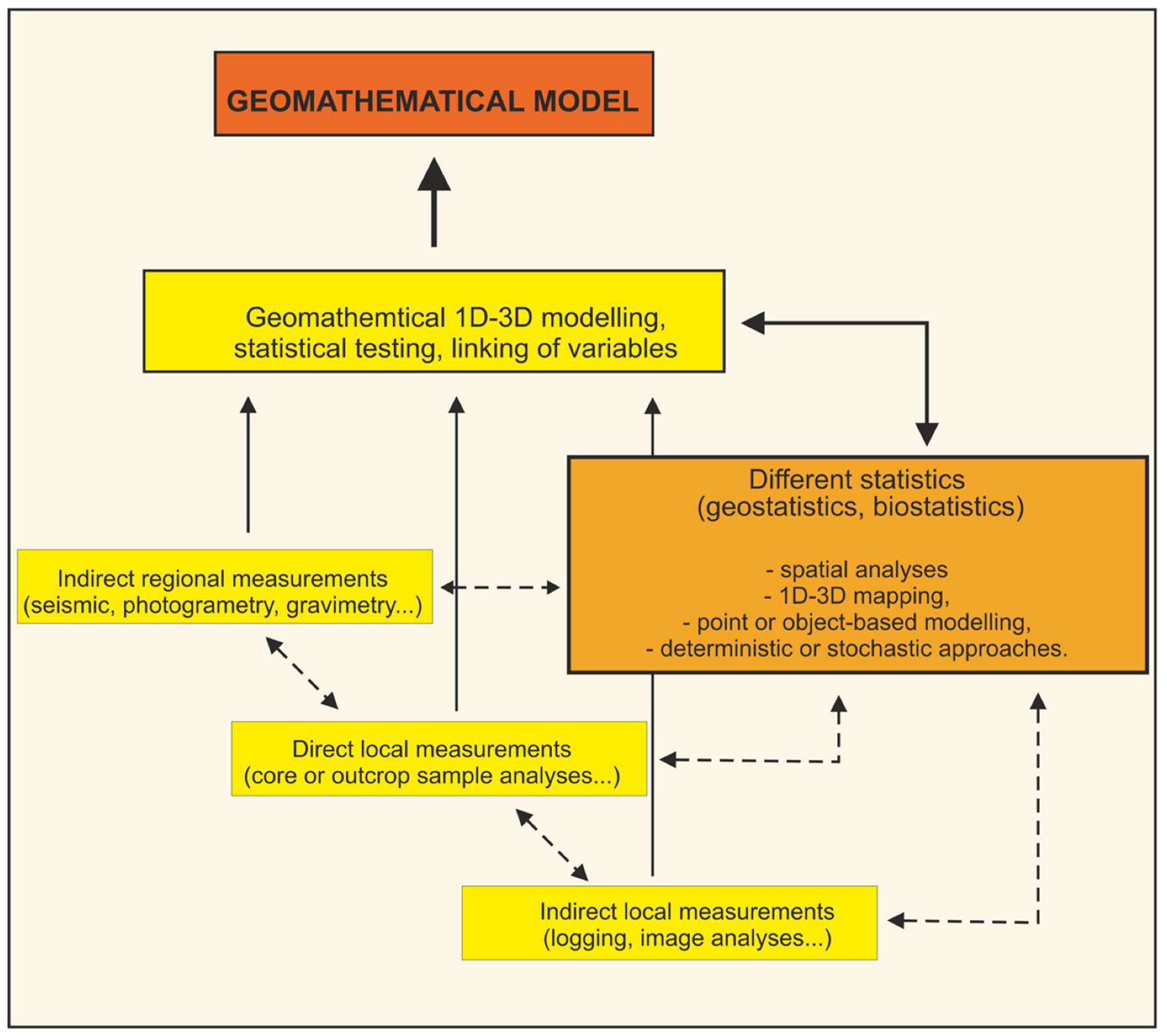
As in any data-based analysis, geomathematics is highly dependent on hard data, i.e., measurements, aiming to predict values in non-sampled volumes (
Figure 1). The problem had been solved differently. As geological variables are mostly presented in deterministic ways, knowledge about (sub)surface is always partial. In fact, the models are stochastic but too complex so that available mathematical approximations, restricted with limited data, could be presented in such a way. Geomathematics offered the approaches designed for object-based models, where objects are datasets analysed and visualised with different spatial methods (e.g., [
19,
20]). Most of them are deterministic (kriging) but some approaches could be stochastic (simulations).
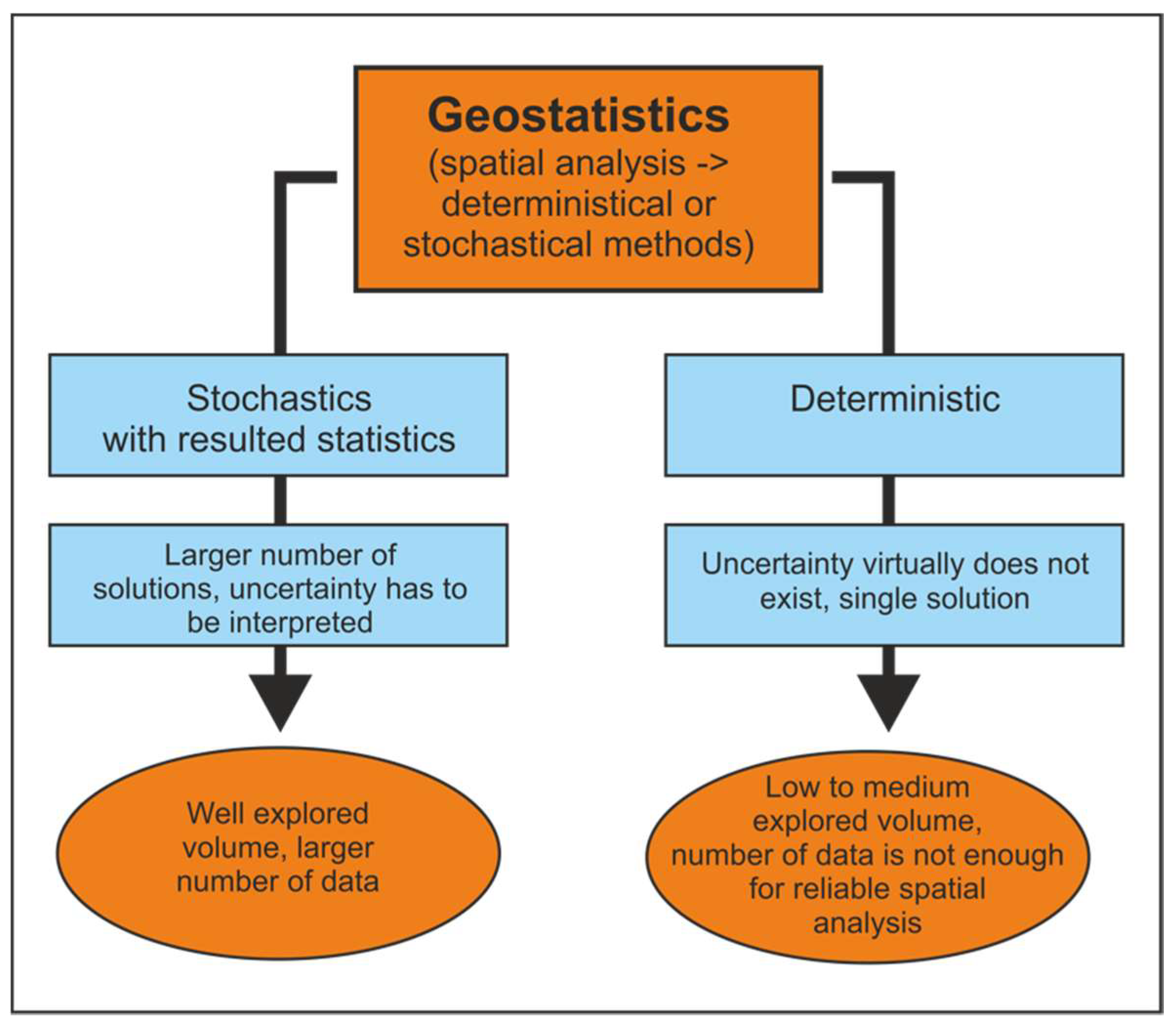
Any classification of such models can be categorised. Here we decided to divide them into:
Full deterministic, models where volume is well known, without uncertainties, possible correlated, and settings are known and established. Such knowledge is rare, but many areas are approximated in such a way.
Stochastic volumes, where uncertainties cannot be full described and permanently exists. However, the probability model allows predictions and estimations to be made with different geomathematical algorithms. This is mostly done with analysed (sub)surface volumes, but the stochastic approach asks for more experiences and, contradictorily, more data than the deterministic approach.
Unpredictable volumes, where analysed variables could not be described by any algorithm or just the number of data elements is not high enough so that any observation is valid and general.
The key goal for any geomathematical analysis is the definition of a typical model that can be applied for further prognosis in similar or the same conditions. Any such prognosis needs to be based on valid choices, grounded on previous case studies where decision trees are made. Such choices are always based on the number of inputs, regarding variables and dataset size. Generally, the explored geological volume is researched longer so that the object of researching could be improved more easily with both deterministic or stochastic approaches. The decision depends on experience, knowledge and readiness to accept uncertainties in future estimations. Any multivariable approach is beneficial (like co-kriging) but needs well-documented connections among dependent variables. Significant inherited (measurements limitations, equipment error) and man-made (biased sampling) uncertainties forced stochastics, but limitation of such an approach is a must-have spatial model. However, it is not a condition at all for simpler algorithms like inverse distance weighting (IDW), the modified Shepard’s method (MSM), nearest neighbourhood (NN) or similar. The largest limitation is the number of data elements (
Figure 2), especially if the primary variable is to be defined in the entire dataset. The sparse or non-representative dataset greatly limits the application of statistics. Even statistical representative sets (e.g., n > 30) are much easier when analysed with parametric statistics that require Gaussian distribution. By contrast, non-parametric statistics are only a choice, which can limit the number of tests and mapping, in particular.
However, and despite all limitations, geomathematics has many favourable and robust tools and algorithms for analysis of almost all geological datasets. It is especially valid if geomathematics is considered as a field divided into three sub-fields: geostatistics, statistics applied to geosciences and neural networks applied to geoscientific data.
The main challenge is the selection of an appropriate procedure. How to find such tools, but only in a very tiny spectre of geomathematics and geosciences, has been presented in this work, through the examples of two different geomathematical subfield datasets. The first one refers to the subsurface geological mapping, as described above, and the second one refers to palaeontology and biostatistics.
The starting point in paleontological research is the assumption presented by day biota and processes which are the key to understanding Earth’s history. Therefore, the biological research methods and facts, such as biostatistics (biological statistics or biometry), are common in taxonomical and palaeoecological studies in palaeontology due to the assumption that species can be defined by morphology, including the measurable parameters.
The development of biostatistics dates back to the 19th century, with Francis Galton (1822−1911), “the father of biostatistics and eugenics”. His methodology, used in the analysis of biological variation, is considered as the foundation for the application of statistics to biology [
13]. The term “biometry” was coined by the zoologist W.F.R. Wilson (1860−1906), who was working with Karl Pearson on the application of statistical methods in biology [
21]. The application of biometry in the systematic description of plants and animals was pointed out by [
22], where he describes the necessity of specific descriptions of taxon characteristics, in order to precisely describe the specimen. The rising impact of biometry resulted in the establishment of the Biometric Society on 6 September 1947 at Woods Hole, USA, as described by [
23]. The first president of the Biometric Society was Sir Ronald Aylmer Fisher (1890−1962). The society was later renamed the International Biometric Society. The Biometric Section of the American Statistical Association started publishing the Biometrics Bulletin in 1945, which was renamed Biometrics in 1947.
Two significantly different datasets and applications in geological subsurface mapping and biostatistics (biometrics) presented in this paper, represent, in the last decade, as well as currently, the most progressive and publicised geomathematical subfields in Croatian geology.
2. Mathematical Basics of Algorithms Applied in the Presented Case Studies
2.1. Kriging Method
Kriging (as well as the co-kriging and stochastic simulations) is a group of statistical estimation methods. The specificity of kriging (e.g., [
5,
24,
25]) is the definition as the best linear unbiased estimator (BLUE), although it is valid only for specific datasets. The strength of the kriging approach is due to the weighting coefficient calculation, the procedure based on the minimisation of kriging variance. The linear method means that estimation has been done by the combination of hard data; the unbiased character makes sure that the estimation’s expected value is as real as for the entire possible population. The estimator defines the applied methodology. The linear estimation is shown in Equation (1):
where:
- Zk
value of the regionalised variable (variable that described some geological property in a selected space with clear structure and known statistics) calculated at location “k”;
- Zi
value of the regionalised variable measured at location “I”;
- λi
weighting coefficient calculated by kriging matrices for location “I”.
The necessary condition for the kriging estimation is that the measured Zi values are characterised with normal distribution or, at least, that such property is assumed for that variable in the case of a large number of measurements. Compared with simpler estimation algorithms, kriging is a more time-consuming interpolation method, but also better tool for handling with highly clustered data. By contrast, the kriging results in very weak works with small datasets (n < 20), unable to give an origin to meaningful spatial models. The spatial (variogram, co-variance or madogram) tools are powerful when applied with enough data and background knowledge. The variogram is the most often applied among them. It is defined as squared difference between two pints at some distance.
As mentioned earlier, the main advantage of kriging is the weighting coefficient calculation. After the spatial model has been set up, the calculation of the coefficient is not dependent on their value, but exclusively on the distance between measured points and location where the value is not known. Such a value is also called “statistical distance” or “semivariogram distance”, referring to their derivation from the variogram (value of variance for any data-pair, which is function of their distance; once variogram model is calculated, the variogram for new measurements can be calculated only from the distance itself, regardless of their value). The kriging equations (Equation (2)) are calculated using matrices. In two of them (W, B), the values are given with variogram values, which depend on distances among observed locations:
There are numerous kriging techniques, each of them differenced by some modification in matrices. The most used in Croatian case studies are herein designated by simple, ordinary, indicator and universal kriging. Simple kriging is the basis for all the other available techniques. The matrix is presented in Equation (3):
where γ—variogram value, Z
1…Z
n—known measured values in spatial points (hard data), x—location where value is estimated from known values, λ—weighed coefficients for location 1…n.
Although the basic technique, it is the only one that do not satisfy the condition of unbiased estimation, because it is the only equation without constraint. Such constraint(s) could be linear or non-linear.
The technique used most often is presented in Equation (4) with an additional constraint, the Lagrange multiplier (μ), aiming to find the local minima and maxima of the function, subjected to equality constraints, i.e., to minimise the kriging variance.
2.2. Inverse Distance Weighting (IDW) Interpolation Method
IDW is a widely used interpolation method, both for small and large datasets. The unknown value is calculated based on all known points and inversely proportional to their distances, weighted by power exponent (Equation (5), e.g., [
26,
27,
28]) and is defined as:
where:
- ZIU
estimated value,
- d1…dn
distance between locations (points) with measurements (1…n) and estimated location (IU),
- p
power (distance) exponent,
- z1…zn
known values at locations 1…n.
The mapping results are greatly influenced by the power exponent, which could stress the influence of more distance points and smooth the map (for
p <= 2) or force very local estimation (
p > 2) and even, for large “
p”, result in zonal estimation, i.e., in map like Voronoi polygons. This method has been proved for mapping problems in the Croatian part of the Pannonian Basin System (CPBS) for all datasets where clustering was not largely imposed, and for datasets smaller than 15 points too (e.g., [
29,
30]).
2.3. Basics of the Nearest Neighbourhood (NN) Estimation Method
NN is the simplest statistical estimation method when an unknown point is estimated only from the closest known value. The results are valued polygons, like the Voronoi diagram. The distance between the points is Euclidean (Equation (6)):
where:
- d
distance,
- n
n-th pair of points,
- x and T
unknown and measured point,
- X and T
length of line segment in Euclidean space connecting the points X and T for pairs 1…n, in the Euclidian n-space.
The method is meaningful to apply only for very small datasets, like 5 or fewer points. The output is not a map, but a schematic polygon view.
2.4. Basics of the Natural Neighbourhood (NaN) Estimation Method
NaN is the modification of the NN and results are also shown as Voronoi diagrams (polygons). The unknown point is estimated from several nearest points (e.g., [
31,
32,
33]) using Equation (7):
where:
- X(x,y)
estimated value in point (x,y),
- A(Xi,Yi)
known value in point (Xi,Yi),
- wi
proportion of polygon, i“ in total area.
2.5. Modified Shepard’s Method (MSM)
The MSM interpolation is a modification of the IDW method, with the aim of reducing the expressive local values (outliers, extremes) that could cause “bull’s-eyeing” or “butterfly shape” effects. The method was developed by [
34] and it is why is named as Shepard’s method. The modification of the method was carried out in the works of, e.g., [
35,
36]. The estimation is done by Equation (8):
where:
- F
MSM function,
- W
relative weights,
- Qk
bivariate quadratic function,
- x, y
data coordinates,
- n
number of data elements.
MSM used so called relative weights determined (Equation (9)):
where:
- dk
Euclidean distance between points at locations (x, y) and (xk, yk),
- Rω
radius of influence around node (xk, yk).
2.6. Cross-Validation as Numerical Estimation of Mapping Error
Cross-validation is a numerical procedure which can be applied also as error-based comparison tool for several maps with the same input, but sequentially interpolated with two or more methods. The procedure is repeated as many times as there are measured (hard) values, dropping one known point out and calculating the estimation in the same location from the rest of the hard data (Equation (10)). One of the measures that can be calculated based on cross-validation are mean square error (MSE, e.g., [
29,
37,
38,
39]). This value is often used as criteria for the most appropriate map selection in the case of small datasets in the CPBS (e.g., [
40,
41]).
where:
- MSE
mean square error value,
- n
number of known values,
- SV
measured value in point “i”,
- P
estimated value in point “i”,
- i
i-th point.
2.7. Shannon–Wiener Index or Shannon Diversity Index (H)
In paleoecological analyses, one of the goals is to explore species richness and diversity in the analysed data sets, and to compare biological diversity between the samples with an uneven number of species and individuals. In the examples presented in this paper (e.g., see here Figure 6), authors showed part of the research on the biodiversity of microfossils Foraminifera, where the Shannon–Wiener or Shannon diversity index (H) (called also Shannon entropy in informatics) is used as one of the measures of species diversity in one sample, and between samples [
34]. The “H” is calculated by Equation (11) [
42]:
where:
- pi
a proportion of individuals belonging to the ith species in the sample,
- ln
a natural logarithm,
- R
total number of species in the community (richness).
Equation (11) shows dependence of H (Shannon index) on p
i (proportion of individuals, and if all species in the sample are equally represented, H is at its maximum [
42].
3. Recent Advances in Geomathematical Mapping in Small Datasets and Case Studies from Croatia
During 2019 and 2020, broad testing of small datasets mapping has been applied [
41,
43] to the CPBS. A small subsurface sample set is considered to be a set of measurements which includes [
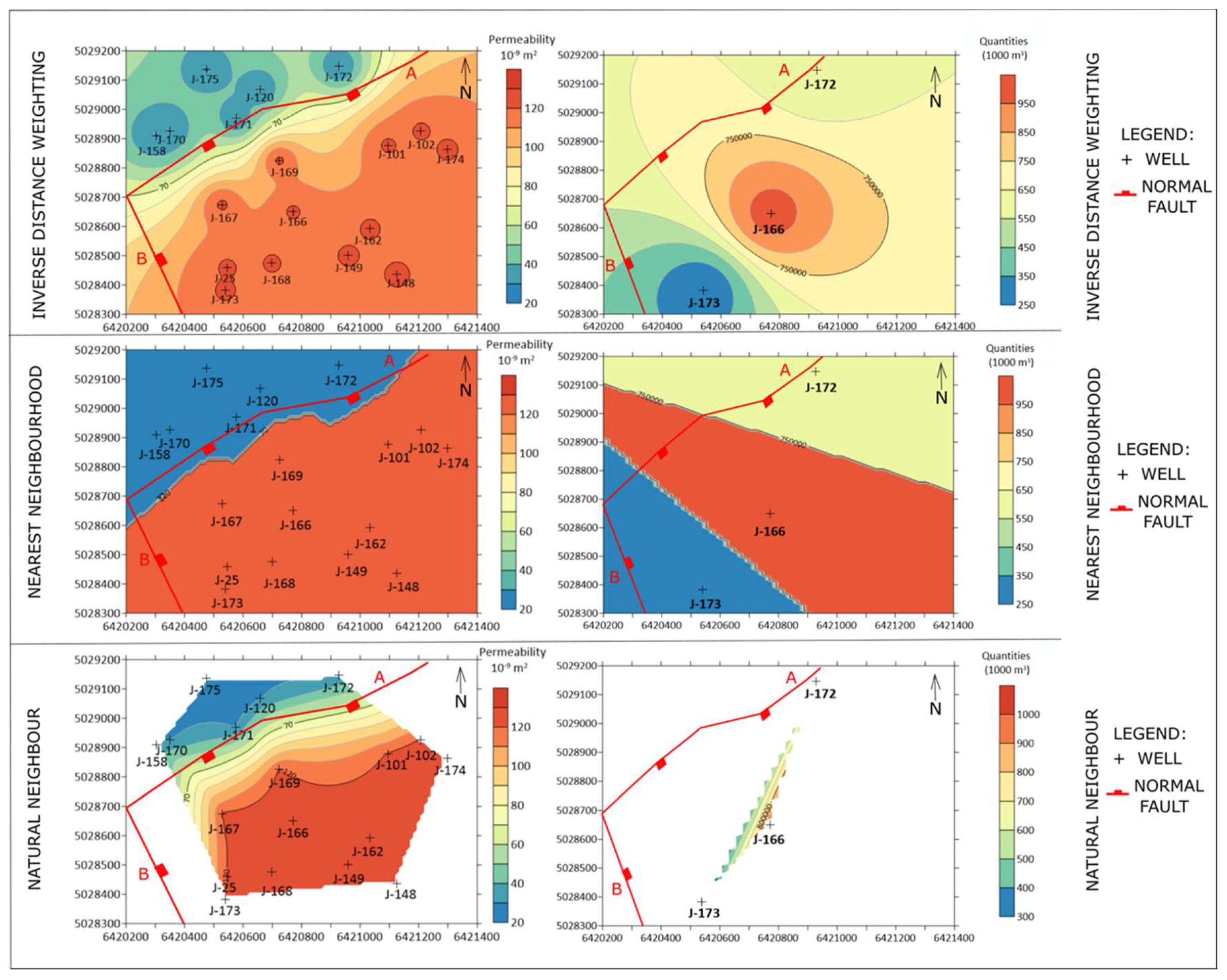
41] less than 20 inputs data. Furthermore, such datasets could be subdivided in groups with respect to the number of data inputs: a) 1–5, b) 6–10 and c) 11–19. One example is selected here when the reservoir mapping is done by mathematically simpler methods (compared with previously widely used kriging) and results are accepted as the best possible outcomes for further reservoir development. The permeability maps of the Lower Pontian “K” reservoir (Lower Pontian age, 18 data) of the field “B” are shown in
Figure 3.
All maps obtained with different methods (
Figure 3) are validated with a cross-validation (
Table 1) and visual assessment (where the larger “bull’s-eyes” areas mean worse interpolation).
Two interpolation (IDW, NaN) methods and one zonal (NN) method, gave different mapping results as well as cross-validation errors, as expected. Interestingly, each of them led to at least one useful information about analysed reservoirs, i.e., about connection between permeability and injected water volumes, including the role of some fault zone. The IDW method algorithm remains the main interpolation method of mapping for a small reservoir dataset in Northern Croatia. Other interpolation methods, NN, NaN, may be additional information. But the main advantage was that such datasets could be divided into three classes regarding their mapping, as follows: (a) 1–5, (b) 6–10 and (c) 11–19 inputs. The “class a” could not be analysed with the NaN method because it is often not possible to calculate the cross-validation and the interpolated area is very small regarding unit margins. In the “class b” and “class c”, all three methods gave results, and the main selection criteria could be cross-validation.
Malvić et al. [
40] also analysed the possibility of artificially increasing the input data set using the “jack-knifed” method. That is a resampling statistical technique, later upgraded into, e.g., bootstrapping. It is useful for statistics estimation, sequentially leaving out each value from datasets and calculating the statistical parameters of remaining data. For example, if the estimated parameter is the population mean (x), using jack-knifing it is possible to calculate the mean of each sub-dataset that includes all but the i-th measurement (x
i) using Equation (12):
where:
mean of sub-dataset, where i-th data is skipped,
- n
number of data points,
- j
data currently analysed.
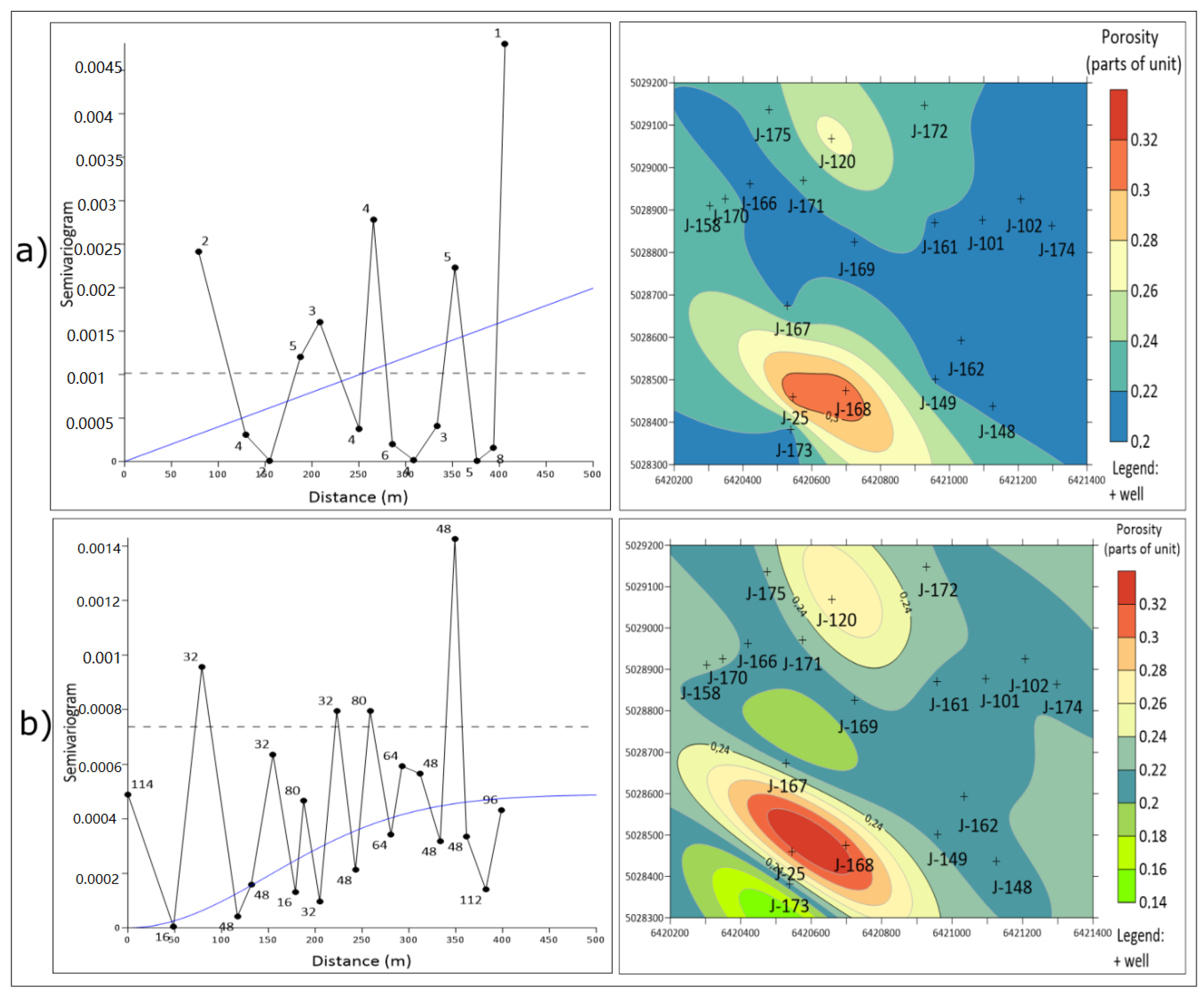
The presented analysis is the first of such a kind in the Sava Depression (Northern Croatia). It represents the continuation of previous geostatistical analyses conducted in that depression and the entire CPBS. The “jack-knifed” method was applied on porosity of reservoir “K” (19 data) of the “B” field (
Figure 4).
The porosity maps obtained were analysed by comparing the cross-validation values and expression of the “bull’s-eyes” effect. The results of the analysis of the “jack-knifing” method are summarized in
Table 2.
The results in
Table 2 confirm the possibility of applying the “jack-knifing” method to reservoirs with small data input and should be compared with the maps obtained by the IDW method. By contrast, in another analysed reservoir, the OK was not accepted as the interpolation method, but IDW has been accepted. It was the case when jack-knifing did not yield any progress in spatial modelling and the kriging has been abandoned as an approach.
The permanent problem of small datasets could be oversized with new data. Such data can be obtained with new sampling, but also with the creation of new artificial data, based on the statistical properties of original dataset. The jack-knifing is one such method, appropriate for datasets of 15–30 points, where the basic, descriptive statistics are more or less representative (variance and mean), and the Gaussian distribution can be assumed or verified with use of the Shapiro-Wilk test. In the presented analysis, the original semivariogram results were highly uncertain, with large oscillations, a small number of data pairs per class and unknown nugget. Consequently, the linear model was the only acceptable theoretical model to use. Due to fact that a small dataset could not be statistically representative, the new kriged maps interpolated from “jack-knifed” semivariograms has been tested (a) visually (maps without the “bull-eye” or “butterfly” effects are better) and (b) numerically, using cross-validation and comparing with the simpler method of the IDW. Obviously, the results were better in one of the two cases where such validation has been applied.
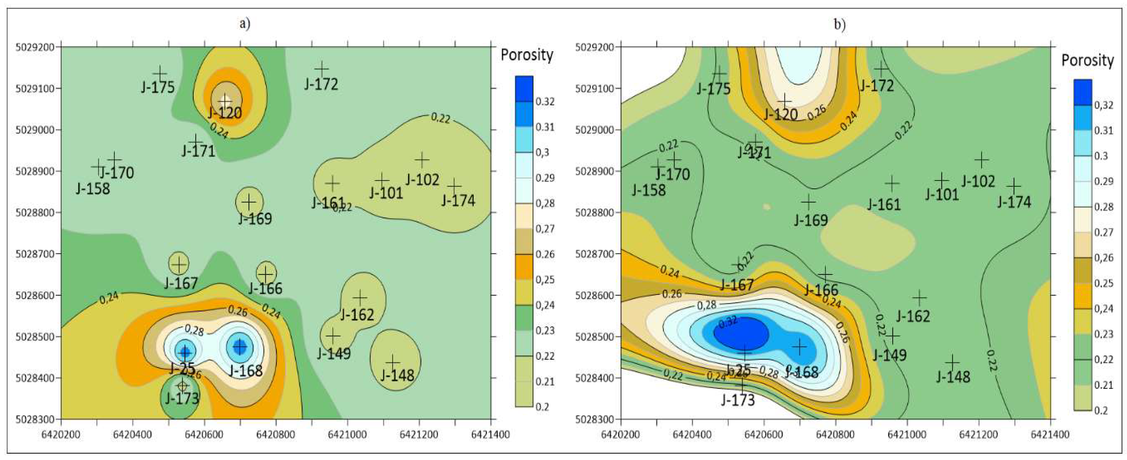
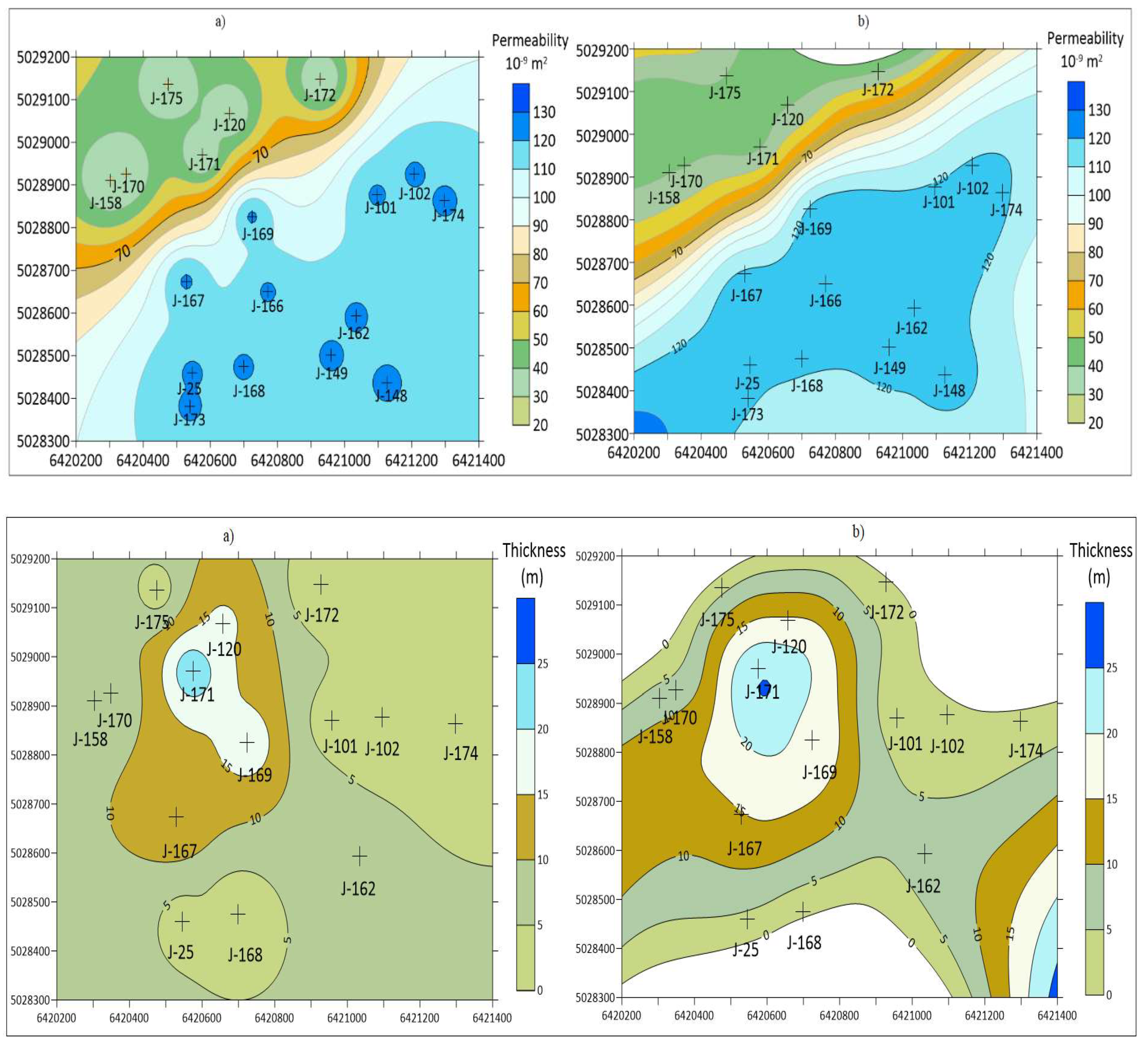
The next examples are taken from [
43] and compare the differences between the results obtained with the IDW and MSM methods. The IDW does not use weighting coefficient, i.e., each value is “weighted” by a simple (powered) inversely proportional distance from the measured point. The MSM (Modified Shepard’s Method) uses relative weights. The porosity, permeability and thickness maps, interpolated with IDW and MSM are given in
Figure 5. They show the oil reservoir “K” of the Lower Pontian age in the Sava Depression.
The maps obtained by the IDW and MSM methods could be assessed in two ways. One is numerical, using cross-validation. The another is quick-look searching for observable feature of highly expressed local value, i.e., bull’s-eye or butterfly shape effects. The expected advantage of the MSM is the larger smoothing of the shapes, which is confirmed in that analysis (
Figure 5). The numerical cross-validation strongly favoured the IDW (
Table 3).
The difference resulted from the different mathematical backgrounds of those two methods [
43], because the IDW takes into account all measured points or work with general searching radius (or radii for ellipsoid), but the MSM works with local searching by default. This is why cross-validation was higher for MSM—for porosity 289%, permeability 7%, and thickness 49%.
Both methods, obviously led to appropriate quick assessment of the reservoir. However, it was also shown that visual assessment is sometimes the more important criteria than purely numerical cross-validation, what is a crucial conclusion for subsampled reservoirs of the CPBS, and stressed the importance of human and geological expertise, and not purely the application of interpolation algorithms. Consequently, [
43] recommended the MSM for subsurface geological mapping of Neogene reservoirs in Northern Croatia in (a) number of samples smaller than 20 measured values, and/or (b) for early exploration phase or later development phase when the number of measurements of the selected property is small, but a quick insight in the spatial distribution of such variables is necessary.
4. Recent Advances in Biostatistics Applied in Palaeontology and Case Studies from Croatia and the Wider Region
Paleontological studies published by numerous authors, including those from Croatia, almost always include basic numerical analyses in recognizing the different taxa. In Croatia, [
44] measured the dimensions of the bivalve shells (length, width, length/width ratio of the shell, apical angle) in order to recognize the bivalve subspecies. In her dissertation and several published papers (e.g., [
45]), A. Sokač applied biometry in order to present the differences in growth pattern of male and female ostracods. One of the earliest graphically substantiated biometric analysis on the fossil assemblage from Croatia was published by [
46], who studied the taxonomy and biometry of Eocene corals. The authors distinguished two coral species based on the biometric analyses of the smallest and the largest diameter of the calyx, and the height of the coral calyx plotted in a scatter diagram. Looking at the dispersal of the measured parameters, two areas of dispersal could be recognized, indicating the existence of different species between measured specimens.
During the last decades, a number of global researches were focused on the paleoecology of terrestrial, fresh-water or marine biota. In Northern Croatia, Miocene deposits from the Paratethys epicontinental Sea comprise the marine invertebrate fauna, mostly foraminifers, mollusks and ostracods, which were often subject to biostatistics analyses (e.g., [
47,
48,
49,
50]). The following data, common in palaeoecological studies, are presented in the referred papers: plankton/benthos ratio, number of species, relative abundance of benthic species within the community, species diversity of benthic foraminifera estimated by the Shannon–Wiener index (H), dominance (D), Fisher α index (α), oxygen index and the infauna/epifauna ratio. The Shannon–Wiener index or Shannon diversity index (H) estimate the species diversity in the assemblage, as described in
Section 2.6 of this paper (after [
42]). Dominance (D) reflects a distribution of a particular species in the assemblage, and the dominant species are those presented with >10% in the sample [
42]. The Fisher α index (α) shows the relation of the number of species to the number of the individuals, and to explore the number of species by each individual, a log series distribution is used [
42]. This index is used for palaeoecological determinations, because specific values are characteristic for each environment. Depending on the index value range, we can analyse the palaeoecological changes in the environment.
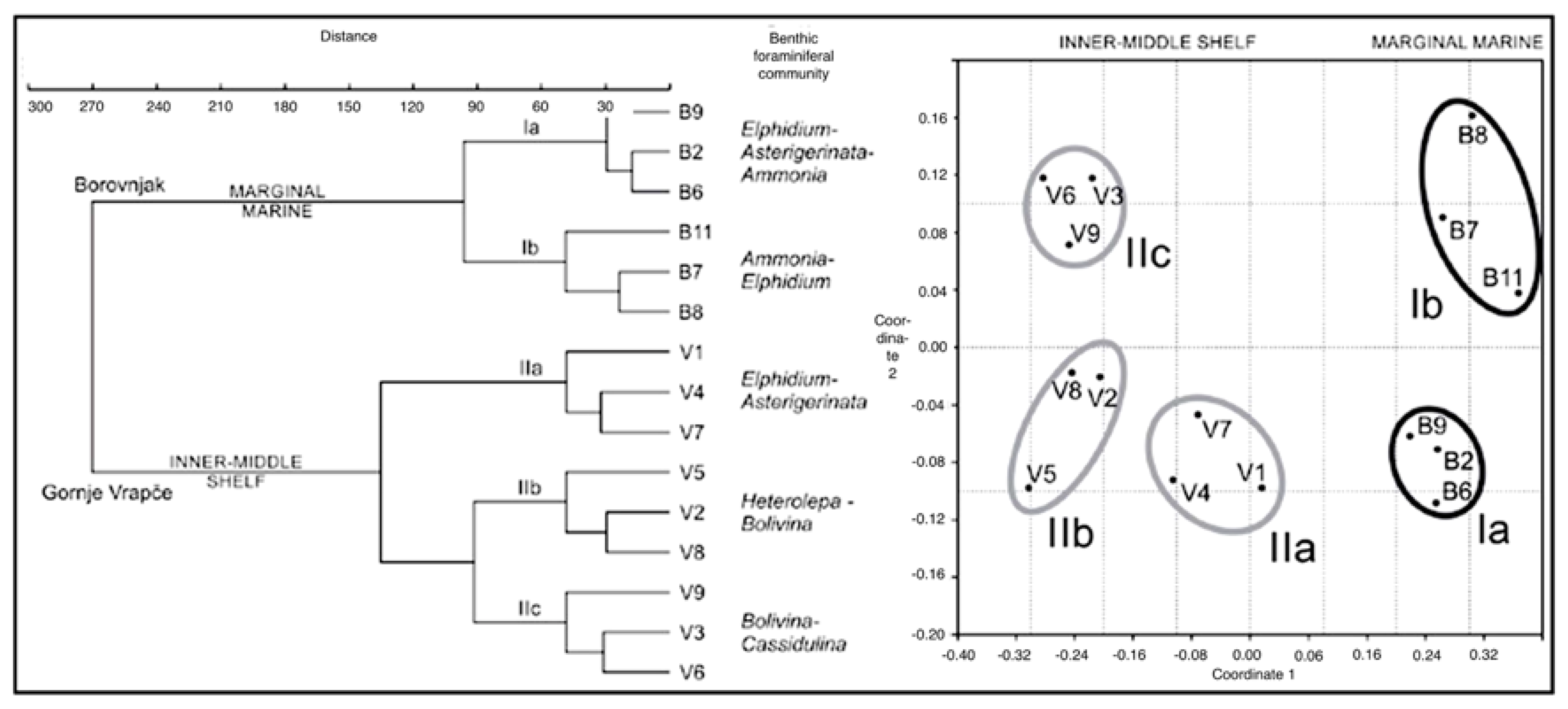
The aforementioned analyses were enhanced by defining and comparing the benthic foraminiferal fauna from different localities conducting the Cluster Analysis and Non-metric Multidimensional Scaling by means of the PAST (PAlaeontology STatistic) Program (
https://folk.uio.no/ohammer/past/; e.g., [
48];
Figure 6).
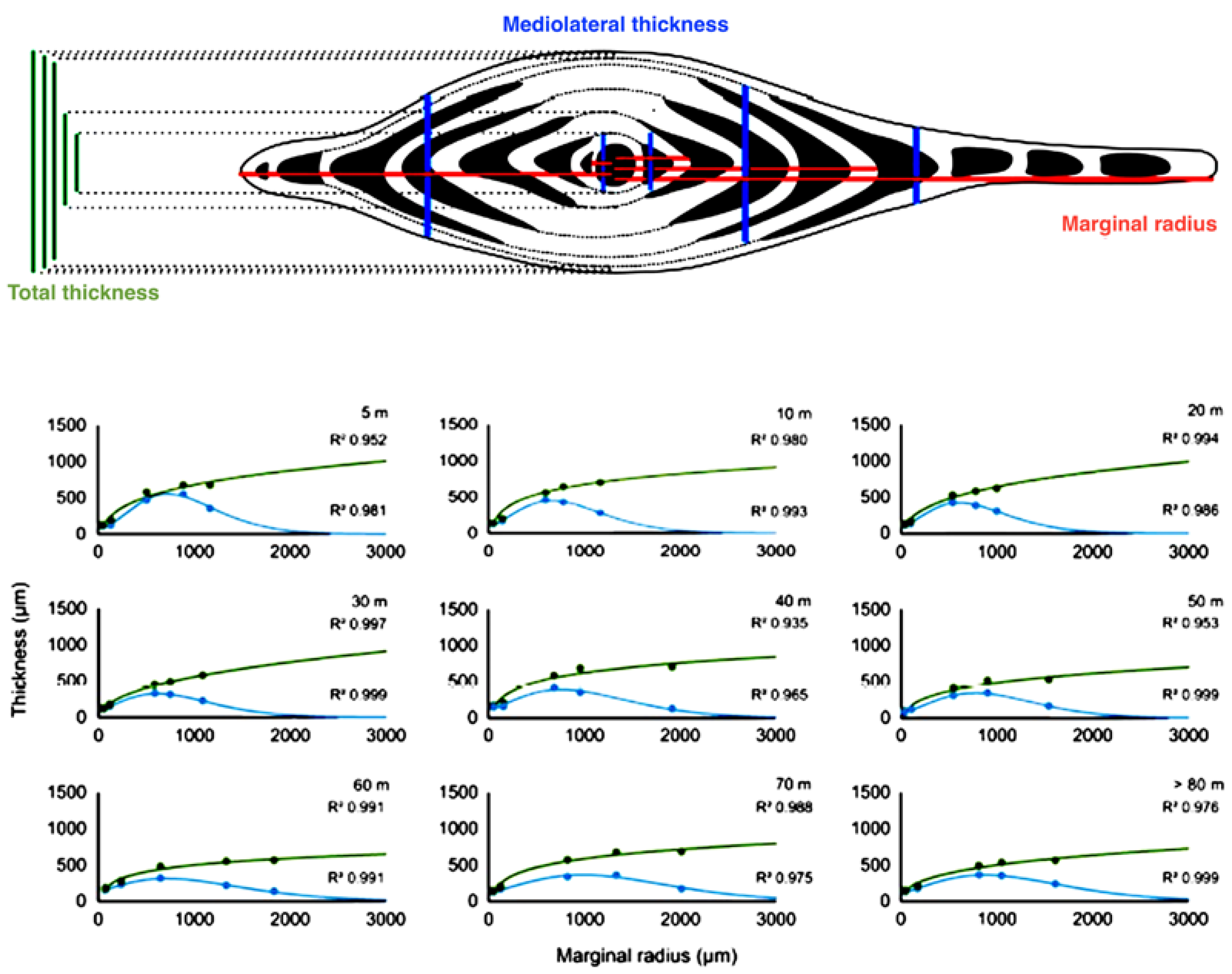
There are a number of other papers dealing with paleoenvironmental reconstructions of fossil communities based on the biometry of benthic foraminifera. Growth characteristics are used as a parameter for the palaeoecological and phylogenetical studies in the wider region (e.g., [
51,
52]). For example, [
53] calibrated test flattening of the foraminifera species
Heterostegina depressa as a bathymetric signal (
Figure 7), using its growth functions and thickness. Similar study can be applied to the Miocene large nummulitids from Northern Croatia.
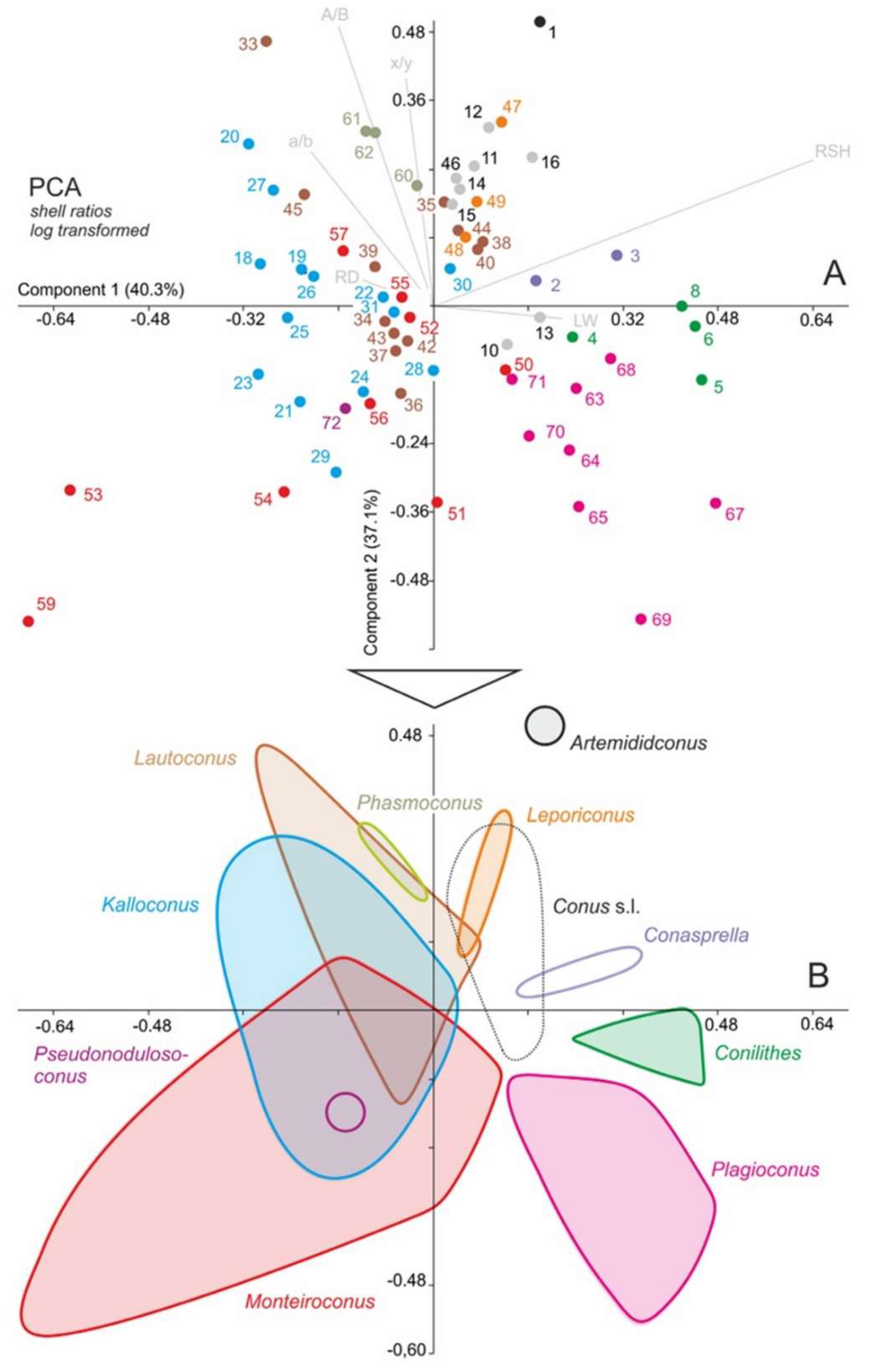
Biometric studies are also commonly applied in taxonomic study of mollusks. For example, a thorough revision based upon this method was made by [
54] on gastropod families Conidae and Conorbidae from the Paratethys Sea. The authors measured several shell parameters (shell length, maximum diameter, aperture height, height of maximum diameter, spire angle, apertural length, the angle of the last whorl, length width ratio, relative diameter ratio, position of maximum diameter ratio, relative height of spire ratio, subsutural flexure, mean and standard deviation), analysed by principal component analysis (PCA). Applying this analysis, authors compared similar species of Conidae and showed the separation of the species and morphospace occupied by genera (
Figure 8).
Studies from Croatia were mostly focused on gastropods and scaphopods (e.g., [
55,
56,
57]). Several parameters are measured (height and length of the shell, apical angle), defining the basic numerical data useful in species determination, morphometric characteristics of the group, correlation with recent species, comparison with other localities and palaeoecological interpretations.
Bošnjak et al. [
55] studied the Miocene planktic gastropods from northern Croatia and, based on the measured shell elements, compared their data with the available published measures of that fossil group found in the Miocene deposits of the neighbouring areas (
Figure 9).
Bioerosive traces on skeletal remains, in most cases traces of predation, are also rather common topic in biostatistical analyses. Measures and shapes of the drill-holes can indicate the possible predator and help to gain a better insight into the predator–prey relationship, as described in numerous papers (e.g., [
58] and references therein).
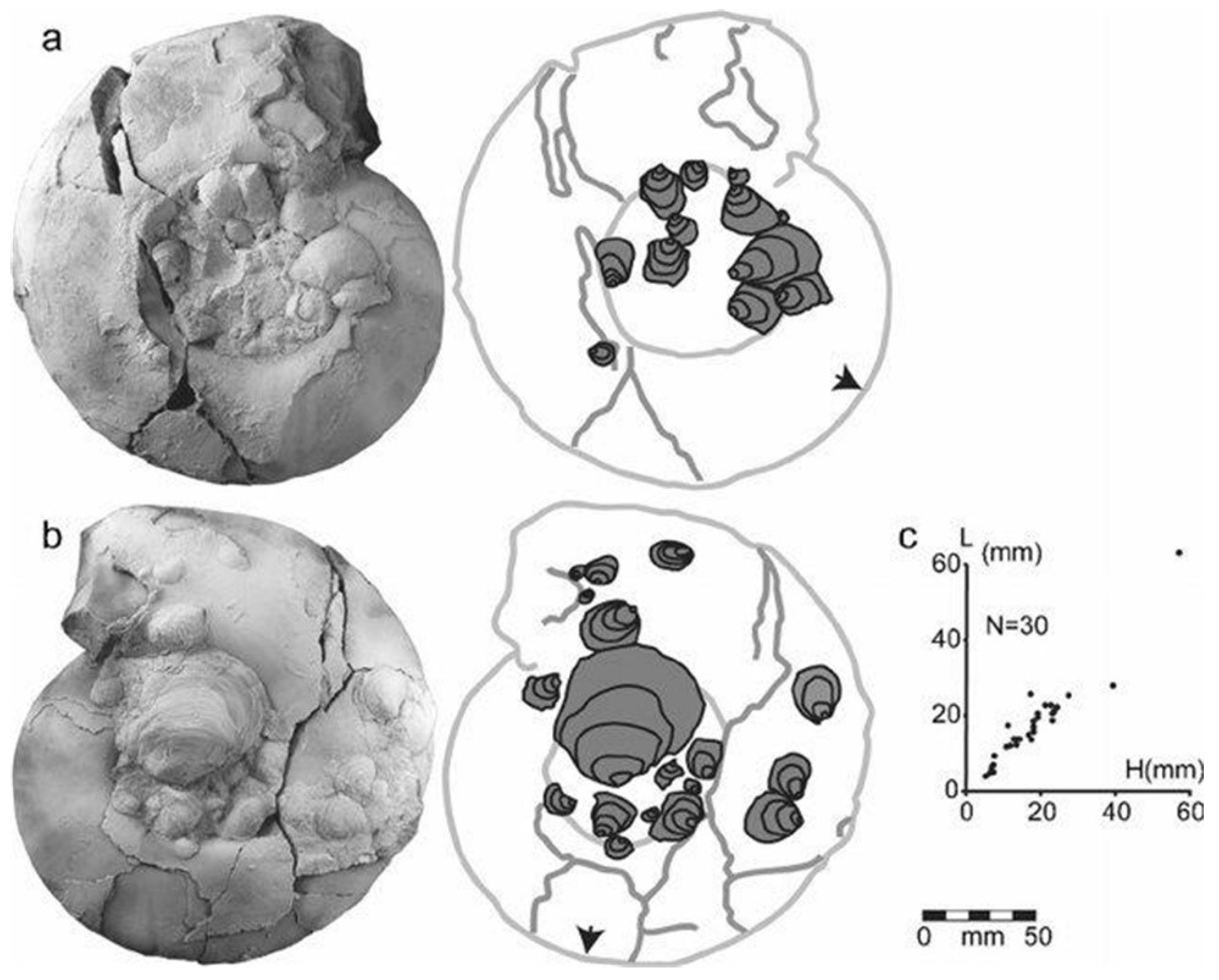
One more example of biostatistics analysis is presented in [
59]. The authors measured the orientations of oyster attachments on ammonite shells, concluding that the oysters attached themselves while the ammonites were living (
Figure 10). The results are helpful in palaeoecological studies of fauna in oxygen-depleted environments.
Biostatistical analyses are also common in studies of vertebrates. In Croatia, research included the study of dinosaur footprints. The measured parameters of footprints included width and length of the footprint, and length of the second, third and fourth finger (e.g., [
60] and references therein). These studies give an insight on the dimensions of the animal (height) and type of their movement (walking) based on the calculations of the movement speed (e.g., [
60,
61,
62,
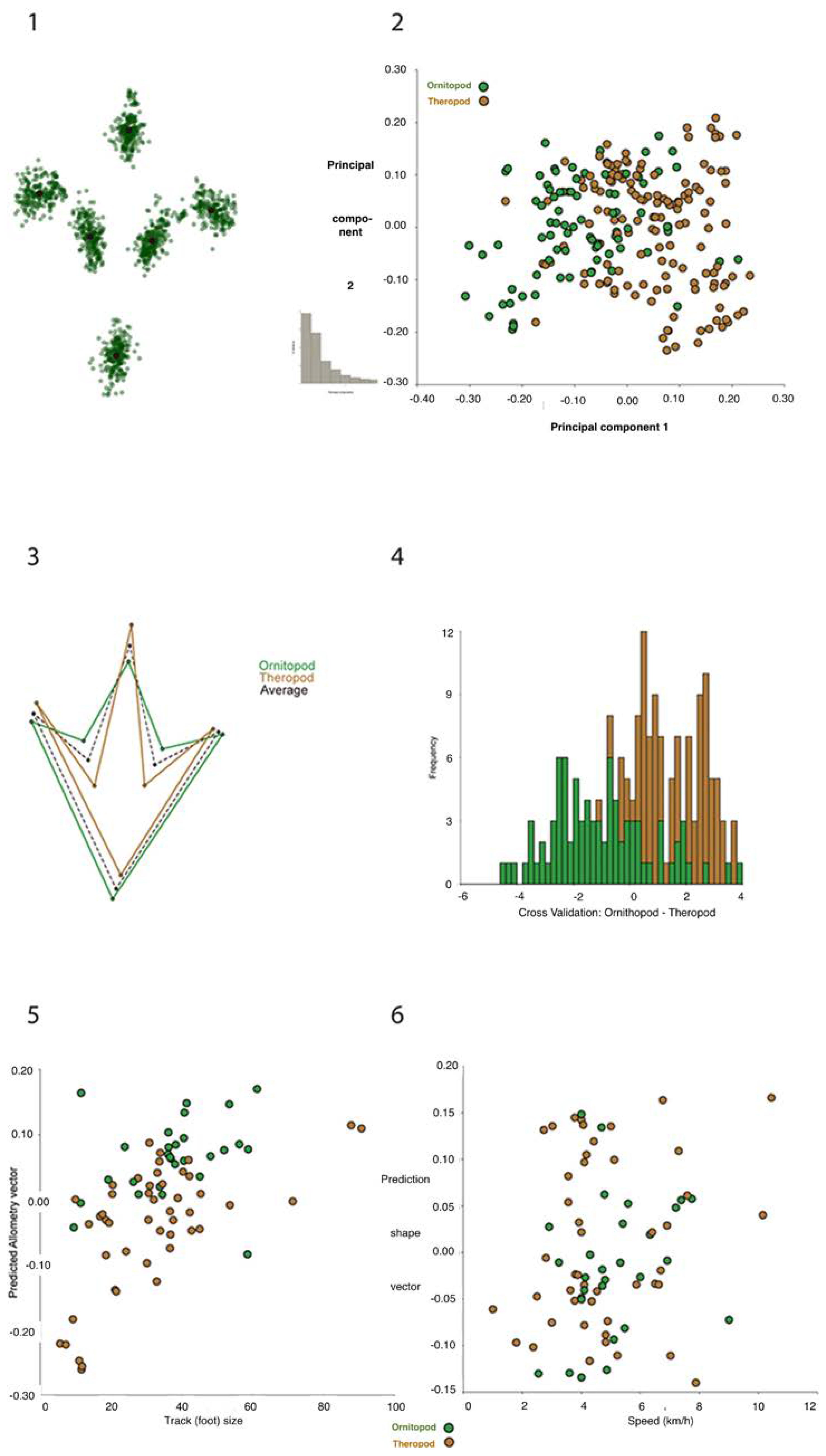
63] and references therein), which gives a better insight into the biodynamics of the animal. Costa-Pérez et al. [
64] demonstrated the application of geometric morphometrics as a tool for the shape analysis of the dinosaur footprints and trackways geometric differences (
Figure 11).
We can conclude that biostatistical analyses generally occurred very early in paleontological studies. In Croatia, their number exhibits the pattern of periodicity. Basic numeric analyses of fossil assemblages were published in the mid-1990s, marking the first peak of biometric studies in Croatia. The second peak was during the first decade of the 2000s, with most research done on microfossils (foraminifers and accompanying ostracods). We can say that the third pulse is happening from 2016 onwards, considering the various groups of fossil biota.
The analyses are mostly made to give more insight in the paleoecology of populations or fossil assemblages, and to help in the species determination. To present the analysed parameters, common statistical tools are used, mostly MS Office Excel and PAST (PAlaeontological STatistics) programs.
5. Discussion and Conclusions
The topic “Advances in Geosciences” is so broad that any publication would hardly cover only the small portion of significant milestones that shaped and led the progress in geosciences in general. The spectre of geosciences includes so many “fundamental” sciences that the means of progress are very different, regarding data, methods and problems. Geosciences could be found in social (e.g., geography), technical (e.g., geodesy) and natural (e.g., geology) sciences. This is why the authors selected only one science (geology) with only one small segment (subsurface and surface geology) and tiny analytical, numerical methods (small datasets in mapping, larger in biostatistics). Even in such a case, the presented cases are given mostly from the researching area where authors worked mostly in the last decade, i.e., original samples taken from the surface and subsurface of the Northern Croatia.
However, both examples present the areas where, at least in Croatia, huge progress was made and referencing methods for later researchers were set up. After more than 15 years of extensive and successful application of the different Kriging techniques in the subsurface mapping of the CPBS, the problem of a small dataset where geostatistics cannot be reliable applied has been solved. Several simpler algorithms are tested, validated and recommended for application, namely inverse distance weighting, nearest neighbourhood, natural neighbourhood and the modified Shepard method. For such small datasets, the importance of mutual application for cross-validation and visual assessment had been stressed. Additionally, the Kriging was simultaneously tested as an alternative to such algorithms, even in cases when variogram model cannot be calculated as reliable value, even an omnidirectional one. The extensive experiments with the jack-knifing method have been done on variogram, creating artificial data from original dataset. In some cases, jack-knifed variograms gave competitive value to the kriging results, but geostatistics was eliminated as the first choice in mapping analysis of small subsurface datasets.
The application of biostatistics has been presented on very different samples, collected from shallow subsurface or surface outcrops. Here the numerical values characterised not petrophysics, but morphological variables of different fossil groups (foraminifers, molluscs, vertebrates). In the presented examples on molluscs, parameters like the height and length of the shell are measured giving a set of numerical values for determination of morphometrics and consequently species which gave more insight into Miocene palaeoecological conditions and environments in Northern Croatia, especially during the existence of the Paratethys Sea. On a larger scale, biostatistical analysis in Croatia helped to reconstruct the size and height of, e.g., dinosaurs, using footprint measurements. Two periods of the Croatian biostatistical (biometric) analyses, presented with relevant publications, are noted. The first was in the mid-1990s, and the second was during the first decade of the 2000s, with most research done on microfossils (foraminifers and accompanying ostracods). Croatian researchers entered the third fruitful period from 2016 onwards, currently analysing the various marine fossil biota aiming to determine species and their paleoenvironments.
Both examples showed the useful application of geomathematical tools in geology. The first group showed how small datasets (n < 10 data) of different geological variables collected in the Neogene sandstones in the Northern Croatia can be reliably mapped with the IDW and MSM methods. The second presented how morphometric and surface features could be collected, numerically analysed and applied in paleoenvironmental reconstructions. Uncertainties, of course, remained due to the data properties. The most problematic is clustering, which can be hardly handled when datasets are small and/or spatially noisy. In such cases, two crucial statistical properties cannot be reliably checked or established. That are proof of the normal distribution and statistical representativeness of a dataset (mean, variance of population). However, the results, carefully validated and correlated with other, non-numerical (indicator, categorical) geological knowledge, are of great help in creating better geological models.

 ,
, 


