Observational and Critical State Physics Descriptions of Long-Range Flow Structures

Abstract

Using Fracture Seismic methods to map fluid-conducting fracture zones makes it important to understand fracture connectivity over distances greater 10–20 m in the Earth’s upper crust. The principles required for this understanding are developed here from the observations that (1) the spatial variations in crustal porosity are commonly associated with spatial variations in the magnitude of the natural logarithm of crustal permeability, and (2) many parameters, including permeability have a scale-invariant power law distribution in the crust. The first observation means that crustal permeability has a lognormal distribution that can be described as $\kappa \approx {\kappa }_0\exp \left(\alpha \left(\phi -{\phi }_0\right)\right)$, where α is the ratio of the standard deviation of ln permeability from its mean to the standard deviation of porosity from its mean. The scale invariance of permeability indicates that αϕ_ο = 3 to 4 and that the natural log of permeability has a 1/k pink noise spatial distribution. Combined, these conclusions mean that channelized flow in the upper crust is expected as the distance traversed by flow increases. Locating the most permeable channels using Seismic Fracture methods, while filling in the less permeable parts of the modeled volume with the correct pink noise spatial distribution of permeability, will produce much more realistic models of subsurface flow.

1. Introduction

As discussed by Sicking and Malin (2019) [1], new methods of passive seismic data acquisition and processing allow ambient subsurface fluid connectivity to be mapped. Complementary to the information on fluid pathways from microearthquakes (MEQ) generated by massive high-pressure (active) fluid injections (e.g., [2]), the new passive technique of Fracture Seismics (FS) can directly reveal both the locations and relative permeabilities of fluid-filled fractures. Further, and perhaps more importantly, passive FS mapping shows the degree of flow connectivity at distance scales greater than a few tens of meters from the point of active fluid injection.

A variety of independent evidence indicates that locations where MEQ and FS activity is most intense are where fluid flow is most likely [1]. FS maps typically reveal long connectivity structures that conduct fluid flow, as illustrated in Figure 1. The top panel shows the intensity of FS signals, and the bottom panel indicates the fracture-connectivity skeletal pathways through the cloud where FS signals are most intense and fluid flow is most likely.

The FS pattern in Figure 1 is from a fracture stimulation in the Marcellus gas shales, and the connectivity of its permeability-related signals may be considered a surprise. However, in this case the FS flow prediction was confirmed both by gas pressure communication and by a tracer experiment. These measurements showed a high degree of connectivity over ~600 m between vertical Well B and horizontal Well A, as indicated by the FS backbone in the lower panel. This backbone was observed in the FS data from Stage 3, and then later also at Stage 4, in advance of the arrival of tracer signals in Well B, which appeared at the time Stage 5 was stimulated.

There are good observation-based theoretical reasons to expect the kind of spatially extended crustal flow connectivity on the hundred-meter scale seen in Figure 1. The purpose of this paper is to discuss these reasons. We show that the distribution of features observed in such FS maps is expected. The expectation that crustal fluid flow over length-scales >10–20 m will be through high-connectivity flow structures is discussed below, from both (a) direct observations and physical logic and (b) the power law scale invariance in the observed self-similarity of fracture-connectivity patterns. The first approach was developed over the last three decades in a series of papers (e.g., [4,5,6,7,8,9,10]). The second approach has a vast and densely spaced literature (e.g., [11] and the many references therein). Our purpose here is to bring these insights together and convey an understanding of how upper-crustal fluid flow is likely to be structured, based on observations and the critical state physics of brittle rock.

2. Crustal Observations and Implications

2.1. The Observed Relationship between Crustal Porosity and Permeability

This section first shows that spatial variations in crustal porosity invariably coincide with commensurate spatial variations in the natural logarithm of permeability. It then shows that this means that the magnitude of crustal permeability commonly has a lognormal distribution, even though the magnitude of porosity that is spatially associated with permeability is normally distributed. Following Leary et al. (2017, 2018) [12,13], we derive a general expression that encapsulates this observation and deduction. The derivation shows that the combinatorial probability of crustal pore and fracture connections provides a logical explanation for why normally distributed pores are associated with a lognormal distribution of permeability. There could be a physical extension between pores and fractures [13] which we do not discuss here. With increasing strain, broken grain cements could progressively localize deformation, eventually leading to faulting, for example. This is not addressed in this paper. Here, we use observations of cores to discuss the connection conditions for permeability and learn how a normal distribution of pores and pore connections leads to the observed lognormal distribution of core permeability. We then transfer this insight to fractures.

Figure 2, Figure 3 and Figure 4 show field data that illustrate how changes in crustal porosity are invariably associated with changes in the natural logarithm of permeability,

$$\delta \phi \propto \delta \ln \kappa$$

(1)

The (possibly irregularly spaced) porosity and permeability values in these figures were measured down well-core samples according to standard oil-field procedures (e.g., [14]). The histograms on the left side of Figure 2 show that the porosity values of four North Sea cores have a normal spatial distribution, whereas the permeability values have a lognormal distribution. Similar histograms of porosity and permeability are shown in Figure 3 and Figure 4.

On the right side of Figure 2, the porosity and permeability values are plotted as a function of sample number. In Figure 3 and Figure 4, they are plotted as a function of sample depth. The measurements are plotted in normalized form, such that their variations have zero-mean and unit variance. This is achieved by subtracting the mean porosity (or ln permeability) and dividing by the standard deviation of porosity (or ln permeability). These profiles show that where there is a change in porosity there is a correlated change in ln permeability. Natural logs are used throughout the discussion for consistency with these observational plots and for compatibility to theory.

Whereas the number of samples with small porosity values rapidly decreases in these histograms, the same is not true for permeability histograms. The roll-off in the number of samples with small permeability values can be seen only in the plot of numbers versus the logarithm of permeability, and may be due to failure to measure variations in low permeability. The potential for undersampling suggests that the permeability distribution could be alternatively described as a power law (which has no roll-off at low permeability) instead of lognormal. Both logarithmic and power distributions are long-tailed at the high permeability end of their distributions. However, power distributions are fat-tailed, meaning this distribution has more high permeability values than a lognormal distribution.

The important point here is not these differences between power and lognormal distributions, but simply that, on simple inspection, the porosity and permeability distributions are normal and lognormal, respectively, and these relationships are general. The Figures show data from wells worldwide. They depict the most commonly observed characteristic of reservoir rock porosity and permeability. Furthermore, the normal-versus-lognormal correlations between porosity and permeability are not dependent on the orientation of the sampling well. Figure 4 shows that the same relationship is observed in cores from a horizontal well as in cores from vertical wells. Be it a vertical or horizontal well-core sampling sequence, the differences in their population distributions remain the same: normally distributed porosity and long-tail power permeability. Both these distribution and correlation relationships appear to apply just as well along rock formations as across them.

Figure 2, Figure 3 and Figure 4 show data that establish Equation (1). Equation (1) can be integrated to yield an expression between the spatial variation of permeability, κ(x,y,z), and the spatial variation of porosity, φ (x,y,z)

$$\kappa \approx {\kappa }_0\exp \left(\alpha \left(\phi -{\phi }_0\right)\right),$$

(2)

Here, ${\kappa }_0$ and ${\phi }_0$ are the mean values of permeability and porosity, and α is a constant of proportionality. That (2) follows from (1) can be easily verified by differentiating (2) with respect to $\phi$. If $\phi ={\phi }_0\pm {\sigma }_{\phi }$, it follows from (2) that $\ln \kappa =\ln {\kappa }_0\pm \alpha {\sigma }_{\phi }$, where $\alpha$ is the ratio of the standard deviation of $\ln \kappa$ to the standard deviation of $\phi$:

$$\alpha ={\sigma }_{\ln \kappa }/{\sigma }_{\phi }.$$

(3)

When α is very small, the series expansion of the exponential in Equation (2) reduces to a linear relationship between the departure of $\kappa$ and the departure of $\phi$ from their mean, and both permeability and porosity are normally distributed. In the small-$\alpha$ limit, permeability equations such as the Kozeny–Carmen relationship hold. In this domain, the flow is homogeneous for a normal distribution of porosity.

When $\alpha$ is large, $\kappa$ fits the definition of a lognormal variable, where the permeability distribution has a long permeable tail. In the large-$\alpha$ limit, $\ln \kappa$ has a standard deviation spread of ${\sigma }_{\ln \kappa }$. If this spread is large enough and, as discussed in the next section, the spatial distribution of permeability is a power distribution, the flow will be channelized. These two conditions (large $\alpha$ and a power spatial distribution of permeability) for channelized fracture flow are what we investigate in this paper.

2.1.1. The Connection–Condition Explanation for a Lognormal Distribution in Permeability

The reason that a normal distribution in porosity magnitude can lead to a lognormal distribution in permeability magnitude can be understood if it is recognized that permeability requires a connection condition to be met. For the current discussion, this connection condition is that fractures (or pores) must be able to pass fluids onward to other fractures (or pores).

Shockley (1957) [15], among others, illustrated how physical/statistical observables (events) that are normally distributed can interact conditionally to create other observables (events) that are lognormally distributed. His simple example asked why relatively few authors publish the bulk of scientific papers. He proposed that eight author traits are necessary to produce a publication: (1) ability to select problems; (2) competence to work on them; (3) ability to recognize a result; (4) ability to prepare a manuscript; (5) ability to present results adequately; (6) ability to profit from criticism; (7) determination to submit a manuscript; and (8) ability to respond to referees’ criticism. Assuming each author trait is normally distributed through a population of scientists, the conditional nature of the final ‘event’, the publication of a scientific paper, depends on the product rather than the sum of the component traits. If p₁ is the probability for trait 1, p₂ for trait 2, etc., then P = p_1* p_2*…* p₈ is the probability of publication, and only a few authors will possess all the traits needed for successful publication. Successful authors will be rare, and the distribution of author publications will have a long tail: few scientists meet the connection condition of having all eight traits, so they publish a disproportionate share of scientific papers.

Permeability requires that pores and fractures be connected. As the scale or volume of interest becomes larger, there will be more and better connections between pores, and longer and more permeable fractures within a given volume, and the probability that some subset of pores or fractures will be connected will increase with increasing volume. For example, given n independent fractures in a volume, simple counting shows there are n! = n_* (n-1) _* (n-2) _* ways to connect them. If the number of pores or fractures increases by δn, the probability of connection will increase: δln(n!) = ln([n+δn]!) − ln(n!) ≈ δn ln(n). Since ln(n) changes more slowly than n, it is reasonable to assume that δln(n!) ∝ δn Associating n with φ, and n! with κ, we find δln(κ)∝ δφ, as shown in Equation (1), above. We thus see that, if permeability is viewed in terms of connections of pores or of fractures, it follows that a change in the number of pores (pore connections) or in the number of fractures will lead to a change in ln permeability.

2.1.2. Spatial Properties at the Critical State

Critical state physics principles can account for how variations in permeability become distributed spatially. This distribution is the second and final piece of information needed to determine whether the departures of ln permeability from its mean will lead to flow channeling.

One example is the application of critical state physics to the phenomenon of opalescence. Opalescence is the clouding of an otherwise clear liquid such as CO₂ at its critical temperature and pressure. Observed almost 200 years ago, this phenomenon was understood 100 years later to be related to spatial optical index fluctuations in the critical liquid which scatter light, thereby clouding the liquid. In the last 50 years, the amplitudes of these fluctuations have been found to be power law distributed as a function of their physical length scale. The longer the length scale of the fluctuation, the larger the amplitude of its density change. For example, if the density variations were decomposed into their Fourier components, the longer wavelengths would have a greater amplitude. The square of the amplitude might vary as 1/k, where k=2π/ λ, where λ is the wavelength of the Fourier component.

Properties that vary spatially in a power law 1/k fashion are scale invariant in the sense that you cannot deduce scale in an image of the material that contains the property. In the case of opalescence in a clear liquid, the pattern of optical index variations captured in a photo frame of tenths of a millimeter on a side looks the same and is statistically the same as that captured in frames that are millimeters on a side. Furthermore, the onset of density variations and the clouding they cause is related to a “structure function” such as ε = (T – T_c)/T_c, where T is the system temperature, and T_c is the critical point temperature (e.g., [16]). Importantly, the opalescence is clearly related to the proximity to the critical point and not to other properties of the fluid.

The critical-state percolation model [17,18] provides additional insight. In the simplest version of a percolation model, nodes in a square grid are connected to their neighbors by bonds that are either open (and allow flow between nodes) or closed (and allow no flow). If open bonds are randomly assigned according to some probability, there is a critical fraction of open bonds at which at least one pathway of conducting bonds spans the sample. Near this critical sample-spanning fraction, percolation model properties such as permeability, electrical conductivity, and diffusion coefficient are found to be power functions, and universally depend more on spatial dimension than the morphology (internal construction) of the medium [18]. This potentially greatly simplifies understanding rock properties. The flow backbone in the sample-spanning cluster is found by deleting all the dead-end conducting bonds where no flow occurs. The flow backbone provides a basis for the depiction of backbone fracture seismic flow structures shown in the bottom section of Figure 1. Note that the seemingly dead-end backbones of flow in Figure 1 could connect to overlying or underlying depth slices through the volume, or could discharge into a broadened flow.

2.1.3. The Critical State of the Earth’s Crust

A major insight of the late 20^th Century in the Earth Sciences is that the earth’s crust is stressed by plate tectonic forces, such that it is in a state of constant incipient failure [19]. The brittle crust is riddled with fractures that are always at or near mechanical failure. Fractures are power scaling or scale-invariant characteristics of rock [11]. Geologists must place a hammer or some other object of known scale in a picture of veins or fracture traces to indicate their scale (e.g., [11]). Leary et al. (2018) [13] have shown that the αφ₀ parameter in Equation (2) above, plays the same role in the deformation of the earth’s crust as the critical temperature plays in opalescence. If αφ₀ is between 3 and 4, the crust is in a state of constant incipient failure. The result is that the spatial distribution of fractures is power law, and it follows that the spatial distribution of permeability is power law. Barton, Camerlo, and Bailey, 1997 [20] have shown that the distribution of fracture trace lengths is also power scaling. Leary et al. (2018) [13] show that αφ₀ is between 3 and 4 for a wide variety of sedimentary rock, which means that they are in a state of incipient failure.

2.1.4. The Power Exponent of Permeability

Prior to the invention of FS methods, it was not possible to image fracture permeability directly to determine its location and spatial distribution. However, permeability proxies such as the mineral alteration caused by fluid flow through fractures and the size distribution of microearthquakes, can be used to infer the power exponent that characterizes the spatial distribution of fractures in rock [11]. The permeability power exponent can also be inferred from Equation (2) for a pink noise spatial variation in porosity or by the direct field mapping of fractures.

Figure 5 shows how the square of the amplitude (spectral density) of well-log measurements of fracture density, porosity, and fluid-flow-related mineral alteration fall off as the spatial scale of measurement (frequency) decreases. The variation in signal strength with depth, measured by well-logs, is Fourier transformed. The logarithm of the square of the amplitude (fluctuation power of the signal, S(k)) of each Fourier component is plotted against the logarithm of the spatial frequency, k, of the component measured in cycles/km (or any other units of measure, since the log slope is not affected by the units). The spectral density method is well described by Malamud and Turcotte (1999) [23]. All the properties related to fluid flow, plotted in Figure 5, show approximately a pink noise, scale invariant, 1/k power distribution.

2.1.5. The Flow Significance of the Distribution of Permeability

Figure 5 shows that down hole log measurements related to flow in fractures are power-scaling with an exponent of approximately −1:

S(k) ∝ 1/k^β, where β = 1.

(4)

This value of the power exponent, β, is intermediate between zero slope of randomly distributed white noise and the slope of two of red noise (the Brownian noise, obtained by taking the running sum of randomly distributed spatial properties). A power spectrum with a slope of one is called a pink noise. Equation (4) shows that, for pink noise, when k becomes smaller (e.g., the number of Fourier cycles per km is fewer and the variation extends over a larger distance), the signal power increases. For a pink noise spatial distribution of permeability, as the volume of rock becomes larger, it is increasingly likely that a permeable channel will short-circuit flow across the entire observed volume. We show this below by first discussing how white and pink noise distributions of porosity differ, and then use Equation (2) to convert a pink noise porosity distribution to a pink noise permeability distribution and address channeling.

Figure 6 contrasts white and pink noise distributions in porosity. The plots on the left side of Figure 6 depict a hypothetical white noise porosity distribution. The top image is a depth slice map of porosity. The middle plots the porosity along an arbitrarily directed hypothetical well-log through the depth slice map shown above. The Fourier power spectrum S(k) of this porosity well-log is plotted as a function of wave number k on the abscissa in the bottom image. The white noise is generated from a standard pseudo-random number generator in Matlab computational software.

The working assumption behind the white noise application to crustal randomness is that, at some suitably large scale-length, whatever is physically happening at one point in the formation is independent of whatever is happening at any other point. That is, above a suitable scale length, crustal flow structure is uncorrelated. The white noise uncorrelation assumption is inherent in the representative elementary volume (REV) method of crust flow modelling (e.g., [24,25,26]). Whatever the pattern in the REV, it is assumed that one could make a 3D rubber stamp of the REV and replicate the pattern at a larger scale by filling in the whole volume with the stamp. The largest and smallest features remain the same, no matter how many times a pattern is repeated or how large its volume is. REV patterns cannot increase or decrease the range of properties beyond those in the REV. REV’s thus have no scaling larger or smaller than that contained within the REV itself. As a consequence, the entire crustal flow volume is described by just one REV sub volume. There is no large-scale variation in permeability in the depth slice white noise map (top right).

In contrast, the 1/k spectrum pink noise-correlated spatial distribution of porosity is illustrated on the right side of Figure 6. The pink noise distribution of porosity is generated using discrete Fourier transform methods, as described in ([23], p.35). The pink noise porosity distribution is then shown along a hypothetical well-log through the depth slice image (middle right diagram) and plotted in power spectrum form in the bottom right image. The pink noise porosity distribution reveals different intensities at every scale length contained in the volume. The plan map shows dramatic inhomogeneities which connect over large distances. A yellow to red band across the entire property map can be seen in the middle of Figure 6, for example. This porosity pattern suggests that a flow channel could pass fluid across the entire image. In contrast to the uncorrelated plan map depiction to the left, no small portion of the correlated map is representative of any other small portion. The porosity level and pattern at one location cannot be used to predict what will be found in another small portion of the image. The spatial fluctuation power spectrum has a power slope of ~1 rather than ~0. Connected flow paths are expected, but the position of the spatially correlated pore-connectivity cannot be predicted on the basis of a limited number of samples.

The tendency towards channelized flow at large scale for a 1/k pink noise porosity distribution is demonstrated in Figure 7. Flow in this figure is calculated for a porosity distribution derived from a normal distribution of pore sizes with a 1/k power spatially correlated distribution with a power scaling exponent of −1, in the same fashion as described above. The porosity normal distribution is converted to permeability using Equation (2), a pressure gradient is imposed across the spatial permeability distribution, and the resulting flow is computed using the Matlab finite-element partial differential equation solver. The 2D grid has 300 × 300 element resolution. Arrows show both the distribution of velocity magnitudes and flow directions in the model domain. The ±2 spread in the natural logarithm of the flow velocity (ln|V|) in Figure 7 approximately matches the spread of natural log permeability shown in Figure 2, Figure 3 and Figure 4. The flow directions show that spatially correlated porosity leads to flow dramatically channeled across the model from the high-pressure boundary to the low-pressure boundary.

2.1.6. The Power Exponent of Permeability from Two-Point Analysis of Permeability

Figure 2, Figure 3 and Figure 4 suggest a mean value of ϕ = 0.2 ± 0.1. Assuming a critical state crust with αϕ_o = 4, it follows that α = 20, and, since $\alpha ={\sigma }_{\ln \kappa }/{\sigma }_{\phi }$, ${\sigma }_{\ln \kappa }$= 2, then whether ln κ has a 1/k crustal scaling can be tested by two-point spatial correlation methods. This analysis shows a power law separation exponent of −0.5. This corresponds to a Fourier power spectrum slope of 1/k for the ln permeability field [10,27].

2.1.7. Power Law Exponent of Permeability from Microearthquake Distributions

Over 18,000 m³ of water was recently injected at ~6 km depth in Finland to stimulate flow for deep geothermal heat extraction [28]. Over 54,000 microearthquakes (−1 < M < 1.9) resulted from this stimulation, of which 6150 were located and characterized. These events have a two-point correlation power law separation radius exponent of between −0.5 and −0.6 [10], which corresponds to a Fourier power spectrum slope of 1/k.

2.1.8. Power Law Exponent from Field Mapping of Fractures

Barton (1995) [11] reported on outcrop fractures mapped at 17 locations at scales from centimeters to kilometers. He found that fracture length had a fractal dimension of D~1.5.(range 1.4 and-1.7) Since fractal dimension is related to the exponent β as 2β = 5-2D ([23], p30), Barton found β ~ 1 from outcrop mapping. A β = 1 corresponds to a 1/k distribution, since, by convention, β is the negative of the exponent of k.

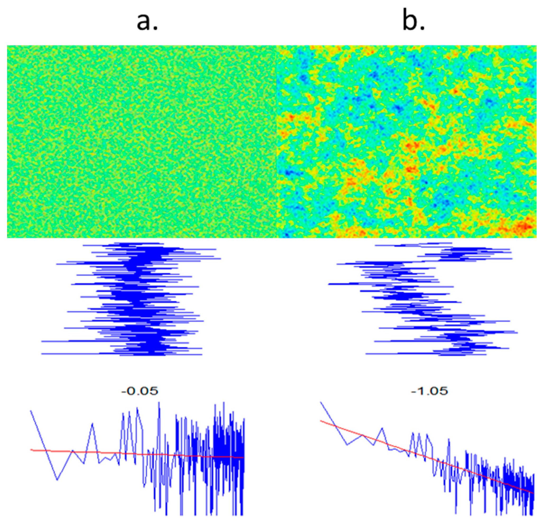
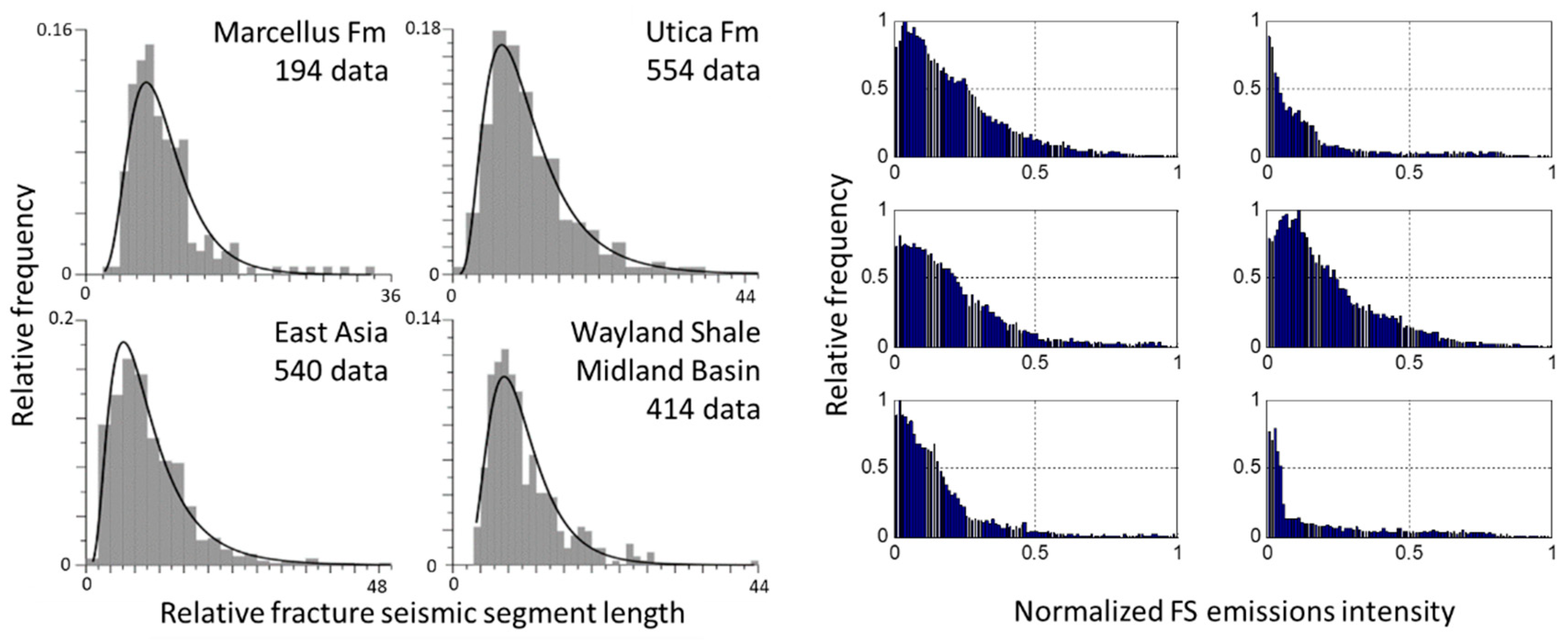
2.1.9. Power Exponent from Analysis of Fracture Seismic Images

The flow backbone shown in the bottom image of Figure 1 consists of connected linear segments with different levels of fracture seismic emission intensity and physical length. Histograms can be made of both relative fracture seismic segment length and FS emissions intensity, and their statistical distributions determined. Figure 8 shows that both of these properties have lognormal (or power law, since the roll over may simply reflect the limits of segment resolution) distributions, in which there are long fracture seismic intensity segments, and high FS emissions intensities that fall far outside of normal distributions, i.e., these distributions have long tails.

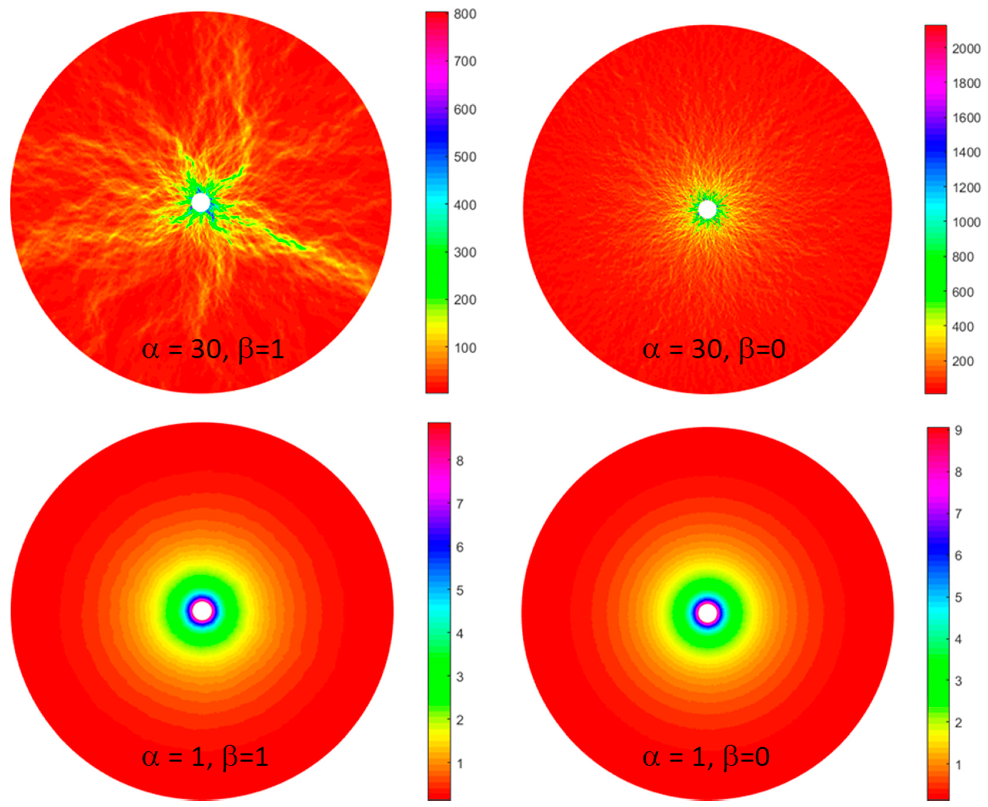
2.2. Flow From a Well: What Is at Stake

Figure 9 illustrates what is at stake in practical terms in the description of permeability as both lognormal and 1/k distributed. The figure depicts flow from a well to the sides of the computation domain, where the injected fluid is allowed to freely escape the system. The figure was generated by Matlab finite-element methods for different values of β and α in Equations (2) and (4). Uncorrelated (β = 0) and correlated (β = 1) porosity distributions are assigned to 10⁵ unstructured elements with the grid resolution increasing strongly toward the injection well. Corresponding permeability was derived from porosity assuming α = 1 or 30. The mean porosity is selected such that αϕ₀ ~3 to 4 in all panels. The method of flow computation is the same as is used to simulate the flow vectors shown in Figure 7.

If the permeability has little variation around its mean (small ${\sigma }_{\ln \kappa }$), the flow proceeds radially away from the well (lower two images) regardless of whether the ln permeability (and porosity) is spatially ordered as pink (β =1, 1/k) or white (β =1, random) noise. However, if the magnitude of permeability variation around its mean is of the order shown in Figure 2, Figure 3 and Figure 4, and the ln permeability is spatially ordered (1/k), flow from the well occurs through a spatially correlated dendritic or filamentary pattern (top left image). The flow does not have this pattern if the ln permeability distribution is uncorrelated (white noise), even if the permeability has a large spread from its mean (top right image). Both substantial permeability inhomogeneity and a pink noise spatial ln permeability distribution are required to produce the channelized/filamentary flow shown in the top left panel of Figure 9.

The earth’s crust meets both these criteria for channelized flow (permeability inhomogeneity and pink noise, scale invariant, spatial ln permeability distribution) as the following references in various areas attest: oil/gas (USEIA 2011), geothermal [30], mineral deposition [31,32,33,34,35,36] and trace elements [37,38,39,40]. The spatially heterogeneous, length-scale dependence of permeability is documented from lab-scale cm to reservoir-scale km [8,41,42,43,44,45]. The normal distributions, often assumed for modeling and analysis of flow in the earth’s crust, offer no formalism for dealing with the spatial variations (channeling) observed in the actual flow system (e.g., [21,22,46,47,48,49,50,51,52,53,54,55]).

3. Summary and Discussion

Flow measurements are difficult to make at even a few meters from a drill hole. However, we can infer the characteristics of flow far away from the wellbore from the observed variation in permeability about its mean and from the observed spatial distribution of permeability. Our analysis proceeds from the observations that (1) variations in crustal porosity and pore connections are invariably associated with variations in the logarithm of crustal permeability ($\delta \phi \propto \delta \ln \kappa$) and (2) the Fourier spectral power fluctuations in permeability magnitude (and all rock properties, micro-earthquakes, etc., associated with flow in fractures) scale inversely with spatial frequency (1/k).

Integrating the first observation produces an exponential relationship $\kappa \approx {\kappa }_0\exp \left(\alpha \left(\phi -{\phi }_0\right)\right)$, in which the variation in permeability magnitude relative to its mean is specified by a parameter $\alpha ={\sigma }_{\ln \kappa }/{\sigma }_{\phi }$. The permeability in the Earth’s crust has a substantial spread and the Earth’s crust is critically stressed which means that αϕ_ο = 3 to 4 and permeability has a 1/k (pink noise) spatial distribution. Consequently flow in the crust will become increasingly channelized as the distance of the flow increases.

The relationships described in this paper are physically fundamental. A connection condition explains why changes in porosity or the number of fractures in a volume are related to changes in log permeability magnitude. The pink noise spatial distribution of permeability is the distribution for which scale cannot be determined from observations. Geologists have long been aware that geological observations are scale invariant [56,57]. The parameter combination αϕ_ο = 3 to 4 defines the critical point of failure for the crust, for which this scale invariance will pertain.

Critical State Physics studies show that near the point of critical failure many parameters have a pink noise spatial distribution and that their magnitudes depend more on the proximity to critical failure than to other factors [18]. This greatly simplifies understanding crustal permeability. That fractures are closely involved in the critical state of the crust may not be surprising. Fluid-filled fractures are the weakest element in the crust. The crust may be in a critical state because, in this state, fluids can move, as required by compaction and tectonic deformation, through permeable pathways at all scales (millimeters to kilometers). Fluids may control crustal properties more than presently appreciated.

The framework described in this paper is also of great practical importance. Flow channelization poses a risk to many engineering and commercial pursuits. That flow channelization must be expected in the Earth’s crust as the distance of flow increases is thus significant. The fact that flow channels might be mapped by fracture seismic methods, as described by Sicking and Malin (2019) [1], means that, for the first time, the location of the major flow channels at a particular site can be determined and specified in models. The self-similar nature of permeability and the standard deviation of ln permeability from its mean allows the flow-field to be modelled in a statistically realistic way at finer scales. The combination of specific flow channel modeling with statistically realistic modeling of the finer details could produce more realistic and useful models of subsurface fluid flow for reservoir development and management, contaminant remediation, geothermal energy extraction, and many other purposes.

References

1. Sicking, C.; Malin, P. Fracture Seismic: Mapping Subsurface Connectivity. Geosciences 2019, 9, 508. [Google Scholar] [CrossRef] [Green Version]
2. Rutledge, J.T. Faulting Induced by Forced Fluid Injection and Fluid Flow Forced by Faulting: An Interpretation of Hydraulic-Fracture Microseismicity, Carthage Cotton Valley Gas Field, Texas. Bull. Seism. Soc. Am. 2004, 94, 1817–1830. [Google Scholar] [CrossRef]
3. Lacazette, A.; Vermilye, J.; Fereja, S.; Sicking, C. Ambient Fracture Imaging: A New Passive Seismic Method. In Proceedings of the Unconventional Resources Technology Conference, Denver, Colorado, 12–14 August 2013; pp. 2331–2340. [Google Scholar]
4. Leary, P.C. Deep borehole log evidence for fractal distribution of fractures in crystalline rock. Geophys. J. Int. 1991, 107, 615–628. [Google Scholar] [CrossRef] [Green Version]
5. Leary, P.C. Rock as a critical-point system and the inherent implausibility of reliable earthquake prediction. Geophys. J. Int. 1997, 131, 451–466. [Google Scholar] [CrossRef] [Green Version]
6. Leary, P.C. Fractures and physical heterogeneity in crustal rock. In Heterogeneity of the Crust and Upper Mantle – Nature, Scaling and Seismic Properties; Goff, J.A., Holliger, K., Eds.; Kluwer Academic/Plenum Publishers: New York, NY, USA, 2002; pp. 155–186. [Google Scholar]
7. Leary, P.C.; Al-Kindy, F. Power-law scaling of spatially correlated porosity and log(permeability) sequences from north-central North Sea Brae oilfield well core. Geophys. J. Int. 2002, 148, 426–442. [Google Scholar] [CrossRef] [Green Version]
8. Leary, P.; Malin, P.; Pogacnik, J. Computational EGS—Heat transport in 1/f-noise fractured media. In Proceedings of the 37th Stanford Geothermal Workshop, Stanford, CA, USA, 30 January–1 February 2012. [Google Scholar]
9. Leary, P.; Pogacnik, J.; Malin, P. Fractures ~ Porosity → Connectivity ~ Permeability → EGS Flow. In Proceedings of the Geothermal Resources Council 36th Annual Conference, Reno, NV, USA, 27 September 2012. [Google Scholar]
10. Leary, P.; Malin, P.; Saarno, T.; Heikkinen, P.; Diningrat, W. Coupling Crustal Seismicity to Crustal Permeability—Power-Law Spatial Correlation for EGS-Induced and Hydrothermal Seismicity. In Proceedings of the 44th Workshop on Geothermal Reservoir Engineering Stanford University, Stanford, CA, USA, 11–13 February 2019. [Google Scholar]
11. Barton, C.C. Fractal analysis of scaling and spatial clustering of fractures. In Fractals in the Earth Sciences; Barton, C.C., LaPointe, P.R., Eds.; Plenum Press: New York, NY, USA, 1995; pp. 141–178. [Google Scholar]
12. Leary, P.; Malin, P.; Niemi, R. Fluid Flow and Heat Transport Computation for Power-Law Scaling Poroperm Media. Geofluids 2017, 2017, 1–12. [Google Scholar] [CrossRef]
13. Leary, P.; Malin, P.; Saarno, T.; Kukkonen, I. αϕ ~ αϕcrit –Basement Rock EGS as Extension of Reservoir Rock Flow Processes. In Proceedings of the 43rd Workshop on Geothermal Reservoir Engineering, Stanford University, Stanford, CA, USA, 12–14 February 2018. [Google Scholar]
14. Nelson, P.H.; Kibler, J.E. A Catalog of Porosity and Permeability from Core Plugs in Siliciclastic Rocks; US Geological Survey: Reston, VA, USA, 2003. [Google Scholar]
15. Shockley, W. On the Statistics of Individual Variations of Productivity in Research Laboratories. Proc. IRE 1957, 45, 279–290. [Google Scholar] [CrossRef]
16. Binney, J.J.; Dowrick, N.J.; Fisher, A.J.; Newman, M.E.J. Theory of Critical Phenomena: An Introduction to the Renormalization Group; Clarendon Press: Oxford, UK, 1995; p. 464. [Google Scholar]
17. Stauffer, D.; Aharony, A. Introduction to Percolation Theory; Taylor & Francis: London, UK, 1994; p. 192. [Google Scholar]
18. Hunt, A.G.; Sahimi, M. Flow, Transport, and Reaction in Porous Media: Percolation Scaling, Critical-Path Analysis, and Effective Medium Approximation. Rev. Geophys. 2017, 55, 993–1078. [Google Scholar] [CrossRef]
19. Bak, P. How Nature Works: The Science of Self-Organized Criticality; Copernicus: Göttingen, 1996; p. 229. [Google Scholar]
20. Barton, C.C.; Camerlo, R.H.; Bailey, S.W. Bedrock geologic map of the Hubbard Brook experimental forest and maps of fractures and geology in roadcuts along interstate 93, Grafton County, New Hampshire, Sheet 1, Scale 1:12,000; Sheet 2, Scale 1:200: U.S. Geological Survey Miscellaneous Investigations Series Map I-2562. 1997. [Google Scholar]
21. Slatt, R.M.; Minken, J.; Van Dyke, S.K.; Pyles, D.R.; Witten, A.J.; Young, R.A. Scales of Heterogeneity of an Outcropping Leveed-channel Deep-water System, Cretaceous Dad Sandstone Member, Lewis Shale, Wyoming, USA. In Atlas of Deep-Water Outcrops; Nilsen, T.H., Shew, R.D., Steffens, G.S., Stud¬lick, J.R.J., Eds.; American Association of Petroleum Geologists: Tulsa, OA, USA, 2006. [Google Scholar]
22. Slatt, R.M.; Eslinger, E.; Van Dyke, S. Acoustic and petrophysical heterogeneities in a clastic deepwater depositional system: implications for up scaling from bed to seismic scales. Geophysics 2009, 74, 35–50. [Google Scholar] [CrossRef]
23. Malamud, B.D.; Turcotte, D.L. Self-afine time series: I. Generation and Analysis. Adv. Geophys. 1999, 40, 1–90. [Google Scholar]
24. Hubbert, M.K. Darcy’s law and the field equations of the flow of underground fluids. Int. Assoc. Sci. Hydrol. Bull. 1957, 2, 23–59. [Google Scholar] [CrossRef] [Green Version]
25. Warren, J.E.; Root, P.J. The behavior of naturally fractured reservoirs. Soc. Pet. Eng. J. 1963, 3, 245–255. [Google Scholar] [CrossRef] [Green Version]
26. Bear, J. Dynamics of Fluids in Porous Media; American Elsevier: New York, NY, USA, 1972. [Google Scholar]
27. Leary, P.C.; Malin, P.E.; Saarno, T. A physical basis for the gutenberg-richter fractal scaling. In Proceedings of the 45rd Workshop on Geothermal Reservoir Engineering, Stanford University, Stanford, CA, USA, 10–12 February 2020. [Google Scholar]
28. Kwiatek, G.; Saarno, T.; Ader, T.; Bluemle, F.; Bohnhoff, M.; Chendorain, M.; Dresen, G.; Heikkinen, P.; Kukkonen, I.; Leary, P.; et al. Controlling fluid-induced seismicity during a 6.1-km-deep geothermal stimulation in Finland. Sci. Adv. 2009, 5, eaav7224. [Google Scholar] [CrossRef] [PubMed] [Green Version]
29. Lacazette, A.; Geiser, P. Comment on Davies et al., 2012–Hydraulic fractures: How far can they go? Mar. Pet. Geol. 2013, 43, 516–518. [Google Scholar] [CrossRef]
30. Grant, M.A. Optimization of drilling acceptance criteria. Geothermics 2009, 38, 247–253. [Google Scholar] [CrossRef]
31. De Wijs, H.J. Statistics of ore distribution. Part I: frequency distribution of assay values. J. R. Neth. Geol. Min. Soc. New Ser. 1951, 13, 365–375. [Google Scholar]
32. De Wijs, H.J. Statistics of ore distribution Part II: theory of binomial distribution applied to sampling and engineering problems. J. R. Neth. Geol. Min. Soc. New Ser. 1953, 15, 125-24. [Google Scholar]
33. Koch, G.S.; Link, R.F. The coefficient of variation; a guide to the sampling of ore deposits. Econ. Geol. 1971, 66, 293–301. [Google Scholar] [CrossRef]
34. Clark, I.; Garnett, R.H.T. Identification of multiple mineralization phases by statistical methods. Trans. Inst. Min. Metall. 1974, 83, A43. [Google Scholar]
35. Link, R.F.; Koch, G.S., Jr. Some consequences of applying lognormal theory to pseudolognormal distributions. Math. Geol. 1975, 7, 117–128. [Google Scholar] [CrossRef]
36. Gerst, M.D. Revisiting the Cumulative Grade-Tonnage Relationship for Major Copper Ore Types. Econ. Geol. 2008, 103, 615–628. [Google Scholar] [CrossRef]
37. Ahrens, L.H. The lognormal distribution of the elements, I. Geochim. Cosmochim Acta 1954, 5, 49–73. [Google Scholar] [CrossRef]
38. Ahrens, L.H. The lognormal-type distribution of the elements, II. Geochim. Cosmochim. Acta 1954, 6, 121–131. [Google Scholar] [CrossRef]
39. Ahrens, L.H. Lognormal distributions, III. Geochim. Cosmochim. Acta 1957, 11, 205–212. [Google Scholar] [CrossRef]
40. Ahrens, L.H. Lognormal-type distributions in igneous rocks, IV. Geochim. Cosmochim. Acta 1963, 27, 333–343. [Google Scholar] [CrossRef]
41. Brace, W.F. Permeability of crystalline and argillaceous rocks. Int. J. Rock Mech. Miner. Sci. Geomech. Abstr. 1980, 17, 241–251. [Google Scholar] [CrossRef]
42. Clauser, C. Scale Effects of Permeability and Thermal Methods as Constraints for Regio-nal-Scale Averages. In Heat and Mass Transfer in Porous Media; Quintard, M., Todorovic, M., Eds.; Elsevier: Amsterdam, The Netherlands, 1992; pp. 446–454. [Google Scholar]
43. Neuman, S.P. Generalized scaling of permeabilities: Validation and effect of support scale. Geophys. Res. Lett. 1994, 21, 349–352. [Google Scholar] [CrossRef] [Green Version]
44. Neuman, S.P. On advective dispersion in fractal velocity and permeability fields. Water Resour. Res. 1995, 31, 1455–1460. [Google Scholar] [CrossRef]
45. Schulze-Makuck, D.; Cherhauer, D.S. Relation of hydraulic conductivity and dispersivity to scale of measurement in a carbonate aquifer. In Models for Assessing and Monitoring Groundwater Quality; Wagner, B.J., Illangasekare, T.H., Jensen, K.H., Eds.; Indigenous Allied Health Australia: Deakin, Australia, 1995. [Google Scholar]
46. Archie, G.E. Introduction to Petrophysics of Reservoir Rocks. AAPG Bull. 1950, 34, 943–961. [Google Scholar]
47. Biot, M.A. General theory of three-dimensional consolidation. J. Appl. Phys. 1941, 12, 155–164. [Google Scholar] [CrossRef]
48. Carman, P.C. Fluid flow through granular beds. Trans. Inst. Chem. Engrs. 1937, 15, 150–166. [Google Scholar] [CrossRef]
49. Amyx, J.W.; Bass, D.M.; Whiting, R.L. Petroleum reservoir engineering: Physical properties; McGraw-Hill: New Year, NY, USA, 1960; p. 610. [Google Scholar]
50. Timur, A. An investigation of permeability, porosity, and residual water saturation relationships. In Proceedings of the SPWLA 9th Annual Logging Symposium, New Orleans, LA, USA, 23–26 June 1968. [Google Scholar]
51. Hearst, J.R.; Nelson, P. Well Logging for Physical Properties; McGraw-Hill: New York, NY, USA, 1985; p. 571. [Google Scholar]
52. Nelson, P.H. Permeability-porosity relationships in sedimentary rocks. Soc. Petrophys. Well-Log Anal. 1994, 35, 38–62. [Google Scholar]
53. Jensen, J.L.; Hinkley, D.V.; Lake, L.W. A Statistical Study of Reservoir Permeability: Distributions, Correlations, and Averages. SPE Form. Evaluation 1987, 2, 461–468. [Google Scholar] [CrossRef]
54. Ingebritsen, S.; Sanford, W.; Neuzil, W. Groundwater in Geological Processes; Cambridge University Press: Cambridge, UK, 1999; p. 536. [Google Scholar]
55. Mavko, G.; Mukerji, T.; Dvorkin, J. The Rock Physics Handbook: Tools for Seismic Analysis of Porous Medial; Cambridge University Press: Cambridge, UK, 1998; p. 2009. [Google Scholar]
56. Barton, C.C.; La Pointe, P.R. Fractals in the Earth Sciences; Springer (Plenum Press): New York, NY, USA, 1995. [Google Scholar]
57. Barton, C.C.; La Pointe, P.R. Fractals in Petroleum Geology and Earth Processes; Springer (Plenum Press): New York, NY, USA, 1995. [Google Scholar]
Figure 1. (Top) A horizontal map slice of the above background Fracture Seismic (FS) intensity (red high, blue low), activated during the third stage of a fracture stimulation treatment. (Bottom) The above-background FS intensity (red high, blue low) backbone of the same horizontal map slice in the FS intensity cloud for hydrofracturing Stages 3–5. Point A is the wellhead of a horizontal well with a trajectory indicted by the black line. Point B shows the location of a vertical well with pressure and chemical tracer monitors. Both pressure and tracer communicated between Well B and Well A, where the FS skeleton connects the wells over a distance of 600 m. Figure is from Lacazette et al (2013) [3].
Geosciences 10 00050 g001
Figure 2. Porosity and permeability measurements on four sub-vertical North Sea gas field well cores. (Left panel) Histograms of porosity values are plotted as number of values in 1% wide bins versus percent porosity. Both log permeability and permeability data are plotted as the number of values in a bin versus millidarcies. The histograms suggest that the porosity has a normal, and the permeability a lognormal, distribution. (Two right panels) Porosity (blue) and natural ln permeability (red) data are plotted as functions of sample number. The porosity and permeability data are normalized to zero mean and unit variance.
Geosciences 10 00050 g002
Figure 3. Porosity (ϕ, blue ) and natural log permeability (ln κ, red) magnitudes in sub-vertical well cores from the North Sea (top), Germany (middle), and South Australia (bottom). Porosity and ln permeability are plotted against sample depth. Both are normalized to zero mean and unit variance. The number of measurements is shown on the plots. In the histograms, the porosity values are plotted as the number of values in 1% wide bins versus percent porosity. Both ln permeability and permeability data are plotted as the number of values in bins versus millidarcies (mD).
Geosciences 10 00050 g003
Figure 4. (Top) Porosity (ϕ, blue) and ln permeability (ln κ, red) measurements from a horizontal well from North Sea clastic oil fields, plotted with zero-mean and unit variance. (Bottom) Histograms of the number of measurements in bins of equal porosity, ln κ, or κ.
Geosciences 10 00050 g004
Figure 5. Time-series analysis well-log properties related to flow in fractures. From top left to bottom right, these properties are: acoustic velocity, gamma ray intensity, potassium abundance, potassium-thorium abundance, neutron porosity, thorium abundance, uranium abundance, mass density correlation, and mass density. In all these panels, the spectral density S(k) (y-axis) falls off with frequency as ~1/k, where k is spatial scale-length measured in number of cycles per km (x-axis). Data are from a sand-shale well-log provided to us courtesy of R Slatt [21,22]. The power-scaling exponent is shown in the red box at the upper right of each plot.
Geosciences 10 00050 g005
Figure 6. (a): Spatially uncorrelated and (b) correlated hypothetical porosity models. (Top): Map views of porosity variation indicated by color. (Middle) Representative synthetic porosity well-logs in an arbitrary direction through the porosity map view images above. The ordinate is distance and the abscissa is the magnitude of porosity. (Bottom): Power spectrum of synthetic well-log porosity, plotting the square of harmonic amplitude (ordinate) against spatial frequency (cycles per km) on abscissa. Numbers are the power exponents (-β ) of the power spectra (see Equation (4)). They confirm that the left map distribution is spatially uncorrelated white noise (β ~ 0) and the right map distribution is spatially correlated 1/k pink noise (β ~ 1).
Geosciences 10 00050 g006
Figure 7. a. The flow field, computed for a medium with a permeability that varies by ±2 natural log units (see Figure 2, Figure 3 and Figure 4 well-core data) and has a 1/k spatial distribution of ln κ, shows dramatic channeling between the high- and low-pressure boundaries. b. Distribution of natural log-well log-flow velocity, ln (V), where V is in arbitrary units
Geosciences 10 00050 g007
Figure 8. (Left) Normalized length distributions of linear fracture seismic intensity segments from four different reservoirs: (Clockwise) Marcellus, Utica, East Asia, Wayland. Linear backbone segments can be seen in the fracture seismic map slice in the bottom image in Figure 1. (Right) Normalized histograms of seismic fracture emission intensity recorded shale reservoir fracks, above. Data are from Lacazette et al. (2013) [29].
Geosciences 10 00050 g008
Figure 9. Flow calculated from a central well to free-flow boundaries where it escapes the system for different values of α in Equations (2) and (3) and β in Equation (4). Color indicates the relative magnitude of the fluid velocity (red low, purple high). Flow channeling (upper left panel) requires that both a large spread in ln κ from its mean (e.g., α =30) and a distribution in permeability that is pink (β = 1). The variation in the magnitude of permeability from its mean can be large, but cannot produce channel flow if its spatial variation is that of spatially uncorrelated white noise (top right panel). The permeability distribution can be 1/k (pink noise) but cannot produce channel flow unless the variation in ln permeability is also large (bottom left panel). When the permeability distribution is white and the spread in ln permeability small, the flow from the well is of course uniform (bottom right panel).
Geosciences 10 00050 g009