The 2017 Rigopiano Avalanche—Dynamics Inferred from Field Observations


Abstract
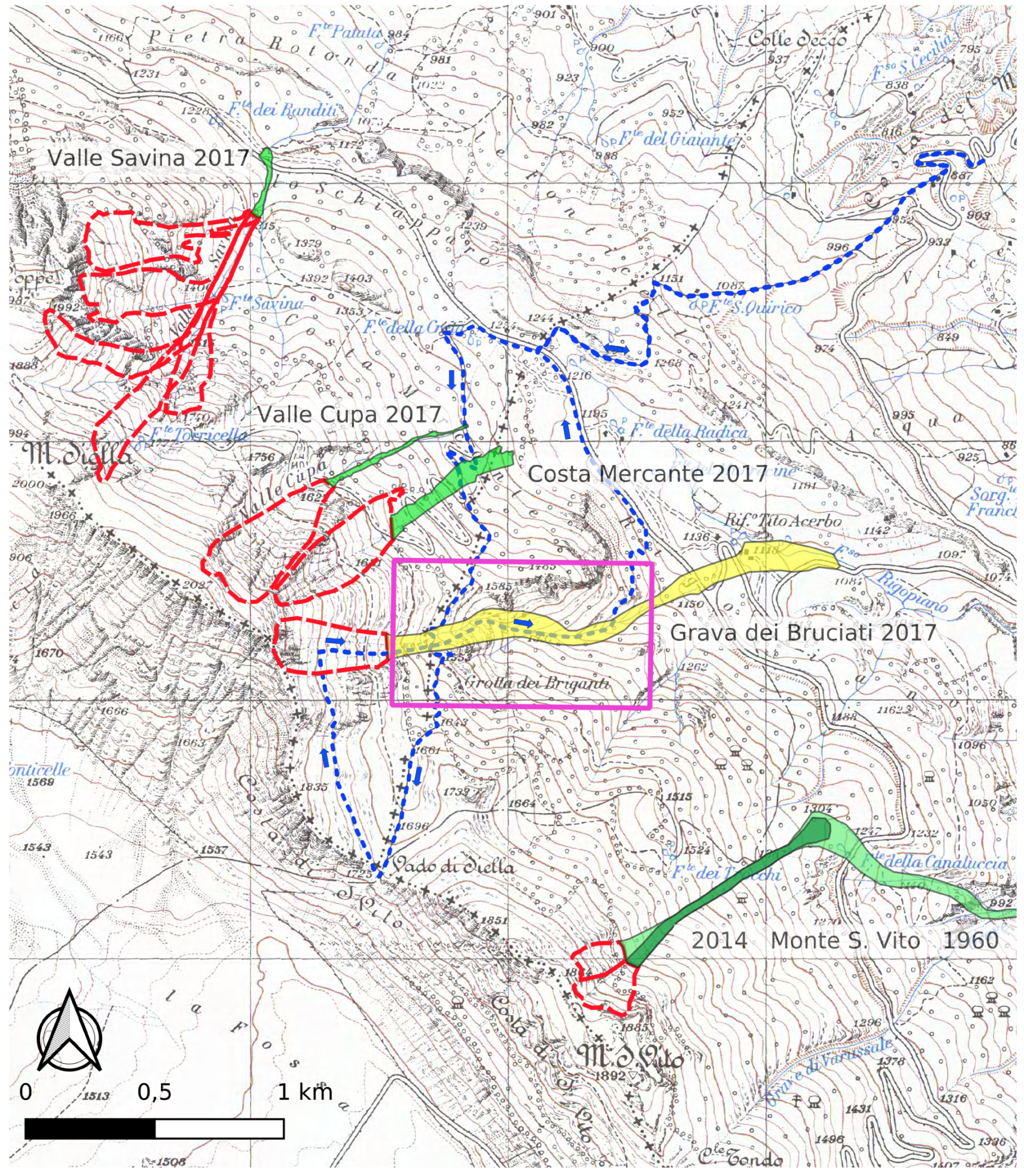
1. Introduction
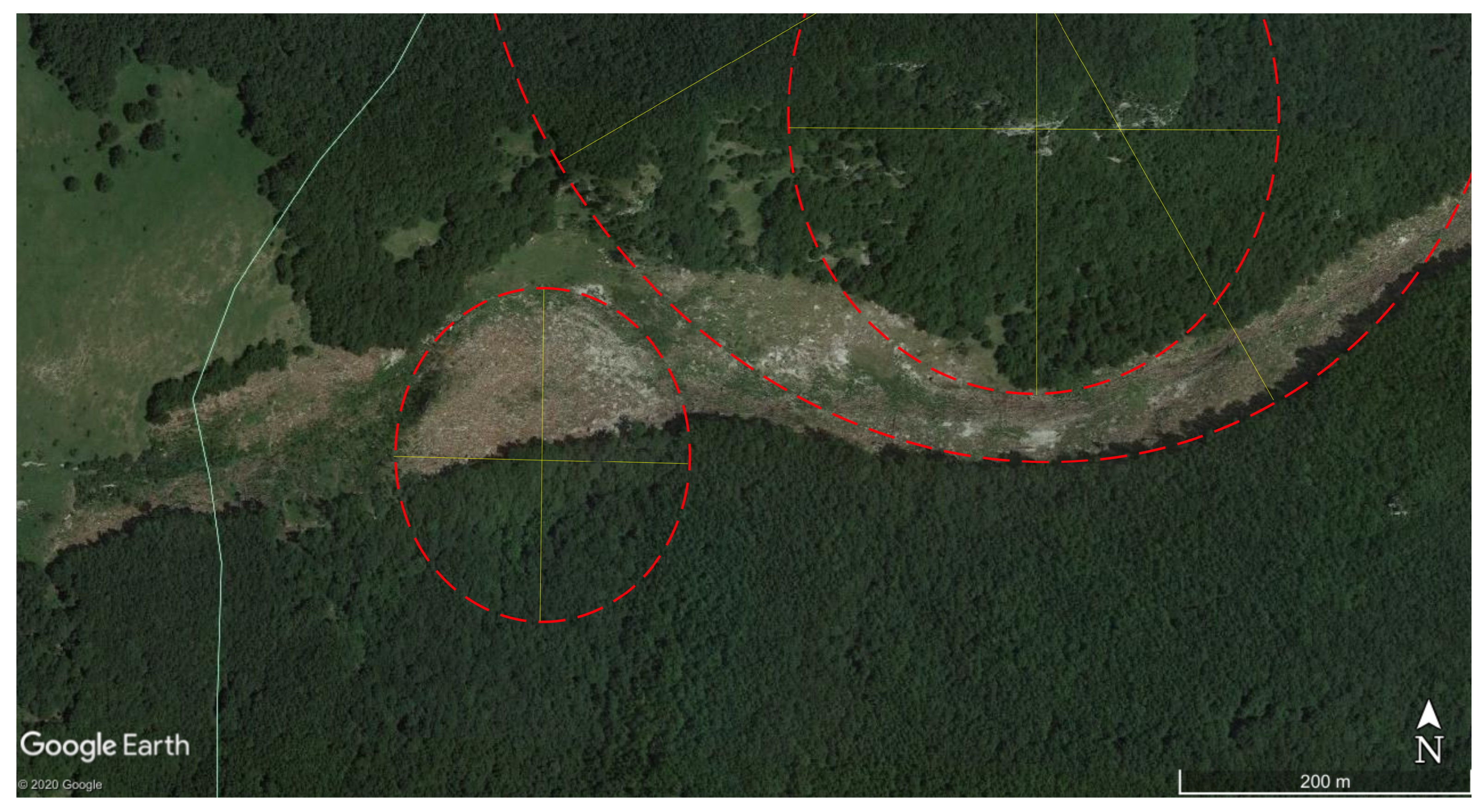
2. Comparison with a Topographic-Statistical Run-Out Model
3. Velocity Estimates
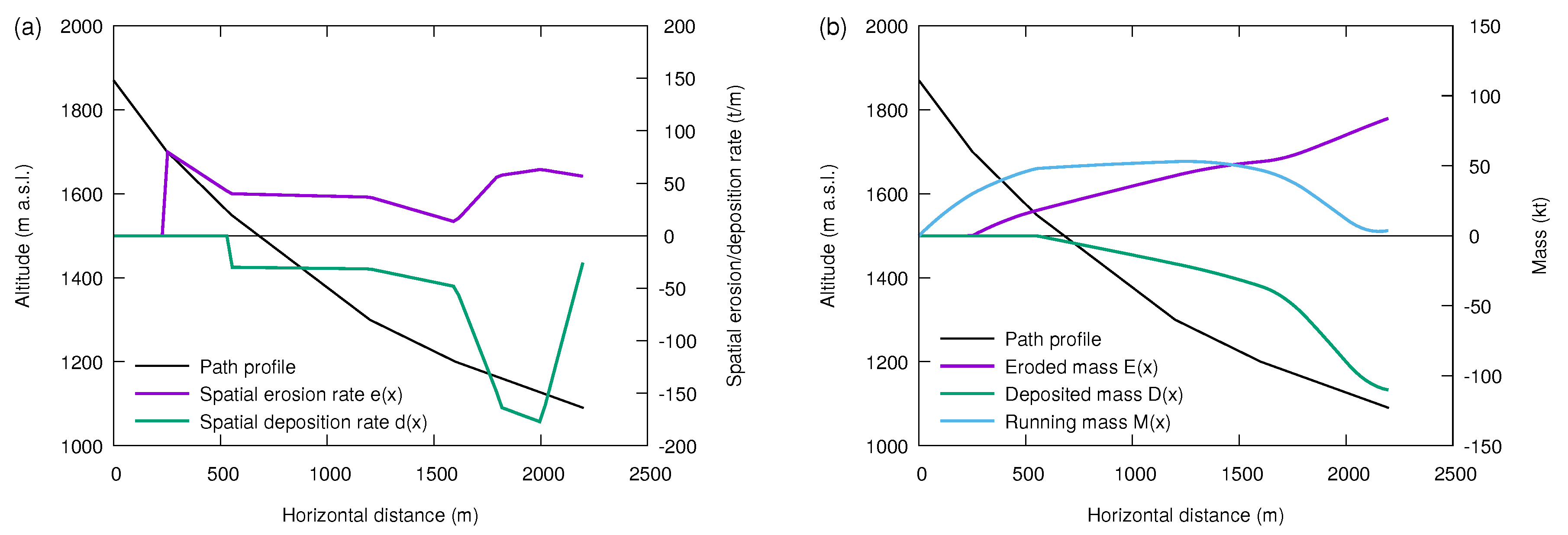
4. Estimate of the Mass Balance
- Along most of the track and probably also in the run-out zone, most of the snow cover was eroded, including the old snow.
- There is no observational information about erosion and deposition in the upper track above 1550 m a.s.l., but based on experience from other avalanche paths (Monte Pizzac, Vallée de la Sionne, Ryggfonn), it is likely that while the net entrainment rate probably was almost equal to the erosion rate so that increased rapidly in that path segment.
- In the middle and lower track, deposition appears to have equaled or exceeded erosion. The likely causes are the diminishing slope angle and increased dissipation due to still intact or already uprooted trees.
- The deposited mass in the run-out area below 1200 m a.s.l. is much larger than the mass of the snow cover before the avalanche. It is likely that the mass increase in the run-out zone also exceeds the release mass. This would mean that and that the running mass, , of the avalanche increased, at least in the steeper parts of the path down to perhaps 1400 or 1300 m a.s.l.
- Detailed measurements at Vallée de la Sionne as well as dynamical considerations [19] indicate that deposition occurs only in the tail of an avalanche, except right before it stops. This suggests that much of the fully entrained snow—possibly stemming from the upper layers of the snow cover—traveled over a large distance, whereas older snow from near the ground was dragged along a relatively short distance and subsequently deposited when the tail of the avalanche passed over it.
- On the one hand, substantial masses of tree debris were deposited near the distal end of the avalanche, where there had been no forest. This implies that some trees were dragged at least 200–300 m by the avalanche. On the other hand, uprooted or broken trees were found a short distance below the point where the avalanche entered the forest. This suggests that the tree destruction rate (the mass of trees per unit area that were broken and/or uprooted) in a dense forest exceeds the debris deposition rate at least in the steeper reaches of the path and that it also exceeds the debris entrainment rate along the forested part of the path.
5. Observational Limits on Impact Pressure
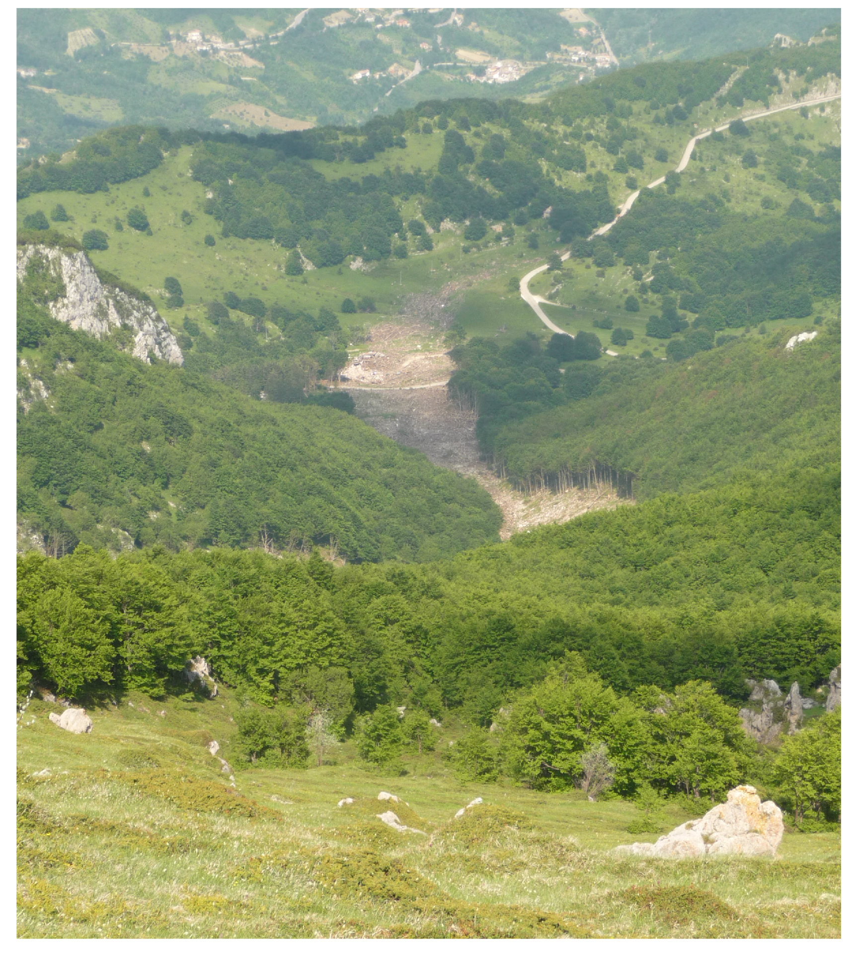
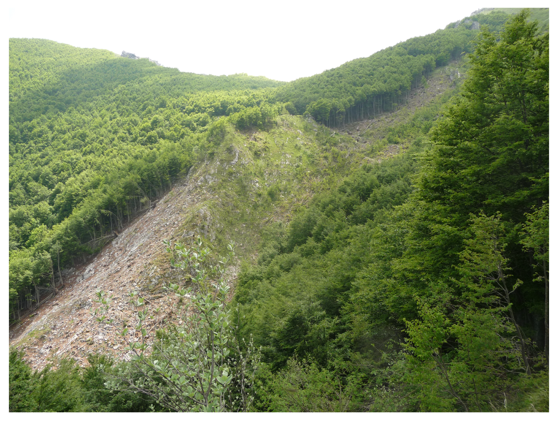
5.1. Limits Inferred From Forest Destruction
- Between 1550 and 1450 m a.s.l., we assume m, m s, W = 80 m, m, , and . This leads to GW.
- Between 1400 and 1200 m a.s.l., we set , m, m, , m and m s. From this, .
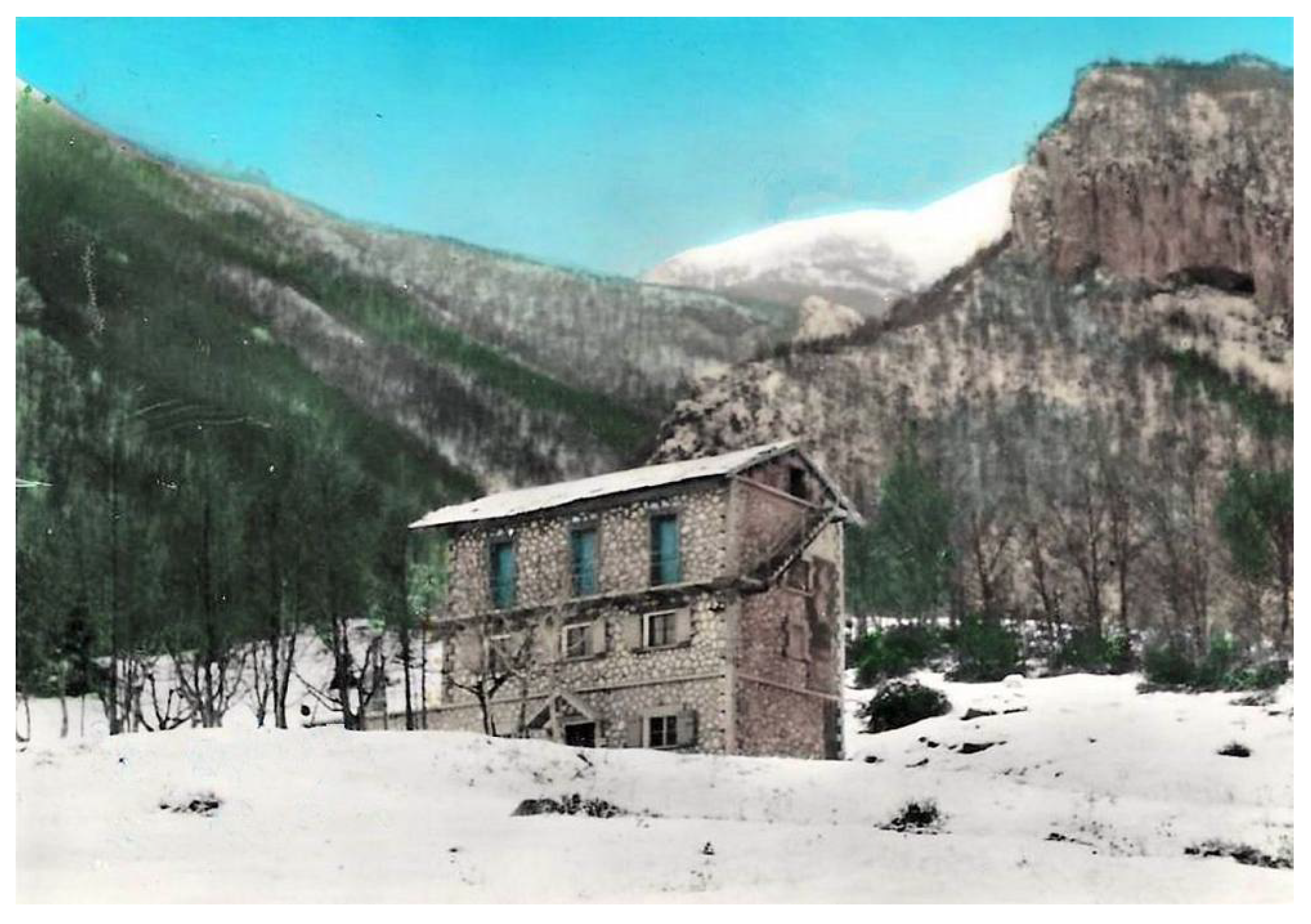
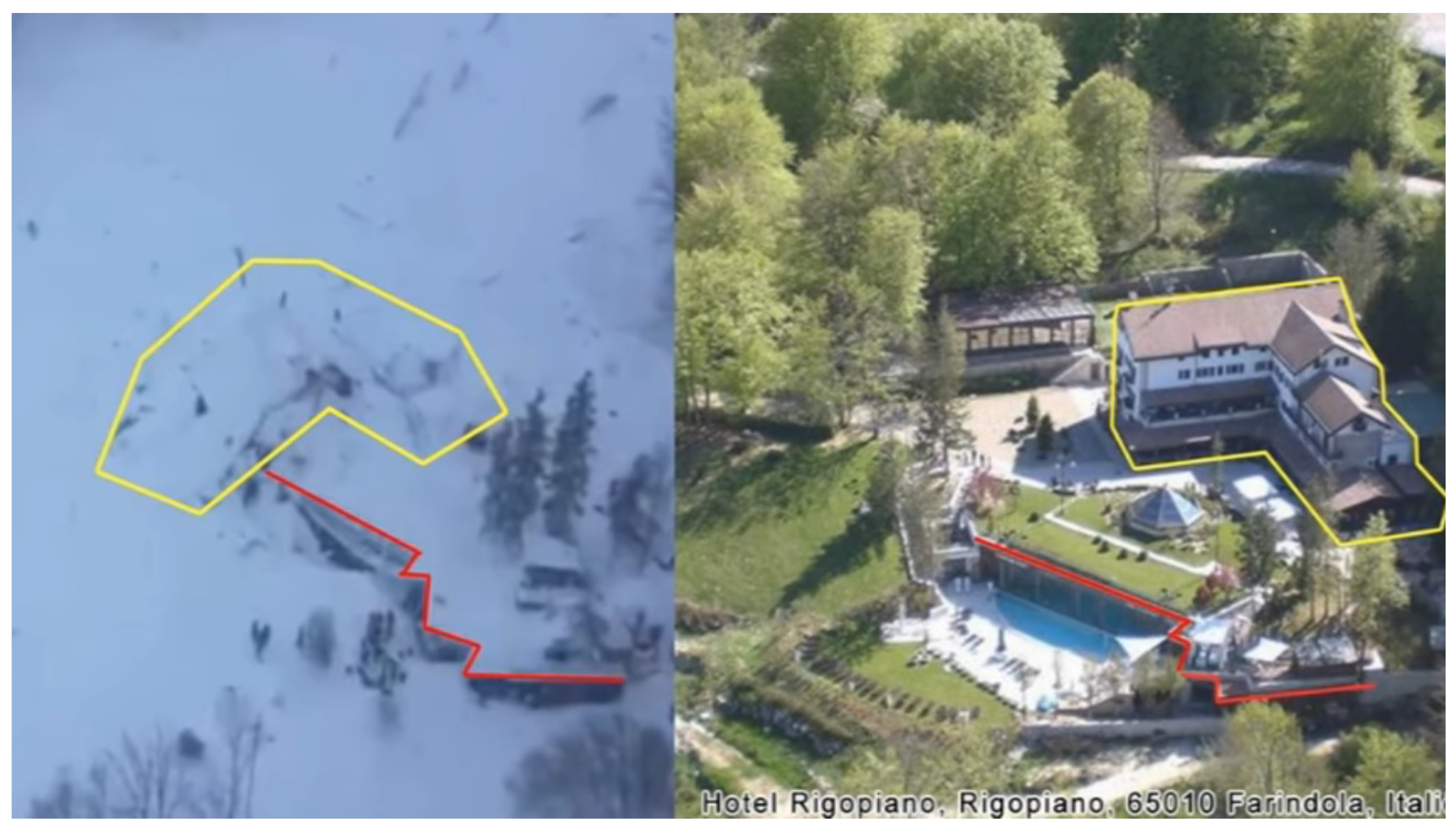
5.2. Limits from Damage to Hotel Rigopiano
6. On the Vulnerability of Buildings and Persons Hit by Snow Avalanches
- The main building can probably be classified as a large multi-story masonry building, whereas the newer spa complex was a one- or two-story reinforced-concrete construction. Neither of them was specifically dimensioned for avalanche impact. Note that these classifications need to be confirmed.
- The impact pressure of the avalanche can only be inferred from numerical simulations, which are fraught with large uncertainties because the initial conditions are poorly known and most models do not explicitly consider fluidization or the formation of a powder snow cloud.
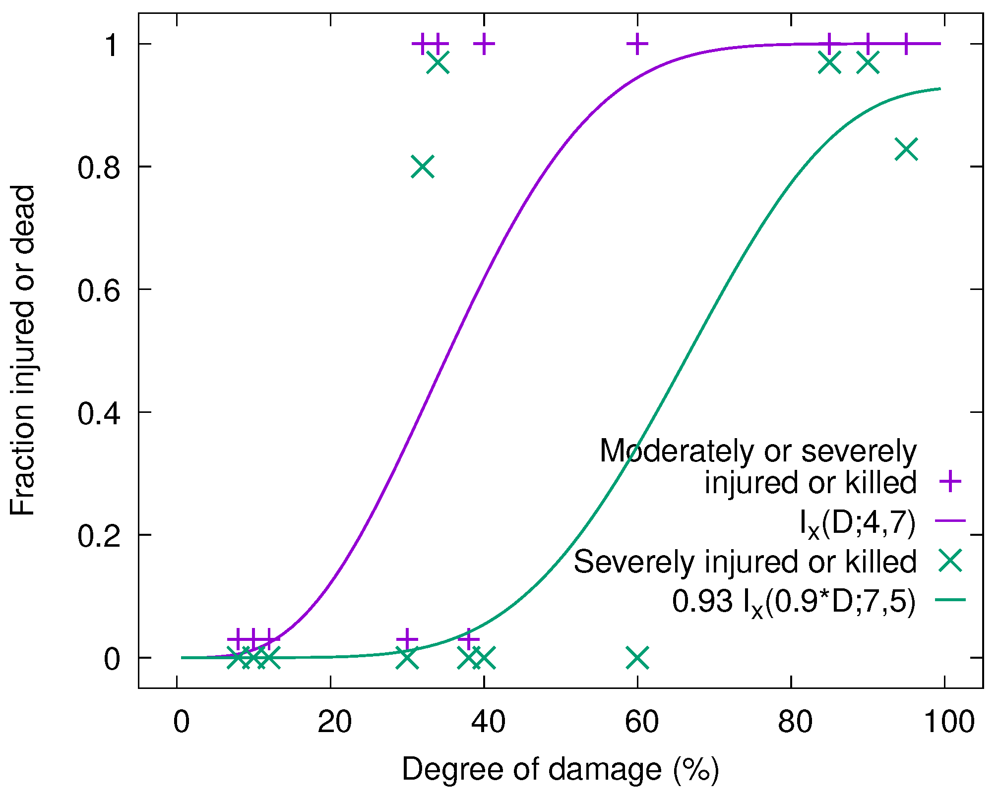
- The damage to the main building was in Category 5, .
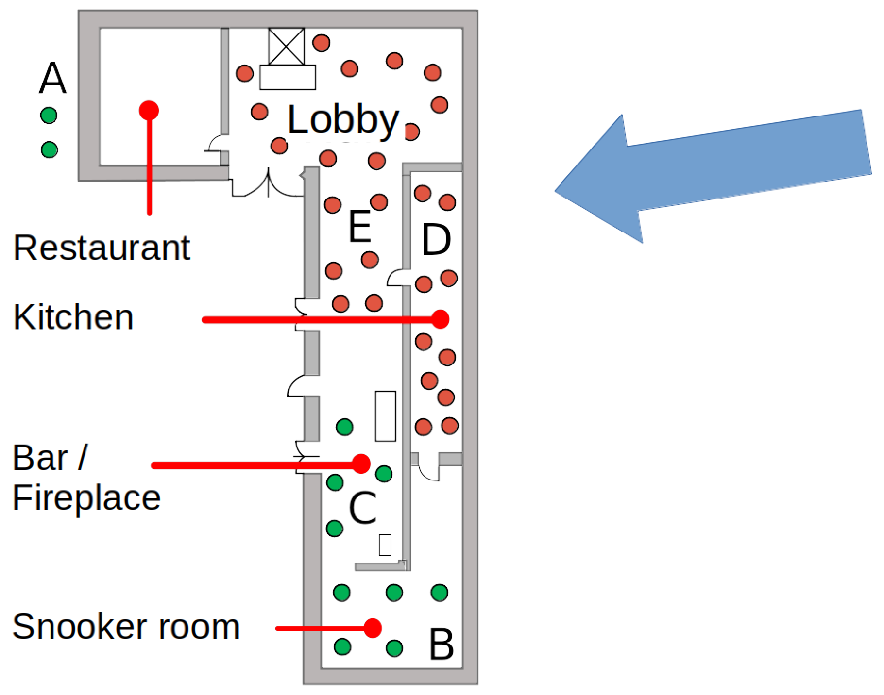
- Images in the media suggest that the spa complex collapsed only partially. Snow entered the building in large quantities and blocked the way for the children in the gaming room, but left them with enough space and air for surviving over an extended period. This points to damage in Category 3 and .
- There were a total of 38 persons inside the hotel complex, while two persons were in the parking lot outside the devastated area and were unharmed.
- Several children were playing in a room near the spa area, which was less exposed to the avalanche. The degree of damage was presumably in Category 3, i.e., between 0.4 and 0.7, as it took up to four days to rescue some of the children.
- Five of the adults were found alive. In at least two cases, the degree of damage seems to be in Category 4, yet the persons were only lightly injured.
- The death toll was 29 adults who were gathered in the hotel lobby at the time the avalanche struck. As the entire four-story main building was displaced some 10 m and completely collapsed, one can assume the degree of damage to be in Category 5.
- The data for damage in Categories 4 and 5 appear consistent between the Longyearbyen and Rigopiano events. Somewhat surprisingly, six persons out of 35 survived building damage of degree 5 in Rigopiano, despite the long time it took to find and free them.
- Within the statistical uncertainty, the data from the Rigopiano game room is also consistent with the findings from Longyearbyen, even though the three children in Rigopiano may have survived essentially unscathed in a quite severely damaged room. The degree of damage should, however, be reassessed once more detailed information is released.
7. Conclusions
- Among the four avalanches that occurred in the vicinity of Rigopiano on or around 18 January 2017, the avalanche that destroyed the hotel had a much longer run-out than the others relative to the prediction of the - model. The reasons for this remain uncertain.
- The estimated front speeds in the range of 35 to 60 m s have a wide margin of uncertainty, but the most likely values in the range of 40 to 45 m s are of the same order as observations, measurements and numerical simulations of avalanches of similar size. The slow-moving, dense parts of the avalanche appear to have moved at about half the speed of the front. This agrees with observations and analyses in small-to-medium size avalanche paths in the Swiss Alps [16].
- Estimates of the mass balance are also fraught with large uncertainties, but a consistent picture emerges. It is probable that a large part of the snow cover was eroded, but much of this mass was only dragged along for some distance without becoming properly entrained into the flow. Tree debris contributed much to the mass growth of the avalanche.
- The observed damage patterns are consistent with the pressures derived from the velocity estimates, both with respect to the destroyed forest and the obliterated and displaced hotel. Breaking or uprooting of the forest was not a dominant factor in the energy balance of the entire avalanche, but must have had a significant braking effect on the fluidized flow in the forest destruction zone.
- When expressed as a function of the degree of building damage, the lethality curve resulting from the Rigopiano event is consistent with the one found in the 2015 Longyearbyen avalanche within the large uncertainties due to the small statistical base. This supports the usefulness of the degree of damage as the proper variable for obtaining a universal relation that does not depend on the building type.
Funding
Acknowledgments
Conflicts of Interest
Appendix A. Derivation of Flow Velocity from Run-Up
Appendix B. Derivation of Flow Velocity from Super-Elevation
Appendix B.1. Characterization of the Topography
Appendix B.2. Time Dependence
Appendix B.3. Can Inertial Effects Be Neglected?

Appendix B.4. McClung’s Model for Super-Elevation in Granular Avalanches
Appendix B.5. Alternative Treatment of Granular Effects
Appendix B.6. Remarks on the Pudasaini–Jaboyedoff Super-Elevation Model
Appendix C. Forces, Moments and Energetics of Tree Breaking and Uprooting
Appendix D. Estimate of the Strength of Hotel Rigopiano against Avalanche Impact
References
- Issler, D. Field Survey of the 2017 Rigopiano Avalanche; NGI Technical Note 20170131-02-TN; Norwegian Geotechnical Institute: Oslo, Norway, 2018; Available online: https://www.ngi.no/download/file/14511 (accessed on 8 April 2020).
- Hotel Rigopiano, l’esposto del Forum H2O: “In queste foto la prova di valanghe precedenti”. 2017. Available online: https://www.repubblica.it/cronaca/2017/01/26/foto/rigopiano_forum_h2o-156964271 (accessed on 8 April 2020).
- Iannetti, P. Oggetto: Commissione Valanghe (L.R. n.47 del 18.06.92). Letter to the Mayor of Farindola. 1999. Available online: http://www.repubblica.it/static/infografica/cronaca/rigopiano/Relazione-Comune-Farindola-001.pdf (accessed on 10 November 2018).
- Chiambretti, I.; Chiaia, B.; Frigo, B.; Marello, S.; Maggioni, M.; Fantucci, R.; Bernabei, M. The 18th January 2017 Rigopiano avalanche disaster in Italy—Analysis of the applied forensic field investigation techniques. In Proceedings of the International Snow Science Workshop, Innsbruck, Austria, 7–12 October 2018; pp. 1208–1212. [Google Scholar]
- Chiambretti, I.; Sofia, S. Winter 2016–2017 snowfall and avalanche energency management in Italy (central Appennines)—A review. In Proceedings of the International Snow Science Workshop, Innsbruck, Austria, 7–12 October 2018; pp. 1445–1449. [Google Scholar]
- Tedim, F.; Leone, V. The deadly avalanche of Rigopiano (Italy): Evidences of a constructed local disaster. In The Overarching Issues of the European Space—Preparing the New Decade for Key Socio-economic and Environmental Challenges; Remoalda, P., Ed.; Faculdade de Letras da Universidade do Porto: Porto, Portugal, 2018; pp. 408–424. [Google Scholar]
- Frigo, B.; Chiaia, B.; Chiambretti, I.; Bartelt, P.; Maggioni, M.; Freppaz, M. The January 18th 2017 Rigopiano disaster in Italy—Analysis of the avalanche dynamics. In Proceedings of the International Snow Science Workshop, Innsbruck, Austria, 7–12 October 2018; pp. 6–10. [Google Scholar]
- Fischer, J.-T. BFW, Innsbruck, Austria. Personal communication to D. Issler, 2017. [Google Scholar]
- Bakkehøi, S.; Domaas, U.; Lied, K. Calculation of snow avalanche runout distance. Ann. Glaciol. 1983, 4, 24–29. [Google Scholar] [CrossRef]
- Issler, D.; Jónsson, Á.; Gauer, P.; Domaas, U. Vulnerability of houses and persons under avalanche impact—The avalanche at Longyearbyen on 2015-12-19. In Proceedings of the International Snow Science Workshop ISSW 2016, Breckenridge, CO, USA, 3–7 October 2016; pp. 371–378. [Google Scholar]
- Valanga di Rigopiano. 2017. Available online: https://it.wikipedia.org/wiki/Valanga_di_Rigopiano (accessed on 2 November 2020). (In Italian).
- Pudasaini, S.P.; Jaboyedoff, M. A general analytical model for superelevation in landslide. Landslides 2020, 17, 1377–1392. [Google Scholar] [CrossRef]
- Tarquini, S.; Isola, I.; Favalli, M.; Battistini, A. TINITALY, a Digital Elevation Model of Italy with a 10 m-Cell Size (Version 1.0). Data Set Prepared by Istituto Nazionale di Geofisica e Vulcanologia (INGV). 2007. Available online: http://tinitaly.pi.ingv.it/ (accessed on 22 October 2020). [CrossRef]
- Gauer, P. Considerations on scaling behavior in avalanche flow along cycloidal and parabolic tracks. Cold Regions Sci. Technol. 2018, 151, 34–46. [Google Scholar] [CrossRef]
- Smith, D.J.; McCarthy, D.P.; Luckman, B.H. Snow-avalanche impact pools in the Canadian Rocky Mountains. Arct. Alp. Res. 1994, 26, 116–127. [Google Scholar] [CrossRef]
- Issler, D.; Errera, A.; Priano, S.; Gubler, H.; Teufen, B.; Krummenacher, B. Inferences on flow mechanisms from snow avalanche deposits. Ann. Glaciol. 2008, 49, 187–192. [Google Scholar] [CrossRef]
- Issler, D.; Gauer, P.; Schaer, M.; Keller, S. Supplementary Materials: Field observations of three mixed snow avalanches. Geosciences 2020, 10, 2. [Google Scholar] [CrossRef]
- Sovilla, B.; Sommavilla, F.; Tomaselli, A. Measurements of mass balance in dense snow avalanche events. Ann. Glaciol. 2001, 32, 230–236. [Google Scholar] [CrossRef]
- Rauter, M.; Köhler, A. Constraints on entrainment and deposition models in avalanche simulations from high-resolution radar data. Geosciences 2020, 10, 9. [Google Scholar] [CrossRef]
- Sovilla, B. Field Experiments and Numerical Modelling of Mass Entrainment and Deposition Processes in Snow Avalanches. Ph.D. Thesis, ETH Zürich, Zürich, Switzerland, 2004. [Google Scholar] [CrossRef]
- Gauer, P.; Issler, D. Possible erosion mechanisms in snow avalanches. Ann. Glaciol. 2004, 38, 384–392. [Google Scholar] [CrossRef]
- Mattheck, C.; Bethge, K.; Kappel, R.; Mueller, P.; Tesari, I. Failure modes for trees and related criteria. In ‘Wind Effects on Trees’ Proceedings of the International Conference; Ruck, B., Kottmeier, C., Mattheck, C., Quine, C., Wilhelm, G., Eds.; Laboratory of Building and Environmental Aerodynamics, Institute for Hydromechanics, University of Karlsruhe: Karlsruhe, Germany, 2003; p. P9/1. ISBN 3-00-011922-1. [Google Scholar]
- Ribeiro, G.H.P.M.; Chambers, J.Q.; Peterson, C.J.; Trumbore, S.E.; Magnabosco Marra, D.; Wirth, C.; Cannon, J.B.; Négron-Juárez, R.I.; Lima, A.J.N.; de Paula, E.V.C.M.; et al. Mechanical vulnerability and resistance to snapping and uprooting for Central Amazon tree species. For. Ecol. Mgmt. 2016, 380, 1–10. [Google Scholar] [CrossRef]
- Gauer, P.; Lied, K.; Kristensen, K. On avalanche measurements at the Norwegian full-scale test-site Ryggfonn. Cold Reg. Sci. Technol. 2008, 51, 138–155. [Google Scholar] [CrossRef]
- Bartelt, P.; Christen, M.; Bühler, Y.; Caviezel, A.; Buser, O. Snow entrainment: Avalanche interaction with an erodible substrate. In Proceedings of the International Snow Science Workshop, Innsbruck, Austria, 7–12 October 2018; pp. 716–720. [Google Scholar]
- Favillier, A.; Guillet, S.; Morel, P.; Corona, C.; Lopez Saez, J.; Eckert, N.; Ballesteros Cánovas, J.A.; Peiry, J.L.; Stoffel, M. Disentangling the impacts of exogenous disturbances on forest stands to assess multi-centennial tree-ring reconstructions of avalanche activity in the upper Goms Valley (Canton of Valais, Switzerland). Quat. Geochronol. 2017, 42, 89–104. [Google Scholar] [CrossRef]
- Oller, P.; Fischer, J.T.; Muntán, E. Multidisciplinary approach to reconstruct the historic avalanche that destroyed the village of Àrreu in 1803, Catalan Pyrenees. Geosciences 2020, 10, 169. [Google Scholar] [CrossRef]
- Issler, D.; Gauer, P.; Schaer, M.; Keller, S. Inferences on Mixed Snow Avalanches from Field Observations. Geosciences 2020, 10, 2. [Google Scholar] [CrossRef]
- Johnson, A.M.; Rodine, J.R. Debris flow. In Slope Instability; Brunsden, D., Prior, D.B., Eds.; Landscape Systems; John Wiley & Sons: Chichester, UK, 1984; Chapter 8; pp. 257–361. [Google Scholar]
- McClung, D.M. Superelevation of flowing avalanches around curved channel bends. J. Geophys. Res. 2001, 106, 16489–16498. [Google Scholar] [CrossRef]
- Prochaska, A.B.; Santi, P.M.; Higgins, J.D.; Cannon, S.H. A study of methods to estimate debris flow velocity. Landslides 2008, 5, 431–444. [Google Scholar] [CrossRef]
- Scheidl, C.; McArdell, B.W.; Rickenmann, D. Debris-flow velocities and superelevation in a curved laboratory channel. Can. Geotech. J. 2015, 52, 305–317. [Google Scholar] [CrossRef]
- Gauer, P.; Kern, M.; Kristensen, K.; Lied, K.; Rammer, L.; Schreiber, H. On pulsed Doppler radar measurements of avalanches and their implication to avalanche dynamics. Cold Regions Sci. Technol. 2007, 50, 55–71. [Google Scholar] [CrossRef]
- Pudasaini, S.P.; Hutter, K. Rapid shear flows of dry granular masses down curved and twisted channels. J. Fluid Mech. 2003, 495, 192–208. [Google Scholar] [CrossRef]
- Issler, D. Curvature Effects in Depth-Averaged Flow Models on Arbitrary Topography; NGI Report 20021048–14; Norwegian Geotechnical Institute: Oslo, Norway, 2006. [Google Scholar]
- Forest Products Laboratory. Wood Handbook. Wood as an Engineering Material; General Technical Report FPL-GTR-113; Forest Products Laboratory, Forest Service, U.S. Dept. of Agriculture: Madison, WI, USA, 1999. [Google Scholar]
- Chehata, D.; Zenit, R.; Wassgren, C.R. Dense granular flow around an immersed cylinder. Phys. Fluids 2003, 15, 1522–1531. [Google Scholar] [CrossRef]
- Wassgren, C.R.; Cordova, J.A.; Zenit, R.; Karion, A. Dilute granular flow around an immersed cylinder. Phys. Fluids 2003, 15. [Google Scholar] [CrossRef]
- Issler, D.; Gleditsch Gisnås, K.; Domaas, U. Approaches to Including Climate and Forest Effects in Avalanche Hazard Indication Maps in Norway; Technical Note 20150457-10-TN; Norwegian Geotechnical Institute: Oslo, Norway, 2020; Available online: https://www.nve.no/media/10589/20150457-10-tn.pdf.
- Kulibaba, V.S.; Eglit, M.E. Numerical modeling of an avalanche impact against an obstacle with account of snow compressibility. Ann. Glaciol. 2008, 49, 27–32. [Google Scholar] [CrossRef]
- Jóhannesson, T.; Gauer, P.; Issler, D.; Lied, K. (Eds.) The Design of Avalanche Protection Dams—Recent Practical and Theoretical Developments; Contributions by Barbolini, M., Domaas, U., Faug, T., Gauer, P., Hákonardóttir, K.M., Harbitz, C.B., Issler, D., Jóhannesson, T., Lied, K., Naaim, M., et al.; European Commission: Brussels, Belgium, 2009; p. X + 195. Volume 23339. [Google Scholar] [CrossRef]
- Cohen, T.; Durban, D. Longitudinal shock waves in solids: The piston shock analogue. Proc. R. Soc. (Lond.) Ser. A 2014, 470, 20130061. [Google Scholar] [CrossRef]
- Battering Ram. 2020. Available online: https://en.wikipedia.org/wiki/Battering_ram (accessed on 11 April 2012).


| Avalanche Path | Date | Drop | Run-Out | Return | Path Steep- | -Angle (°) | -Angle (°) |
|---|---|---|---|---|---|---|---|
| (m) | Length (m) | Period (year) | Ness (°) | Observed | Predicted | ||
| Grava di Valle Savina | 2017 | 675 | 1200 | 10–50 | 29 | 29 | 27 |
| Grava di Valle Cupa | (often) | 500 | 890 | ∼10 | 26 | 29 | 23 |
| 2017 | 590 | 1125 | 10–30 | 26 | 28 | 23 | |
| Grava di Costa | (often) | 380 | 580 | ∼10 | 28 | 33 | 26 |
| Mercante | 2017 | 550 | 1000 | 20–50 | 28 | 30 | 26 |
| Grava dei Bruciati | (often) | 425 | 700 | ∼10 | 22 | 31 | 20 |
| 1936 | ∼770 | ∼2200 | 50–100 | 22 | 19 | 20 | |
| 1959 | 735 | 1900 | 20–50 | 22 | 21 | 20 | |
| 2017 | 770 | 2190 | 50–100 | 22 | 19 | 20 | |
| Monte San Vito | 1963 | 1165 | 2470 | 30–100 | 26 | 25 | 24 |
| 2014 | 560 | 1120 | 10–50 | 26 | 26 | 24 |
| Path Segment | Altitude | Length | Width | Area | |||||
|---|---|---|---|---|---|---|---|---|---|
| (m a.s.l.) | (m) | (m) | (m) | (t m) | (t m) | (kt) | (kt) | (kt) | |
| Release area | 1870–1700 | 250 | 300 | 75,000 | (120) | 0 | (30) | 0 | 30 |
| Upper track | 1700–1550 | 300 | 150 | 45,000 | 60 | 0 | 18 | 0 | 48 |
| Middle track | 1550–1300 | 650 | 100 | 65,000 | 40 | 30 | 25 | 20 | 53 |
| Lower track | 1300–1200 | 400 | 60 | 25,000 | 25 | 40 | 10 | 16 | 47 |
| Run-out zone | 1200–1090 | 600 | 80 | 50,000 | 40 | 120 | 25 | 75 | 0 |
| Entire path | 1870–1090 | 2200 | 120 | 260,000 | 108 | 111 |
| Object | Count | Length | Width | Height | Density | Mass |
|---|---|---|---|---|---|---|
| (m) | (m) | (m) | (kg m) | (t) | ||
| Exterior walls long | 2 | 25 | 0.3 | 3 | 2000 | 90 |
| Exterior walls short | 2 | 12 | 0.3 | 3 | 2000 | 40 |
| Interior walls long | 7 | 20 | 0.2 | 2.5 | 1200 | 80 |
| Interior walls short | 20 | 10 | 0.2 | 2.5 | 1200 | 120 |
| Floors | 4 | 25 | 12 | 0.25 | 1500 | 450 |
| Roof | 1 | 25 | 12 | 0.2 | 1000 | 60 |
| Snow on roof | 1 | 25 | 12 | 2 | 250 | 150 |
| Furniture, etc. | 60 | |||||
| Total mass | 1050 |
| Degree of Damage | Damage Description |
|---|---|
| Category 1: 0.0–0.1 | All spaces intact to slightly skewed. Big voids and structure are stable. |
| Category 2: 0.1–0.4 | Impact side partly pushed in or skewed, limited voids at impact side, big voids at lee side, partly skewed/damaged internal walls. Snow/avalanche debris in 10–20% of the building. |
| Category 3: 0.4–0.7 | Impact side pushed in/collapsed, big voids approx. 50%, small voids due to snow avalanche debris approx. 20%. Snow/avalanche debris in at least 50% of the building. |
| Category 4: 0.7–0.9 | Impact side pushed in/collapsed, internal walls collapsed, no big voids, small voids due to snow avalanche debris approx. 20%. Snow/avalanche debris in at least 90% of the building. |
| Category 5: 0.9–1.0 | All spaces destroyed, (almost) no voids remain, large part of building scattered, most walls destroyed. |
Publisher’s Note: MDPI stays neutral with regard to jurisdictional claims in published maps and institutional affiliations. |
© 2020 by the author. Licensee MDPI, Basel, Switzerland. This article is an open access article distributed under the terms and conditions of the Creative Commons Attribution (CC BY) license (http://creativecommons.org/licenses/by/4.0/).
Share and Cite
Issler, D. The 2017 Rigopiano Avalanche—Dynamics Inferred from Field Observations. Geosciences 2020, 10, 466. https://doi.org/10.3390/geosciences10110466
Issler D. The 2017 Rigopiano Avalanche—Dynamics Inferred from Field Observations. Geosciences. 2020; 10(11):466. https://doi.org/10.3390/geosciences10110466
Chicago/Turabian StyleIssler, Dieter. 2020. "The 2017 Rigopiano Avalanche—Dynamics Inferred from Field Observations" Geosciences 10, no. 11: 466. https://doi.org/10.3390/geosciences10110466
APA StyleIssler, D. (2020). The 2017 Rigopiano Avalanche—Dynamics Inferred from Field Observations. Geosciences, 10(11), 466. https://doi.org/10.3390/geosciences10110466