Abstract
Snow avalanches are catastrophic phenomena because of their destructive power. Therefore, it is very important to forecast the affected area of snow avalanches using numerical simulations. In our study, we focus on applying a numerical model to snow avalanches. The inertia-dependent flow friction model, which we call the “I-dependent” model, is a promising numerical model based on granular flow experiments and includes the local inertial effect. This model was introduced in previous studies as it predicts the shape and velocity of the granular flow accurately. We numerically investigated the particle diameter effect of the I-dependent model, and found that the smaller the particle diameter is, the faster the flow front velocity becomes. The final flow shape is similar to a crescent shape when the particle diameter is small. We applied this model to the ping-pong ball flow experiment, which imitated a snow avalanche on a ski jump slope. Comparing between the experimental and simulated results, the flow shape is better reproduced when the particle diameter is small, while the numerical simulation using a real ping-pong ball diameter did not show the clear crescent shape. Moreover, the relative error analysis shows that the best fit between experimental and simulated flow front velocity occurs when the particle diameter is larger than the actual size of a ping-pong ball. We conjecture that this discrepancy is mainly caused by aerodynamic effects, which, in this case, are large due to the low density of ping-pong balls. Therefore, it is necessary to explore the granular features of ping-pong balls or snow avalanches by conducting experiments, as done in previous experimental studies. Through such efforts, it may be possible to apply this I-dependent model to snow avalanches in the future.
1. Introduction
Snow avalanches are ubiquitous phenomena in snowy mountainous regions. They sometimes damage infrastructure and cause fatalities due to their energetic power. Therefore, it is very important to forecast the spreading and runout distance of snow avalanches using numerical simulations. We focus on developing a numerical model for snow avalanches that can predict the extent of avalanche effects.
Dry snow avalanches consist mainly of two parts. The first part is the basal dense layer where granular dynamics are dominant. The second part is the dilute powdery layer on top of the dense layer. This part is also called the suspension layer because particles are suspended in the air by turbulence. We focus on the granulometric characteristics of the dense layer where the basal and internal frictions are dominant because the dense layer is thought to be a major part of such avalanches, determining approximate deposit shapes.
Physical characteristics of snow avalanches were studied by observations (e.g., [1,2,3]) and experiments (e.g., [4,5]). Observational works revealed a correlation of run-out distance and terrain morphology [1], while other scientists studied snow entrainment and its effect on the mass and velocity of the avalanche flows [2,3]. Laboratory experiments can easily reproduce granular flows and investigate their characteristics, while it is difficult to observe individual particles [4]. Moreover, laboratory experiments cannot show the three-dimensional characteristics of avalanches [6]. Therefore, ping-pong ball flow experiments on a ski jump slope with 300,000 ping-pong balls were carried out (Figure 1a, [6,7,8]). The velocity distribution of the flows was analyzed and has revealed that the flow velocity increases with the number of ping-pong balls and the velocity is proportional to 1/6th of the power of the number of balls [7]. Moreover, it was found that the ping-pong ball flows resulted in a crescent shape (Figure 1b), like many snow avalanches in nature [9]. This experimental result implies that the crescent shapes of both the snow and ping-pong ball flows are the outcome of granular flow characteristics. Although the mass entrainments and depositions are important aspects of the snow avalanche, herein we focus more on the granular features of the snow avalanches for example, crescent shapes.
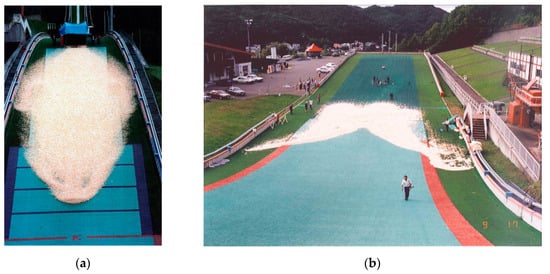
Figure 1.
Ping-pong ball granular flow experiments undertaken at the Miyanomori ski jump hill in Hokkaido, Japan [6,7,8]. (a) A ping-pong ball flow shortly after release. (b) The final deposit shape of the ping-pong ball flow, which looks like a crescent bending downslope.
To simulate the characteristics of snow avalanches, such as the flow thickness, flow speed, and run-out distance, models have an ingenious friction law. RAMMS [10] is probably the best-known model among many numerical models for snow avalanches. This model is based on the Voellmy friction law [11]. Some other models based on the work by [12,13] use a Mohr–Coulomb-type failure criterion, characterized by a single bed friction angle for the bed friction law. The Savage–Hutter model is also incorporated into a numerical model called Titan2D [14]. In Titan2D, the Savage–Hutter model was extended to be used with an arbitrary 3D-terrain model. Titan2D is widely used for simulating debris flows, volcanic pyroclastic flows, and snow avalanches [15,16,17,18].
Although constructing a numerical model to capture major characteristics of granular flows is a challenge, some studies have successfully reproduced key morphological features such as levees or channel structures as observed in nature and the laboratory, using a depth-averaged model with a velocity-dependent friction law (e.g., [19,20]). Maeno et al. [21] applied an inertia-dependent flow friction model (I-dependent model) to study the slumping of a granular mass on a slope in the laboratory, and showed that the model can work well to reproduce these phenomena. The characteristic of the I-dependent model is that the friction is controlled by the inertia number I, and I itself varies with shear rate, particle diameter, and pressure, as explained in the next section. This type of friction model incorporates the parameters related to the particles and may be useful to simulate granular flows in various situations. Intriguingly, the simulation results of the I-dependent model reproduce the crescent shape, while Titan2D does not (Figure 2). This suggests that the I-dependent model could be useful to reproduce the ping-pong ball experiments as well. Originally, the model implements inertia-dependent flow friction laws derived from experimental works such as [19,22,23]. With this background, we have started to think about using the I-dependent model for simulating snow avalanches. Some encouraging examples were presented by [24] and a Swiss group [25,26]. They modeled the relation between shear and normal stresses. Nishimura and Maeno [24] measured cohesion based on their chute flow experiments using real snow particles. They proposed using the Bingham relation for shear and normal stresses among other shear–normal stress relations. Being inspired by their study, the Swiss group repeated experiments with their larger slope using both wet and dry snow particles. They also measured cohesion and suggested a new relation for the shear and normal stresses similar to the I-dependent model. Counting the Swiss shear–normal stress relation in the numerical simulation, they successfully reproduced the crescent shape feature of real snow avalanches [26]. Their outcomes encouraged us to work with the I-dependent model by applying it to real snow avalanches. Recently, Issler et al. [27] pointed out that I-dependent rheology has many features that are observed in the dense part of snow avalanches. With these encouraging examples, we conducted a comparison between our model results and the ping-pong ball avalanche results.
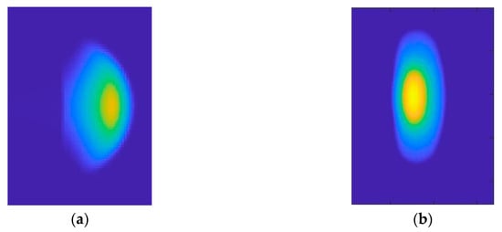
Figure 2.
Numerical simulation results of the ping-pong ball experiments. The flow direction is from left to right. Deposit shape predicted by (a) the I-dependent model with 30° and = 20°; (b) Titan2D with = 30° and = 20°.
In this paper, we discuss the effects of particle diameter in the model which was not clearly discussed in [21] and compare it with the experimental results of the ping-pong ball experiment. We explain the I-dependent friction model and its numerical model in Section 2. The method of verifying the flow model and searching for the appropriate parameter values by comparison with the ping-pong ball experiment results is also shown in Section 3. The simulation results are shown in Section 3. The effect of particle diameter and the model characteristics are discussed in Section 4. Concluding remarks are presented in Section 5.
2. Model and Method
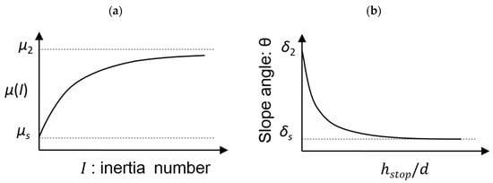
The numerical model of granular flow proposed by [21] featured a dense flow layer at the bottom of the granular flow. Their equations of mass and momentum conservation use a depth-averaged assumption with the latter conservation including a source term which contains the basal shear stress, T. The basal shear stress T includes the friction coefficient μ, which is a dimensionless parameter defined as the ratio of shear stress and normal stress (, shear stress; normal stress). μ depends on the inertia number I. Therefore, we call the numerical model of [21] the “I-dependent model”, while other researchers refer to this model as the “” model (e.g., [23]). In the I-dependent model, the relationship between the friction coefficient μ, and the inertia number I was derived by [28] as follows,
where I0 is a constant that is derived based on the experimental results. The value of I0 for glass beads is approximately 0.3 according to [22], and we use this value even though our material is different. For the constant friction model, and are defined as
where and are the upper and lower limits of slope angles in Figure 3 of [29] expressed as θ (°). In fact, the relationship of Equation (1) was derived based on the experimental results of [29] (the first researcher to conduct this experiment) and other following studies (e.g., [22,28,30]). Numerically, a granular flow can be treated as an incompressible and depth-averaged flow. Thus, the inertia I is expressed in its depth-averaged form using the depth-averaged velocity , particle diameter d, gravity acceleration , slope inclination angle θ, and flow thickness h as
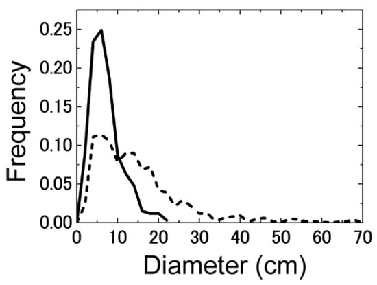
Figure 3.
The particle diameter of snow avalanche deposit. The solid line shows the graph of a dry snow avalanche and the dotted line shows a wet avalanche. Both graphs show a peak in the 0–10 cm range [33].
The derivation of Equation (3) was explained in detail in [21,22]. The governing equations such as mass conservation and momentum conservation are based on the shallow water theory. We explain the governing equations by referencing Titan2D, which is also a shallow water model. The global equations are
where vectors , , and are as follows:
where Vx and Vy are the flow velocities in the x and y directions, respectively. The first equation is a mass conservation equation, and the second and the third equations are momentum conservation equations in the x and y directions. The x-axis represents a downslope direction on a plane parallel to the slope in our simple terrain similar to a ski jump hill (Figure 1). The y-axis represents the width of the slope. C0 is a constant showing a clear difference between the I-dependent model and Titan2D, being defined as in the I-dependent model, and as in Titan2D, where denotes an earth pressure coefficient. Moreover, the source term of Equation (4) “” shows the features of each numerical model because this term includes friction effects. The source term of the I-dependent model is
with and , where denotes the bulk density and and denote the basal shear stress components defined as T = (). The source term of Titan2D is provided here as a reference.
where and are gravity accelerations in the x and y directions, and ϕint and ϕbed are the internal and bed frictions. As seen in these equations, the source term of Titan2D clearly consists of the gravity term, internal friction term, and basal friction term, while the source term of the I-dependent model consists of the gravity term and shear stress terms of Tx and Ty, neglecting the internal friction term (see [31] for another I-dependent model that retains internal friction). This includes of Equation (1). According to these equations, and of the I-dependent model are physically different from ϕint and ϕbed of Titan2D. We need to be careful of this difference when we discuss these two models. The stopping criterion is applied using the threshold value of the shear stress defined as
If the norm of the basal shear stress is smaller than , the velocity becomes 0.
Numerical simulations are implemented using the finite volume method developed by [21]. They were based on the code of [32], but with the source term calculation from the Runge–Kutta method.
The parameters for simulating snow avalanches were considered based on the experimental and observational results. Firstly, particles in real snow avalanche flows were measured by [33]. They measured the particle diameter of snow avalanche debris in snow deposits. Graphs of the particle diameter are shown in Figure 3. These histograms of wet and dry snow particles have a peak between 0 and 10 cm. The graph of the wet avalanche particles shows a wider variation and many particles are 10–20 cm in diameter. Snow avalanche particles increase in size [33] or are fractured by collision [34] during the flow. The observed snow in Figure 3 was both wet and dry, and the peaks of both particles are within the range of 0–10 cm. Moreover, the median of the grain size distributions, which are also taken from the field observation of the Swiss avalanche sites, was within 5–16 cm [35], and the order was similar to that measured by [33]. Therefore, we used a particle diameter from 0.1 mm to 10 cm as an input parameter value.
According to [21], their simulation results with δs = 22–26° and δ2 = 28–32° were in agreement with the experimental results carried out using glass beads. Even though our experiments involved ping-pong balls or snow, and not glass beads, we used their values to define the input values of the friction angles δs = 20–26° and δ2 = 28–34°, because the best estimates of the ping-pong balls or snow material are not known.
3. Results
Here, the numerical simulation results are shown: one investigating the particle diameter effect of the I-dependent model and the other a comparison with the ping-pong ball experiment [8], where the effects of friction angles were also considered.
3.1. Particle Diameter and Flow Characteristics
The diameter of snow avalanche particles is variable as shown in Figure 3. Therefore, we investigated the dependency of flow characteristics on the particle diameter.
Firstly, we have conducted numerical experiments using various size particles and slopes to examine how particle diameter d affects the flow shape. In these numerical experiments, we used slopes which have steep angles (47°, 37°, 26°, and 15°) at the releasing position, and thus, the release heights (corresponding to the “total vertical drop” in [9]) vary as 2190, 1640, 1090, and 550 m respectively. The steepness gradually decreases with distance from the releasing position, and finally, the slopes become flat (Figure 4). A cylindrical pile, which has a 50 m radius and a 10 m height, is set at the release position and the granular flow starts from rest. The model parameters are chosen as and .
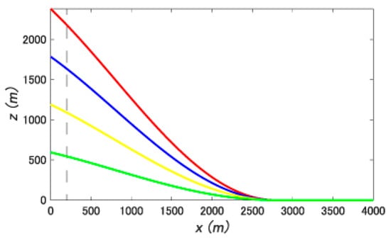
Figure 4.
Slopes used in the simulation for revealing the effect of particle diameter d. The broken line shows the particle release position. The steepness of the slope at the release position was 47° (red), 37° (blue), 26° (yellow), and 15° (green) and the release heights were 2190, 1640, 1090, and 550 m, respectively.
The final resting shape becomes elongated in the direction perpendicular to the flow direction and tapers downstream as the particle diameter becomes smaller (Figure 5). In other words, the smaller the particle diameter is, the clearer the crescent shape becomes visually. Our analysis of the width (elongation perpendicular to the flow direction) and tail length (stretch length in the flow direction) is shown in Table 1. As shown in Table 1, both the width and tail length become larger as the particle diameter decreases.
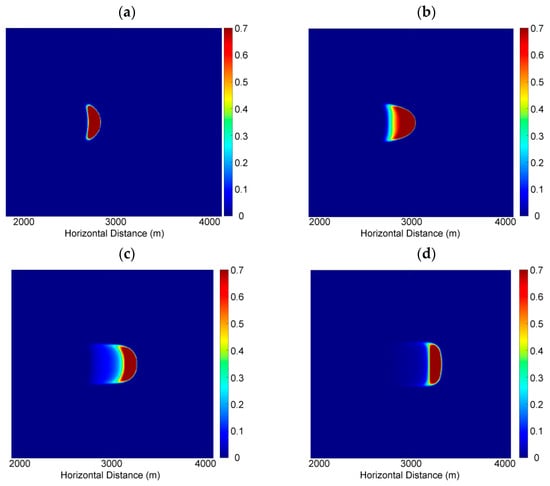
Figure 5.
The final resting shape of the flows. Colored bars show the flow thickness in meters. The shape variation depending on the particle diameter was simulated with the I-dependent model on the 47° slope (at the release position). Cylindrical granular piles were set at the release positions initially and the flow started automatically. The particle diameters are (a) 10 cm, (b) 1 cm, (c) 1 mm, and (d) 0.1 mm.

Table 1.
Width and tail length of the final resting shape of simulated granular flows. The width and tail length are measured using the simulation results shown in Figure 5.
The flow front positions are plotted against time for the two slopes, which have slope angles of 47° and 26° at the release position (Figure 6). The flow front velocity is faster when the particles are smaller. The comparison of flow front positions shows that the relationship between the velocity and particle diameter is maintained even when the slope inclinations and release heights change (Figure 6a,b).
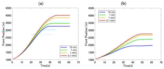
Figure 6.
A numerically simulated variation of the flow front positions over time. Simulations were implemented for a flow on the (a) 47° slope (at the release position) and (b) 26° slope (at the release position).
3.2. Comparison with the Ping-Pong Ball Experiment
Secondly, numerical simulations were implemented in order to verify whether this model can reproduce results from ping-pong ball experiments. To simulate ping-pong ball flows on the ski jump slope, we used the slope data of [7] (Figure 7).
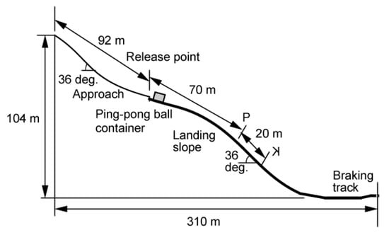
Figure 7.
Schematic diagram of the Miyanomori ski jump hill modified from [7]. At the release position, ping-pong balls were released from a container.
The height difference between the release position and the flat plane at the bottom of the slope was approximately 70 m. The slope inclination was 18° at the release position and 36° at the steepest part. In total, 28 simulations were run (four δs cases and seven δ2 cases) as shown in Table 2. In our simulation, a cylindrical pile, which has a 5 m radius and a 5 m height, was released. In order to study the effect of particle diameter on our numerical model, we used five different sizes of particles—10 cm, 3.8 cm, 1 cm, 1 mm, and 0.1 mm—though the diameter of the real ping-pong ball used in the experiment was 3.8 cm. Therefore, we have carried out 140 calculations for simulating the ping-pong ball experiment.
Table 2.
Conditions of simulations for ping-pong ball flows.
The final shapes of the ping-pong ball deposits for = 20° and = 29° (case 05) are shown in Figure 8 as an example. This variation of the flow shape for different particle sizes is common for all other cases; a crescent shape is clearer for smaller particle sizes. In order to compare the simulated results and experimental results, we calculated the flow front velocity from the simulation as it was the only parameter that could be obtained from both ping-pong ball flows and simulated flows. To have an intuitive image of the difference between experimental flows and simulated flows, we show the graphs of the flow front velocity, including experimental and simulated results for = 29° as an example (Figure 9). Our simulation results show that the flow is decelerated for the first moment and accelerated after deceleration, showing a smooth and convex parabolic curve. Plots of the raw data show a decrease in velocity around the first 10 m (Figure 9), although the smoothed curve ignores this reduction in velocity. Therefore, the qualitative feature of the velocity is the same among experimental and simulated results. These profiles also show that the velocity distributions of smaller particle flows are always larger than those of large particles, which agrees with the simulated results using the various particle diameters, as shown in Section 3.1.
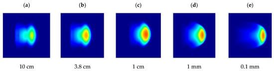
Figure 8.
The final deposit shape of simulated flows for δ2 = 29° and δs = 20° (case 05). The particle diameters are (a) d = 10 cm, (b) d = 3.8 cm, (c) d = 1 cm, (d) d = 1 mm, and (e) d = 0.1 mm.
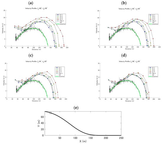
Figure 9.
Comparison of the flow front velocity in the case of δ2 = 29°. (a) δs = 20°, (b) δs = 22°, (c) δs = 24°, and (d) δs = 26°. In each graph, the simulation results of d = 10 cm (blue circle), d = 3.8 cm (sky blue star), d = 1 cm (green square), d = 1 mm (yellow triangle), and d = 0.1 mm (red diamond). Raw (black dots) and smoothed (green line) experimental results are included. (e) The slope profile used to simulate the ping-pong ball simulations. A square in the slope figure shows the position of the ping-pong ball container. Raw and smoothed data of front velocity are from [8].
Despite the similar qualitative features, the simulated velocities show a large difference from the experimental profiles with = 29°. This discrepancy becomes smaller when both and are increased. As the simulated flow of smaller particles is faster than that of larger particles, the larger the particles become, the better the velocity fits with the experimental results.
When we focus on the real ping-pong ball size (3.8 cm), the velocity distributions closely resemble the experimental results in the case of δ2 = 32° and δ2 = 33° (Figure 10). The maximum velocity of the experimental results is especially similar to that in the simulated cases of {δs = 26°, δ2 = 32°} and {δs = 20°, δ2 = 33°}.
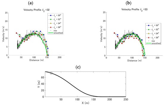
Figure 10.
Comparison of the flow front velocity in the case of a particle diameter d = 3.8 cm. (a) Simulations with δ2 = 32°. (b) Simulations with δ2 = 33°. In each graph, the simulation results of δs = 20° (blue circle), δs = 22° (green square), δs = 24° (yellow triangle), and δs = 26° (red diamond). Ping-pong ball experimental results of raw (black dots) and smoothed data (green line) are included. (c) The slope profile used to simulate the ping-pong ball simulations. A square in the slope figure shows the position of the ping-pong ball container. Raw and smoothed data of front velocity are from [8].
3.3. Error Analysis
To investigate the best fit and convergence conditions of the experimental and simulated velocity distributions, we carried out an error analysis using these velocity data. The error was calculated by interpolating the velocities with a distance resolution = 1 m as a standard across all simulations. We applied spline interpolation to the simulated velocity. The relative error is calculated as
where is the velocity of the experimental result and is the velocity of the simulated results at each distance. The index denotes each position of the distance where the interpolated values were chosen with a resolution, = 1 m.
The relative error of velocity for each particle diameter (10 cm, 3.8 cm, 1cm, 1 mm, and 0.1 mm) was plotted on the given and area (Figure 11). The sets of parameters which give the best fit for each particle diameter are {d, , , Er} = {10 cm, 20°, 32°, 0.1486}, {3.8 cm, 24°, 32°, 0.1665}, {1 cm, 26°, 32°, 0.1860}, {1 mm, 26°, 34°, 0.2442}, {0.1 mm, 26°, 34°, 0.4080}. According to these numbers, we could see that the larger the particle diameter is, the better the velocity of the experimental and simulated results fit. In order to clarify how the minimum relative error of the velocity varies with the particle diameter, these minimum error values were plotted against the particle diameter (Figure 12).
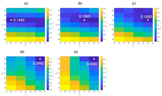
Figure 11.
The relative error of velocity on the δs and δ2 plane for particle diameters (a) d = 10 cm, (b) d = 3.8 cm, (c) d = 1 cm, (d) d = 1 mm, and (e) d = 0.1 mm. The white circles show the minimum error position in each plane. The number in each plane is the minimum relative error value.
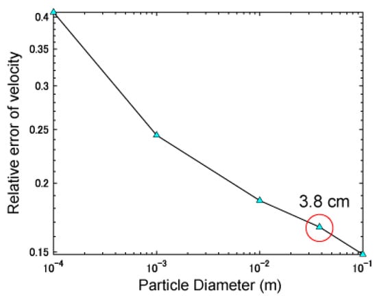
Figure 12.
Minimum relative errors of velocity between the simulated and experimental velocities against the particle diameter d. The simulations are implemented with ° and .
The graph in Figure 12 is a log–log plot of the relative error against the particle diameter. We expected to have a convergence of the relative error of velocity, although it does not show a flattening of the curve at the bottom. This means that the error can be smaller if the particle diameter is larger and the convergence of the relative error does not appear within the calculated range.
4. Discussion
In the proceeding section, we have shown the results of the numerical simulations with the I-dependent friction model. Furthermore, we have compared the simulation results with the experimental result of a ping-pong ball avalanche experiment on a ski jump hill. Based on these results, we discuss the reproducibility of the shape and flow front velocity in terms of the effect of particle diameter d and two model parameters, the upper and lower limits of slope angles allowing steady flows, and .
4.1. Shape Reproducibility
The flow shape obtained in the numerical experiments has the following tendency—the more elongated and trailed off the flow deposit shape becomes, the more clearly the crescent shape emerges (Figure 5). This is probably due to the inertia number definition , which is originally a ratio of the timescale and , where is the confinement timescale and is the typical time of deformation [22]. Let us assume that there are two particle layers, one above the other. is the travel time of distance d laterally within a moving flow, and the is the time for a particle to drop into the hole below. This is to say that all particles, whether piling up, resting, or proceeding, are controlled by the inertia number I. Then, whether or not this particle behavior produces a crescent shape depends on the particle diameter d. Based on the equations, the friction coefficient μ increases with the inertia number I (Equation (1)), and it increases with the particle size d as well (Equation (3)). The flow becomes more mobile as the particle size d decreases. The final resting shape width becomes larger and the tail becomes longer as the flow spreads.
The comparison of the flow deposit shape between the ping-pong ball experiment result and the simulation results showed that the flow deposit shape is clearly a crescent shape with the particle size d = 1 and 0.1 mm. However, when we used the true particle size of the ping-pong ball (d = 3.8 cm), the simulated results did not show the clear bending shape as observed in the experiment (Figure 1b). There might be a significant discrepancy between the numerical model and the ping-pong ball flow. We will discuss this point in more detail later (Section 4.2).
4.2. Velocity Reproducibility
The velocity of the simulation is also dependent on the particle size d. The smaller the particle size is, the faster the flow becomes (Figure 6) for fixed values of and . Based on the simulations with various slope angles, this tendency is qualitatively the same even if the slope angle and the release height change (Figure 6a,b). The inertia number effect also appears in the relationship between the flow velocity and the particle diameter. Mobility or deformability is explained as the competition of particle movement going forward and dropping in the gap between granular flow, and thus, the flow becomes more mobile and faster when the particle size d decreases. Ultimately, the simulated flow velocity is higher than the ping-pong ball velocity when the particle size d is small. In order to find the best fit condition, we had to compensate for the reduced friction from smaller particles (due to the lower value of at a given velocity and flow depth) by increasing both and . Therefore, in the cases where the particle size is d = 1 and 0.1 mm, the minimum relative error emerges at the largest value and , which is shown at the top right cell in Figure 11d,e.
Drawing a graph of the relative error against the particle diameter (Figure 12), the best fit particle size (10 cm) is found to be larger than the real particle size of a ping-pong ball. There are several possible reasons for this discrepancy: (1) the ping-pong ball flow is not suitable for verifying dense granular flow behavior, (2) the rheology is ill-posed mathematically as [36] suggested, and (3) the value of the parameter I0 for ping-pong ball flows differs substantially from 0.3 and needs to be calibrated or extracted from laboratory experiments with ping-pong balls.
An issue pointing towards possibility (1) as an explanation is the transition of the front of the ping-pong ball flow to a semi-dilute state, as ping-pong balls were jumping and colliding with each other during the descent. A picture of the ping-pong ball experiment (Figure 1a) shows that the flow front became semi-dilute and two “eyes-like” features appeared at the flow front. Aerodynamic drag on the light ping-pong balls becomes non-negligible at moderate velocities; consequently, the ping-pong ball flow is slower than the simulated dense flow with the same particle diameter.
The second possibility, that the rheology is ill-posed in a certain condition, was recently studied by [36]. They showed that the I-dependent friction model is mathematically ill-posed for sufficiently large or sufficiently small values of I/I0. Some of our simulations are in the unstable region, but no signs of numerical instability have been observed (perhaps due to a sufficient degree of code-inherent numerical viscosity). Therefore, it appears unlikely that ill-posedness of the model equations can explain the mismatch between the best-fit particle diameter and the real particle diameter.
The third possibility, that the material difference needs new experiments to calibrate the model, should always be checked when we have new material. Values used in our simulations were based on the experimental result with glass beads. It would be most valuable to have directly determined values of the friction parameters and or the corresponding angles and (Figure 13) and the shearing scale I0. Unfortunately, our attempts at measuring the angle , which can be viewed as a repose angle, for ping-pong balls, have failed so far.
Obtaining values of these parameters for snow avalanches presents even larger challenges: snow deforms, melts, sticks, and makes larger grains [38]. It remains to be seen whether experiments similar to those of Pouliquen and Forterre [19] can be carried out with real snow. The chute experiments reported in [39] represent a first step in this direction.
Moreover, it will be important to understand the dynamics of granulation because the granulation changes the effective particle size of the flow. Further experimentation along the lines suggested by [34] should be most valuable in this respect.
We conclude from this discussion that the discrepancy between the real and best-fit particle sizes is most likely due to the transition of the flow front to a semi-dilute regime and the non-negligible effect of aerodynamic drag on the ping-pong balls. Further work is needed to estimate the extra retarding force of aerodynamic drag and to include it in the model as an extra source term.
Furthermore, it is essential to validate this model with observed data in order to apply this model to the realistic snow avalanches. Avalanche velocity was estimated based on the seismic signals (e.g., [18,40,41]), and the Doppler radar measurements [42,43,44]. We can use these observational results for the validation of the model. Gauer [45] revealed the scaling behavior of the front velocity, which is proportional to the square root of the fall height. It might be interesting to see if the I-dependent rheology can reproduce such velocity features of snow avalanches.
5. Conclusions
We have presented a numerical model using an I-dependent friction model [21], which was developed based on the experimental approaches of granular flows done by Pouliquen and collaborators (e.g., [19,29,37]). After conducting a parameter study with a variable particle diameter d, we clarified that the smaller the particle is, the more the granular flow becomes mobile, resulting in a more widely spreading faster flow.
The deposit shape of the flow is so dependent on the particle diameter d that the real ping-pong ball diameter could not reproduce the crescent or bending shape of the flow. Unexpectedly, the simulated flow front velocity with smaller particles does not agree with the experimental flow front velocity even though the crescent shape reproduced well with the smaller particles. This discrepancy was mainly caused by the difference in properties of the various materials. The ping-pong balls in the flow jumped and collided with each other, since most of them were affected by aerodynamic drag. Ping-pong balls have a different property than glass beads, but might be similar to the snow avalanche property, because snow avalanches are sometimes dilute, sometimes dense, and sometimes in an intermediate regime.
Considering the application of the I-dependent model to the snow avalanches, we should study the snow avalanche property in macro and micro scales. The mean particle diameter d in a snow avalanche changes during the event. Flow experiments using real snow are expected to provide more realistic values for the two critical slope parameters and . Additionally, I0 should be chosen on the basis of experiments, rather than using the value 0.3 appropriate for glass beads.
With these experiments and improvement of the numerical code instability, it may be possible to apply this model to practical simulations in order to predict the run-out distance and affected area of snow avalanches. For the next step, it will also be necessary to improve the usability of the model.
Author Contributions
Conceptualization, K.T., F.M. and K.N.; methodology, F.M. and K.T.; software, F.M.; validation, K.T.; formal analysis, K.T.; investigation, K.T.; resources, K.N.; data curation, K.N.; writing—original draft preparation, K.T.; writing—review and editing, F.M. and K.N.; visualization, K.T.; supervision, K.N.; funding acquisition, K.N. All authors have read and agreed to the published version of the manuscript.
Funding
This work was supported by a Japan Society for the Promotion of Science (JSPS) KAKENHI Grant (15H02992).
Acknowledgments
We thank anonymous reviewers and editors for their useful comments and advice. We also appreciate Dieter Issler for his encouragement. We thank Richard W. Jordan for checking our English.
Conflicts of Interest
The authors declare that they have no conflict of interest.
References
- Lied, K.; Bakkehøi, S. Empirical calculations of snow-avalanche run-out distance based on topographic parameters. J. Glaciol. 1980, 26, 165–177. [Google Scholar] [CrossRef]
- Sovilla, B.; Margreth, S.; Bartelt, P. On snow entrainment in avalanche dynamics calculations. Cold Reg. Sci. Technol. 2007, 47, 69–79. [Google Scholar] [CrossRef]
- Gauer, P.; Issler, D. Possible erosion mechanisms in snow avalanches. Ann. Glaciol. 2004, 38, 384–392. [Google Scholar] [CrossRef]
- Keller, S. Measurements of powder snow avalanches laboratory. Surv. Geophys. 1995, 16, 661–670. [Google Scholar] [CrossRef]
- Greve, R.; Hutter, K. Motion of a granular avalanche in a convex and concave curved chute: Experiments and theoretical predictions. Philos. Trans. R. Soc. Lond. Ser. A Phys. Eng. Sci. 1993, 342, 573–600. [Google Scholar]
- McElwaine, J.; Nishimura, K. Ping-pong ball avalanche experiments. Ann. Glaciol. 2001, 32, 241–250. [Google Scholar] [CrossRef]
- Nishimura, K.; Keller, S.; McElwaine, J.; Nohguchi, Y. Ping-pong ball avalanche at a ski jump. Granul. Matter 1998, 1, 51–56. [Google Scholar] [CrossRef]
- Ogura, T.; McElwaine, J.; Nishimura, K. Drag Forces and Ping-Pong Ball Avalanches. J. Jpn. Soc. Snow Ice 2003, 65, 117–125. [Google Scholar] [CrossRef]
- McClung, D.; Schaerer, P.A. The Avalanche Handbook; Mountaineers Books: Seattle, WA, USA, 2006; pp. 36, 88, 128. [Google Scholar]
- Christen, M.; Kowalski, J.; Bartelt, P. RAMMS: Numerical simulation of dense snow avalanches in three-dimensional terrain. Cold Reg. Sci. Technol. 2010, 63, 1–14. [Google Scholar] [CrossRef]
- Voellmy, A. Über die Zerstörungskraft von Lawinen. Schweiz. Bauztg. 1955, 73, 15. [Google Scholar]
- Savage, S.; Hutter, K. The motion of a finite mass of granular material down a rough incline. J. Fluid Mech. 1989, 199, 177–215. [Google Scholar] [CrossRef]
- Savage, S.B.; Hutter, K. The dynamics of avalanches of granular materials from initiation to runout. Part I: Analysis. Acta Mech. 1991, 86, 201–223. [Google Scholar] [CrossRef]
- Patra, A.K.; Bauer, A.C.; Nichita, C.C.; Pitman, E.B.; Sheridan, M.F.; Bursik, M.; Rupp, B.; Webber, A.; Stinton, A.J.; Namikawa, L.M.; et al. Parallel adaptive numerical simulation of dry avalanches over natural terrain. J. Volcanol. Geoth. Res. 2005, 139, 1–21. [Google Scholar] [CrossRef]
- Sheridan, M.F.; Stinton, A.J.; Patra, A.; Pitman, E.B.; Bauer, A.; Nichita, C.C. Evaluating Titan2D mass-flow model using the 1963 Little Tahoma Peak avalanches, Mount Rainier, Washington. J. Volcanol. Geoth. Res. 2005, 139, 89–102. [Google Scholar] [CrossRef]
- Charbonnier, S.J.; Gertisser, R. Numerical simulations of block-and-ash flows using the Titan2D flow model: Examples from the 2006 eruption of Merapi Volcano, Java, Indonesia. Bull. Volcanol. 2009, 71, 953–959. [Google Scholar] [CrossRef]
- Takeuchi, Y.; Nishimura, K.; Patra, A. Observations and numerical simulations of the braking effect of forests on large-scale avalanches. Ann. Glaciol. 2008, 59, 50–58. [Google Scholar] [CrossRef]
- Pérez-Guillén, C.; Tsunematsu, K.; Nishimura, K.; Issler, D. Seismic location and tracking of snow avalanches and slush flows on Mt. Fuji, Japan. Earth Surf. Dyn. 2019, 7, 989–1007. [Google Scholar] [CrossRef]
- Pouliquen, O.; Forterre, Y. Friction law for dense granular flows: Application to the motion of a mass down a rough inclined plane. J. Fluid Mech. 2002, 453, 133–151. [Google Scholar] [CrossRef]
- Mangeney, A.; Bouchut, F.; Thomas, N.; Vilotte, J.P.; Bristeau, M.O. Numerical modeling of self-channeling granular flows and of their levee-channel deposits. J. Geophys. Res. 2007, 112, F02017. [Google Scholar] [CrossRef]
- Maeno, F.; Hogg, A.J.; Sparks, R.S.J.; Matson, G.P. Unconfined slumping of a granular mass on a slope. Phys. Fluids 2013, 25, 023302. [Google Scholar] [CrossRef]
- Groupement De Recherche Milieux Divisé. On dense granular flows. Eur. Phys. J. E 2004, 14, 341–365. [Google Scholar] [CrossRef]
- Edwards, A.; Viroulet, S.; Kokelaar, B.; Gray, J. Formation of levees, troughs and elevated channels by avalanches on erodible slopes. J. Fluid Mech. 2017, 823, 278–315. [Google Scholar] [CrossRef]
- Nishimura, K.; Maeno, N. Experiments on snow-avalanche dynamics. IAHS Publ. 1987, 162, 395–404. [Google Scholar]
- Platzer, K.; Bartelt, P.; Jaedicke, C. Basal shear and normal stresses of dry and wet snow avalanches after a slope deviation. Cold Reg. Sci. Technol. 2007, 49, 11–25. [Google Scholar] [CrossRef]
- Bartelt, P.; Valero, C.V.; Feistl, T.; Christen, M.; Bühler, Y.; Buser, O. Modelling cohesion in snow avalanche flow. J. Glaciol. 2015, 61, 837–850. [Google Scholar] [CrossRef]
- Issler, D.; Gauer, P.; Schaer, M.; Keller, S. Inferences on Mixed Snow Avalanches from Field Observations. Geosciences 2020, 10, 2. [Google Scholar] [CrossRef]
- Jop, P.; Forterre, Y.; Pouliquen, O. A constitutive law for dense granular flows. Nature 2006, 441, 727–730. [Google Scholar] [CrossRef]
- Pouliquen, O. Scaling laws in granular flows down rough inclined planes. Phys. Fluids 1999, 11, 542. [Google Scholar] [CrossRef]
- Pouliquen, O.; Cassar, C.; Jop, P.; Forterre, Y.; Nicolas, M. Flow of dense granular material: Towards simple constitutive laws. J. Stat. Mech. 2006, 2006, P07020. [Google Scholar] [CrossRef]
- Baker, J.L.; Barker, T.; Gray, J.M.N.T. A two-dimensional depth-averaged μ(I)-rheology for dense granular avalanches. J. Fluid Mech. 2016, 787, 367–395. [Google Scholar] [CrossRef]
- Leveque, R.J. Finite Volume Methods for Hyperbolic Problems, 1st ed.; Cambridge Texts in Applied Mathematics; Cambridge University Press: Cambridge, UK, 2002; pp. 15–420. [Google Scholar]
- Nishimura, K. Internal structure of snow avalanches. Meteorol. Res. Note 1998, 190, 21–36. (In Japanese) [Google Scholar]
- Steinkogler, W.; Gaume, J.; Löwe, H.; Sovilla, B.; Lehning, M. Granulation of snow: From tumbler experiments to discrete element simulations. J. Geophys. Res. Earth Surf. 2015, 120, 1107–1126. [Google Scholar] [CrossRef]
- Bartelt, P.; McArdell, W. Instruments and Methods Granulometric investigations of snow avalanches. J. Glaciol. 2009, 55, 829–833. [Google Scholar] [CrossRef]
- Barker, T.; Schaeffer, D.; Bohorquez, P.; Gray, J. Well-posed and ill-posed behaviour of the μ(I)-rheology for granular flow. J. Fluid Mech. 2015, 779, 794–818. [Google Scholar] [CrossRef]
- Forterre, Y.; Pouliquen, O. Flows of Dense Granular Media. Annu. Rev. Fluid Mech. 2008, 40, 1–24. [Google Scholar] [CrossRef]
- De Biagi, V.; Chiaia, B.; Frigo, B. Fractal grain distribution in snow avalanche deposits. J. Glaciol. 2012, 58, 340–346. [Google Scholar] [CrossRef]
- Bouchet, A.; Naaim, M.; Bellot, H.; Ousset, F. Experimental study of dense flow avalanches: Velocity profiles in steady and fully developed flows. Ann. Glaciol. 2004, 38, 30–34. [Google Scholar] [CrossRef][Green Version]
- Takeuchi, Y.; Yamanoi, K.; Endo, Y.; Murakami, S.; Izumi, K. Velocities for the dry and wet snow avalanches at Makunosawa valley in Myoko, Japan. Cold Reg. Sci. Technol. 2003, 37, 483–486. [Google Scholar] [CrossRef]
- Suriñach, E.; Flores-Márquez, E.L.; Roig-Lafon, P.; Furdada, G.; Tapia, M. Estimation of Avalanche Development and Frontal Velocities Based on the Spectrogram of the Seismic Signals Generated at the Vallée de la Sionne Test Site. Geosciences 2020, 10, 113. [Google Scholar] [CrossRef]
- Gauer, P.; Kern, M.; Kristensen, K.; Lied, K.; Rammer, L.; Schreiber, H. On pulsed Doppler radar measurements of avalanches and their implication to avalanche dynamics. Cold Reg. Sci. Technol. 2007, 50, 55–71. [Google Scholar] [CrossRef]
- Rammer, L.; Kern, M.; Gruber, U.; Tiefenbacher, F. Comparison of avalanche-velocity measurements by means of pulsed Doppler radar, continuous wave radar and optical methods. Cold Reg. Sci. Technol. 2007, 50, 35–54. [Google Scholar] [CrossRef]
- Köhler, A.; McElwaine, J.N.; Sovilla, B. GEODAR Data and the Flow Regimes of Snow Avalanches. J. Geophys. Res. Earth Surf. 2018, 123, 1272–1294. [Google Scholar] [CrossRef]
- Gauer, P. Considerations on scaling behavior in avalanche flow along cycloidal and parabolic tracks. Cold Reg. Sci. Technol. 2018, 151, 34–46. [Google Scholar] [CrossRef]
Publisher’s Note: MDPI stays neutral with regard to jurisdictional claims in published maps and institutional affiliations. |
© 2020 by the authors. Licensee MDPI, Basel, Switzerland. This article is an open access article distributed under the terms and conditions of the Creative Commons Attribution (CC BY) license (http://creativecommons.org/licenses/by/4.0/).