1. Introduction
The United Nations estimate that in 2050, 68% of the world’s population of approximately 10 billion people will reside in urban areas [
1]. The continuous growth of cities in combination with future climate changes present authorities with significant challenges. In Denmark, climate models estimate that future climate changes will cause an increase in the overall amount of precipitation along with a changing precipitation pattern where more frequent cloudbursts are expected to occur [
2,
3]. As traditional urban sewer systems are designed for the present climate, the new precipitation pattern will increase the frequency of flooding in urban areas, which will hamper and destroy infrastructure, buildings and the environment [
4]. According to the European Environment Agency, an economic loss of approximately 453 billion euro can be assigned to weather and climate-related extremes in the period from 1980 to 2017 [
5]. Therefore, one of the most significant challenges for urban planners is to ensure stable disposal of waste and surface water. Consequently, over the last 20 years, there has been an increasing focus on using SUDS in cities. Implementing SUDS in surface water management plans has many benefits. Studies show that the handling of surface water using SUDS is less expensive than traditional handling using sewers [
6,
7,
8,
9,
10]. In addition, the SUDS enable urban planners to use surface water as a resource instead of a problem, e.g., surface water can be used to make cities green, counteract urban heat effect as well as restore the hydraulic water cycle in urban areas [
11,
12,
13].
One of the approaches used in Denmark is infiltration-based SUDS, such as ponds, swales, rain gardens, soakaways and infiltration trenches. The primary reason for this is that infiltration-based SUDSs are cost-effective and easy to construct, compared to many other SUDS solutions. In order to find the most suitable SUDS solution for a specific area, the ground conditions, such as infiltration capacity and groundwater conditions must be known in detail, as a site may restrict or preclude a particular SUDS solution. This is especially the case in former glaciated areas, as many glacial deposits often are highly heterogeneous, and thus, their hydrological conditions can likewise be highly variable [
14,
15]. The heterogeneity is both present within the individual units, e.g., sand lenses embodied in clay till, the presence of fractures, root holes and earthworm burrows [
15] as well as between the units. To map both the internal heterogeneity as well as the overall heterogeneity of the subsurface, very detailed studies are required, which are typically time consuming and therefore also very expensive.
Typically, the data available for urban planners when designing new urban developments is point information, such as drilling in combination with overall 2D geological maps showing, e.g., soil type, infiltration capacity, areal extent and the thickness of the individual units. This is useful for identifying overall suitable locations for infiltration but is unsuitable for describing the geological and hydrogeological conditions in sufficient detail for urban planners to be able to select the best SUDS solution [
16]. The need for on-site data remains. Furthermore, drillings are invasive and costly, making them unsuitable to map large areas in detail. To compensate for the lack of dense data derived from boreholes, geophysical methods represent an efficient and non-invasive tool for mapping both urban and rural areas [
17,
18,
19,
20,
21,
22,
23,
24]. Multiple studies throughout the last decades have shown that an empirical correlation between resistivity and lithology exists [
25,
26,
27,
28]. This correlation depends on several factors, such as water saturation, clay content, clay type, soil compaction, pore water ion content and matrix resistivity [
29]. Therefore, the same lithological unit can have a wide resistivity range [
30,
31], and thus, large-scale investigations have been conducted in Denmark in order to estimate the overall resistivity range for various lithologies. Barfod et al., [
31] have made a national resistivity atlas of Denmark in grids spanning 10 × 10 km in which lithological information from boreholes has been integrated with resistivity from various transient electromagnetic methods, thus creating resistivity histograms for selected lithologies (clay, sand and gravel). The resistivity atlas of Denmark was created for two layers; 12.5 to 25 m and 25 to 55 m, respectively, and not for the near subsurface.
For near-surface investigations, electromagnetic induction (EMI) methods have proven to be very effective in successfully mapping the subsurface [
32,
33,
34,
35]. For instance, Frederiksen et al., [
36] made a quantitative comparison of a 1000 ha coherent EMI data set and 125 boreholes showing that the EMI instrument DUALEM-421S is able to map the geology of the upper 6 m in a complex glacial environment.
To the author’s knowledge, few Danish studies have tried to establish a quantitative and/or qualitative relationship between resistivity and infiltration capacity, lithology and geotechnical tests based on large-scale data sampling. Until now, only site-specific geophysical mapping has been used to investigate the best placement of SUDSs as well as their infiltration performance in Denmark [
37,
38]. Therefore, it would be advantageous if more generic similarities between geoelectric resistance, lithology, geotechnical in situ vane tests and infiltration capacity could be achieved covering larger areas. If such compilations can be established, it can help city planners make credible decisions based on as little data as possible and choose the right combination of data types in order to create reliable planning maps. With better knowledge, optimal SUDSs can be better chosen within each area and an over-or underestimation or at worst case—the completely wrong solution can be avoided.
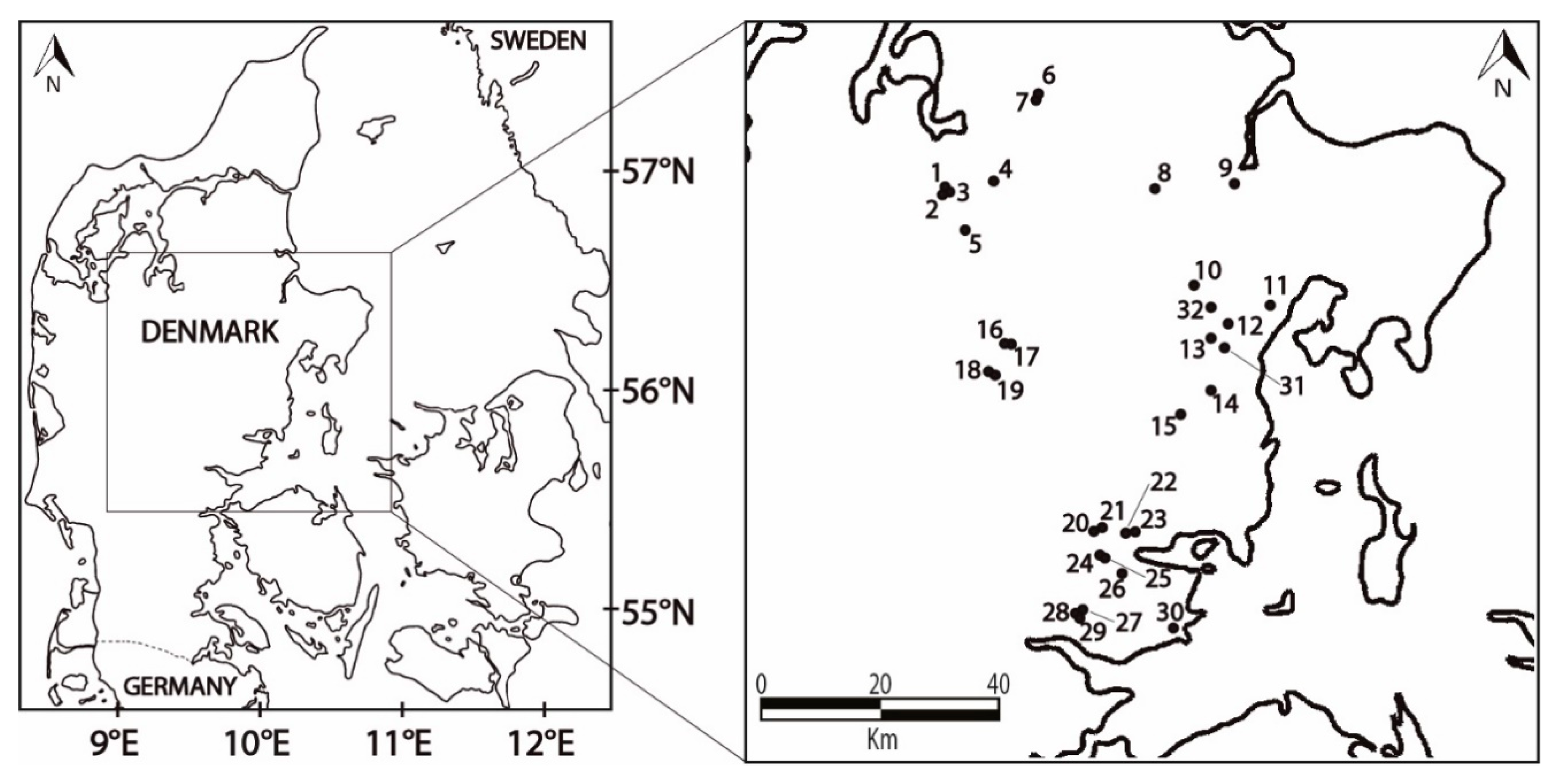
The objective of this paper is to use high-density geophysical mapping in combination with borehole data, infiltration tests and geotechnical data to outline the benefits of geophysical mapping for improved fidelity of the geological and hydrogeological characterisation at 1 m below ground surface (bgs) which is typically the construction depth of vast infiltration-based SUDS solutions in Denmark, e.g., soakaways. Data from the Central Denmark Region has been collected from 2015 and onwards from 32 different locations, and it comprises 1315 ha of high-density electromagnetic (DUALEM-421S) data, detailed lithological soil descriptions of 614 boreholes, 153 infiltration tests and 250 in situ vane tests. The data will be quantitatively and qualitatively analysed, and possible relationships between resistivity and the main lithological description and infiltration capacity and geotechnical data will be evaluated. The results will be exemplified with one case study from Provstlund, Denmark, in order to demonstrate how detailed geophysical and hydrogeological information can yield maps of the infiltration potential of urban development areas.
3. Results and Discussion
In the following section, the results of this study are presented and discussed. In order to perform a quantitative evaluation of the resistivities versus the infiltration capacity and the resistivities versus the undrained shear strength of cohesive soils, simple linear regression tests were conducted on the data. From the simple linear regression tests, we assessed whether a significant linear relationship between an independent variable X and a dependent variable Y exists. In our two tests, the dependent variable Y is either the percolation rate or the undrained shear strength of cohesive soils, and the independent variable X is, in both tests, the resistivity.
Assuming a linear relationship between an independent variable X and a dependent variable Y exists, their relationship can be expressed as follows:
where α is a constant, β is the slope of the regression line, X
i is the independent variable, and Y
i is the dependent variable. In the simple linear regression test, we tested whether the slope of the regression line is significantly different from zero using the following hypothesis test:
In order to test the hypothesis, a linear regression t-test with
n – 2 degrees of freedom was conducted using a significance level of 0.05. If the calculated
p-value was less than the significance level, the null hypothesis was rejected. If the null hypothesis were rejected, we would be able to conclude that there is a significant relationship between the independent and dependent variables. Further information about the simple linear regression test is thoroughly described by, e.g., Blæsild and Granfeldt [
46].
For qualitative evaluation of the lithologies versus resistivities and percolation rates, box plots were used.
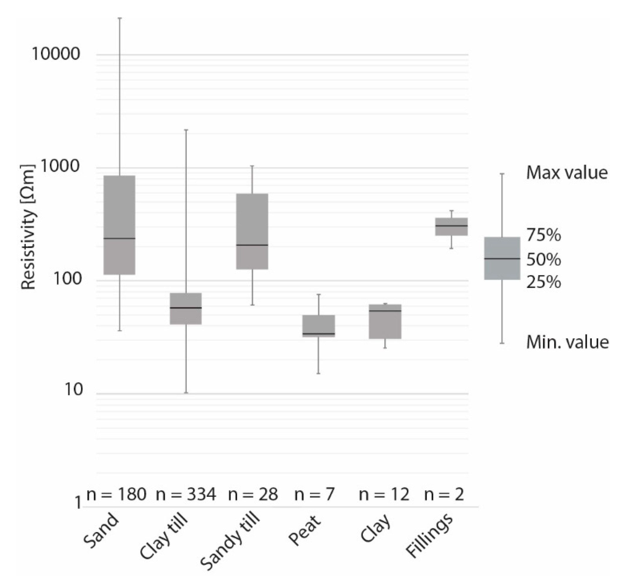
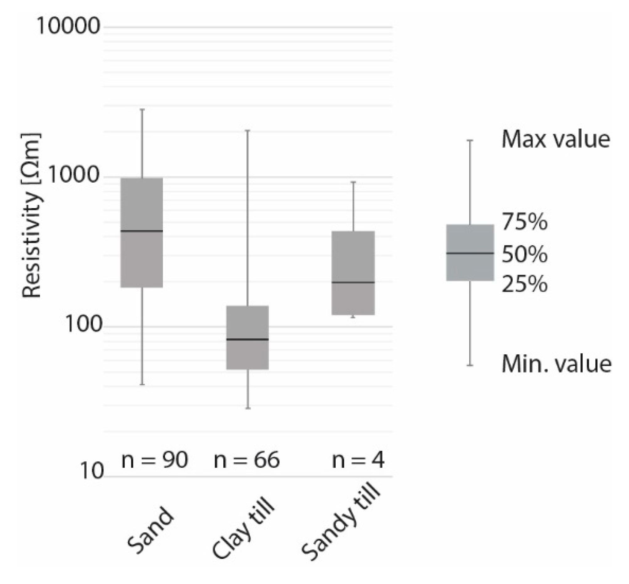
3.1. Resistivities Versus Lithology
In
Figure 2 we show the minimum, maximum and median values as well as the Q1 and Q3 quartiles for resistivities of various lithologies at 1 m bgs. for all the investigated sites. The lithologies derived from the drillings are only included if more than 75% of the soil within the depth interval, that is from 0.5 m to 1.5 m, had the same main lithology. The resistivity is obtained using the DUALEM-421S measurement nearest the drilling.
As seen from the box plot, the units cannot, with high certainty, be distinguished from each other by their resistivities alone, as the maximum and minimum resistivity range in many situations are overlapping. However, the box plot shows that sand-dominated lithologies, such as sand, sandy till and fillings have higher resistivities relative to clay and organic-dominated lithologies, such as clay, clay till and peat/organic clay. The median resistivity for sand, sandy till and fillings are 229, 201 and 296 Ωm, compared to the median resistivity for clay till, peat and clay, which are 56, 33 and 30 Ωm. For the sand-dominated deposits, the Q1 quartile for sand is the lowest with 110 Ωm, and for the clay-dominated deposits, the Q3 quartile for clay till were the highest with 76 Ωm. Hence, a cut-off value ranging from 80 to 100 Ωm can be used on a regional scale to separate the sand-dominated deposits from the clay-dominated deposits. These findings are in accordance with other Danish investigations. In Barfod et al., [
31] and in Frederiksen et al., [
36], a cut-off value of 80 Ωm was selected in order to separate the sand-dominated deposits from the clay-dominated deposits. From
Figure 2, it is also observed that it is impossible to separate sand from sandy till and fillings based on their resistivity alone, as their median resistivity values only show minor variances. Likewise, it is not possible to distinguish between clay till, peat and clay on a regional scale.
As described in the Introduction, multiple studies have described an empirical correlation between resistivity and lithology [
25,
26,
27,
28]. This correlation depends on several factors, such as water saturation, clay content, clay type, soil compaction, pore water ion content and matrix resistivity [
29]. For water-saturated clay-free porous media, such as sand, Archie’s law [
25] is valid, showing an empirical relationship of electrical conductivity to fluid (pore water ion content) and water content:
where
is the bulk conductivity of the formation,
is the fluid conductivity, and F is the formation factor. For clayey sediments, Archie’s law is not valid, as the matrix itself is electrically conductive. Multiple models have been proposed in order to account for the conductive clay minerals [
26,
47,
48]. In general, for both clay and clay-free sediments, the resistivity increases with decreasing water content [
49,
50]. As the present investigation focuses on the upper metres of the soil, the water saturation of the soil itself, as well as the groundwater level, has a strong influence on the measured resistivity. This is exemplified in the Provstlund case (described in
Section 4) where the soil samples 1 m bgs in borehole B7, B11 and B13 all were described as clay till but had measured resistivities above 500 Ωm. All the soil samples were from the unsaturated zone located on the highest elevation of the site. The very high resistivities are assumed to result from a very low water saturation of the clay till.
The local and seasonal variations of water content are assumed to be the most important obstacle in interpreting the geophysical mapping and hence hamper a regional translation from resistivity into lithology, especially when operating in the upper 1–2 m bgs, where weather conditions have a huge impact on the water saturation of the soil and the presence of groundwater. The geophysical mapping, therefore, cannot stand alone and has to be correlated with soil descriptions from boreholes and infiltration tests covering the different units identified on the site.
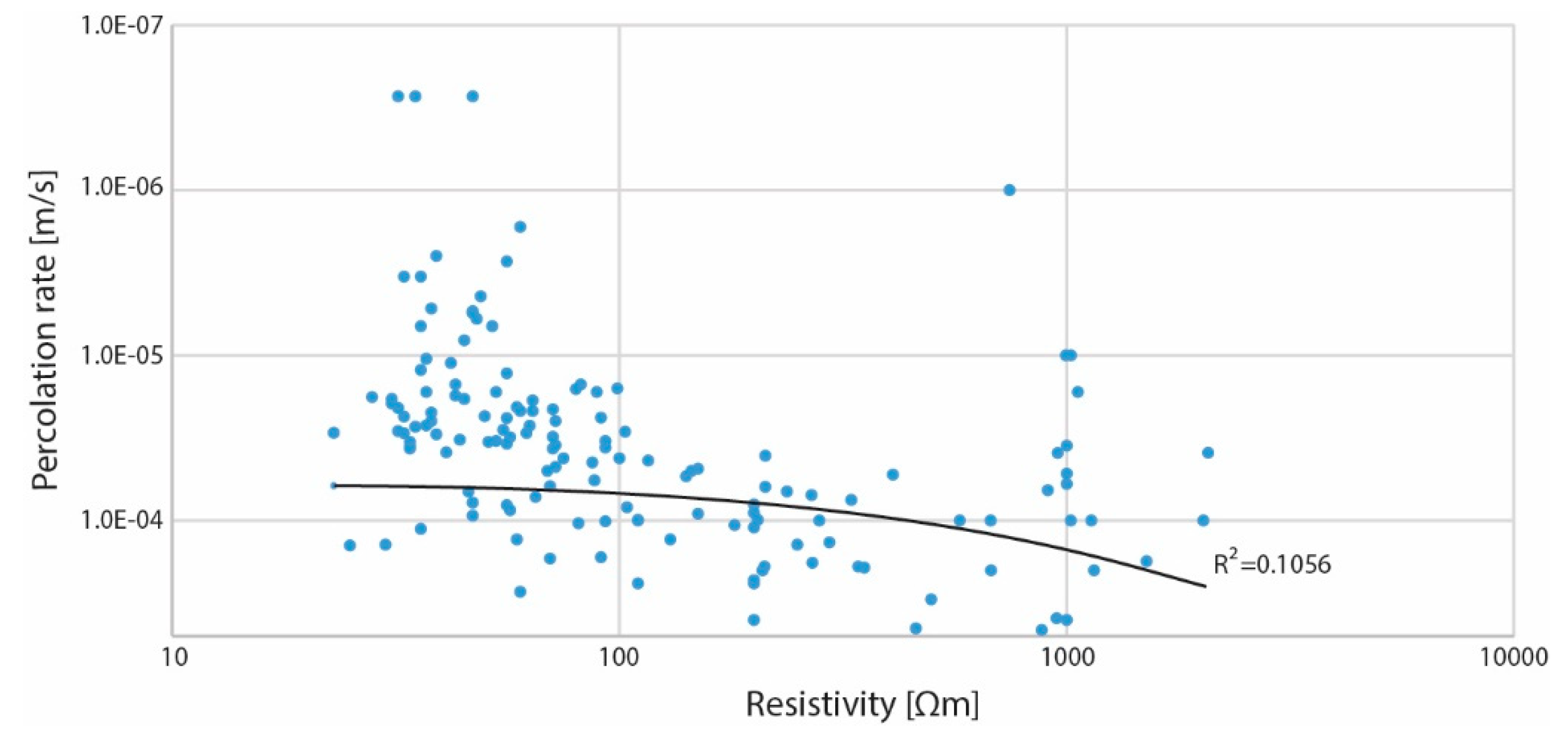
3.2. Resistivities Versus Infiltration Tests
In
Figure 3, resistivity is plotted against the percolation rates. A simple linear regression test has been conducted on the data. With a
p-value below 0.05 (5.6 × 10
−5), we reject the null hypothesis representing uncorrelated parameters. Hence, a significant relationship between resistivity and the percolation rates on a regional scale exists. The linear regression line has an R
2 value of 0.11. Thus, the measured resistivity is only able to explain 11% of the observed variations in the percolation rates. The relationship between resistivity and percolation rates is therefore considered so weak on a regional scale that in reality no meaningful relationships can be establish. Notice, as the resistivity and percolation rates are plotted as a log-linear using a logarithmic scale on the x-axis, and a linear scale on the y-axis the linear regression line is curving.
3.3. Lithologies Versus Infiltration Tests
In
Figure 3, a box plot showing the measured 147 percolation rates for various lithologies is presented. The lithologies were derived from boreholes located within 1 m from the infiltration test or from the soil sample itself. As observed from the box plot, it is possible to assign an infiltration capacity with moderate certainty based on the lithologies, as the Q1 quartiles for sand and sandy till do not overlap with the Q3 quartile for clay till. The sand-dominated units, such as sand and sandy till, have relatively higher percolation rates than the clay-dominated clay till and have median percolation rates of 9.9 × 10
−5 m/s for sand and 6.5 × 10
−5 m/s for sandy till, compared to 2.6 × 10
−5 m/s for clay till.
It is important to estimate the infiltration capacity of the different soils, as it will determine the most suitable location for the selected SUDS as well as the expected performance and size of the SUDS solution. As observed in
Figure 4, the percolation rate of both sand and clay till varies significantly. For the sand-dominated deposits, a few infiltration test outliers and the presence of fine-grained sand account for the low percolation rates of around 1 × 10
−6 m/s. The percolation rate of clay till varies from 2.7 × 10
−7 m/s to 2 × 10
−4 m/s. These results are in accordance with the results obtained by Bockhorn et al. [
38]. The variation in percolation rates for the clay till is most likely due to soil structure, the CaCO3 boundary and earthworm burrows. Bockhorn et al. [
15] investigated various factors controlling the infiltration capacity of SUDS in clay till and found that fractures, earthworm burrows and structural changes in the soil had a significant effect on the infiltration capacity.
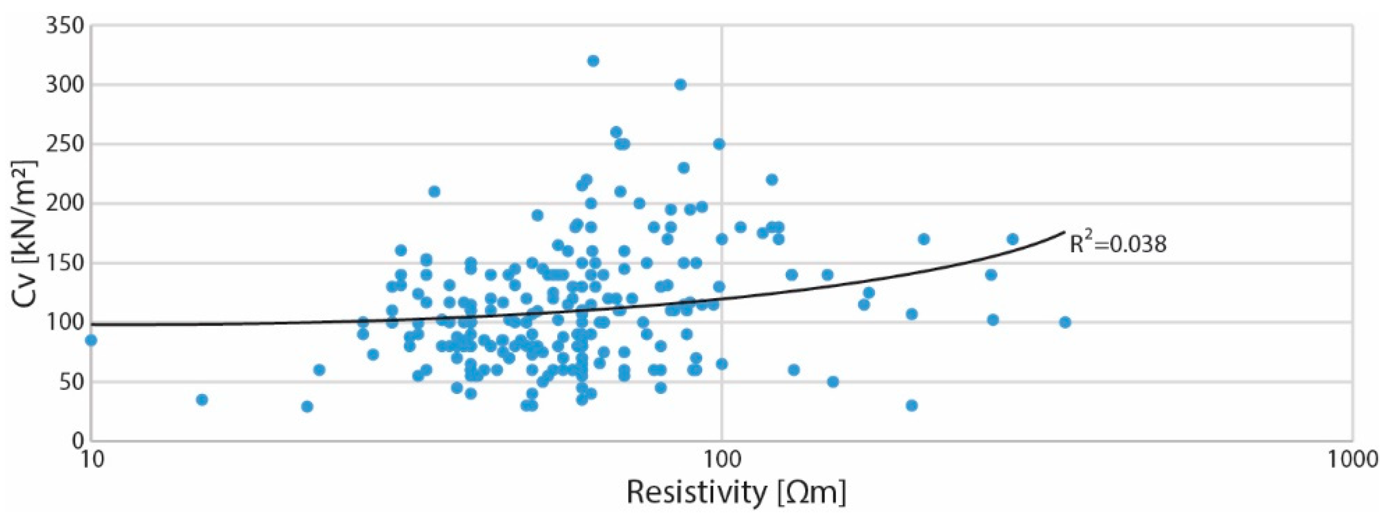
3.4. Resistivities Versus in Situ Vane Tests
In
Figure 5, resistivity is plotted against the undrained shear strength of cohesive soils obtained using the in situ vane tests. A simple linear regression test has been performed on the data. With a
p-value below 0.05 (2.3 × 10
−3), we reject the null hypothesis that there is no relationship between the two variables being studied. Hence, there exists a significant linear regression relationship between resistivity and the undrained shear strength of cohesive soils. The linear regression line has an R
2 value of only 0.038. Thus, the measured resistivity is only able to explain 4% of the observed variations in the undrained shear strength of cohesive soils, implying that the relationship between the resistivity and undrained shear strength of cohesive soils must be very weak on a regional scale, and in reality no meaningful relationships can be establish. Notice, as the resistivity and the undrained shear strength of cohesive soils is plotted as a log-linear using a logarithmic scale on the x-axis, and a linear scale on the y-axis the linear regression line is curving. In the literature, other studies have tried to establish a relationship between electrical resistivity and geotechnical data, such as standard penetration test (SPT), dynamic cone penetration test (DCPT), Atterberg limit, triaxial compression, oedometer consolidation as well as the in situ vane test [
51,
52,
53,
54,
55,
56]. As in this study, they found that the relationships are area-specific, and the results cannot be transferred from one area to another.
As seen from the quantitative analysis, no reliable relationships could be established between resistivity and the percolation rate or the undrained shear strength of cohesive soils on a regional scale. The obtained DUALEM-421S data used in the quantitative analysis has not undergone any data transformation (e.g., been sorted or binned logarithmically) before being used in the statistical analysis which most likely would have improved the R2values. However, as this study aims to investigate an immediate relationship between the measured DUALEM-421S data and the percolation rate or the undrained shear strength of cohesive soils without the use of a time-consuming and thereby more expensive data transformation process, this has not been conducted in this investigation.
Based on the qualitative analysis, the comparison of the lithologies versus resistivities and percolation rates can be estimated with moderate to high certainty on a regional scale. If used with caution, the qualitative findings can be used in the initial investigation phase in order to translate the geophysical mapping into an overall lithology and assign a percolation rate as well as an undrained shear strength of cohesive soils. If more credible relationships are necessary for the urban planners to construct, e.g., potential infiltration planning maps, then site-specific local investigations are needed. This will be exemplified with one case study from Provstlund (no. 21,
Figure 1 and
Table 1).
4. Case Study: Provstlund
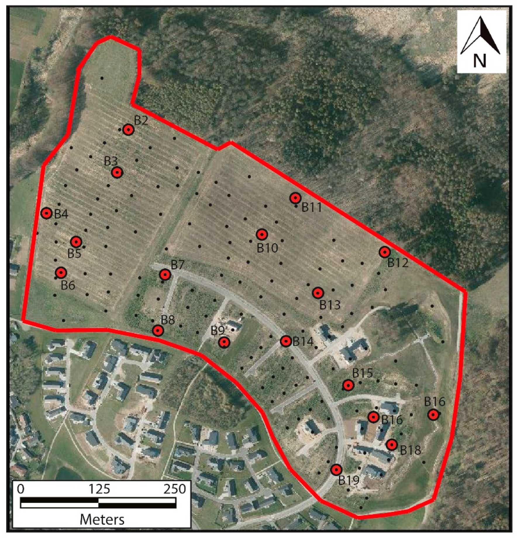
The Provstlund site is a 27 ha formerly agricultural area situated about 5 km northwest of Horsens,
Figure 6. In 2017, the site was mapped with DUALEM-421S, resulting in a total of 60,301 measurements. Of that, 4.3% of the data was removed due to noise or couplings from buried conductors, leaving a total of 57,714 measurements for the inversion. The time span of the geophysical mapping was one day.
The mean interval resistivity plots from the DUALEM-421S are plotted in
Figure 7. From 0 to 3 m bgs, the interval resistivity plots each represent the calculated mean resistivity within 50 cm of soil. From 3 to 6 m bgs, each interval resistivity plot represents 1 m. The calculated mean interval resistivity plots are blinded at the calculated penetration depth (DOI), so the number of data points decreases downwards. At the Provstlund site, the penetration depth varied from 5 to 7 m. The calculated mean resistivity is presented as points, and no kind of interpolation of the calculated values has been made. As observed in
Figure 7, high resistances (> 100 Ωm) were generally seen in the upper 1.0 m in large parts of the area. Smaller areas with medium resistances (30–60 Ωm) were seen mainly in the north-western and south-eastern parts of the area. The extent of the medium resistivity areas was typically 150 to 200 m
2. From 1 to 2 m bgs, the medium resistivity areas expanded to more continuous and larger areas. The largest areas were observed towards the southeast, central and west. From 1.5 to 2 m bgs, 1/3 of the area comprised areas with medium resistivities, and 2/3 of the area comprised areas with high resistivities. Larger contiguous high-resistivity areas were seen in the central part of the region as well as in the north-eastern corner and in the north-western and south-western parts of the area. From 2.5 m bgs to 6 m bgs, similar resistivity patterns were observed, with half the area comprising of medium resistivity and the other half of high resistivity areas. The high resistivity areas were observed in the north-western, south-western and eastern parts of the area. The north-western and south-western high resistivity areas had the same overall size and shape, whereas the eastern high resistivity area shrank in size with depth.
Within a few days of the geophysical mapping, 18 drillings, each 4 m deep, 18 infiltration tests and 19 in situ vane tests were performed. The drillings were placed in uniform resistivity zones based on the geophysical mapping results. In the additional geotechnical investigation phase, around three months after the geophysical mapping, 143 drillings ranging in depth from 4 to 6 m and 141 in situ vane tests were conducted, as shown in
Figure 6. Their placement was independent of the results from the geophysical mapping campaign.
In all the drillings, the groundwater level was observed to be situated below the terminus of the drillings, implying that it is located more than 4 m bgs. Out of the total set of drillings, 159 were described with respect to lithology and groundwater level and in 59 of the drillings the undrained shear strength was obtained. In
Figure 8, the box plot showing the minimum, maximum and median values as well as the Q1 and Q3 quartiles for resistivities of various lithologies at 1 m bgs at Provstlund is plotted. The lithologies were derived from the drillings, and the resistivity was selected from the nearest DUALEM-421S measurement.
As observed from
Figure 8, sand and clay till can be distinguished with moderate to high certainty based on their resistivities, as the upper Q3 (75%) and the lower Q1 (25%) quartiles do not overlap. On the other hand, it is not possible to clearly distinguish sandy till from either sand or clay till, as their upper Q3 (75%) and lower Q1 (25%) quartiles overlap. Thus, sandy till might be misinterpreted as sand or as clay till. The median resistivities were 445, 198 and 83 Ωm for sand, sandy till and clay till, respectively. At the Provstlund site, the differences in median resistivities for sand, sandy till and clay till were +216, -4 and +27 Ωm, respectively, compared to the regional median resistivity. The higher resistivities of sand and clay till at Provstlund were most likely due to low water saturation of the soils and low-lying groundwater level. Hence, the cut-off value between sand and clay till was set to 150 Ωm, compared to the regional scale cut-off value that is between 80 to 100 Ωm. The high difference in cut-off values between Provstlund and the regional value showed that local data sampling was necessary to create reliable translations between resistivities and lithologies.
To obtain an overview of the hydraulic capacity of the soil layers in the area, 18 infiltration tests were performed (see
Figure 6). The infiltration tests were performed next to the boreholes so that the results could be compared with the geological descriptions, as in
Table 2. To obtain a representative measurement, the topsoil layer (approx. 0.5 to 1 m) was excavated before performing the infiltration tests, so that all tests were made on undisturbed soil.
Table 2 shows the results of the infiltration tests and the geophysical mean resistivity values measured in the depth range 0.5 to 1 m, which represented the depth the infiltration tests were performed in. In general, a very good correlation was seen between areas with high resistance, a sandy lithology from the boreholes and high percolation rates spanning from 1 × 10
−4 m/s to 4 × 10
−5 m/s,
Table 2. However, boreholes 11 and 13 should be mentioned; both showed high resistances but were described as moraine clays and had percolation rates of around 4 to 5 × 10
−5 m/s, which was interpreted as dry moraine clays. The remaining boreholes were all described as having moraine clays in the upper 1 m, which correlated well with the low resistances (30–80 Ωm) and percolation rates spanning from 5 × 10
−5 m/s to 5 × 10
−6 m/s. All the percolation rates obtained at the Provstlund site are similar to the regional percolation rates (see
Figure 4).
A total of 46 in situ vane tests were conducted in Provstlund in order to achieve the undrained shear strength of cohesive soils. A simple linear regression test was conducted on the data. With a p-value above 0.05 (0.69), we cannot reject the null hypothesis that there is no relationship between the two variables being studied. Hence, at the Provstlund site, we cannot conclude whether or not there is a significant linear relationship between resistivity and the undrained shear strength of cohesive soils. Thus, in order to achieve a reliable overview of the undrained shear strength, multiple in situ vane tests need to be conducted.
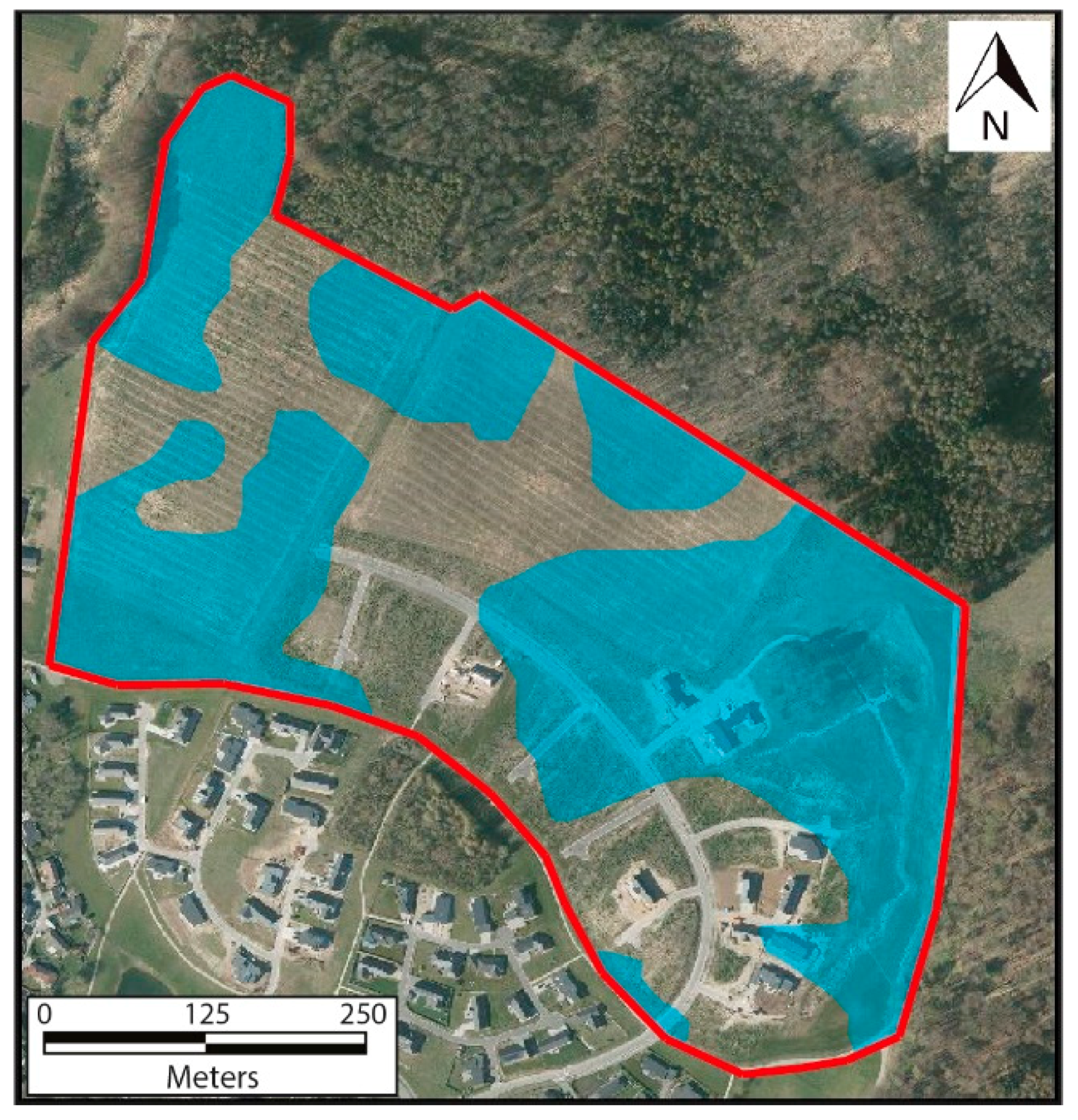
Based on the geophysical mapping, soil descriptions and infiltration tests, high-resistivity areas can be interpreted as sand-dominated areas having percolation rates spanning 2 × 10
−5 m/s to 1 × 10
−4 m/s, corresponding to medium to fine-grained sand. Similarly, low resistivity areas can be interpreted as clay-dominated areas with percolation rates between 5 × 10
−5 m/s to 5 × 10
−6 m/s, corresponding to clay tills. Based on the data, a planning map for the Provstlund site can be created showing areas suitable for the infiltration of surface water, as in
Figure 9. The geophysical mapping, soil descriptions from boreholes and infiltration tests provide information on the volume, areal extent and hydraulic properties of various soils, and the groundwater head measurements provide information about the volume of the unsaturated zone. Combining the data enables city planners to construct planning maps with precise estimates of the most suitable areas for infiltration as well as the volume of free space in unsaturated soil for infiltrated water. As observed from
Figure 9, the most suitable areas for infiltration are located throughout the Provstlund site, with the biggest continuous areas in the eastern and south-western parts of the site. Medium-sized areas are observed in the northern part of the site and the smallest area in the south. The areas are characterised as having high resistivity areas, boreholes showing sand-dominated soil descriptions, infiltration capacities of 2 × 10
−5 m/s to 1 × 10
−4 m/s and a thickness of more than 4 m in the unsaturated zone.
A planning map showing the most suitable areas for infiltration provides authorities with a powerful tool when planning the future urbanisation of the site. The map enables them to organise the areas based on holistic water cycle management, focusing on the best SUDS solution for the area, instead of having the individual citizens handling their own rainwater, creating multiple bad solutions. The best-suited locations for potential infiltration are defined, primarily based on the areal extents of the various soils, their percolation rates and the thickness of the unsaturated zone.
The DUALEM-421S method has proven to be very useful for producing a comprehensive overview of the horizontal and vertical resistivity distributions of the future urban site. The DUALEM-421S system, depending on site conditions, is able to cover up to 50 to 80 km in one field day, providing a high-density geophysical mapping of the upper 5 to 10 m of the subsurface. In this investigation, the DUALEM-421S was able to distinguish clay-dominated sediments, such as clay till and meltwater clay from sand-dominated sediments, such as sand, sandy till and fillings with moderate to a high degree of certainty. This investigation found the regional cut-off value between clay-dominated sediments and sand-dominated sediments to be around 80 to 100 Ωm, which is in accordance with the results from Frederiksen et al., [
36] and Barfod et al., [
31]. However, as the investigation focuses on the upper meters of the subsurface, the obtained resistivity results are highly dependent on the water saturation of the soil and the groundwater level. This is illustrated by the Provstlund site, where unsaturated sand and clay tills yielded a higher cut-off value of 150 Ωm. Thus, the DUALEM-421S method has to be supplemented with boreholes yielding soil descriptions and groundwater head measurements. Without dense geophysical mapping combined with infiltration tests, boreholes and groundwater head measurements, the planning maps would have been inaccurate, leading to incorrect decisions in the future.
The Provstlund case study illustrates that combining geophysical mapping with boreholes and infiltration tests facilitates the construction of accurate and reliable planning maps. The amount of data necessary for constructing the planning maps is highly dependent on the complexity of the geology and therefore changes from case to case. Typically, with a high-density geophysical mapping campaign with, e.g., DUALEM-421S, the number of boreholes and infiltration tests necessary for constructing the planning maps can be limited, compared to traditional Danish investigation strategies. In the Provstlund case, the strategy of placing 18 boreholes in various resistivity zones yielded sufficient information to construct the planning map with respect to water management. During the traditional geotechnical investigation, a total of 143 additional drillings were conducted, and they did not significantly improve the overall geological knowledge of the site. However, it should be noted that drillings are necessary, as the geophysical mapping cannot substitute the geotechnical data derived during the drilling campaign.
5. Conclusions
Based on 1315 ha of high-density electromagnetic (DUALEM-421S) data, detailed lithological soil descriptions of 614 boreholes, 153 infiltration tests and 250 in situ vane tests, regional relationships between resistivity and lithology and percolation rates and undrained shear strength of cohesive soils were tested at a depth of 1 m bgs.
This investigation revealed that the DUALEM-421S method is able to map the upper 5 to 10 m of the subsurface in very high detail, yielding a precise overview of the vertical and horizontal resistivity distribution.
Based on the qualitative tests a translation from resistivity to lithology as well as a translation from lithologies to percolation rates could be conducted with a moderate to high degree of certainty. We found a regional cut-off value separating sand-dominated deposits from clay-dominated deposits is between 80 to 100 Ωm and a regional median percolation rate for sand and clay till to be 9.9 × 10⁻⁵ m/s and 2.6 × 10⁻⁵ m/s, respectively.
The quantitative results showed a very weak relationship between the resistivity and percolation rates and the resistivity and the undrained shear strength of cohesive soils and in reality no meaningful relationships can be establish.
The regional qualitative results were tested on the Provstlund case-study area in order to illustrate how combining geophysical mapping with boreholes and infiltration tests can support the construction of accurate and reliable planning maps showing the most suitable locations for infiltration. The Provstlund case study finds that the overall regional results only should be applied in the initial screening phase in order to translate the geophysical results into lithology units and assign them with percolation rates. Hereafter site-specific investigations are necessary to directly estimate lithology, percolation rates and undrained shear strength of cohesive soils due to the differences in the physical properties of the soil from site to site. The largest uncertainties originate from the variation in soil saturation and groundwater level, causing resistivity ranges for each lithology to widen.
The presented findings reveal that geophysical mapping in combination with lithological descriptions, infiltration tests and measurements of groundwater levels yield the basis for the construction of detailed planning maps showing the most suitable locations for infiltration. These maps contain valuable information for city planners regarding future developments and reduce uncertainty. They provide unique information by which a SUDS in a specific area may be restricted or precluded, as well as information about the expected performance of the SUDS.


