Abstract
Depth-integrated simulations of snow avalanches have become a central part of risk analysis and mitigation. However, the common practice of applying different model parameters to mimic different avalanches is unsatisfying. In here, we analyse this issue in terms of two differently sized avalanches from the full-scale avalanche test-site Vallée de la Sionne, Switzerland. We perform depth-integrated simulations with the toolkit OpenFOAM, simulating both events with the same set of model parameters. Simulation results are validated with high-resolution position data from the GEODAR radar. Rather than conducting extensive post-processing to match radar data to the output of the simulations, we generate synthetic flow signatures inside the flow model. The synthetic radar data can be directly compared with the GEODAR measurements. The comparison reveals weaknesses of the model, generally at the tail and specifically by overestimating the runout of the smaller event. Both issues are addressed by explicitly considering deposition processes in the depth-integrated model. The new deposition model significantly improves the simulation of the small avalanche, making it starve in the steep middle part of the slope. Furthermore, the deposition model enables more accurate simulations of deposition patterns and volumes and the simulation of avalanche series that are influenced by previous deposits.
1. Introduction
The beginning of modern avalanche research is often dated back to the early work of the Swiss engineer Voellmy [1]. He investigated buildings damaged by avalanches and proposed one of the first models. In this simple model, the avalanche is idealized as a mass point, subject to basal friction and gravity. Balancing those two forces enables calculation of peak velocities and furthermore the runout. The Voellmy model is part of the federal hazard zone mapping guideline in Switzerland and thus is still very relevant for practical purposes [2].
The rising popularity of computational methods led to the development of continuous models, replacing the mass point model of Voellmy [1]. Depth-integrated formulations that are similar to the shallow water equations have shown to be a good compromise between accuracy and complexity. One of the first known applications of this concept was done by Gregorian et al. [3] while Savage and Hutter [4,5] made this approach popular in Central Europe. Their model and its extensions are nowadays the core concept of most avalanche simulation tools, such as TITAN2D [6], SamosAT [7], RAMMS [8] or r.Avaflow [9]. For a brief history of snow avalanche dynamics, the reader is referred to Ancey et al. [10].
Since the fundamental works of the 20th century, many crucial extensions have been proposed, such as an extension to complex terrain [11,12,13], improved rheologies [14,15,16], as well as entrainment of the intact snow cover [17,18]. In fact, entrainment has shown to be substantial for snow avalanches, as the majority of mobilized snow is entrained and is not released in the initial area of failure. Avalanches can grow up to a factor of ten during their descent and their dynamics may change drastically with size [17].
Beside the computational improvements, modern high-resolution measurement equipment reveals a high variety of flow features and structures [19]. Experimental avalanche research recently put increased focus on thermodynamic processes within avalanches [20,21] as well as the transition to a fluidized flow regime [19,22] and powder snow avalanches [23]. A unified modelling of such flow regimes is not yet possible in depth-integrated flow models, although they surely influence the mobility of the avalanche. Flow models might be able to describe various flow regimes by optimizing rheologies and parameters [24,25]; however, transition points are difficult to model and a unified modelling of various regimes within the same avalanche is not applied in practice yet. Indeed, these regime transitions and their accurate numerical description might be the key to further improve the current avalanche models.
In other words, a major difficulty in avalanche dynamics is to get accurate results with the same set of parameters for a wide range of different avalanches [26]. This is a direct consequence of the simplifications and assumptions that build the foundation of avalanche models. It seems that various regimes and events can be simulated with current models by optimizing parameters to respective events; however, these parameters are not universally valid and thus rather unphysical.
Moreover, model evaluation and parameter optimization are major issues in themselves. Model evaluation is often solely based on runout and deposition patterns, as these are simple to document after respective events. Deposition patterns contain little information about velocities and even flow heights might not be represented by depositions, making respective optimisations incomplete. High quality data of real-scale snow avalanches are sparse, although multiple large-scale facilities like the testsite Vallée de la Sionne [27] in Switzerland have been established in the last decades. Not only are events, especially those of catastrophic scale, rare in these test sites, but acquiring direct flow measurements is technically difficult as tremendous forces act on the respective equipment. Today, the most comprehensive avalanche measurements are gathered by radar devices [28,29]. However, radar data are not straightforward to interpret and not easily applicable for parameter optimization. Previous studies compare depth-averaged velocities from simulations with peak intensity velocities from Doppler radar measurements [30,31], although they might actually not be comparable.
In this work, we set up a benchmark, focusing on two remarkably different avalanches on the same day and in the same slope at Vallée de la Sionne. We investigate the above-mentioned comparison issues on the basis of the depth-integrated flow model faSavageHutterFoam implemented into the open-source Computational Fluid Dynamics software OpenFOAM [32]. The comparison between experiments and simulations is realized by using high resolution range-time data gathered with the GEODAR radar [29]. The radar measurements are emulated in the flow simulation software to allow a direct comparison with the empirical data, for example, front and tail positions over time. Previous studies transformed and heavily post-processed radar measurements to make comparisons with simulations possible [30]. OpenFOAM allows us to approach this problem from a different path, synthesising measurement data from simulations to make them comparable to experimental data. This approach requires no topographic mapping and little interpretation of the measurement data. Our benchmark shows to be a simple and powerful tool to identify fitting parameters, important processes and model issues.
The faSavageHutterFoam model is based on the Savage-Hutter model, extended for complex terrain and entrainment. Furthermore, we use this opportunity to propose a simple deposition model. It complements the entrainment model to fully account for the mass exchange between moving avalanche and resting mountain snow cover. Deposition improves the comparison with the radar, especially in the tail of the avalanche and creates deposition patterns, such as levees, which have also been observed in the experiment. We show that explicitly accounting for entrainment and deposition improves results substantially, especially when applying the same set of parameters to multiple events. However, various issues related to size effects and flow regimes are still present and clearly visible in the presented comparison.
This work builds on the basic flow model of Rauter and Tuković [33] and the rheological model from Rauter et al. [31]. Experimental results are taken from Köhler et al. [29]. Moreover, this work is intended to act as a validation of the model faSavageHutterFoam published by Rauter et al. [32].
This paper is organized as follows. In Section 2 we present the avalanche model including the process models and the proposed deposition model, which have been introduced in the basic conservation equations. We give a description of the test site Vallée de la Sionne and present the respective full-scale avalanche experiments using the GEODAR radar. In Section 3 the simulation setup and comparison benchmark are presented and simulation results are described. The discussion in Section 4 brings our results into a broader context and final conclusions are presented in Section 5.
2. Avalanche Model and Experimental Data
2.1. Mathematical Model
An extended Savage-Hutter or Shallow Water model, written in terms of surface partial differential equations [34] is given as
In contrast to many other depth-integrated mass flow models, these equations are expressed in global three-dimensional Cartesian coordinates, which includes the depth-averaged velocity . Depth-integration introduces projections onto the surface (indicated by indices ) and the surface normal (indicated by indices ). The operator represents the derivative along the surface that represents the mountain topography and and are the respective projections. The normal vector field describes the surface and its curvature. The respective derivation can be found in Reference [33] and extensive explanations of the concept are given in Reference [32].
Equation (1) represents the depth-integrated mass balance of the avalanche and Equation (2) the mass balance of the resting snow cover. This model can be seen as a two-layer model, where the bottom layer is static. A similar model has been applied by Reference [35] to a rotating drum, where granular material is continuously released and deposited due to rotation. Equation (3) gives the surface tangential momentum balance equation and Equation (4) its surface normal counter part, describing the kinematics of the moving layer. The unknown fields are the surface normal flow thickness h, the resting snow cover thickness , the depth-averaged velocity and the basal pressure . However, since all contributions in the respective governing Equation (3) are surface tangential, the velocity field will be surface tangential as well. All surface normal contributions to momentum are incorporated into the pressure, which follows from the constraint that the the velocity is tangential to the surface, expressed by Equation (4). Another noteworthy fact is that the surface normal projection of the momentum flux (term one in Equation (4)) does not vanish, although the velocity is surface tangential. This can be attributed to the fact that the direction of velocity changes when following the surface and this term is best described as the force that is required to redirect the avalanche along the surface, that is, centrifugal force. For an extended explanation, the reader is referred to the Appendix A in Rauter et al. [32]. The density is a material parameter which we assume to be constant and the same for snow cover, flowing snow and deposition. The shape factor accounts for the vertical velocity profile and is the gravitational acceleration with the respective projections. The effective basal friction , the volumetric deposition flux and entrainment flux are described by semi-empirical relations, which are given by Equations (7), (10) and (13) respectively.
The shape factor, basal friction and deposition are closely connected to each other and are derived from a constitutive relation and the respective velocity profile. The constitutive model follows a relation derived from granular kinetic theory [31,36] and is suitable for dry shear–dominated granular flows,
where is the shear stress, the normal stress and the shear rate in the vertical plane. Here the slope is parallel to the x-axis and the z-axis is oriented normal to the slope (see Rauter et al. [31] for a sketch). Material parameters are the dry friction coefficient and a collisional or turbulent friction coefficient . Note that this is a three-dimensional constitutive model and additional considerations are required for an application in a depth-integrated flow model. The bed shear stress can be inferred from the three-dimensional rheological relation by depth integration if the velocity profile is assumed to have the same shape as in steady state (the so-called Bagnold profile, see Figure 1), which can be expressed as
in the case of plane shear. The Bagnold solution can be used to derive the shape factor and the effective basal friction as
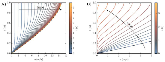
Figure 1.
Velocity profile of an infinitely long avalanche with colour marking the time. (A) Acceleration on an inclined plane. The simulation started from rest, the velocity profile tends to the Bagnold profile in steady state (black dotted line). (B) Deceleration on a flat plane. The simulation started with the steady state Bagnold profile of an inclined plane from panel A, and leads to a gradual deposition starting from the bottom.
The last transformation is conducted for the sake of similarity to the Voellmy relation [1], which is well known in the avalanche community [8]. A notable difference in comparison to the Voellmy model is the dependence on the flow thickness h in Equation (7).
A transient velocity profile for the constitutive model of Equation (5) can be derived with a numerical solution [37]. These results provide information about the flow behaviour of this constitutive model, but more importantly, allow the development of a deposition model. We model a generic solution for an avalanche with a constant height of on a plane with inclination . Material parameters have been set to and . The result is shown in Figure 1A. The avalanche starts as a plug-flow and the shear zone is initially limited to a small region near the bottom. This zone grows until the whole flow is dominated by shearing in the steady state. The steady state is reached after a few seconds in this example and the same is observed in real avalanches [38]. Therefore the steady state velocity profile together with the respective basal friction and shape factor are assumed to be a good approximation for dense snow avalanches as investigated here.
Deposition is a consequence of the avalanche decelerating, as parts of, and finally the entire avalanche, reach standstill. Up until now the deposition process has not been incorporated explicitly into snow avalanche simulations. Usually, deposition is assumed when the avalanche reaches a depth-averaged velocity of , which corresponds to an abruptly stopping block. Here, the solution for the transient velocity profile hints towards a different stopping behaviour. Considering the Bagnold profile from steady state at a slope angle of from Figure 1A, a sudden reduction of the slope angle to leads to a deceleration of the avalanche and a variation in the velocity profile as shown in Figure 1B. It can be seen that not all of the avalanche comes to standstill at the same time. Rather, the avalanche comes to standstill layer-wise starting from the bottom so that the moving mass is reduced gradually. The stopped, that is, deposited volume, expressed by the height where , is shown as a function of the depth-integrated momentum in Figure 2 together with the velocity profiles of the moving layer. This behaviour has to be modelled within the depth-integrated framework by expressing the flux from the moving to the static layer, that is, the vertical velocity of the highest point where .
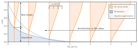
Figure 2.
The deposition depth as a function of the depth-integrated momentum from granular simulations (not depth-averaged). The respective velocity profiles during deceleration on a flat plane for each given momentum are shown in orange. The dashed line shows the behaviour of the relation for the depth-integrated model derived in Equation (10).
The temporal change in the depth-integrated momentum can be attributed to two contributions, a reduction of the depth-averaged velocity and the loss of mass , expressed by the product rule,
We split this equation using an arbitrary parameter into
The term is the deposition rate, defining the form of such a relation in a depth-integrated framework,
The parameter a can now be prescribed in such a way that the decisive behaviour of three-dimensional simulations is retained in the depth-integrated flow model. From Figure 2 we can deduce that no mass is deposited above a certain depth-averaged velocity, , approximately in the presented example, therefore for . Below this critical velocity, the deposition rate increases with decreasing velocity. When the depth-averaged velocity approaches zero, all mass will be deposited, therefore for . This behaviour can be approximated with a linear dependence on the depth-averaged velocity,
The second condition in Equation (11) ensures that the deposition model is only active during deceleration. The critical deposition velocity acts as an empirical parameter to calibrate the model to snow avalanche data. Further improvements are possible by fine tuning the relation in Equation (11), for example, with a polynomial function, but it does not seem necessary yet, considering the large uncertainties involved.
The simplified deposition model can be evaluated with a simple block model on a flat plane. We use the basal friction model to calculate the deceleration of the block and further the resulting deposition. This depth-integrated solution is included in Figure 2 as the blue-dashed line for comparison with the full numerical solution. The simple model captures the behaviour of the complex model reasonably well, with some limitations.
To implement this approach into the depth-integrated flow model, the total temporal derivative of the depth-integrated momentum in flow direction is calculated as
and incorporated in Equation (10).
The entrainment flux is the last term that needs to be described. Without doubt, entrainment of resting snow into the flowing avalanche has a large influence on the flow dynamics [17], and entrainment models are nowadays included in most simulation tools. A gradual entrainment model, as applied by Fischer et al. [26] and Rauter et al. [31], is applied in this work,
The parameter represents the erosion energy and defines the erosion speed, which is usually determined by experimental data [26]. Note that this model predicts an enormous and unrealistic growth of the entrainment rate for high velocity flows. However, entrainment is limited by the available snow cover , which prevents unrealistic entrainment.
The final model used for simulations is composed of the balance equations for flowing mass Equation (1) and resting mass Equation (2), surface tangential momentum Equation (3) and surface normal momentum Equation (4). The basal friction model Equation (7), the entrainment model Equation (13) and the deposition model Equation (10) close the system. The numerical routine is based on the Finite Area Method which is implemented into OpenFOAM [39,40] and described in detail by Rauter and Tuković [33]. Further practical aspects, such as the interaction with GIS, are covered by Rauter et al. [32].
2.2. Experimental Avalanche Data
Extensive full-scale avalanche experiments are performed at the Vallée de la Sionne test site in Switzerland since 1997 [27]. The test site consists of an east-facing slope with several release areas spread over a width of 1500 m and overall track length of approximately 3000 m (Figure 3). While the release area between 2350–2700 m above sea level (asl) has a slope angle of to , the runout zone below 1800 m asl flattens towards approximately . The valley floor is found at about 1400 m asl, giving an overall drop height from release area to runout zone of 1300 m. The test site provides a large range of flow data, captured by sensors spread over the whole mountain slope. Sensors with direct flow contact are mounted on a tall steel pylon in the middle of the avalanche track at 1650 m asl, and remote sensing devices are housed in a bunker (1450 m asl) on the counter-slope 50 m above the valley floor at 1400 m asl [27].
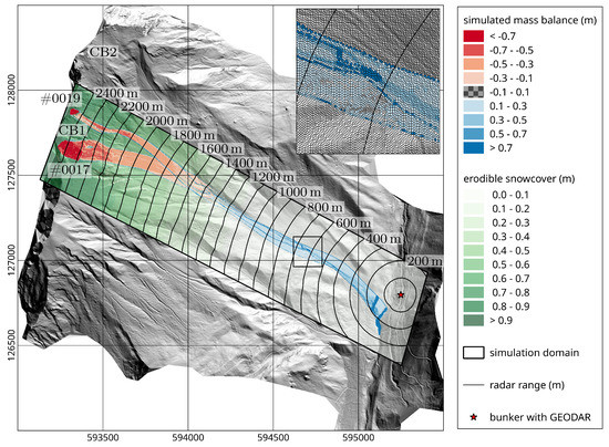
Figure 3.
Overview of the avalanche test site Vallée de la Sionne (VdlS) with both simulated avalanches (#0017 lower release area, #0019 above) from release areas Crêta Besse (CB1/2). The simulated mass balance summarizing entrainment (red) and deposition (blue) of the two consecutive avalanches is shown, together with the entrainable snow cover (green) that linearly increases from 0–1 m above 1200 m range until the mountain top. Black contour lines indicate the radar range (distance from GEODAR in the valley floor). The area in the black square is zoomed in the upper right corner showing the computational mesh and the deposition patterns of both avalanches with the dark blue area corresponding to the runout of avalanche #0019. Coordinates are given the Swiss coordinate system CH1903 (SRID 21781).
Here we use remote sensing data from the GEODAR (GEOphysical flow dynamics using pulsed Doppler radAR) [41], which is a frequency-modulated continuous-wave radar system. The radar operates at a wavelength of , which approximately defines the minimal size of granules and snow clumps that can be seen by the radar. This means that all dense flow features are mapped, but the fine-grained powder cloud is largely transparent to the radar [19]. The radar is able to resolve mainly the range (distance from the antenna, for example, see black isolines in Figure 3), but advanced data processing can yield a Doppler velocity and a lateral position of the avalanche. The complete slope of the test site is monitored at frame rate with range (distance from radar) resolution. Moving radar targets like an avalanche can be identified by focusing on temporal changes in the radar signal with a high-pass filter known as moving target identification (MTI) [29]. Such MTI images resolve the approaching avalanche in range and in time. Examples of MTI images are shown in Figure 4 and Figure 5; the added simulation data are described in Section 3. The signal intensity is determined by the reflectance of the target (material and size) and change rate (velocity and turbulence). Since there is not yet a method to interpret this intensity quantitatively [19], we restrict ourselves to the tracking of front and tail of the avalanche, thus, tracking the lower left and upper right edge of high-intensity areas in the MTI image. The evolution of the front position with time—or the gradient of the lower left edge—yields the so-called approach velocity (see Köhler et al. [19] for an in-depth description of the MTI images). However, this approach velocity does not match the depth-integrated velocity of the flow model and therefore no direct comparison is possible. To solve this issue, we base our validation method on simulation of synthesised MTI data for direct comparison with the radar data.
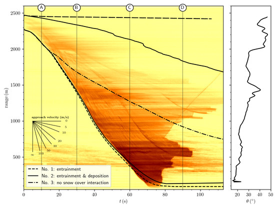
Figure 4.
Moving target identification plot of avalanche #0017. The GEODAR data are shown in the background. Black lines give the front and tail position extracted from the simulations. Material and model parameters are optimized to this avalanche. Simulation no. 1 solely includes entrainment, simulation no. 2 includes entrainment and deposition, vertical lines correspond to the snapshots (A–D) in Figure 6. Simulation no. 3 is drawn as reference without entrainment and deposition. The slope angle along the line of steepest descend is shown in the right panel. A velocity legend is included for quick translation of front inclination to approach velocity. Black lines represent the front and tail position extracted from simulations (Section 3).
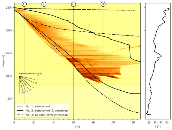
Figure 5.
Moving target identification plot of avalanche #0019. The GEODAR data are shown in the background. Black lines give the front and tail position extracted from the simulations. No optimization of parameters has been conducted for this avalanche, but material and model parameters are taken from optimization to avalanche #0017 in Figure 4. Simulation no. 1 solely includes entrainment, simulation no. 2 includes entrainment and deposition, vertical lines correspond to the snapshots (E–H) in Figure 6. Simulation no. 3 is drawn as reference without entrainment and deposition. The slope angle along the line of steepest descend is shown in the right panel. A velocity legend is included for quick translation of front inclination to approach velocity. Black lines represent the front and tail position extracted from simulations (Section 3).
In this paper we analyze two avalanches in detail, events #0017 and #0019 from 3 February 2015 that were released after a snowfall period with about of cold new snow on top of an unfavourable snow cover. The MTI data for the respective events can be retrieved from the GEODAR data repository [42]. The respective MTI images are shown in Figure 4 and Figure 5. Detailed analysis of these events with respect to the GEODAR data is reported by Köhler et al. [29].
Avalanche #0017 was released from the left side of Crêta Besse 1 and descended through channel 1 (see Figure 3). The initial release was rather small with a volume of 15,200 m but secondary slabs and entrainment led to an overall volume of 78,500 m [29], once more highlighting the importance of entrainment. At about 1800 m asl, the avalanche joined the track of a previous avalanche and encountered deposited snow rather than undisturbed snow cover. Avalanche #0017 was a typical powder snow avalanche that showed multiple minor surges as the characteristics for the intermittent frontal region, and thus was able to progress over the shallow runout zone with high velocity [22].
Avalanche #0019 was released between Crêta Besse 1 and Crêta Besse 2 and merged into the flow path of avalanche #0017 at 2100 m asl after descending 400 m. The initial release with a volume of 2200 m and the total volume of 29,500 m were smaller by a factor of 2 to 3 than avalanche #0017. The runout of avalanche #0019 was distinctly shorter, stopping in the middle of the steep track (see Figure 3). Interestingly, avalanche #0019 showed larger surges rather than minor surges. These large surges resemble dense flows that originate from the confined releases of secondary slabs [29]. This avalanche may have partly formed minor surges shortly before halting at ranges below . However, they were not able to change the flow dynamics towards a powder snow avalanche and the avalanche starved out quickly.
Both events differ substantially in size and flow patterns, but they were released within a short interval so that the snow conditions were essentially the same. Avalanche #0017 is classified as large according to its runout, avalanche #0019 as medium-size; it stopped in steep terrain [43]. We aim to simulate these two events with the same set of parameters as this would indicate a physical meaning of the parameters.
3. Simulation Setup and Results
The model requires several parameters, boundary and initial conditions to successfully simulate the flow of an avalanche. Namely, the terrain as a surface mesh, the initial erodible snow cover, the release area and the four model parameters , , and are required.
The surface mesh for the simulation was generated based on a digital elevation model (DEM), which had been acquired by an airborne laser scan during summer when the slope was free of snow. The mesh generation follows the scheme presented by Rauter et al. [32] and is based on the library cfMesh [44]. The DEM gets slightly smoothed by the meshing routine, however, in reality terrain roughness gets lowered by the snow cover as well. A simulation covering of real time for the domain shown in Figure 3 (291,207 cells with an average size of covering an area of approximately ) takes about on 4 cores of an Intel i-7700K. We chose the first-order upwind Gauss scheme for convective terms and the linear Gauss scheme for other spatial derivatives, time integration is performed using an implicit second-order accurate scheme and non-linear systems were solved to a relative residuum of .
The initial mountain snow cover represents the erodible snow cover. We estimate the amount with the local meteorological and nivological conditions during 3 February 2015. We assume that only the preceding snowfall of about contributed to the avalanches. Furthermore, an earlier avalanche on the same day cleared all snow from the lower part of the track, so that no significant erodible layer exists below 1800 m asl (or 1200 m radar range). As with previous work [26,31], we assume a linear snow height distribution with elevation, giving a snow height of 1 m at 2500 m asl that decreases about 1.4 mm every meter and results in no erodible snow below 1800 m asl as shown in Figure 3.
The release areas for avalanche #0017 and #0019 are taken from Köhler et al. [29], matching the estimated release volumes. The initial snow cover height for simulation #0019 is set to the snow cover height of the last time step of simulation #0017. This way, avalanche #0019 cannot entrain snow that has already been taken by the preceding avalanche #0017 and we are able to simulate the chain of events on this day.
Simulation quality and optimal model parameters are found by comparing the front and tail positions between simulation and experiment. Rather than extracting this position from the radar and transforming the range into real world coordinates, we choose to emulate the GEODAR data within the simulation and thus produce synthetic MTI range-time plots to be directly comparable with the radar data (see Videos S1 and S2 in supplementary materials). Here, the exact intensity or colouring of the MTI images is not important as we are only interested in the position of front and tail. For now, we chose the surface integral of depth-averaged velocity as the simulated intensity. Although this quantity is not related to the GEODAR signal, it gives a good contrast in simulated MTIs, well suited to identify front and tail. The contribution of a finite area cell P to intensity, calculated as the product of depth-averaged velocity and cell area , is assigned to a specific range gate by calculating and classifying the distance between cell centre and virtual radar position. Here, we use 260 range gates with a distance between range gates of 10 m, defining the spatial resolution of the synthetic MTI plots. This process is conducted 20 times per second, defining the temporal resolution. Finally, the front and tail positions are found as the closest and farthest ranges where a specific threshold in intensity is exceeded. The method is insensitive to the exact threshold, at least for the chosen formulation of simulated intensity. Front and tail positions from experiment and simulation can then be compared to get a criterion for the fitness of simulations.
The shape factor is set to following the Bagnold velocity profile and has not been optimized for the experimental data. This choice is consistent with the friction model Equation (5).
Parameters , , and have been fitted to the simulations. Generally speaking, each parameter has a characteristic influence on the avalanche kinematics. The dry friction parameter is the key to matching the runout, that is, the farthest point of the avalanche. The turbulent friction parameter can be estimated by matching the approach velocity in steady state, that is, the maximum inclination of the front in the MTI-plot. The specific entrainment energy allows to balance the velocity in the release area with the velocity in the runout zone and the growth rate of the avalanche in terms of mass and volume. The deposition parameter can be chosen so that the tail of the avalanche shows realistic extensions. Although all parameters influence all kinematic characteristics to some extent, these leading-order effects allow us to manually find the appropriate model parameters. As mentioned before, we aim to simulate the two consecutive avalanches with the same set of parameters. We chose to find optimized parameters for #0017 and apply them to #0019. In future work, automatic optimization methods as shown by Fischer et al. [26] and Rauter et al. [31] should be applied. We finally find the optimum parameters as displayed in Table 1.

Table 1.
Summary of simulation parameters for both consecutive avalanches #0017 and #0019. , and are determined with simulation no. 1 on avalanche #0017, resulted from simulation no. 2 on the same avalanche.
In order to disentangle the effects of entrainment and deposition, we ran multiple setups, including or excluding respective processes. Simulation setup no. 1 includes entrainment of the available snow cover shown in Figure 3, but deposition is turned off. This roughly resembles the classic model as used in practice today, for example, References [8,26,32], but note the slightly different friction model. Optimal parameters for this setup and avalanche #0017 (Table 1) are found by matching the dashed front line with the experimental data in the range-time MTI diagram of Figure 4. The runout and the approach velocity can be matched successfully; however, the tail cannot be simulated satisfactorily by this setup. In contrast to observations, the tail never deposits but rather continuously creeps down along the steep upper slope. This simulation setup shows a serious discrepancy regarding avalanche #0019 (Figure 5), as the simulation predicts runout to the valley floor. The issue of the constantly moving tail persists in this simulation as well, indicating the need for a deposition model.
Simulation setup no. 2 adds the newly introduced deposition model to the previous simulation setup no. 1. The deposition velocity is optimized to reproduce the shape of tail of #0017 at ranges above (Figure 4). Parameters , and are taken from setup no. 1. This approach has been chosen as the deposition model should have no leading-order effect on the approach velocity, which was used to calibrate all other parameters. Note, we focus only on the front and tail position of the avalanche, but neglect any stopping behaviour between the front and tail line in the MTI image, because the assumption of a cohesionless granular material may not hold there [19]. We found an optimum value of , which is in reasonable agreement with the value predicted from three-dimensional simulations (Figure 2). The simulation of avalanche #0019 improves significantly with the deposition model and enables the simulated avalanche to stop in steep terrain (black line in Figure 5). Snapshots at four time steps of simulation setup no. 2 are shown in Figure 6 for avalanche #0017 (A–D) and #0019 (E–H). The flowing area of the avalanche is coloured with the depth-averaged velocity , which is for #0019 approximately half of the maximum speed of #0017. Note that the depth-averaged velocity differs notably from the approach velocity that can be derived from the range-time diagrams in Figure 4 and Figure 5. Roughly speaking, the approach velocity is about higher than the depth-averaged velocity, partially due to a non-uniform velocity profile. Animations of simulations with setup no. 2 for avalanches #0017 and #0019 are provided in the supplementary materials as Videos S1 and S2.
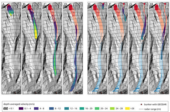
Figure 6.
Time series of the simulation for avalanche #0017 (A–D) and #0019 (E–H) at 10, 30, 60 and . Concentric circles mark the line-of-sight distance from the bunker giving the radar range. The flowing avalanche is indicated with the depth-averaged velocity . In the background, snow cover changes due to entrainment (red) and deposition (blue) are indicated with the same colour scale as the simulated mass balance in Figure 3.
Simulation setup no. 3, ignoring any interaction with the snow cover, shows drastic effects of neglecting entrainment and also deposition in avalanche simulations, as observed by others as well [30]. Large differences between experimental radar data and simulation for the front, tail and the runout are found using the model parameters and from simulation setup no. 1 (see dash-dotted lines in Figure 4 and Figure 5), however, which was expected.
4. Discussion
The aim of this study is to simulate multiple avalanches with a single set of parameters. This strategy differs from the current practice. For prediction, simple rules are applied to alter model parameters based on terrain shape and avalanche size [2]. For back-calculation of past events the parameters are found by optimizing the simulation results to empirical data. However, varying material parameters to cover size and flow regime effects is not desired and reflects our poor understanding of these phenomena. We argue that these effects should be resolved by the model, provided that it captures all relevant physical processes.
Simulation setup no. 1 represents a common setup including a simple friction model and entrainment (except for the shape factor). From a practical perspective, simulation setup no. 1 seems acceptable for avalanche #0017 as runout and front velocity match surprisingly well. These are indicators for the reach and destructive potential and as such the most important results. The poorly represented tail is of minor importance for hazard zone mapping, as no destructive potential is associated with it. However, applying the parameters optimized for avalanche #0017 to avalanche #0019, the dashed line in Figure 5 reveals large discrepancies in terms of runout, which is a problem of practical relevance. Overestimation of small avalanches has been observed in simulations before and poses a problem in describing these events. This issue is usually addressed with larger values for smaller avalanches [2].
Adding the novel deposition model in simulation setup no. 2 allows to simulate both avalanches to higher accuracy. Improvements for avalanche #0017 are mostly the shorter tail, whereas the front behaves similar to simulation setup no. 1. Bigger influences of the deposition model are found for avalanche #0019, which now stops after the steep couloir at the beginning of the runout area where the slope is about . This was not possible in setup no. 1, as this model lacks the ability for stopping and deposition, except on slopes flatter than the friction angle. Since the chosen friction coefficient corresponds to a friction angle of , no stopping is possible on steeper slopes with simulation setup no. 1.
Both simulation setups, no. 1 and no. 2, show a high sensitivity to the slope angle and the velocity reduces consistently in the transition phase between the steep avalanche track and the flat runout zone. However, such behaviour cannot be observed in the radar data for avalanche #0017 or other powder snow avalanches [19]. In contrast, powder snow avalanches keep their speed when transitioning from a steep to more gently inclined slope. We attribute this mismatch to the missing intermittent [22] or fluidized [15] flow regime in our dense flow model.
Avalanche #0019 shows an abrupt increase in the approach velocity at range 1300 m. This knick is clearly visible in the radar data, as well as in both simulation setups and shows the ability of the OpenFOAM solver to accurately capture complex natural terrain. Even though the initial acceleration for #0019 is underestimated by both simulation setups, causing the small splitting of experiment and simulation, the overall approach velocity or gradient of the front after is comparable in the range-time diagram.
The optimized dry friction coefficient and the turbulent friction coefficient = 6000 m s are very similar to previous optimization studies [31]. Note that the deposition model works best with reasonable turbulent friction and a respective parameter , as this increases effective friction in shallow parts of the avalanche and leads to a stronger deposition at the tale and sides.
Obviously, simulation setup no. 3 without entrainment and deposition, is dominated by the lack of mobilized mass, because the initial volume is only 10–20% of the reported total mobilized volume for either avalanche (Figure 7). Effects on the initial acceleration are rather marginal, but larger deviations in velocity and runout occur in the lower part of the track. There is no set of parameters for this setup that can adjust the velocity in the lower parts without worsening results in the upper part. This is consistent with the assumed effect of entrainment—little influence during the initial phase but high influence in the lower part, where vast amounts of snow could be accumulated due to entrainment. This emphasizes the need for explicit entrainment modelling in simulations for hazard mitigation measures.
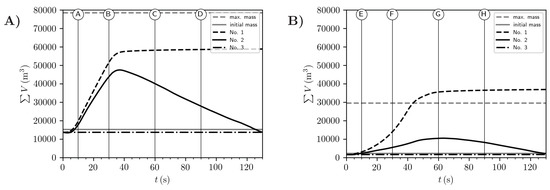
Figure 7.
The sum of the mobilized volume in the simulation for (A) avalanche #0017 and (B) avalanche #0019 for the three simulation setups no. 1, no. 2 and no. 3. The vertical markers A–D and E–H correspond to the snapshots of the simulations in Figure 6 and the markers in the MTI images (Figure 4 and Figure 5). Gray horizontal lines give volumes of initial release (lower line) and total volume (upper line), reported by Köhler et al. [29].
The setup no. 1, representing a commonly applied model, implements the mass growth of avalanches and the mobilized mass increases monotonically from release until the end of the simulation. The deposition model in setup no. 2 allows a more realistic behaviour. The mobilized mass now shows a peak after an initial increase due to entrainment followed by a decrease due to deposition (Figure 7). Note, the reported total volumes are upper thresholds since mass flows will never include the total mobilized mass at a single moment. The mobilized volumes depend heavily on the available snow cover. In fact, we manage entrainment mainly with a smart distribution of available snow cover. This is a strong simplification of the complex snow distribution on that day (preceding avalanches, old depositions, warm and compact snow in lower parts) and more sophisticated methods are desirable. However, we are convinced that we were able to reproduce the significant conditions for avalanche #0017, namely high amounts of fresh snow at altitudes above 1800 m asl and no erodible snow cover below. In reality, the deposits in the lower part of a preceding avalanche (#0016) are likely to be entrained partly by #0017 and #0019. However, we neglect this here, since the compact deposits may withstand high shear stresses, effectively resisting entrainment. In conclusion we would like to emphasize the need for improved and physically based entrainment models, considering the effect of snow cover properties.
A major novelty of this work is the deposition model within the depth-averaged simulation framework. The development has been inspired and made possible by the high-resolution radar data that show the important role of deposition at the tail. In operational snow avalanche modelling, it is common to artificially threshold the simulation durations and the final timestep is interpreted as deposition [8]. The deposition model provides the advantage of stopping the avalanche based on a physically motivated concept. We want to note that the proposed two-layer methodology is not unique in being able to produce respective entrainment-deposition patterns. Edwards et al. [45,46] and Rocha et al. [47] successfully apply a depth-integrated single-layer model with a frictional hysteresis for the simulation of entrainment-deposition patterns and levees in small-scale experiments.
Köhler et al. [19] analysed the stopping of avalanches and found four stopping mechanisms, three of which could be linked to the snow properties along the avalanche track. However, the presented deposition model represents solely two of the four mechanisms, that is, tail deposition and starving. Aside from these mechanisms that correspond to dry cohesionless granular flow, we can observe abrupt stopping and backward propagating shocks in radar MTI plots [19]. None of these were accounted for in this work, as this would require modelling of respective flow regimes (wet snow) prior to that. Abrupt stopping must be related to a plug profile which contradicts the assumed rheology. The same can be said for backward propagating shocks, which cannot be covered by the simple local considerations of the deposition model. To model a backward propagating shock it might be sufficient to include the influence of the deposition pattern on the movement, for example, to add the deposition heights to topography. This should introduce further resistance to the flowing mass and enable deposition starting from a stopping front. Moreover, thermodynamic effects are expected to play a major role in the stopping behaviour. Wet snow changes its rheology from a frictional towards a cohesive or plastic regime, allowing plug flows and thus transition from starving to abrupt stopping mechanisms.
Our deposition model requires a critical deposition velocity as input parameter, which we found to be reasonable in the range of . This means that as soon as the depth-averaged velocity falls below this value, some snow is removed from the flowing avalanche. This parametrisation approximates the behaviour known from full 3D simulation of granular flows [37] during deceleration. In combination with an increased friction in shallow areas, the model mimics the tendency to levee formation, known from granular experiments [47]. Furthermore, the deposition model leads to a spread of deposited mass over the whole avalanche path, including areas steeper than the friction angle. To which extent this compares to real deposits of dense snow avalanches is still unclear, but should be investigated in future studies. Methodically, this should follow the experimental approach of Sovilla et al. [48], who find a gradual increase of deposit heights with decrease of slope angle. Since the avalanche velocity that mainly controls deposition is highly dependent on the slope angle, we expect a reasonable match with data and a valuable test of the deposition model.
Even though the runout in simulation no. 2 of #0019 is overestimated by approximately range, the powerful part of the avalanche stops at a similar point as radar measurements indicate and solely a narrow, shallow and slow slide remains (compare time step H in Figure 5 and Figure 6). The stopping in the simulation is related to topographic features, that is, the start of the runout area and the end of the confined couloir, but old deposits having higher roughness and shear strength will in reality also contribute. The deposits of avalanche #0017 (and #0016) may have played an important role for avalanche #0019, increasing the roughness of the base substantially and causing the avalanche to stop earlier. However, such details are hard to include in a systematic way which can be used in real-world applications. The simulated tail of #0019 matches the measurement equally well as in simulation #0017. This indicates that the deposition model captures a physical process that consistently appears in snow avalanches of different size and type.
A usable deposition model might be of high relevance for practitioners, as it allows consideration of accurate deposition patterns and mass distributions during assessment of risks and planning of protection measures. As directly shown here, when several consecutive avalanches are simulated, one can maintain a realistic snow cover for later events. The enhanced estimation of mass transports and their spatial distribution can help to improve design and dimensioning of defence structures like catchment dams. However, such examples of advanced usage require further research and validation of mass fluxes and depositions.
Interestingly, a tendency to produce levees can be observed in the model results, especially in the lower but also in the upper parts of the track. They are produced by the interaction between high friction at small flow heights, for example, at lateral edges of the avalanche, and the deposition model. The high effective friction leads to velocities below the deposition velocity which activates the deposition model. This initiates a positive feedback of reduced flow height, increased friction and deposition. We also observed that the width of levees extends solely over one to three cells and 2–7 m respectively (see zoom in Figure 3). Although this is a realistic width for levees in snow avalanches, we may have encountered a grid-dependent effect. At the current point we are not able to validate the position nor the form of the generated levees, but a separate study should make a conclusive assessment. Moreover, the current implementation neglects the influence of deposition patterns on the topography over which the avalanche flows and guiding effects of deposition and levees are ignored by the model. These aspects should be elaborated in the future, investigating the effect of levees and other deposition patterns on flow dynamics.
The shape factor of is consistent with the Bagnold velocity profile and granular rheology. The majority of studies neglect the shape factor due to numerical instabilities [49] and a lack of need. A shape factor larger than unity increases mass transport in the direction of motion and thus stretches the avalanche and increases approach velocities. However, we observed that in practice the shape factor has a rather small influence on the approach velocity. As the avalanche spreads out, effective friction increases and the velocity is decreased. The approach velocity is slightly higher with the higher shape factor. Moreover, the lateral extension is reduced by a larger shape factor. As a consequence, the path where the avalanche is able to entrain snow is narrower and the overall mobilized mass lower.
Interestingly, simulations with show the tendencies to produce wave-like instabilities in situations without entrainment. This behaviour can be explained by the rheological model and is commonly observed [50]. We find that the classic Voellmy model does not tend to produce these instabilities. However, the shape factor of , pulls the wave-like structures apart, effectively eliminating these waves. It remains an interesting task to investigate which rheological and flow model produces these instabilities and whether they are connected to surges as observed in snow avalanches.
The model is based on assumptions that fit solely to a dense snow avalanche, the intermittent or fluidized regime is not included in the model. Therefore the simulation falls behind the real avalanche in terms of approach velocity as avalanche #0017 reaches the gentle slope in the deposition area earlier. The real avalanche is able to maintain its velocity due to fluidization [29], while the simulated avalanche switches into a new steady state with reduced velocity. This appears as a bend in the front position below range of the simulated avalanche while the measurement forms an almost straight line in the MTI plot of Figure 4. Some suggestions that include such a fluidized flow regime exist in the literature [15,25].
Köhler et al. [29] present avalanches #0017 and #0019 as examples of two different surges in avalanches. Here, we simulate them with a model not capable of reproducing surges at all. The minor surges seen in avalanche #0017 are direct indicators for the formation of the above mentioned intermittent flow regime. However, the major surges which define #0019 originate from isolated slab releases. It is theoretically feasible to simulate them directly by explicitly defining their extent and release timing in the model. Such confined releases cause surges to flow independently of each other and eventually overtake each other, causing bends and kinks in the front. However, slab releases make any prediction of avalanches much more complicated and it would be nearly impossible to predict locations and extent of secondary slabs prior to an event. We see in the good match of experiment and simulation that considering the overall mass growth with continuous entrainment might be sufficient for an overall picture (say average approach velocity and runout) of the avalanche. Possibly, the influence of slabs on simulations is not as important as other factors like thermodynamics and flow regime transitions.
MTI images or in general range-time diagrams are an intuitive way to present simulation results and give good temporal overview, rather than spatial maps that present discrete time stamps, that is, Figure 6. The direct comparison of measurements with synthetic data has some key advantages. The radar data processing is held to a minimum, as no geometric conversions onto the terrain nor any derivation of velocity is needed. Comparing the position with time is an obvious quantity, well defined in both, measurement and simulation. The difference between measurement and simulation in a range-time diagram can furthermore be directly used to define a numerical fitness parameter which can be used in automatic optimisation procedures.
Even though comparing front and tail positions gives unprecedented validation, we still miss important quantities, that is, everything happening in the avalanche body. However, it is challenging to estimate flow features from the measured MTI intensity and vice versa to generate sensible MTI intensities from simulations. For example, we cannot extract particle velocities, entrainment and deposition fluxes or mass from radar data, but we need to infer their effect on front and tail. At the same time, it is unclear how to synthesize MTI intensity in simulations such that it is quantitatively comparable to respective radar intensities. We hope to be able to generate meaningful MTI intensities based on simulated flow fields (velocity, turbulent kinetic energy, flow height) in the future. This should not only improve comparison strategies but also increase the knowledge drawn from radar measurements, using a model-based data interpretation scheme.
The validation with the high-resolution radar is very challenging for current models. We expect that a new generation of models will be required and inspired by challenges like this. The deposition model presented here should be seen as an example for an improvement that has been inspired by the high-quality data and enhances the model results to some extent.
Our comparison strategy between measurements and simulations should be generalized in the future. Rather than transforming measurements for comparison with simulation outputs, we propose to synthesise data to compare it directly with measurements. Our method to match simulations with the range-time representation of GEODAR data is still very simple. One can imagine more complex routines that take physical backscatter and propagation of microwaves into account to resemble the MTI intensities. However, such an approach might be very complex and more care needs to be taken to match the physical constraints of the measurement device. Other sensible measurements that should be interpreted with such a direct data synthetisation are for example mass balance data from laser scan measurements, velocity histograms to be compared with Doppler radar [28], vertical flow profiling radars [17] and seismic ground-movements [51]. Synthesising measurement data usually requires deep access to the internals of the model code; however, it will make the data comparison task tremendously simpler in most cases. Here, OpenFOAM provides as a strong platform to easily implement data synthesising modules and new models. The model solver and the respective tools are available within the avalanche module of OpenFOAM and can be freely modified, advanced and redistributed.
5. Conclusions
We challenge a depth-integrated avalanche model with the simulation of a chain of avalanche events, that has been recorded by the high-resolution GEODAR radar. By developing and adding a deposition model, the simulation results are in satisfactory agreement with observations, considering the simplicity of the flow model. The results show once more that depth-integrated models and the respective tools can provide useful information for hazard estimation and mitigation planning. However, the detailed analysis of the simulations and the comparison with high-resolution radar data reveal issues and the need for further improvement.
We introduced a simple deposition model, inspired by a dry granular flow model. The inclusion of deposition processes are the consequent evolution of entrainment models, completing the mass exchange cycle with the snow cover. This improves the model performance regarding the tail of the avalanche and deposition patterns. Moreover, starving avalanches in steep slopes with inclinations bigger than the friction angle can be successfully explained by the modified model.
The model has been validated using a detailed analysis of two consecutive avalanches. A comparison based on the high resolution GEODAR showed remarkable agreement for some flow features but also revealed some important issues that have to be faced in the future. The GEODAR data and other direct measurements in avalanches give us a new understanding of flow regimes and provide a great opportunity for further model development, calibration and validation. It will be the crucial task of the next generation of mass flow models to consider these regimes and the respective regime changes. Besides the validation of the Finite Area Method for snow avalanches, this work provides a valuable benchmark for those future developments.
Furthermore, we see great demand concerning improved and physically based entrainment models. In this work we controlled entrainment by carefully modelling the erodible mountain snow cover. A high degree of expert judgement was involved in this procedure. More sophisticated approaches are required to streamline this process and to put it on a more objective level, as well as consider the effects of different snow properties like old compacted deposits.
The deposition model introduces important effects into the simulation, improving especially the simulation of the mid-sized avalanche #0019. We see a great opportunity for the deposition model to improve the calculation of mass balances and for example the design of catchment dams. Moreover, the generation and the effect of levees can be studied with this model. This will require considerable validation that cannot be achieved with the GEODAR data alone. Here, small-scale experiments and laserscan recordings of the net mass balance of the avalanche are certainly more appropriate.
OpenFOAM proves to be a powerful platform for model evaluation and development. The emulation of the radar signal is a simple extension to the existing OpenFOAM solver and a wide range of improvements are possible. Previous comparison techniques struggled when comparing simulations with measurements due to the rigid and closed structure of the simulation tools. The open structure of OpenFOAM enabled us to rapidly implement deposition as an extension to the classic model. We look forward to implementations of more processes to further improve simulations based on the presented benchmark.
Finally, we want to note that all developments are freely available for interested users. The open structure invites users to evaluate their own ideas and makes these developments applicable to real cases. It is uncertain how future avalanche models will look, but certainly they will require open-source frameworks like OpenFOAM and benchmarks like GEODAR.
Supplementary Materials
The following are available at https://www.mdpi.com/2076-3263/10/1/9/s1, Video S1: Simulation of avalanche #0017. Video S2: Simulation of avalanche #0019.
Author Contributions
M.R. contributed the model development. A.K. contributed to data acquisition and interpretation. Both authors contributed to the formal analysis, the interpretation and the writing. All authors have read and agreed to the published version of the manuscript.
Funding
M.R. received funding from the Austrian Academy of Sciences (OEAW) project “beyond dense flow avalanches” and the European Union’s Horizon 2020 research and innovation programme under the Marie Skłodowska-Curie grant agreement No. 721403 (SLATE). A.K. received funding from the Swiss National Science Foundation (SNSF) projects “High Resolution Radar Imaging of Snow Avalanches” (200021_143435) and “Identify critical terrain features and flow states on surge formation in snow avalanches” (P400P2_186687).
Acknowledgments
The presented computational results have been achieved (in part) using the HPC infrastructure LEO of the University of Innsbruck. For the experimental avalanche data, we thank the SLF for operating the avalanche test-site. M.R. gratefully acknowledges the scientific support by Wolfgang Fellin and Jan-Thomas Fischer. A.K. thanks Betty Sovilla and Jim McElwaine. We thank Dieter Issler, Chris Johnson, Julia Kowalski and 2 anonymous referees for a careful reading of the manuscript and many helpful comments.
Conflicts of Interest
The authors declare no conflict of interest. The funders had no role in the design of the study; in the collection, analyses, or interpretation of data; in the writing of the manuscript, or in the decision to publish the results.
References
- Voellmy, A. Über die Zerstörungskraft von Lawinen (On the destructive forces of avalanches). Schweizerische Bauzeitung 1955, 73, 159–165. [Google Scholar] [CrossRef]
- Gruber, U.; Bartelt, P. Snow avalanche hazard modelling of large areas using shallow water numerical methods and GIS. Environ. Model. Softw. 2007, 22, 1472–1481. [Google Scholar] [CrossRef]
- Grigorian, S.S.; Eglit, M.E.; Iakimov, Y.L. A new formulation and solution of the problem of snow avalanche motion. Trudy Vysokogornogo Geofizicheskogo Instituta 1967, 12, 104–113. [Google Scholar]
- Savage, S.B.; Hutter, K. The motion of a finite mass of granular material down a rough incline. J. Fluid Mech. 1989, 199, 177–215. [Google Scholar] [CrossRef]
- Savage, S.B.; Hutter, K. The dynamics of avalanches of granular materials from initiation to runout. Part I: Analysis. Acta Mech. 1991, 86, 201–223. [Google Scholar] [CrossRef]
- Pitman, E.B.; Nichita, C.C.; Patra, A.; Bauer, A.; Sheridan, M.; Bursik, M. Computing granular avalanches and landslides. Phys. Fluids 2003, 15, 3638–3646. [Google Scholar] [CrossRef]
- Sampl, P.; Zwinger, T. Avalanche simulation with SAMOS. Ann. Glaciol. 2004, 38, 393–398. [Google Scholar] [CrossRef]
- Christen, M.; Kowalski, J.; Bartelt, P. RAMMS: Numerical simulation of dense snow avalanches in three-dimensional terrain. Cold Reg. Sci. Technol. 2010, 63, 1–14. [Google Scholar] [CrossRef]
- Mergili, M.; Schratz, K.; Ostermann, A.; Fellin, W. Physically-based modelling of granular flows with Open Source GIS. Nat. Haz. Earth Syst. Sci. 2012, 12, 187–200. [Google Scholar] [CrossRef]
- Ancey, C.; Bakkehøi, S.; Hutter, K.; Issler, D.; Jóhannesson, T.; Lied, K.; Nishimura, K.; Pudasaini, S. Some notes on the history of snow and avalanche research in Europe, Asia and America. Ice News Bull. Int. Glaciol. Soc. 2005, 139, 3–11. [Google Scholar]
- Gray, J.M.N.T.; Wieland, M.; Hutter, K. Gravity-driven free surface flow of granular avalanches over complex basal topography. Proc. R. Soc. Lond. Ser. A 1999, 455, 1841–1874. [Google Scholar] [CrossRef]
- Bouchut, F.; Westdickenberg, M. Gravity driven shallow water models for arbitrary topography. Commun. Math. Sci. 2004, 2, 359–389. [Google Scholar] [CrossRef]
- Denlinger, R.P.; Iverson, R.M. Granular avalanches across irregular three-dimensional terrain: 1. Theory and computation. J. Geophys. Res. 2004, 109, F01014. [Google Scholar] [CrossRef]
- Pouliquen, O.; Forterre, Y. Friction law for dense granular flows: application to the motion of a mass down a rough inclined plane. J. Fluid Mech. 2002, 453, 133–151. [Google Scholar] [CrossRef]
- Issler, D.; Gauer, P. Exploring the significance of the fluidized flow regime for avalanche hazard mapping. Ann. Glaciol. 2008, 49, 193–198. [Google Scholar] [CrossRef]
- Buser, O.; Bartelt, P. Production and decay of random kinetic energy in granular snow avalanches. J. Glaciol. 2009, 55, 3–12. [Google Scholar] [CrossRef]
- Sovilla, B.; Burlando, P.; Bartelt, P. Field experiments and numerical modeling of mass entrainment in snow avalanches. J. Geophys. Res. 2006, 111. [Google Scholar] [CrossRef]
- Sailer, R.; Fellin, W.; Fromm, R.; Jörg, P.; Rammer, L.; Sampl, P.; Schaffhauser, A. Snow avalanche mass-balance calculation and simulation-model verification. Ann. Glaciol. 2008, 48, 183–192. [Google Scholar] [CrossRef]
- Köhler, A.; McElwaine, J.N.; Sovilla, B. GEODAR data and the flow regimes of snow avalanches. J. Geophys. Res. 2018, 123. [Google Scholar] [CrossRef]
- Steinkogler, W.; Gaume, J.; Löwe, H.; Sovilla, B.; Lehning, M. Granulation of snow: From tumbler experiments to discrete element simulations. J. Geophys. Res. 2015, 120, 1107–1126. [Google Scholar] [CrossRef]
- Steinkogler, W.; Sovilla, B.; Lehning, M. Thermal energy in dry snow avalanches. Cryosphere 2015, 9, 1819–1830. [Google Scholar] [CrossRef]
- Sovilla, B.; McElwaine, J.N.; Köhler, A. The intermittency region of powder snow avalanches. J. Geophys. Res. 2018, 123, 2525–2545. [Google Scholar] [CrossRef]
- Sovilla, B.; McElwaine, J.N.; Louge, M.Y. The structure of powder snow avalanches. C. R. Phys. 2015, 16, 97–104. [Google Scholar] [CrossRef]
- Vera Valero, C.; Wikstroem Jones, K.; Bühler, Y.; Bartelt, P. Release temperature, snow-cover entrainment and the thermal flow regime of snow avalanches. J. Glaciol. 2015, 61, 173–184. [Google Scholar] [CrossRef]
- Bartelt, P.; Buser, O.; Vera Valero, C.; Bühler, Y. Configurational energy and the formation of mixed flowing/powder snow and ice avalanches. Ann. Glaciol. 2016, 57, 179–188. [Google Scholar] [CrossRef]
- Fischer, J.T.; Kofler, A.; Wolfgang, F.; Granig, M.; Kleemayr, K. Multivariate parameter optimization for computational snow avalanche simulation in 3d terrain. J. Glaciol. 2015, 875–888. [Google Scholar] [CrossRef]
- Sovilla, B.; McElwaine, J.; Steinkogler, W.; Hiller, M.; Dufour, F.; Suriñach, E.; Pérez-Guillén, C.; Fischer, J.T.; Thibert, E.; Baroudi, D. The Full-Scale Avalanche Dynamics Test Site Vallée de la Sionne; International Snow Science Workshop: Grenoble–Chamonix, France, 2013; pp. 1350–1357. [Google Scholar]
- Gauer, P.; Kern, M.; Kristensen, K.; Lied, K.; Rammer, L.; Schreiber, H. On pulsed Doppler radar measurements of avalanches and their implication to avalanche dynamics. Cold Reg. Sci. Tech. 2007, 50, 55–71. [Google Scholar] [CrossRef]
- Köhler, A.; McElwaine, J.; Sovilla, B.; Ash, M.; Brennan, P. The dynamics of surges in the 3 February 2015 avalanches in Vallée de la Sionne. J. Geophys. Res. Surf. 2016, 121, 2192–2210. [Google Scholar] [CrossRef]
- Fischer, J.T.; Fromm, R.; Gauer, P.; Sovilla, B. Evaluation of proabilistic snow avalanche simulation ensembles with Doppler radar observations. Cold Reg. Sci. Technol. 2014, 97, 151–158. [Google Scholar] [CrossRef]
- Rauter, M.; Fischer, J.T.; Fellin, W.; Kofler, A. Snow avalanche friction relation based on extended kinetic theory. Nat. Haz. Earth Syst. Sci. 2016, 16, 2325–2345. [Google Scholar] [CrossRef]
- Rauter, M.; Kofler, A.; Huber, A.; Fellin, W. faSavageHutterFOAM 1.0: depth-integrated simulation of dense snow avalanches on natural terrain with OpenFOAM. Geosci. Model Dev. 2018, 11, 2923–2939. [Google Scholar] [CrossRef]
- Rauter, M.; Tuković, Ž. A finite area scheme for shallow granular flows on three-dimensional surfaces. Comput. Fluids 2018, 184–199. [Google Scholar] [CrossRef]
- Deckelnick, K.; Dziuk, G.; Elliott, C.M. Computation of geometric partial differential equations and mean curvature flow. Acta Numer. 2005, 14, 139–232. [Google Scholar] [CrossRef]
- Gray, J.M.N.T. Granular flow in partially filled slowly rotating drums. J. Fluid Mech. 2001, 441, 1–29. [Google Scholar] [CrossRef]
- Vescovi, D.; di Prisco, C.; Berzi, D. From solid to granular gases: the steady state for granular materials. Int. J. Numer. Anal. Meth. 2013, 37, 2937–2951. [Google Scholar] [CrossRef]
- Barker, T.; Gray, J.M.N.T. Partial regularisation of the incompressible μ(I)-rheology for granular flow. J. Fluid Mech. 2017, 828, 5–32. [Google Scholar] [CrossRef]
- Kern, M.A.; Bartelt, P.; Sovilla, B.; Buser, O. Measured shear rates in large dry and wet snow avalanches. J. Glaciol. 2009, 55, 327–338. [Google Scholar] [CrossRef][Green Version]
- Weller, H.G.; Tabor, G.; Jasak, H.; Fureby, C. A tensorial approach to computational continuum mechanics using object-oriented techniques. Comput. Phys. 1998, 12, 620–631. [Google Scholar] [CrossRef]
- OpenCFD Ltd. OpenFOAM—The Open Source CFD Toolbox—User Guide; The OpenFOAM Foundation Ltd.: London, UK, 2009. [Google Scholar]
- Ash, M.; Brennan, P.V.; Chetty, K.; McElwaine, J.N.; Keylock, C.J. FMCW radar imaging of avalanche-like snow movements. In Proceedings of the 2010 IEEE Radar Conference, Washington, DC, USA, 10–14 May 2010; IEEE: Arlington, VA, USA, 2010; pp. 102–107. [Google Scholar] [CrossRef]
- McElwaine, J.N.; Köhler, A.; Sovilla, B.; Ash, M.; Brennan, P.V. GEODAR Data of Snow Avalanches at Vallée de la Sionne: Seasons 2010/11, 2011/12, 2012/13 & 2014/15 [Data Set]; Zenodo: Geneva, Switzerland, 2017. [Google Scholar] [CrossRef]
- Pérez-Guillén, C.; Sovilla, B.; Suriñach, E.; Tapia, M.; Köhler, A. Deducing avalanche size and flow regimes from seismic measurements. Cold Reg. Sci. Technol. 2016, 121, 25–41. [Google Scholar] [CrossRef]
- Juretić, F. cfMesh User Guide; Technical report; Creative Fields: Zagreb, Croatia, 2015. [Google Scholar]
- Edwards, A.; Viroulet, S.; Kokelaar, B.; Gray, J. Formation of levees, troughs and elevated channels by avalanches on erodible slopes. J. Fluid Mech. 2017, 823, 278–315. [Google Scholar] [CrossRef]
- Edwards, A.; Russell, A.; Johnson, C.; Gray, J. Frictional hysteresis and particle deposition in granular free-surface flows. J. Fluid Mech. 2019, 875, 1058–1095. [Google Scholar] [CrossRef]
- Rocha, F.M.; Johnson, C.G.; Gray, J.M.N.T. Self-channelisation and levee formation in monodisperse granular flows. J. Fluid Mech. 2019, 876, 591–641. [Google Scholar] [CrossRef]
- Sovilla, B.; McElwaine, J.N.; Schaer, M.; Vallet, J. Variation of deposition depth with slope angle in snow avalanches: Measurements from Vallée de la Sionne. J. Geophys. Res. 2010, 115, 1–13. [Google Scholar] [CrossRef]
- Baker, J.L.; Barker, T.; Gray, J.M.N.T. A two-dimensional depth-averaged μ(I)-rheology for dense granular avalanches. J. Fluid Mech. 2016, 787, 367–395. [Google Scholar] [CrossRef]
- Viroulet, S.; Baker, J.L.; Rocha, F.M.; Johnson, C.G.; Kokelaar, B.P.; Gray, J.M.N.T. The kinematics of bidisperse granular roll waves. J. Fluid Mech. 2018, 848, 836–875. [Google Scholar] [CrossRef]
- Suriñach, E.; Furdada, G.; Sabot, F.; Biesca, B.; Vilaplana, J. On the characterization of seismic signals generated by snow avalanches for monitoring purposes. Ann. Glaciol. 2001, 32, 268–274. [Google Scholar] [CrossRef]
Sample Availability: The model is integrated as a module within OpenFOAM-v1812 and freely available under GNU General Public License in the OpenFOAM community repository https://develop.openfoam.com/Community/avalanche and additional tools and scripts are available at https://bitbucket.org/matti2/fasavagehutterfoam and as supplement in [32]. The GEODAR data can be accessed from the repository GEODAR data of snow avalanches at Vallé de la Sionne: Seasons 2010/2011, 2011/2012, 2012/2013 & 2014/2015 [Data set] hosted by Zenodo https://zenodo.org [42]. |


© 2019 by the authors. Licensee MDPI, Basel, Switzerland. This article is an open access article distributed under the terms and conditions of the Creative Commons Attribution (CC BY) license (http://creativecommons.org/licenses/by/4.0/).