Article

Negative Anomalies of the Earth’s Electric Field as Earthquake Precursors

Institute of Cosmophysical Research and Radio Wave Propagation FEB RAS, 684034 Paratunka, Russia
Current address: Institute of Cosmophysical Research and RadioWave Propagation FEB RAS (IKIR FEB RAS), Kamchatka region, Elizovskiy district, Mirnaya str., 7, Paratunka 684034, Russia.
Geosciences 2020, 10(1), 10; https://doi.org/10.3390/geosciences10010010
Submission received: 19 November 2019 / Revised: 18 December 2019 / Accepted: 21 December 2019 / Published: 25 December 2019
(This article belongs to the Special Issue Electromagnetic and Radon Pre-earthquake Precursors)

Abstract

:
Anomalies of the electric field potential gradient have been observed in the near-ground air before earthquakes in different regions of the world. Such anomalies are likely caused by radon air ionization. In this study, the impact of this precursor was estimated according to continuous observations of the electric field in Kamchatka in 1997–2002.

1. Introduction

Many authors have observed that changes in the electric field behavior are precursors of earthquakes. For example, in 1966, anomalies of the electric field before earthquakes were observed at Matsushiro observatory in Japan [1]. These anomalies were mainly negative, and the occurrence frequency was directly proportional to the seismic activity observed at this observatory.
In the Caucasus region, positive and negative anomalies of the potential gradient (PG) were observed [2].
In [3,4], the authors reported the results of 20 years of continuous observations of the quasi-static electric field in the vicinity of Beijing. The anomalies before earthquakes had the clear form of a negative bay with a depth of up to 500 V/m and a length ranging from several minutes to ten hours. They occurred 2–40 days before earthquakes with M > 5 , whereas the absence of anomalies coincided with seismic quiescence. The duration and amplitude of the anomalies were proportional to the earthquake magnitude. When an anomaly was observed in a vast region, two strong or a swarm of earthquakes occurred.
In the north of India, anomalous variations in the near-surface atmospheric vertical electric field were observed. They had the form of bay-like depressions in strength and were used as precursors of earthquakes in various studies [5].
The ionosphere has a positive charge; the ground has a negative one. In fair weather conditions, the electric field potential gradient in the near-ground atmosphere is 100 V/m. A negative PG in fair weather conditions is an anomaly and must be explained. Kondo made the assumption [1] that PG negative anomalies in fair weather conditions, in the absence of thunderstorm clouds and magnetic storms, are likely to be caused by radioactive gas emanations from the ground surface layers.
Surface air ionization caused by radon emanation into the atmosphere before earthquakes has been investigated as one of the major sources of electric field variation in [6,7,8]. An increase of the electrical conductivity of surface air due to radon emissions, or ions emitted from rock stresses [9], is consistent with a reduction of the PG, as explained by [10].
Negative anomalies in PG are explained by the theory of the electrode effect [11,12]. As a consequence of radon emanation, long-living ion complexes of opposite signs are formed in the near ground layer of the atmosphere. Ions of different signs have different mobilities; generally, the mobility of the negative ions is 1.3–1.4-fold more than for positive ones. Under the actions of the natural atmospheric electric field, the positive ions would tend to move to the surface of the Earth, where they would recombine, but because of their low mobility, after some time, a spatial layer of positive ions would be formed at the surface, whereas the negative ions would move vertically upwards. In such a way, at the near ground, an “electrode layer” can be formed, along with the local electric field, which diminishes the natural atmospheric electric field.
In this study, we estimated the efficiency of earthquake (EQ) forecasts using this feature.
An additional factor of the association between a PG anomaly and earthquake initiation on large time scales (days) is an anomaly in the ionosphere [13]. For example, in [6], the authors suggested a mechanism coupling pre-seismic radon emanations to the electron density in the lower ionosphere. The coupling occurs through changes of the downward directed conduction current density flowing in the global atmospheric electrical circuit in fair weather regions. In detail, the mechanism of anomaly generation in the ionosphere was developed in [8,11,14,15,16].
We examined the behavior of these precursors in Kamchatka.

2. Measurement Methods

Paratunka observatory is located in the south of the Kamchatka peninsula ( φ = 52 . 97 N; λ = 158 . 25 E). Electric field measurements were carried out by the “Pole-2” sensor developed at Voeykov Main Geophysical Observatory (Russia) and by the CS110 sensor developed by Campbell Scientific (USA). Experience using these devices has shown that their measurements are identical [17].
“Pole-2” was installed in a test field 200 m from an administration building at a height of 3 m. There were no trees within a radius of 12 m of the sensor. CS110 was installed on the roof of a technical building at a height of 7 m. The distance between “Pole-2” and CS110 was 10 m.
Figure 1 illustrates typical diurnal PG variations for days with fair weather conditions without anomalies (a), days with precipitation (b), and days with good weather, but with anomalous PG behavior that often accompanies an EQ (c).
Figure 2 illustrates the bay-like negative anomalies of PG without earthquakes (a) and (b), K < 11, and before the earthquake of 24 October 1999, K = 12.4 (c).
During normal weather conditions, the PG value is +100 V/m, and atmospheric noise during fair weather conditions is ± 20 V/m [18]. Thus, a negative value is an anomaly and must be explained. A bay-like negative anomaly is determined as follows. First, measurements are taken with a 1 s interval, and the signal is averaged over a 10 min interval. We selected bay-like anomalies with a zero-crossing to negative values without edge peaks. There must be no such weather phenomena as thunderstorms, precipitation, fog, haze, snowdrift, snowstorm, or significant air pressure changes. The Kp and local K-index of geomagnetic activity should be less than 5. In cases of uncertainty, graphs of 1 s values were plotted. A signal was interpreted using weather data from Paratunka observatory, observation journals, Gidromet (Russia) weather data, and satellite images.
Results of the statistical analysis of anomalous PG variation features for the period from January 1997 to December 2002 were described in [19]. In that work, the results were checked, and the efficiency of the earthquake precursor was estimated.
Only the data captured on days with fair weather conditions were selected for statistical processing. Negative bays in PG measurements may appear during thunderstorm cloud passage over an observation site. Models of signals from thunderstorm clouds were shown in the paper [20].
Such forms of signals were excluded from the database of PG negative anomalies. Negative bays in PG measurements may also occur during magnetic storms [21]. The paper used local K-indexes of magnetic activity from Paratunka observatory, which is included in the Intermagnet network. The investigations were carried out in Kamchatka region; thus, it was important to use local magnetic storminess.
One hour values of ionospheric parameters for the period under investigation were obtained from the NOAA National Geophysical Data Center (NGDC), USA.

3. Main Results and Discussion

A seismic event was taken as a situation in which one or several EQs with class K > 11 (local magnitude ML > 4 . 0 ) and with epicenters in a region with the coordinates (45– 55 ) N, ( 155 165 ) E, including the PG recording site, occurred within 24 h after an anomaly. For the period from 1 January 1997, to 31 December 2002 (i.e., for 2189 days), 103 cases of anomalous PG behavior were detected. In 37 (36%) cases, earthquakes occurred 1–24 h after anomalies. This value was close to the result (31%) obtained by the authors [5] of a statistical study on the precursory effects of earthquakes observed through the atmospheric vertical electric field in northeast India.
We estimated seismic activity for the 2189 day study period. We divided the period under investigation into 2189 equal intervals, and a seismic event was taken as a situation in which one or several EQs with class K > 11 ( M L > 4 . 0 ) and with epicenters in a region with the coordinates (45– 55 ) N, ( 155 165 ) E occurred within the time interval without reference to the weather state. The region of seismic events was chosen in a way that maximized the precursor effect.
There were 409 seismic events within the period under investigation. If 409 seismic events occurred within 2189 intervals, then we can assume that 19 events would occur within 103 intervals; however, we found 37.
We considered the statistical properties of negative anomalies of the quasi-static electric field in the atmosphere within the 24 h period before an earthquake. These anomalies fall into the category of short term forecasts. For them, there was no significant relation between parameters such as the event time advance, anomaly value, and earthquake magnitude M. The correlation coefficient between the negative anomalies and EQ class was 0.17. Correlation coefficient between the negative anomalies and the distance to EQ epicenter was 0.09. That indicated that there was almost no relation between the parameters under consideration. The environmental heterogeneity manifested indirectly a mosaic-like structure of different geophysical parameters.
We considered the cases in which PG anomalies and ionosphere anomalies were simultaneously observed before an earthquake. Anomalies in the ionosphere were defined by the following criteria:
  • The occurrence of an anomalously high sporadic layer E (Es) that exceeded the background values of effective heights (h’Es) during calm geophysical conditions for a concrete time of day of at least 10 km within 1–3 h;
  • An increase in Es frequencies of at least 20%, accompanied by an f 0 F 2 increase of the same duration within ± 12 h of the time of the anomalously high Es occurrence.
If we considered only mutually observable anomalies in the electric field of the near-ground air and anomalies in the ionosphere before earthquakes, then the anomalies followed the formulas below [22]:
l g ( Δ T × R ) E s = 0 . 85 M L 1 . 23
l g ( Δ T × R ) E z = 0 . 9 M L 1 . 5
where Δ T is the time from the beginning of an anomaly to an earthquake (day), Ris the distance from the observation point to an epicenter (km), and ML is the local magnitude [23]. Formula (1) is for anomalies in the ionosphere, and Formula (2) is for anomalies in the PG. Thus, on large time and spatial scales, the PG precursors showed the classical behavior.
The nature of quasi-static electric field anomalies before earthquakes in Kamchatka is still unclear. Several models of this phenomenon have been suggested in the literature. The first theoretical estimates of PG variation in the near-ground atmosphere as the result of changes in radon concentration were made in [10]. All subsequently proposed mechanisms have also suggested radon as the main agent that changes near-ground atmosphere conductivity and, consequently, the electric field. The radon content in the Earth’s crust and its penetration into the atmosphere are closely related to the state of deformation processes in the Earth’s surface layers during the active fracture formation during EQ initiation.
It is interesting to compare our results with those previously obtained from continuous, long term (20 year) observations in China [3]. In these publications, the results coincided in terms of the form of PG anomalies, anomaly duration, and, partially, the PG jump. In contrast to Hao’s paper, we did not find a dependence of the PG’s decreased value in a bay on the earthquake class and the distance to the epicenter. This difference may be associated with the data processing method (here, we considered the anomalies that occurred within a 24 h period before a possible earthquake, whereas Hao considered all the anomalies within 2–40 days before an earthquake). We also cannot exclude the specific geological nature of the Kamchatka region. This mechanism was further developed in [4].
We estimated the efficiency of using negative anomalies to forecast EQs. In 64% of cases of seismic events, negative anomalies were not observed. This indicates that the method had low efficiency. We can also assess the method using rounded values. About 400 seismic events occurred within 2000 days with different weather states. For half of this period, there were phenomena such as precipitation, fog, haze, snowdrift, and snowstorm; thus, for 1000 days of fair weather, 200 seismic events would occur. Seismic events occurred regardless of local weather conditions. In other words, 200 seismic events would be missed because of weather conditions in which the method would not work. About 40 events may be related to negative anomalies, and 160 events were not related to such anomalies. We estimated that 40/200 = 20% was the probability of an event forecast, and 160/200 = 80% of events were not associated with negative anomalies. If we took into account the days with weather disturbances, then the method’s efficiency was 40/400 = 10%, and the probability of missing an event was 90%. Thus, it is necessary to involve other kinds of observations to increase the method’s efficiency.

4. Conclusions

From the statistical analysis of 103 cases of bay-like decreases in PG values in the near-ground atmosphere in Kamchatka, we observed the following:
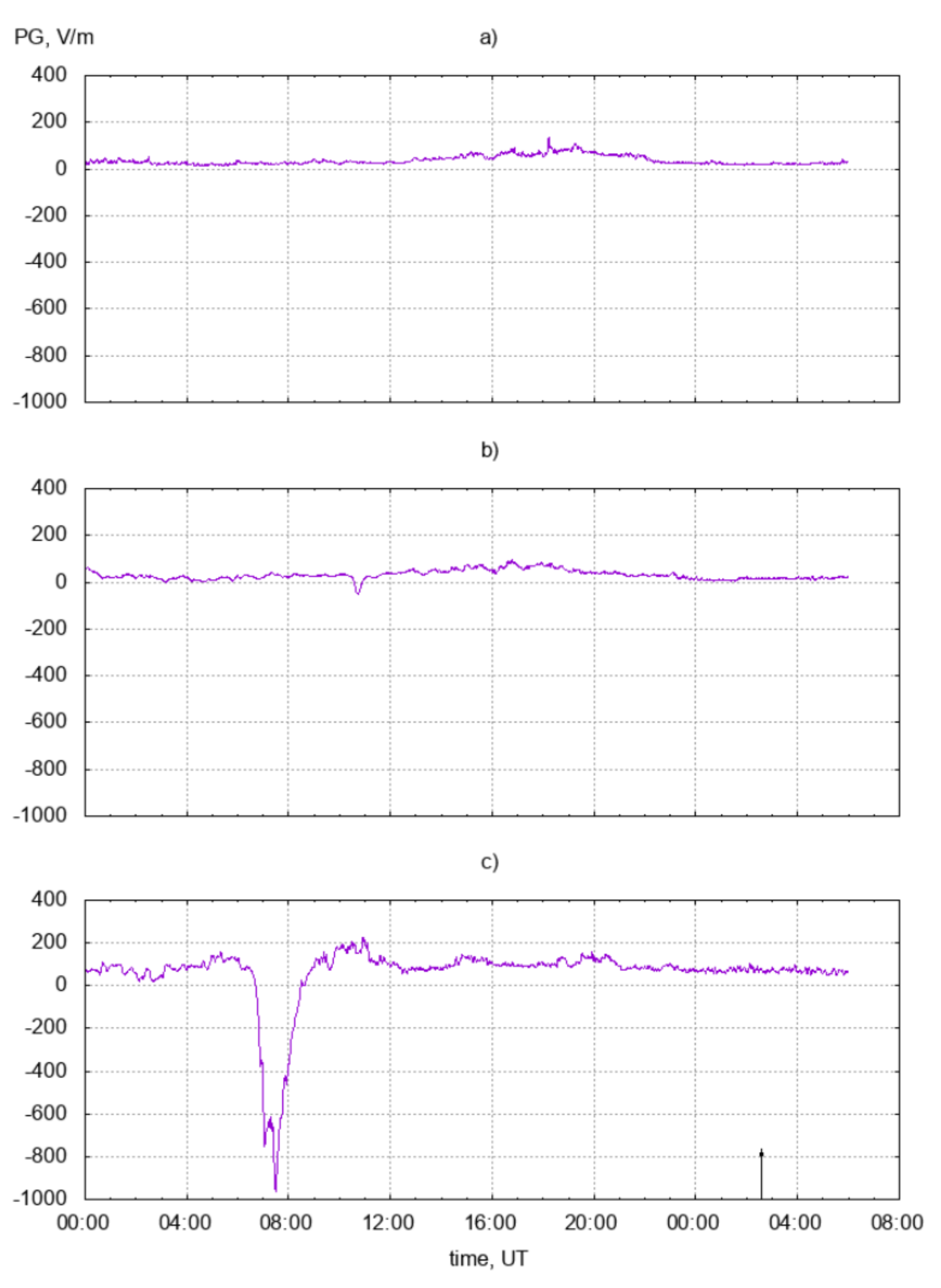
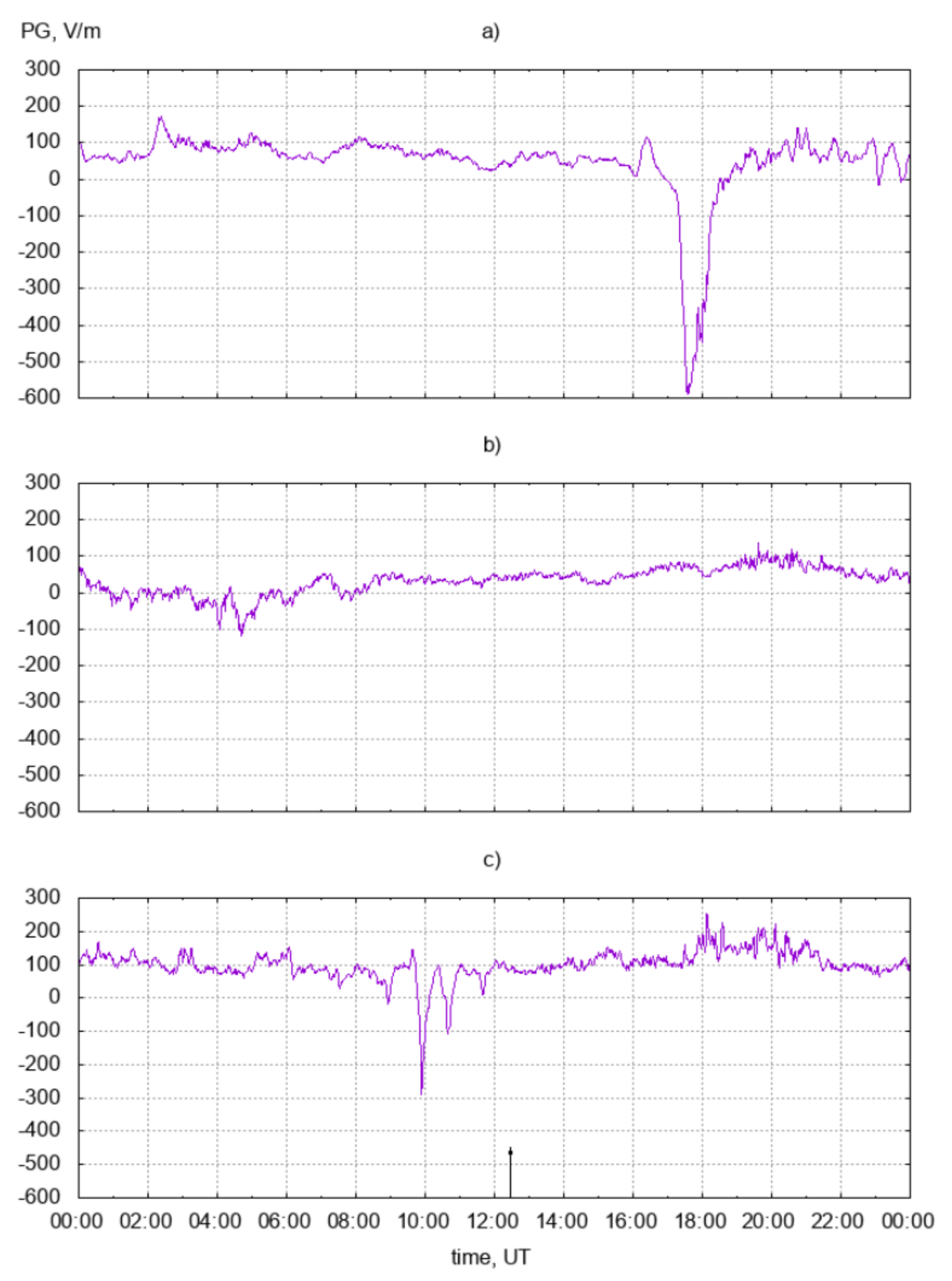
  • On small scales of time (T, hours) and distance, the bay duration and magnitude of the atmospheric potential gradient decrease was observed to depend on neither the earthquake class nor the distance to its epicenter;
  • On large scales of time (T, days) and distance (R), the precursor depended on the earthquake magnitude (M), according to the formula l g ( Δ T × R ) = a M + b
  • The efficiency of the forecast method for any weather condition was 10%.

Funding

This research was carried out according to the Russian State funding AAAA-A17-117080110043-4 “Dynamics of physical processes in the active zones of near space and geospheres”.

Acknowledgments

The authors are appreciative of “Paratunka” observatory FEBRAS.

Conflicts of Interest

The authors declare no conflict of interest. The funders had no role in the design of the study; in the collection, analyses, or interpretation of data; in the writing of the manuscript; nor in the decision to publish the results.

Abbreviations

The following abbreviations are used in this manuscript:
PGpotential gradient
EQearthquake

References

  1. Kondo, G. The variation of the atmospheric electric field at the time of earthquake. Kakioka Magnet. Observ. Mem. 1968, 13, 11–23. [Google Scholar]
  2. Kachakhidze, N.; Kachakhidze, M.; Kereselidze, Z.; Ramishvili, G. Specific variations of the atmospheric electric field potential gradient as a possible precursor of Caucasus earthquakes. Nat. Hazards Earth Syst. Sci. 2009, 9, 1221–1226. [Google Scholar] [CrossRef]
  3. Hao, J.G.; Tang, T.M.; Li, D.R. A kind of information on short-term and imminent earthquake precursors: - Research on atmospheric electric field anomalies before earthquakes. Acta Seismol. Sin. 1998, 11, 121–131. [Google Scholar] [CrossRef]
  4. Hao, J.; Tang, T.; Li, D. Progress in the research of atmospheric electric field anomaly as an index for short-impending prediction of earthquakes. J. Earthq. Pred. Res. 2000, 8, 241–255. [Google Scholar]
  5. Choudhury, A.; Guha, A.; De, B.K.; Roy, R. A statistical study on precursory effects of earthquakes observed through the atmospheric vertical electric field in northeast India. Ann. Geophys. 2013, 56, R0331. [Google Scholar]
  6. Harrison, R.G.; Aplin, K.L.; Rycroft, M.J. Atmospheric electricity coupling between earthquake regions and the ionosphere. J. Atmos. Sol. Terrest. Phys. 2010, 72, 376–381. [Google Scholar] [CrossRef] [Green Version]
  7. Liperovsky, V.A.; Pokhotelov, O.A.; Meister, C.V.; Liperovskaya, E.V. Physical models of coupling in the lithosphere–atmosphere–ionosphere system before earthquakes. Geomagnet. Aeron. 2008, 48, 795–806. [Google Scholar] [CrossRef]
  8. Pulinets, S.A.; Alekseev, V.A.; Legen’ka, A.D.; Khegai, V.V. Radon and metallic aerosols emanation before strong earthquakes and their role in atmosphere and ionosphere modification. Adv. Space Res. 1997, 20, 2173–2176. [Google Scholar] [CrossRef]
  9. Freund, F.T.; Kulahci, I.G.; Cyr, G.; Ling, J.; Winnick, M.; Tregloan-Reed, J.; Freund, M. Air ionization at rock surfaces and pre-earthquake signals. J. Atmos. Solar Terrest. Phys. 2009, 71, 1824–1834. [Google Scholar] [CrossRef]
  10. Pierce, E.T. Atmospheric electricity and earthquake prediction. J. Geophys. Lett. 1976, 3, 185–188. [Google Scholar] [CrossRef]
  11. Pulinets, S.A.; Boyarchuk, K.A. Ionospheric Precursors of Earthquakes; Springer: Berlin, Germany, 2004. [Google Scholar]
  12. Hoppel, W.A. Theory of electrode effect. J. Atmos. Terr. Phys. 1967, 29, 709–721. [Google Scholar] [CrossRef]
  13. Mikhailov, Y.M.; Mikhailova, G.A.; Kapustina, O.V.; Depueva, A.X.; Buzevich, A.V.; Druzhin, G.I.; Smirnov, S.E.; Firstov, P.P. Variations in different atmospheric and ionospheric parameters in the earthquake preparation periods on Kamchatka: Preliminary results. Geomagnet. Aeron. 2002, 42, 769–776. [Google Scholar]
  14. Pulinets, S.A.; Legen’ka, A.D.; Zelenova, T.I. Local time dependence of seismoionospheric variations in the F-layer Maimum. Geomagnet. Aeron. 1998, 38, 178–183. [Google Scholar]
  15. Pulinets, S.; Ouzounov, D. Lithosphere–atmosphere–ionosphere coupling (LAIC) model—An unified concept for earthquake precursors validation. J. Asian Earth Sci. 2011, 41, 371–382. [Google Scholar] [CrossRef]
  16. Pulinets, S. Low latitude atmosphere–ionosphere effects initiated by strong earthquakes preparation process. Int. J. Geophys. 2012, 2012, 131842. [Google Scholar] [CrossRef] [Green Version]
  17. Khomutov, S.; Smirnov, S.; Butin, S.; Babakhanov, I. First results of atmospheric electricity measurements by CS110 electric field meter at Paratunka observatory, Kamchatka. E3S Web Conf. 2016, 11, 00008. [Google Scholar] [CrossRef] [Green Version]
  18. Mikhailov, Y.M.; Mikhailova, G.A.; Kapustina, O.V.; Buzevich, A.V.; Smirnov, S.E. Specific features of atmospheric noise superimposed on variations in the quasistatic electric field in the Kamchatka near-earth atmosphere. Geomagnet. Aeron. 2005, 45, 649–664. [Google Scholar]
  19. Smirnov, S. Association of the negative anomalies of the quasistatic electric field in atmosphere with Kamchatka seismicity. Nat. Hazards Earth Syst. Sci. 2008, 8, 745–749. [Google Scholar] [CrossRef]
  20. Pustovalov, K.N.; Nagorskiy, P.M. Response in the surface atmospheric electric field to the passage of isolated air mass cumulonimbus clouds. J. Atmos. Solar Terrest. Phys. 2018, 172, 33–39. [Google Scholar] [CrossRef]
  21. Smirnov, S. Reaction of electric and meteorological states of the near-ground atmosphere during a geomagnetic storm on 5 April 2010. Earth Planet. Space 2014, 66, 154. [Google Scholar] [CrossRef] [Green Version]
  22. Sidorin, A.Y. Dependence of the Occurrence Time of Earthquake Precursors on the Epicentral Distance. Dokl. Akad. Nauk SSSR 1979, 245, 825–828. [Google Scholar]
  23. Korsunova, L.P.; Khegai, V.V.; Mikhailov, Y.M.; Smirnov, S.E. Regularities in the manifestation of earthquake precursors in the ionosphere and near-surface atmospheric electric fields in Kamchatka. Geomagnet. Aeron. 2013, 53, 227–233. [Google Scholar] [CrossRef]
Figure 1. Typical diurnal PG variations on days with fair weather conditions without anomalies (a), days with precipitation (b), and days with fair weather conditions, but with anomalous PG behavior (c). The arrow indicates the time of an earthquake that occurred on 24 September 1997, K = 11.4.
Geosciences 10 00010 g001
Figure 2. Negative anomalies of the potential gradient on 5 June 1999 (a), 8 July 1999 (b), and 24 October 1999 (c). The arrow indicates the time of an earthquake that occurred on 24 October 1999, K = 12.4.
Geosciences 10 00010 g002

