Interval Analysis of the Eigenvalues of Closed-Loop Control Systems with Uncertain Parameters

Abstract

Uncertainty caused by a parameter measurement error or a model error causes difficulties for the implementation of the control method. Experts can divide the uncertain system into a definite part and an uncertain part and solve each part using various methods. Two uncertainty problems of the control system arise: problem A for the definite part—how does one find out the optimal number and position of actuators when the actuating force of an actuator is smaller than the control force? Problem B for the uncertain part—how does one evaluate the effect of uncertainty on the eigenvalues of a closed-loop control system? This paper utilizes an interval to express the uncertain parameters and converts the control system into a definite part and an uncertain part using interval theory. The interval state matrix is constructed by physical parameters of the system for the definite part of the control system. For Problem A, the paper finds out the singular value element sensitivity of the modal control matrix and reorders the optimal location of the actuators. Then, the paper calculates the state feedback gain matrix for a single actuator using the receptance method of pole assignment and optimizes the number and position of the actuators using the recursive design method. For Problem B, which concerns the robustness of closed-loop systems, the paper obtains the effects of uncertain parameters on the real and imaginary parts of the eigenvalues of a closed-loop system using the matrix perturbation theory and interval expansion theory. Finally, a numerical example illustrates the recursive design method to optimize the number and location of actuators and it also shows that the change rate of eigenvalues increases with the increase in uncertainty.

1. Introduction

As a result of the complexity of structural, manufacturing and installation errors, and the inaccuracy of measurements, structural parameters are inevitably uncertain. This uncertainty may lead to a deterioration in vibration control performance. Therefore, the uncertainty of structural parameters plays an important role in vibration control [1]. However, uncertainty is not equal to stochasticity, and the stochastic method is not the only method for studying uncertain problems. In recent years, non-stochastic methods have been considered to analyze uncertain problems. The convex model theory is one such approach and has been applied by Dief to linear programming and system theory [2]. The convex model theory has attracted the attention of control theory and structural analysis workers. For example, Lindberg [3] discussed the dynamic response and failure problems of structures with the convex model, and Ganzerli [4] discussed the optimization problem of structure with uncertain parameters. Since the 1960s, the interval method [5] proposed by Moore has become an important tool for the analysis of uncertainty problems. Since the interval method requires little structural information and only needs to know the upper and lower bounds of structural parameters, it has attracted the attention of many scholars. The interval finite element method [6] is proposed by combining interval analysis with the finite element method, which makes it easier for interval analysis to deal with the analysis of complex structures. Great attention has also been paid to the problem of structural vibration control in engineering practice. Experts mainly discuss robustness when studying uncertain system control. Mori and Kokame [7] discussed the necessary and sufficient conditions for the dynamic stability of an uncertain system. Rachid [8] discussed the robust control of uncertain parameter systems.

The essence of vibration control is the assignment of poles and zero. The active control method has been applied to the assignment of poles and zero since the 1960s. Wonham [9] concluded that arbitrary poles can be assigned by state feedback when the structure is controllable. Datta [10] showed the explicit solution of the feedback gain matrix for calculating part of the eigenvalue assignment. In this algorithm, arbitrarily selected poles can be assigned for any controllable structure while the remaining poles remain unchanged. Duan [11] established two methods to obtain simple parametric equations of feedback gain and closed-loop eigenvalues with the aid of singular value decomposition and the factorization method. Ram and Mottershead [12] devised the receptance method of pole placement, where the vibration of the structure can be controlled and suppressed using the Sherman–Morrison formula and by means of measurement.

The configuration position of the actuator/sensor affects the performance of the closed-loop control system. Having fewer actuators and sensors is better for the sake of economic benefit. Therefore, it is of great value to determine the optimal number of actuators and sensors and to configure them at the optimal position. Many in-depth studies have been undertaken in this field [13,14,15,16,17,18,19,20,21,22,23,24] and can be divided into two aspects: one is to determine the optimal allocation criterion, or objective function to be optimized; the other is to select an appropriate optimization method. The optimal configuration criteria include the following: the maximum configuration criterion based on the singular value of the controllable matrix; the maximum configuration criterion of controllability/observability defined by the Grimm matrix; the configuration standards based on the minimum energy consumption of the system; the minimum configuration criterion based on control/observation overflow; the configuration criteria based on failure and reliability; the configuration standards based on the maximum response value in the time domain or the maximum response value in the frequency domain, etc. The optimal allocation algorithms are as follows: the non-linear planning optimization method, the sequential method, the simulated annealing method, the genetic algorithm, and the particle swarm optimization algorithm.

The objectives of the paper are as follows: (1) to establish the finite element equations for the uncertain system and divide them into a definite part and an uncertain part where uncertain parameters are treated as an interval using the interval theory in Section 2; (2) to find out the optimal position for each actuator according to the singular value element sensitivity of the modal control matrix in Section 3; (3) taking into consideration that the actual force is smaller than the ideal control force, to optimize the location and position for each actuator using the recursive method in Section 4; (4) to analyze the effect of uncertain parameters on the eigenvalues of the closed-loop system in Section 5; (4) to carry out an example to illustrate the proposed methods in Section 6.

2. Fundamental Equations for the Interval Analysis of Intelligent Structures

2.1. Finite Element Equations for Uncertain Systems

The following is the finite element equation of the intelligent structure with uncertain parameters [25,26,27,28,29,30]:

$$M\ddot{\Xi }(t)+C\dot{\Xi }(t)+K\Xi (t)=Du(t)+F(t),$$

(1)

where $M\in R^{n\times n}$ and $K\in R^{n\times n}$ are the mass and stiffness matrices of the intelligent structure, respectively; $C\in R^{n\times n}$ is the proportional damping matrix, $C=\alpha M+\beta K$, where α and β are the mass and stiffness proportional damping constants, respectively (more information can be found in [29]); $D\in R^{n\times n}$ is the control matrix determined by the position and number of actuators; $u(t)\in R^{n\times 1}$ is the control vector; $\Xi (t)\in R^{n\times 1}$ is the displacement vector; and $F(t)\in R^{n\times 1}$ is the mechanical force.

Divide the mass matrix, damping matrix, and stiffness matrix into definite parts and uncertain parts [25] to obtain:

$$M=M_0+\delta M,$$

(2)

$$C=C_0+\delta C,$$

(3)

$$K=K_0+\delta K,$$

(4)

where $M_0$, $C_0$, and $K_0$ are the definite parts of the mass matrix $M$, the damping matrix $C$, and stiffness matrix $K$, respectively; and $\delta M$, $\delta C$, and $\delta K$ are the uncertain parts of the aforementioned matrices, respectively.

Divide the displacement vector $\Xi \left(t\right)$, control vector $u\left(t\right)$, control matrix $D$, and mechanical force $F\left(t\right)$ into definite parts and uncertain parts in the same way [25], and we obtain:

$$\Xi \left(t\right)={\Xi }_0\left(t\right)+\delta \Xi \left(t\right),$$

(5)

$$u\left(t\right)=u_0\left(t\right)+\delta u\left(t\right),$$

(6)

$$D=D_0+\delta D,$$

(7)

$$F\left(t\right)=F_0\left(t\right)+\delta F\left(t\right),$$

(8)

where ${\Xi }_0\left(t\right)$, $u_0\left(t\right)$, $D_0$, and $F_0\left(t\right)$ are the definite parts of the displacement vector $\Xi \left(t\right)$, control vector $u\left(t\right)$, control matrix $D$, and mechanical force $F\left(t\right)$, respectively; $\delta C$, $\delta \Xi \left(t\right)$, $\delta u\left(t\right)$, $\delta D$, and $\delta F\left(t\right)$ are the uncertain parts of the above.

All through the paper, assume that the uncertainty is small, and that all uncertain parameters are expressed by the first-order Taylor approximation method according to the natural interval expansion principle and interval operation. Substituting Equations (2)–(8) into Equation (1), we have:

$$M_0{\ddot{\Xi }}_0\left(t\right)+C_0{\dot{\Xi }}_0\left(t\right)+K_0{\Xi }_0\left(t\right)=D_0{u}_0\left(t\right)+F_0\left(t\right),$$

(9)

$$\delta M{\ddot{\Xi }}_0\left(t\right)+M_0\delta \ddot{\Xi }\left(t\right)+\delta C{\dot{\Xi }}_0\left(t\right)+C_0\delta \dot{\Xi }\left(t\right)+\delta K{\Xi }_0\left(t\right)+K_0\delta \Xi \left(t\right)=\delta D{u}_0\left(t\right)+D_0\delta u\left(t\right)+\delta F\left(t\right).$$

(10)

The uncertain system equation (Equation (1)) is expressed by both the definite part equation (Equation (9)) and the uncertain part equation (Equation (10)).

2.2. Interval Mass Matrix, Interval Damping Matrix, and Interval Stiffness Matrix

Assume that the structural parameter $\mathsf{\gamma }$ has some degrees of error or uncertainty and is expressed as [5]:

$$\mathsf{\gamma }={\left[{\gamma }_1,{\gamma }_2,\cdots ,{\gamma }_{n1}\right]}^{\mathrm{T}},$$

(11)

where $n1$ is the number of uncertain parameters.

$\mathsf{\gamma }$ can be expressed by the following interval:

$$\mathsf{\gamma }={\mathsf{\gamma }}^c+\delta \mathsf{\gamma }\in {\mathsf{\gamma }}^I=\left[\underset{⌣}{\mathsf{\gamma }},\stackrel{⌢}{\mathsf{\gamma }}\right]=\left[{\mathsf{\gamma }}^c-\mathsf{\Delta }\mathsf{\gamma },{\mathsf{\gamma }}^c+\mathsf{\Delta }\mathsf{\gamma }\right]=\left[{\mathsf{\gamma }}^c,{\mathsf{\gamma }}^c\right]+\left[-\mathsf{\Delta }\mathsf{\gamma },\mathsf{\Delta }\mathsf{\gamma }\right]={\mathsf{\gamma }}^c+\mathsf{\Delta }{\mathsf{\gamma }}^I,$$

(12)

where $\delta \mathsf{\gamma }$ is the uncertain part of $\mathsf{\gamma }$; ${\mathsf{\gamma }}^I=\left[\underset{⌣}{\mathsf{\gamma }},\stackrel{⌢}{\mathsf{\gamma }}\right]$ is the interval parameter; $\underset{⌣}{\mathsf{\gamma }}={\mathsf{\gamma }}^c-\mathsf{\Delta }\mathsf{\gamma }$ is the left end point of interval ${\mathsf{\gamma }}^I$; $\stackrel{⌢}{\mathsf{\gamma }}={\mathsf{\gamma }}^c+\mathsf{\Delta }\mathsf{\gamma }$ is the right end point of interval ${\mathsf{\gamma }}^I$; ${\mathsf{\gamma }}^c=\left(\underset{⌣}{\mathsf{\gamma }}+\stackrel{⌢}{\mathsf{\gamma }}\right)/2$ is the midpoint of interval ${\mathsf{\gamma }}^I$; $\mathsf{\Delta }\mathsf{\gamma }=\left(\stackrel{⌢}{\mathsf{\gamma }}-\underset{⌣}{\mathsf{\gamma }}\right)/2$ is the radius of interval ${\mathsf{\gamma }}^I$.

For any $\mathsf{\gamma }\in {\mathsf{\gamma }}^I$, when the interval parameter $\mathsf{\gamma }$ has a small disturbance around the median value ${\mathsf{\gamma }}^c$, the first-order approximations of $M\left(\mathsf{\gamma }\right)$, $C\left(\mathsf{\gamma }\right)$, and $K\left(\mathsf{\gamma }\right)$ are obtained by expansion using the Taylor approximation near ${\mathsf{\gamma }}^c$ [25].

We also have [5]:

$$M\left({\mathsf{\gamma }}^I\right)=M\left({\mathsf{\gamma }}^c\right)+\mathsf{\Delta }M\left({\mathsf{\gamma }}^I\right),$$

(13)

$$C\left({\mathsf{\gamma }}^I\right)=C\left({\mathsf{\gamma }}^c\right)+\mathsf{\Delta }C\left({\mathsf{\gamma }}^I\right),$$

(14)

$$K\left({\mathsf{\gamma }}^I\right)=K\left({\mathsf{\gamma }}^c\right)+\mathsf{\Delta }K\left({\mathsf{\gamma }}^I\right),$$

(15)

where $M\left({\mathsf{\gamma }}^I\right)$, $C\left({\mathsf{\gamma }}^I\right)$, and $K\left({\mathsf{\gamma }}^I\right)$ are the interval mass matrix, the interval damping matrix, and the interval stiffness matrix, respectively; $M\left({\mathsf{\gamma }}^c\right)$, $C\left({\mathsf{\gamma }}^c\right)$, and $K\left({\mathsf{\gamma }}^c\right)$ are the median mass matrix, the median damping matrix, and the median stiffness matrix of the structure, respectively. $\mathsf{\Delta }M\left({\mathsf{\gamma }}^I\right)$, $\mathsf{\Delta }C\left({\mathsf{\gamma }}^I\right)$, and $\mathsf{\Delta }K\left({\mathsf{\gamma }}^I\right)$ are the first-order increment matrix of the interval mass matrix, interval damping matrix, and interval stiffness matrix, respectively:

$$\mathsf{\Delta }M\left({\mathsf{\gamma }}^I\right)={\displaystyle \sum _{l=1}^{n1}\frac{\partial M\left({\mathsf{\gamma }}^c\right)}{\partial {\gamma }_l^I}\left({\gamma }_l^I-{\gamma }_l^c\right)},$$

(16)

$$\mathsf{\Delta }C\left({\mathsf{\gamma }}^I\right)={\displaystyle \sum _{l=1}^{n1}\frac{\partial C\left({\mathsf{\gamma }}^c\right)}{\partial {\gamma }_l^I}\left({\gamma }_l^I-{\gamma }_l^c\right)},$$

(17)

$$\mathsf{\Delta }K\left({\mathsf{\gamma }}^I\right)={\displaystyle \sum _{l=1}^{n1}\frac{\partial K\left({\mathsf{\gamma }}^c\right)}{\partial {\gamma }_l^I}\left({\gamma }_l^I-{\gamma }_l^c\right)},$$

(18)

Equation (10) can also be expressed as:

$$\begin{array}{l}\mathsf{\Delta }{M}^I{\ddot{\Xi }}_0\left(t\right)+M_0\mathsf{\Delta }{\ddot{\Xi }}^I\left(t\right)+\mathsf{\Delta }{C}^I{\dot{\Xi }}_0\left(t\right)+C_0\mathsf{\Delta }{\dot{\Xi }}^I\left(t\right)+\mathsf{\Delta }{K}^I{\Xi }_0\left(t\right)+K_0\mathsf{\Delta }{\Xi }^I\left(t\right)=\\ \mathsf{\Delta }{D}^I{u}_0\left(t\right)+D_0\mathsf{\Delta }{u}^I\left(t\right)+\mathsf{\Delta }{F}^I\left(t\right)\end{array},$$

(19)

2.3. State Equation of the Uncertain System with/without Feedback Control

The state equation for the uncertain structure equation (Equation (1)) is:

$$\dot{X}\left(t\right)=AX\left(t\right)+Bu\left(t\right)+\eta \left(t\right),$$

(20)

where $X\left(t\right)={\left[{\Xi }^{\mathrm{T}}\left(t\right),\hspace{1em}{\dot{\Xi }}^{\mathrm{T}}\left(t\right)\right]}^{\mathrm{T}}$ is the state vector; $u\left(t\right)=G^{\mathrm{T}}X\left(t\right)$ is the input vector of the state feedback control; and $G\in R^{p\times 2n}$ is the state feedback gain matrix. The state matrix $A\in R^{2n\times 2n}$, and the distribution matrix of the actuators $B\in R^{2n\times p}$ and $\eta \left(t\right)$ are:

$$A=\left[\begin{array}{cc}0& I\\ -M^{-1}K& -M^{-1}C\end{array}\right], B=\left[\begin{array}{l}0\\ D\end{array}\right], \eta \left(t\right)=\left[\begin{array}{l}0\\ F\left(t\right)\end{array}\right].$$

The state equation (Equation (20)) of the uncertain structure in the closed-loop system can also written as:

$$\dot{X}\left(t\right)=\left(A+B{G}^{\mathrm{T}}\right)X\left(t\right)+\eta \left(t\right).$$

(21)

The corresponding eigenvalue problem for Equation (21) is:

$$\left(A+B{G}^{\mathrm{T}}\right){\widehat{W}}_j={\widehat{S}}_j{\widehat{W}}_j,$$

(22)

$${\left(A+B{G}^{\mathrm{T}}\right)}^{\mathrm{H}}{\widehat{V}}_j={\overline{\widehat{S}}}_j{\widehat{V}}_j,$$

(23)

where ${\widehat{S}}_j$ is the $j$-th order complex eigenvalue of the closed-loop system with an uncertain structure; ${\widehat{W}}_j$ and ${\widehat{V}}_j$ are the corresponding right and left eigenvectors; the superscript $\mathrm{H}$ is the conjugate transpose; and ${\overline{\widehat{S}}}_j$ is the conjugate of ${\widehat{S}}_j$.

The control system of the uncertain structure is as follows:

$$A=A_0+\delta A,$$

(24)

$$B=B_0+\delta B,$$

(25)

where $A_0$ and $B_0$ are the definite parts of $A$ and $B$, respectively; and $\delta A$ and $\delta B$ are the uncertain parts:

$$\begin{array}{c}{A}_0=\left[\begin{array}{cc}0& I\\ -M_0^{-1}{K}_0& -M_0^{-1}{C}_0\end{array}\right],\delta A=\left[\begin{array}{cc}0& I\\ -\left(M_0^{-1}\delta K+\delta M^{-1}{K}_0\right)& -\left(M_0^{-1}\delta C+\delta M^{-1}{C}_0\right)\end{array}\right],\\ B_0=\left[\begin{array}{c} 0\\ D_0\end{array}\right],\delta B=\left[\begin{array}{c} 0\\ \delta D\end{array}\right].\end{array}$$

The state vector $X\left(t\right)$ and feedback gain matrix $G$ are as follows:

$$X\left(t\right)=X_0\left(t\right)+\delta X\left(t\right),$$

(26)

$$G=G_0+\delta G,$$

(27)

where $X_0\left(t\right)$ and $G_0$ are the definite parts of the state vector and the feedback gain matrix, respectively; and $\delta X\left(t\right)$ and $\delta G$ are the uncertain parts.

By substituting Equations (24)–(27) into Equation (21) and ignoring the terms of the higher order, we obtain:

$${\dot{X}}_0\left(t\right)=A_0{X}_0\left(t\right)+B_0{u}_0\left(t\right)+{\eta }_0\left(t\right),$$

(28)

$$u_0\left(t\right)=G_0^{\mathrm{T}}{X}_0\left(t\right),$$

(29)

$$\delta \dot{X}\left(t\right)=A_0\delta X\left(t\right)+\delta A{X}_0\left(t\right)+B_0\delta u\left(t\right)+\delta B{u}_0\left(t\right),$$

(30)

$$\delta u\left(t\right)=G_0^{\mathrm{T}}\delta X\left(t\right)+\delta G^{\mathrm{T}}{X}_0\left(t\right).$$

(31)

We divided the control system into the definite parts, as in Equations (28) and (29), and the uncertain parts, as in Equations (30) and (31).

From Equations (28) and (29), the state equation of the definite part of the closed-loop system can be written as:

$${\dot{X}}_0\left(t\right)=\left(A_0+B_0{G}_0^{\mathrm{T}}\right)X_0\left(t\right)+{\eta }_0\left(t\right).$$

(32)

The corresponding eigenvalue problem for the definite part of the closed-loop system is:

$$\left(A_0+B_0{G}_0^{\mathrm{T}}\right){\widehat{W}}_{0j}={\widehat{S}}_{0j}{\widehat{W}}_{0j},$$

(33)

$${\left(A_0+B_0{G}_0^{\mathrm{T}}\right)}^{\mathrm{H}}{\widehat{V}}_{0j}={\overline{\widehat{S}}}_{0j}{\widehat{V}}_{0j},$$

(34)

where ${\widehat{S}}_{0j}$ is the complex eigenvalues of the $j\text{-}\mathrm{th}$ order for definite closed-loop systems; ${\widehat{W}}_{0j}$ and ${\widehat{V}}_{0j}$ are the corresponding right and left eigenvectors; the superscript $\mathrm{H}$ is the conjugate transpose; and ${\overline{\widehat{S}}}_{0j}$ is the conjugate of ${\widehat{S}}_{0j}$.

Systems with uncertain parameters can be considered as perturbations of systems with certain parameters. The interval response $X^I\left(t\right)$ is:

$$X^I\left(t\right)=X_0\left(t\right)+\mathsf{\Delta }{X}^I\left(t\right),$$

(35)

where $X_0\left(t\right)$ is determined by Equation (32).

The interval state matrix and interval control matrix are [25]:

$$A^I=A_0+\mathsf{\Delta }{A}^I,$$

(36)

$$B^I=B_0+\mathsf{\Delta }{B}^I,$$

(37)

where $A^I=A\left({\mathsf{\gamma }}^I\right)$ and $B^I=B\left({\mathsf{\gamma }}^I\right)$ are the interval state matrix and interval control matrix; $\mathsf{\Delta }{A}^I=\mathsf{\Delta }A\left({\mathsf{\gamma }}^I\right)$ is the first-order increment matrix of the interval state matrix; and $\mathsf{\Delta }{B}^I=\mathsf{\Delta }B\left({\mathsf{\gamma }}^I\right)$ is the first-order increment matrix of the interval control matrix:

$$\mathsf{\Delta }{A}^I=\left[\begin{array}{cc}0& I\\ -M_0^{-1}\mathsf{\Delta }{K}^I-{\left(\mathsf{\Delta }{M}^I\right)}^{-1}{K}_0& -M_0^{-1}\mathsf{\Delta }{C}^I-{\left(\mathsf{\Delta }{M}^I\right)}^{-1}{C}_0\end{array}\right],\mathsf{\Delta }{B}^I=\left[\begin{array}{c}0\\ \mathsf{\Delta }{D}^I\end{array}\right].$$

The interval gain matrix $G^I$ is:

$$G^I=G_0+\mathsf{\Delta }{G}^I.$$

(38)

$\mathsf{\Delta }{X}^I\left(t\right)$ in Equation (35) is determined by the following equation:

$$\mathsf{\Delta }{\dot{X}}^I\left(t\right)=A_0\mathsf{\Delta }{X}^I\left(t\right)+\mathsf{\Delta }{A}^I{X}_0\left(t\right)+B_0\mathsf{\Delta }{u}^I\left(t\right)+\mathsf{\Delta }{B}^I{u}_0\left(t\right).$$

(39)

In order to study the response of the system with uncertain parameters, we treat the control problem of the definite parameter system using Equation (32), and then study the influence of the uncertain parameters on the control using Equation (39).

In Section 3, the paper proposes a method to judge which position is the optimal position for a single input. In Section 4, a recursive design method is introduced to optimize the location and number of actuators when the actual control force is smaller than the ideal control force. In Section 5, the paper discusses the effect of uncertainty on eigenvalues of the closed-loop system using interval analysis.

3. Optimization of Actuator Position in Vibration Control of Intelligent Structure

3.1. The Measure of the Modal Controllability of Intelligent Structures

Equation (9) is the vibration control equation of the system with certain parameters. Although the original equation has n modes, the vibration of sub-systems with lower eigenvalues is much larger than that with higher eigenvalues, and we only need to control the vibration of the sub-systems with lower r eigenvalues and ignore the vibration of those with higher eigenvalues. Generally the (r + 1)-th eigenvalue is much larger than exciting frequency. Transfer Equation (9) into the modal coordinate system for the purpose of modal control and, according to the modal expansion theorem, we have:

$${\Xi }_0\left(t\right)=p_0{q}_0\left(t\right),$$

(40)

where $q_0\left(t\right)\in R^{r\times 1}$ is the modal coordinate vector; $p_0\in R^{n\times r}$ is the modal matrix; and $r$ is the number of modes intercepted.

Substitute Equation (40) into Equation (9) and multiply both sides of the equation by $p_0^{\mathrm{T}}$ to the left, and we have:

$$M_0^{*}{\ddot{q}}_0\left(t\right)+C_0^{*}{\dot{q}}_0\left(t\right)+K_0^{*}{q}_0\left(t\right)=D_0^{*}u\left(t\right)+F_0^{*}\left(t\right),$$

(41)

where $M_0^{*}=p_0^{\mathrm{T}}{M}_0{p}_0$ is the modal mass matrix, $M_0^{*}\in R^{r\times r}$; $C_0^{*}=p_0^{\mathrm{T}}{C}_0{p}_0$ is the modal damping matrix, $C_0^{*}\in R^{r\times r}$; $K_0^{*}=p_0^{\mathrm{T}}{K}_0{p}_0$ is the modal stiffness matrix, $K_0^{*}\in R^{r\times r}$; $D_0^{*}=p_0^{\mathrm{T}}{D}_0\in R^{r\times n}$ is the modal control matrix; and $F_0^{*}\left(t\right)=p_0^{\mathrm{T}}{F}_0\left(t\right)$ is the mechanical forces in the modal coordinates.

A problem is that Equation (41) cannot reflect the direct relationship between control force $u_0\left(t\right)$ and mode controllability. To solve this problem, decompose modal control matrix $D_0^{*}\in R^{r\times n}$ using the Singular Value Decomposition (SVD) method:

$$D_0^{*}={\Phi }_0{\Sigma }_0{\Psi }_0^{\mathrm{T}},$$

(42)

where the columns of the orthogonal matrix ${\Phi }_0\in R^{r\times r}$ (${\Phi }_0^{\mathrm{T}}{\Phi }_0=I_r$) are the left singular vector of $D_0^{*}$; the columns of the orthogonal matrix ${\Psi }_0\in R^{n\times n}$ (${\Psi }_0^{\mathrm{T}}{\Psi }_0=I_n$) are the right singular vector of $D_0^{*}$; ${\Sigma }_{0r}=diag\left({\sigma }_{01},{\sigma }_{02},\cdots ,{\sigma }_{0r}\right)$ is the diagonal matrix of non-zero elements in ${\Sigma }_0$; ${\sigma }_{01}\ge {\sigma }_{02}\ge \cdots \ge {\sigma }_{0r}>0$; ${\sigma }_{0j}$ $\left(j=1,2,\cdots ,r\right)$ is the singular value of $D_0^{*}$; and $I_r$ is the identity matrix of the order $r$.

Multiply both sides of Equation (42) by ${\Phi }_0^{\mathrm{T}}$ and consider $D_0^{*}=p_0^{\mathrm{T}}{D}_0$, and we obtain:

$${\Phi }_0^{\mathrm{T}}{p}_0^{\mathrm{T}}{B}_0={\Sigma }_0{V}_0^{\mathrm{T}}.$$

(43)

A new set of coordinates ${\tilde{q}}_0\left(t\right)$ is introduced to measure the controllability of modes by ${\Sigma }_0$:

$${\Xi }_0\left(t\right)=p_0{\Phi }_0{\tilde{q}}_0\left(t\right).$$

(44)

Substitute Equation (44) into Equation (41), and we obtain:

$${\tilde{M}}_0^{*}{\ddot{\tilde{q}}}_0\left(t\right)+{\tilde{C}}_0^{*}{\dot{\tilde{q}}}_0\left(t\right)+{\tilde{K}}_0^{*}{\tilde{q}}_0\left(t\right)={\Sigma }_0{\tilde{u}}_0\left(t\right)+{\tilde{F}}_0^{*}\left(t\right),$$

(45)

where ${\tilde{M}}_0^{*}={\Phi }_0^{\mathrm{T}}{p}_0^{\mathrm{T}}{M}_0{p}_0{\Phi }_0$ (${\tilde{M}}_0^{*}\in R^{r\times r}$), ${\tilde{C}}_0^{*}={\Phi }_0^{\mathrm{T}}{p}_0^{\mathrm{T}}{C}_0{p}_0{\Phi }_0$ (${\tilde{C}}_0^{*}\in R^{r\times r}$), ${\tilde{K}}_0^{*}={\Phi }_0^{\mathrm{T}}{p}_0^{\mathrm{T}}{K}_0{p}_0{\Phi }_0$ (${\tilde{K}}_0^{*}\in R^{r\times r}$), and ${\tilde{F}}_0^{*}\left(t\right)$=${\Phi }_0^{\mathrm{T}}{p}_0^{\mathrm{T}}{F}_0\left(t\right)$ (${\tilde{F}}_0^{*}\left(t\right)\in R^{r\times 1}$) are the mass matrix, damping matrix, stiffness matrix, and mechanical force in the $p_0{\Phi }_0$ space, respectively; ${\tilde{u}}_0\left(t\right)={\Psi }_0^{\mathrm{T}}{u}_0\left(t\right)$. As ${\Psi }_0^{\mathrm{T}}{\Psi }_0=I_n$, $u_0\left(t\right)$ and ${\tilde{u}}_0\left(t\right)$ are equivalent in a modular sense. The controllability of ${\tilde{q}}_0\left(t\right)$ can be measured by ${\sigma }_{0j}$ in ${\Sigma }_0$: the larger ${\sigma }_{0j}$ is, the stronger the control effect on ${\tilde{q}}_0\left(t\right)$ and the less energy is consumed.

3.2. Singular Value Element Sensitivity of Modal Control Matrix $D_0^{*}$

When the number of controlled modes is $r$ and the number of actuators is $n$, from Equation (42), we have [17,31]:

$$D_0^{*}{D}_0^{*\mathrm{T}}{\Phi }_0={\Phi }_0{\Sigma }_0{\Sigma }_0^{\mathrm{T}}.$$

(46)

Remove the actuator on the $i\text{-}\mathrm{th}$ unit from the current structure, and Equation (46) becomes:

$${\tilde{D}}_0^{*i}{\tilde{D}}_0^{*i\mathrm{T}}{\tilde{\Phi }}_0^i={\tilde{\Phi }}_0^i{\tilde{\Sigma }}_0^i{\tilde{\Sigma }}_0^{i\mathrm{T}},$$

(47)

or

$${\tilde{D}}_0^{*i}{\tilde{D}}_0^{*i\mathrm{T}}{\tilde{\Phi }}_{0j}^i={\tilde{\Phi }}_{0j}^i{\left({\tilde{\sigma }}_{0j}^i\right)}^2.$$

(48)

It is necessary to perform a perturbation calculation for Equation (46) in order to obtain the optimal position of the actuator using the topology optimization method. According to perturbation theory, the eigenvalues and eigenvectors represented by Equation (48) can be expressed as the power series of the small parameter $\epsilon$:

$${\tilde{D}}_0^{*i}=D_0^{*}+\epsilon D_{01}^{*i},$$

(49)

$${\tilde{\sigma }}_{0j}^i={\sigma }_{0j}+\epsilon {\sigma }_{01j}^i+{\epsilon }^2{\sigma }_{02j}^i+\cdots ,$$

(50)

$${\tilde{\Phi }}_{0j}^i={\Phi }_{0j}+\epsilon {\Phi }_{01j}^i+{\epsilon }^2{\Phi }_{02j}^i+\cdots ,$$

(51)

where ${\tilde{D}}_0^{*i}$ is the modal control matrix when moving the actuator on the $i\text{-}\mathrm{th}$ element; the $j\text{-}\mathrm{th}$ column ${\tilde{\Phi }}_{0j}^i$ of orthogonal matrix ${\tilde{\Phi }}_0^i$ is the left singular vector of the $j\text{-}\mathrm{th}$ order; when removing the actuator on the $i\text{-}\mathrm{th}$ element, ${\sigma }_{0j}$ and ${\Phi }_{0j}$ are the $j\text{-}\mathrm{th}$ order singular value and $j\text{-}\mathrm{th}$ order left singular vector of the original system, respectively; ${\sigma }_{01j}^i$ and ${\sigma }_{02j}^i$ are respectively the first-order and second-order perturbations of singular value ${\sigma }_{0j}$ when removing the actuator on the $i\text{-}\mathrm{th}$ element; and ${\Phi }_{01j}^i$ and ${\Phi }_{02j}^i$ are, respectively, the first-order and second-order perturbations of the $j\text{-}\mathrm{th}$ order left singular vector ${\Phi }_{0j}$ when removing actuator on the $i\text{-}\mathrm{th}$ element.

To solve Equation (48), the first-order perturbation momentum of eigenvalues is:

$${\sigma }_{01j}^i=\sqrt{{\Phi }_{0j}^{\mathrm{T}}\left(B_0{B}_{01}^{i\mathrm{T}}+B_{01}^{i\mathrm{T}}{B}_0\right){\Phi }_{0j}},$$

(52)

where ${\sigma }_{01j}^i$ is the element sensitivity contribution to the singular value of the $j\text{-}\mathrm{th}$ modal control matrix when the actuator on $i\text{-}\mathrm{th}$ element is removed.

3.3. Control Position Optimization Criteria

For intelligent structures, when the $i\text{-}\mathrm{th}$ actuators are removed, the singular value and singular vector of each order will change. When the actuator on the $i\text{-}\mathrm{th}$ unit is removed, we define ${\Omega }_{ai}$ as follows [17]:

$${\Omega }_{ai}={\displaystyle \sum _{j=1}^r{\sigma }_{01j}^i}, {\Omega }_a=\left[{\Omega }_{a1},{\Omega }_{a2},\cdots ,{\Omega }_{an}\right],$$

(53)

which is a measure of actuator position optimization. ${\Omega }_{ai}$ is the sum of the singular value sensitivity contributions to the modal control matrix. The dimensionless optimization metric ${\tilde{\Omega }}_{ai}$ of the $i\text{-}\mathrm{th}$ actuator position and sorted in the form of matrix ${\tilde{\Omega }}_a$ is as follows:

$${\tilde{\Omega }}_{ai}={\Omega }_{ai}/\max ({\Omega }_{a1},{\Omega }_{a2},\cdots ,{\Omega }_{an}), \left(i=1,2,\cdots ,n\right),$$

(54)

$${\tilde{\Omega }}_a=\left[{\tilde{\Omega }}_{a1},{\tilde{\Omega }}_{a2},\cdots ,{\tilde{\Omega }}_{an}\right],$$

(55)

where $\max ({\Omega }_{a1},{\Omega }_{a2},\cdots ,{\Omega }_{an})$ is the largest absolute value of element in ${\Omega }_a$; and ${\tilde{\Omega }}_a$ is also dimensionless. The criteria for intelligent structure actuator location optimization is:

$${\tilde{\Omega }}_a\ge \tilde{\Omega },$$

(56)

where $\tilde{\Omega }$ is a given threshold. If the optimization criteria in Equation (56) is met, the actuator on the $i\text{-}\mathrm{th}$ element is preserved. Otherwise, the actuator on the $i\text{-}\mathrm{th}$ element is removed from the structure. Let $i=i+1$ and repeat the above steps to determine the optimal number and location of actuators. Obviously, the bigger $\tilde{\Omega }$ is, the fewer actuators are placed.

4. The Recursive Design Method of Multi-Input Modal Controller

4.1. Required Control Force Calculation Based on the Receptance Method

The state equation for the definite closed-loop system is Equation (32). In this section, the receptance method will be used to calculate the control force and feedback gain matrix for a single input [32].

Considering the condition of a single input, $B_0$ is the column vector and $G_0^{\mathrm{T}}$ is the row vector. With modal transformation $X_0\left(t\right)=W_0{\xi }_0\left(t\right)$, we have the following modal governing equation:

$${\dot{\xi }}_0\left(t\right)=\left({\Lambda }_0+B_0^{*}{G}_0^{*\mathrm{T}}\right){\xi }_0\left(t\right)+{\eta }_0^{*}\left(t\right),$$

(57)

where ${\xi }_0\left(t\right)$ is modal coordinate vector, ${\xi }_0\left(t\right)\in R^{2r\times 1}$; ${\Lambda }_0=V_0^{\mathrm{H}}{A}_0{W}_0$ is eigenvalue matrix of the state matrix ${\Lambda }_0\in R^{2r\times 2r}$; $W_0$ and $V_0$ are the right and left mode matrices of the state matrix $A_0$, respectively; and $V_0^{\mathrm{H}}{U}_0=I_r$; $B_0^{*}=V_0^{\mathrm{H}}{B}_0$ is modal control matrix in state space; and $G_0^{*\mathrm{T}}$=$G_0^{\mathrm{T}}{W}_0$ is modal gain matrix in state space.

Equation (57) can be written as:

$${\dot{\xi }}_0\left(t\right)-\left({\Lambda }_0+B_0^{*}{G}_0^{*\mathrm{T}}\right){\xi }_0\left(t\right)={\eta }_0^{*}\left(t\right).$$

(58)

Transfer Equation (58) into the Laplace domain, and we have:

$$\left(S-{\Lambda }_0-B_0^{*}{G}_0^{*\mathrm{T}}\right){\xi }_0\left(S\right)={\eta }_0^{*}\left(S\right).$$

(59)

The Sherman–Morrison formula [12] is as follows:

$$\widehat{H}\left(S\right)=H\left(S\right)-\frac{H\left(S\right)B_0^{*}{G}_0^{*\mathrm{T}}H\left(S\right)}{1+G_0^{*\mathrm{T}}H\left(S\right)B_0^{*}},$$

(60)

where $\widehat{H}\left(S\right)={\left(S-{\Lambda }_0-B_0^{*}{G}_0^{*\mathrm{T}}\right)}^{-1}$ is the receptance matrix of the closed-loop system. $H\left(S\right)={\left(S-{\Lambda }_0\right)}^{-1}$ is the receptance matrix of the open-loop system. The characteristic polynomials of closed-loop systems are $1+G_0^{*\mathrm{T}}H\left(S\right)B_0^{*}$. If we want to assign the poles to ${\Lambda }_0^{*}=\left[{\lambda }_{01}^{*},{\lambda }_{02}^{*},\cdots ,{\lambda }_{02r}^{*}\right]$, let the denominator of Equation (60) be zero:

$$1+G_0^{*\mathrm{T}}H\left({\Lambda }_0^{*}\right)B_0^{*}=0.$$

(61)

The feedback gain matrix $G_0^{*}$ can be obtained by solving Equation (61). Multiply $X_0\left(t\right)=W_0{\xi }_0\left(t\right)$ by $V_0^{\mathrm{H}}$, and we have:

$${\xi }_0\left(t\right)=V_0^{\mathrm{H}}{X}_0\left(t\right).$$

(62)

Substitute Equation (62) into Equation (29), and we have:

$$u_0\left(t\right)=G_0^{*\mathrm{T}}{V}_0^{\mathrm{H}}{X}_0\left(t\right)=G_0^{\mathrm{T}}{X}_0\left(t\right),$$

(63)

and

$$G_0^{\mathrm{T}}=G_0^{*\mathrm{T}}{V}_0^{\mathrm{H}}.$$

(64)

When the structure is fully controllable for the single-input system, from Equations (63) and (64), we can calculate the required control force $u_0\left(t\right)$ and the state feedback gain matrix $G_0$.

4.2. Optimal Number and Location of Actuators When the Actual Control Force Is Smaller than the Required Control Force

Generally, the actuators are the same and the range of execution force for each one is:

$${\tilde{u}}_{01}\left(t\right)\in \left[-a1 a1\right],$$

(65)

where $a1$ is the maximum execution force. We will discuss the optimal number and location of the actuators, with special consider for the condition that the actual control force is smaller than the required force.

• If $\left|u_{01}\left(t\right)\right|<a1$, one actuator can provide the feedback gain required by the controlled structure in excess;
• If $\left|u_{01}\left(t\right)\right|=a1$, one actuator just provides the feedback gain required by the controlled structure;
• If $\left|u_{01}\left(t\right)\right|>a1$, the single-input control cannot make the structure fully controllable and multiple actuators are needed to provide sufficient feedback gain to make the structure fully controllable.

For the case of $\left|u_{01}\left(t\right)\right|\le a1$, only a single input can satisfy the requirement. However, for the case of $\left|u_{01}\left(t\right)\right|>a1$, a multi-input control should be introduced to make the structure fully controllable [33].

We will determine the minimum number and optimal location of actuators required using the recursive design method for a multi-input modal controller. Assume $b_1$, $b_2$, …, $b_{\Theta }$ are the optional, sub-optional, and the $\tau \text{-}\mathrm{th}$ optional positions for $\tau$ actuators. Construct the state equation of the structure as:

$${\dot{X}}_0\left(t\right)=A_0{X}_0\left(t\right)+{\displaystyle \sum _{\tau =1}^{\Theta }{B}_{0\tau }{\tilde{u}}_{0\tau }\left(t\right)}+{\eta }_0\left(t\right).$$

(66)

Adopt the state feedback control, and we have:

$${\tilde{u}}_{0\tau }\left(t\right)={\tilde{G}}_{0\tau }^T{X}_0\left(t\right).$$

(67)

Substitute Equation (67) into Equation (66), and we have:

$${\dot{X}}_0\left(t\right)=\left(A_0+{\displaystyle \sum _{\tau =1}^{\Theta }{B}_{0\tau }{\tilde{G}}_{0\tau }^T}\right)X_0\left(t\right)+{\eta }_0\left(t\right),$$

(68)

where ${\tilde{u}}_{0\tau }\left(t\right)$ is the actual input vector in the $\tau \text{-}\mathrm{th}$ step; $B_{0\tau }$ is distribution matrix of the actuator in the $\tau \text{-}\mathrm{th}$ step; ${\tilde{G}}_{0\tau }$ is the actual gain provided by the actuator in the $\tau \text{-}\mathrm{th}$ step. Then, we can solve the following state equation:

$${\dot{X}}_0\left(t\right)=\left(A_0+{\displaystyle \sum _{\tau =1}^{\Theta }{B}_{0\tau }{\tilde{G}}_{0\tau }^T}\right)X_0\left(t\right).$$

(69)

The complex eigenvalue is ${\tilde{\Lambda }}_{0\tau }$, compare it to the eigenvalue that is to be configured. When ${\tilde{\Lambda }}_{0\tau }={\Lambda }_0^{*}$, stop the recursive design and $\tau$ is the minimum number of actuators.

5. Interval Analysis of the Robustness of Closed-Loop Systems

A closed-loop control system with uncertain parameters can be written as [25]:

$$\dot{X}\left(t\right)=\tilde{A}X\left(t\right)+\eta \left(t\right),$$

(70)

where $\tilde{A}$ is actually the state matrix with actuators.

For any $\mathsf{\gamma }\in {\mathsf{\gamma }}^I$, the eigenvalue problem is:

$$\tilde{A}\left(\mathsf{\gamma }\right){\tilde{W}}_j={\tilde{S}}_j{\tilde{W}}_j,$$

(71)

$${\tilde{A}}^{\mathrm{H}}\left(\mathsf{\gamma }\right){\tilde{V}}_j={\overline{\tilde{S}}}_j{\tilde{V}}_j,$$

(72)

where $\tilde{A}\left(\mathsf{\gamma }\right)$ is the closed-loop system state matrix; ${\tilde{S}}_j$ is the $j\text{-}\mathrm{th}$ order eigenvalue of $\tilde{A}\left(\mathsf{\gamma }\right)$; ${\tilde{W}}_j$ is the $j\text{-}\mathrm{th}$ order eigenvector of $\tilde{A}\left(\mathsf{\gamma }\right)$; ${\tilde{A}}^{\mathrm{H}}\left(\mathsf{\gamma }\right)$ is the conjugate transpose of $\tilde{A}\left(\mathsf{\gamma }\right)$; ${\overline{\tilde{S}}}_j$ is the conjugate of ${\tilde{S}}_j$; and ${\tilde{V}}_j$ is the $j\text{-}\mathrm{th}$ order eigenvector of ${\tilde{A}}^{\mathrm{H}}\left(\mathsf{\gamma }\right)$.

Apply the interval expansion method, replace the real variate ${\mathsf{\gamma }}^I$ with the corresponding interval variate ${\mathsf{\gamma }}^I$, and replace the real operation with the corresponding interval operation, and Equations (71) and (72) become:

$$\tilde{A}\left({\mathsf{\gamma }}^I\right){\tilde{W}}_j^I={\tilde{S}}_j^I{\tilde{W}}_j^I,$$

(73)

$${\tilde{A}}^{\mathrm{H}}\left({\mathsf{\gamma }}^I\right){\tilde{V}}_j^I={\overline{\tilde{S}}}_j^I{\tilde{V}}_j^I,$$

(74)

where $\tilde{A}\left({\mathsf{\gamma }}^I\right)$ is the interval state matrix for a closed-loop system; ${\tilde{S}}_j^I$ is the $j\text{-}\mathrm{th}$ order interval eigenvalue of $\tilde{A}\left({\mathsf{\gamma }}^I\right)$; ${\tilde{W}}_j^I$ is the $j\text{-}\mathrm{th}$ order interval eigenvector of $\tilde{A}\left({\mathsf{\gamma }}^I\right)$; ${\tilde{A}}^{\mathrm{H}}\left({\mathsf{\gamma }}^I\right)$ is the conjugate transposition of matrix $\tilde{A}\left({\mathsf{\gamma }}^I\right)$; ${\overline{\tilde{S}}}_j^I$ is conjugate of ${\tilde{S}}_j^I$; ${\tilde{V}}_j^I$ is the $j\text{-}\mathrm{th}$ order interval eigenvector of ${\tilde{A}}^{\mathrm{H}}\left({\mathsf{\gamma }}^I\right)$. Equations (73) and (74) are interval eigenvalue problems. The interval eigenvalue ${\tilde{S}}_j^I$ gives the interval state matrix $\tilde{A}\left({\mathsf{\gamma }}^I\right)$; therefore, we cannot only obtain the minimum interval, but also obtain ${\tilde{S}}_j$ thus satisfying the equation $\tilde{A}\left(\mathsf{\gamma }\right){\tilde{W}}_j={\tilde{S}}_j{\tilde{W}}_j$. In other words, we obtain the following set:

$$\Gamma =\left\{{\tilde{S}}_j:\tilde{A}\left(\mathsf{\gamma }\right){\tilde{W}}_j={\tilde{S}}_j{\tilde{W}}_j,\tilde{A}\left(\mathsf{\gamma }\right)\in \tilde{A}\left({\mathsf{\gamma }}^I\right)\right\},$$

(75)

$$\Gamma =\left\{{\overline{\tilde{S}}}_j:{\tilde{A}}^{\mathrm{H}}\left(\mathsf{\gamma }\right){\tilde{V}}_j={\overline{\tilde{S}}}_j{\tilde{V}}_j,{\tilde{A}}^{\mathrm{H}}\left(\mathsf{\gamma }\right)\in {\tilde{A}}^{\mathrm{H}}\left({\mathsf{\gamma }}^I\right)\right\}.$$

(76)

According to central representation of the interval, the interval matrix $\tilde{A}\left({\mathsf{\gamma }}^I\right)$ and ${\tilde{A}}^{\mathrm{H}}\left({\mathsf{\gamma }}^I\right)$ are:

$$\tilde{A}\left({\mathsf{\gamma }}^I\right)=\tilde{A}\left({\mathsf{\gamma }}^c\right)+\mathsf{\Delta }\tilde{A}\left({\mathsf{\gamma }}^I\right),$$

(77)

$${\tilde{A}}^{\mathrm{H}}\left({\mathsf{\gamma }}^I\right)={\tilde{A}}^{\mathrm{H}}\left({\mathsf{\gamma }}^c\right)+\mathsf{\Delta }{\tilde{A}}^{\mathrm{H}}\left({\mathsf{\gamma }}^I\right),$$

(78)

where $\tilde{A}\left({\mathsf{\gamma }}^c\right)={\tilde{A}}_0$, $\mathsf{\Delta }\tilde{A}\left({\mathsf{\gamma }}^I\right)=\mathsf{\Delta }\tilde{A}$. The interval eigenvalue problem of the system is:

$$\left[\tilde{A}\left({\mathsf{\gamma }}^c\right)+\mathsf{\Delta }\tilde{A}\left({\mathsf{\gamma }}^I\right)\right]{\tilde{W}}_j^I={\tilde{S}}_j^I{\tilde{W}}_j^I,$$

(79)

$$\left[{\tilde{A}}^{\mathrm{H}}\left({\mathsf{\gamma }}^c\right)+\mathsf{\Delta }{\tilde{A}}^{\mathrm{H}}\left({\mathsf{\gamma }}^I\right)\right]{\tilde{V}}_j^I={\overline{\tilde{S}}}_j^I{\tilde{V}}_j^I.$$

(80)

For any $\mathsf{\gamma }\in {\mathsf{\gamma }}^I$, there are always $\delta \tilde{A}\left(\mathsf{\gamma }\right)\in \mathsf{\Delta }\tilde{A}\left({\mathsf{\gamma }}^I\right)$ and $\delta {\tilde{A}}^{\mathrm{H}}\left(\mathsf{\gamma }\right)\in \mathsf{\Delta }{\tilde{A}}^{\mathrm{H}}\left({\mathsf{\gamma }}^I\right)$, and the corresponding characteristic equations are:

$$\left[\tilde{A}\left({\mathsf{\gamma }}^c\right)+\delta \tilde{A}\left(\mathsf{\gamma }\right)\right]{\tilde{W}}_j={\tilde{S}}_j{\tilde{W}}_j,$$

(81)

$$\left[{\tilde{A}}^{\mathrm{H}}\left({\mathsf{\gamma }}^c\right)+\delta {\tilde{A}}^{\mathrm{H}}\left(\mathsf{\gamma }\right)\right]{\tilde{V}}_j={\overline{\tilde{S}}}_j{\tilde{V}}_j.$$

(82)

According to complex mode perturbation theory, complex eigenvalues and complex eigenvectors of the structure are:

$${\tilde{S}}_j={\tilde{S}}_{0j}+\delta {\tilde{S}}_{1j}+\delta {\tilde{S}}_{2j}+\cdots ,$$

(83)

$${\overline{\tilde{S}}}_j={\overline{\tilde{S}}}_{0j}+\delta {\overline{\tilde{S}}}_{1j}+\delta {\overline{\tilde{S}}}_{2j}+\cdots ,$$

(84)

$${\tilde{W}}_j={\tilde{W}}_{0j}+\delta {\tilde{W}}_{1j}+\delta {\tilde{W}}_{2j}+\cdots ,$$

(85)

$${\tilde{V}}_j={\tilde{V}}_{0j}+\delta {\tilde{V}}_{1j}+\delta {\tilde{V}}_{2j}+\cdots .$$

(86)

Substituting Equations (83)–(86) into Equations (81) and (82), the first-order perturbations of complex eigenvalues are:

$$\delta {\tilde{S}}_{1j}=-{\tilde{V}}_{0j}^{\mathrm{H}}\mathsf{\Delta }\tilde{A}\left(\mathsf{\gamma }\right){\tilde{W}}_{0j},$$

(87)

$$\delta {\overline{\tilde{S}}}_{1j}={\tilde{W}}_{0j}^{\mathrm{H}}\mathsf{\Delta }{\tilde{A}}^{\mathrm{H}}\left(\mathsf{\gamma }\right){\tilde{V}}_{0j}.$$

(88)

We can obtain the interval eigenvalue from Equation (83):

$${\tilde{S}}_j^I={\tilde{S}}_{0j}+\mathsf{\Delta }{\tilde{S}}_{1j}^I.$$

(89)

The first-order perturbation of the eigenvalue (Equation (89)) is:

$$\mathsf{\Delta }{\tilde{S}}_{1j}^I=-{\left({\tilde{V}}_{0j}^I\right)}^{\mathrm{H}}\mathsf{\Delta }\tilde{A}\left({\mathsf{\gamma }}^I\right){\tilde{W}}_{0j}^I=\left[-\mathsf{\Delta }{\tilde{S}}_{1j},\mathsf{\Delta }{\tilde{S}}_{1j}\right].$$

(90)

Complex eigenvalues $\mathsf{\Delta }{\tilde{S}}_{1j}$ can be written as:

$$\mathsf{\Delta }{\tilde{S}}_{1j}=\left|\mathrm{Re}\left(\mathsf{\Delta }{\tilde{S}}_{1j}\right)\right|+i\left|\mathrm{Im}\left(\mathsf{\Delta }{\tilde{S}}_{1j}\right)\right|.$$

(91)

The upper and lower bounds of the real and imaginary parts of complex eigenvalues are:

$$\mathrm{Re}\left({\underset{⌣}{\tilde{S}}}_j\right)=\mathrm{Re}\left({\tilde{S}}_{0j}\right)-\left|\mathrm{Re}\left(\mathsf{\Delta }{\tilde{S}}_{1j}\right)\right|, \mathrm{Re}\left({\stackrel{⌢}{\tilde{S}}}_j\right)=\mathrm{Re}\left({\tilde{S}}_{0j}\right)+\left|\mathrm{Re}\left(\mathsf{\Delta }{\tilde{S}}_{1j}\right)\right|,$$

(92)

$$\mathrm{Im}\left({\underset{⌣}{\tilde{S}}}_j\right)=\mathrm{Im}\left({\tilde{S}}_{0j}\right)-\left|\mathrm{Im}\left(\mathsf{\Delta }{\tilde{S}}_{1j}\right)\right|, \mathrm{Im}\left({\stackrel{⌢}{\tilde{S}}}_j\right)=\mathrm{Im}\left({\tilde{S}}_{0j}\right)+\left|\mathrm{Im}\left(\mathsf{\Delta }{\tilde{S}}_{1j}\right)\right|.$$

(93)

The following condition can be used to estimate the stability of the control system:

$$\mathrm{Re}\left({\tilde{S}}_{0j}\right)-\left|\mathrm{Re}\left(\mathsf{\Delta }{\tilde{S}}_{1j}\right)\right|\le {\Theta }_j\le \mathrm{Re}\left({\tilde{S}}_{0j}\right)+\left|\mathrm{Re}\left(\mathsf{\Delta }{\tilde{S}}_{1j}\right)\right|,$$

(94)

where ${\Theta }_j$ is the real part of the eigenvalues for an uncertain closed-loop system. When designing the feedback control, if $\mathrm{Re}\left({\tilde{S}}_{0j}\right)$ $\left(k=1,2,\cdots ,r\right)$ is large enough, we can guarantee the stability of the uncertain parameter system.

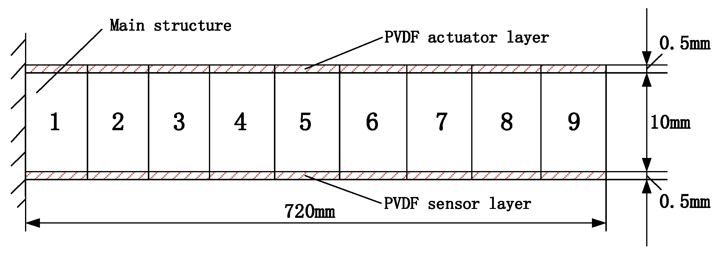
6. Numerical Example

Without loss of generality, we will control the first modal of a composite cantilever beam model, as shown in Figure 1. The length, width, and thickness of the main structure are 720 mm, 20 mm, and 10 mm, respectively. The mass density of the main structure is 7850 kg/m³ and the Young’s modulus is 210 GPa. Two thin layers of piezoelectric material (PVDF) are completely glued to the upper and lower surfaces to function as actuators and sensors. The parameters of the PVDF material are as follows: the thickness of each layer is 0.5 mm; the mass density is 1800 kg/m³; the Young’s modulus is 2 × 10⁹ Pa; the dielectric constant (polarization along the depth of the cantilever beam) is ${\epsilon }_{33}$= 0.1062 × 10⁻⁹; and the piezoelectric constant is e₃₁ = 0.046. The example will show that the location of the actuator affects the performance of the vibration control. Assuming that the actuating force for the actuator is 50% of the ideal control force, which means the actual gain is 50% of the ideal gain, the example also shows how to find out the optimal location and number of actuators required to control the vibration using the recursive design method. The example also demonstrates the impact of uncertain parameters on the structure using interval analysis.

Finite element equations for main structure are established using Euler–Bernoulli beam theory, as the ratio of length to height is 72. The main structure is divided into nine uniform beam elements with 10 nodes along the direction of length. Each node of this finite element model has two degrees of freedom, one translation and one rotation. The rotational degree of freedom is associated with the cross-section rotation. The left node is fixed and the others are free to move. Furthermore, we take the damping matrix $C=0.0012K$.

1.

The calculation of the optimal position of the control force that controls the first-order mode under the condition of realizable control.

From Equation (55) in Section 3.2, we see that the dimensionless sensitivity of the first-order modes of elements 1~9 is:

$${\tilde{\Omega }}_a=\left[1.0000, 0.6970, 0.4517, 0.2652, 0.1356, 0.0565, 0.0167, 0.0025, 6\times {10}^{-5}\right].$$

(95)

This means that when controlling the first-order mode, the optimal position of the control force is arranged on the first element $b_1$; the second optimal position is arranged on the second element $b_2$; the third optimal position is arranged on the third element $b_3$ …; the worst position is on the ninth element $b_9$.

The first two complex eigenvalues of the open-loop system are:

$${\lambda }_{10}=-6.1531-101.2676i,$$

(96)

$${\lambda }_{20}=-6.1531+101.2676i.$$

(97)

Suppose the first two complex eigenvalues of the open-loop system, ${\lambda }_{10}$ and ${\lambda }_{20}$, are configured on the poles ${\mu }_1$ and ${\mu }_2$ of the closed-loop system:

$${\mu }_1=-12.2600-120.0000i,$$

(98)

$${\mu }_2=-12.2600+120.0000i.$$

(99)

Adopt velocity and displacement feedback control, and the control force $u_1\left(t\right)$ should be applied at the optimal position $b_1$, the velocity feedback gain at $g_{c1}=\mathrm{166,860}$, and the displacement feedback gain at $g_{k1}=\mathrm{67,951}$. If $g_{k1}$ is the displacement feedback gain for each actuator, when the control force acts at element $b_i$, ${\tilde{\omega }}_{i1}$ is the first frequency of the close-loop system, and it can be sorted as ${\tilde{\omega }}_1$:

$$\begin{array}{ll}{\tilde{\omega }}_1=& [120.0000, 114.6481, 110.1239 \\ & 106.5570, 104.0065, 102.4169\\ & 101.6097, 101.3195, 101.2688]\end{array}.$$

(100)

Let $\mathsf{\Delta }{\omega }_{i1}={\tilde{\omega }}_{i1}-{\omega }_0$, where ${\omega }_0=101.2676$ rad/s is the first frequency of the open-loop system:

$$\begin{array}{ll}\mathsf{\Delta }{\omega }_1=& [18.7324, 13.3805, 8.8563\\ & 5.2894, 2.7389, 1.1493\\ & 0.3421, 0.0519, 0.0012]\end{array}.$$

(101)

Consider $\mathsf{\Delta }{\omega }_{11}=18.7324$ rad/s, $\mathsf{\Delta }{\omega }_{91}=0.0012$ rad/s, we have:

$$\frac{\mathsf{\Delta }{\omega }_{11}}{\mathsf{\Delta }{\omega }_{91}}=\frac{18.7324}{0.0012}=\mathrm{15,610}.$$

(102)

This means that the change in frequency of the control force in the optimal position $\mathsf{\Delta }{\omega }_{11}$ is 15,610 times that of the worst position $\mathsf{\Delta }{\omega }_{91}$. In other words, if the pole assignments are the same, the energy consumed when placing the actuator in the worst position is much greater than when placing the actuator in the optimal position. This illustrates the conclusions in Section 3.1. Therefore, it is important to select the position of the control force in the structural vibration control in practice.

2.

The optimal number and location of actuators.

Assume the actual gains provided by each actuator are ${\tilde{g}}_{c1\max }=0.5g_{c1}$ and ${\tilde{g}}_{k1\max }=0.5g_{k1}$, which means the actual force is 50% of the ideal control force. The optimal number and location of the actuators will be calculated using the recursive method proposed in Section 4.

• The first step:

When the actuator ${\tilde{u}}_1\left(t\right)$ is arranged in the optimal position $b_1$, we have

$${\mu }_{11}=-9.2065-111.0296i,$$

(103)

$${\mu }_{12}=-9.2065+111.0296i.$$

(104)

Compare ${\mu }_{11}$ and ${\mu }_{12}$ with ${\mu }_1$ and ${\mu }_2$, and we have −9.2065 > −12.2600 and 111.0296 < 120, an additional actuator is required and the second step is as follows:

• The second step:

The second actuator ${\tilde{u}}_2\left(t\right)$ is arranged in the optimal position $b_2$, and we have

$${\mu }_{21}=-11.3349-117.3545i,$$

(105)

$${\mu }_{22}=-11.3349+117.3545i.$$

(106)

Compare ${\mu }_{21}$ and ${\mu }_{22}$ with ${\mu }_1$ and ${\mu }_2$, and we have −11.3349 > −12.2600 and 117.3545 < 120, an additional actuator is still required and the third step is as follows:

• The third step:

A third actuator ${\tilde{u}}_3\left(t\right)$ is arranged in the optimal position $b_3$, and we have:

$${\mu }_{31}=-12.7140-121.2772i,$$

(107)

$${\mu }_{32}=-12.7140+121.2772i.$$

(108)

Compare ${\mu }_{31}$ and ${\mu }_{32}$ with ${\mu }_1$ and ${\mu }_2$, and we have −12.7140 < −0.1226 and 140.8476 > 140, and stop the calculation. Three actuators are needed to completely achieve the vibration control of the structure. In addition, they are arranged in positions $b_1$, $b_2$, and $b_3$.

3.

The effect of uncertain parameters on eigenvalues of the closed-loop control system.

Now, we have determined the number and location of the required actuators. We can substitute them into the system and discuss the impact of uncertain parameters on the structure to illustrate Section 5.

Suppose that the Young’s modulus $E^I=\left[E^c-\mathsf{\Delta }E,E^c+\mathsf{\Delta }E\right]$, mass density ${\rho }^I=\left[{\rho }^c-\mathsf{\Delta }\rho ,{\rho }^c+\mathsf{\Delta }\rho \right]$, and height $h^I=\left[h^c-\mathsf{\Delta }h,h^c+\mathsf{\Delta }h\right]$ are taken as interval parameters of the closed-loop system. Then, the upper and lower bounds of complex eigenvalues can be obtained according to interval stiffness, interval mass, and interval damping. $\mathsf{\Delta }\mathrm{Re}=\left|\mathrm{Re}\left(\mathsf{\Delta }\tilde{S}\right)\right|/\left|\mathrm{Re}\left({\tilde{S}}^c\right)\right|\%$ and $\mathsf{\Delta }\mathrm{Im}=\left|\mathrm{Im}\left(\mathsf{\Delta }\tilde{S}\right)\right|/\left|\mathrm{Im}\left({\tilde{S}}^c\right)\right|\%$ are the rates of change of the real and imaginary parts of eigenvalues, respectively. When the Young’s modulus of the main structure is $\mathsf{\Delta }E=\left(2\%,4\%,6\%\right)E^c$, the upper and lower bounds of complex eigenvalues of the first-order uncertain closed-loop system and the change rates of the real and imaginary parts of eigenvalues are respectively:

$$\begin{array}{c}{\mu }_{311}=\left[-12.8370,-12.5909\right]+\left[-122.1199i,-120.4286i\right], \mathsf{\Delta }\mathrm{Re}1=0.9678\%, \\ \mathsf{\Delta }\mathrm{Im}1=0.6973\%,\end{array}$$

(109)

$$\begin{array}{c}{\mu }_{312}=\left[-12.9601,-12.4679\right]+\left[-122.9568i,-119.5741i\right], \mathsf{\Delta }\mathrm{Re}2=1.9357\%, \\ \mathsf{\Delta }\mathrm{Im}2=1.3948\%,\end{array}$$

(110)

$$\begin{array}{c}{\mu }_{313}=\left[-13.0832,-12.3448\right]+\left[-123.7880i,-118.7133i\right], \mathsf{\Delta }\mathrm{Re}3=2.9039\%, \\ \mathsf{\Delta }\mathrm{Im}3=2.0926\%.\end{array}$$

(111)

When the mass density of the main structure is $\mathsf{\Delta }\rho =\left(2\%,4\%,6\%\right){\rho }^c$, the upper and lower bounds of complex eigenvalues of the first-order uncertain closed-loop system and the change rates of the real and imaginary parts of the eigenvalues are:

$$\begin{array}{c}{\mu }_{311}=\left[-12.9734,-12.4647\right]+\left[-122.5085i,-120.0823i\right], \mathsf{\Delta }\mathrm{Re}1=1.9998\%, \\ \mathsf{\Delta }\mathrm{Im}1=1.0001\%,\end{array}$$

(112)

$$\begin{array}{c}{\mu }_{312}=\left[-13.2437,-12.2250\right]+\left[-123.7780i,-118.9221i\right], \mathsf{\Delta }\mathrm{Re}2=3.9998\%, \\ \mathsf{\Delta }\mathrm{Im}2=2.0008\%,\end{array}$$

(113)

$$\begin{array}{c}{\mu }_{313}=\left[-13.5255,-11.9943\right]+\left[-125.0879i,-117.7948i\right], \mathsf{\Delta }\mathrm{Re}3=6.0000\%, \\ \mathsf{\Delta }\mathrm{Im}3=3.0027\%.\end{array}$$

(114)

When the height of the main structure $\mathsf{\Delta }h=\left(2\%,4\%,6\%\right)h^c$, the upper and lower bounds of complex eigenvalues of the first-order uncertain closed-loop system and the change rates of the real and imaginary parts of the eigenvalues are:

$$\begin{array}{c}{\mu }_{311}=\left[-13.0813,-12.3516\right]+\left[-123.3007i,-119.2539i\right], \mathsf{\Delta }\mathrm{Re}1=2.8691\%, \\ \mathsf{\Delta }\mathrm{Im}1=1.6684\%,\end{array}$$

(115)

$$\begin{array}{c}{\mu }_{312}=\left[-13.4535,-11.9942\right]+\left[-125.3242i,-117.2306i\right], \mathsf{\Delta }\mathrm{Re}2=5.7345\%, \\ \mathsf{\Delta }\mathrm{Im}2=3.3368\%,\end{array}$$

(116)

$$\begin{array}{c}{\mu }_{313}=\left[-13.8307,-11.6417\right]+\left[-127.3478i,-115.2075i\right], \mathsf{\Delta }\mathrm{Re}3=8.5936\%, \\ \mathsf{\Delta }\mathrm{Im}3=5.0052\%.\end{array}$$

(117)

These results show that when uncertain parameters increase, the change rate of eigenvalues increases, that is, the error of eigenvalues increases with the increase in uncertain parameters. For example, when the Young’s modulus of the structure is $\mathsf{\Delta }E=2\%E^c$, the change rates of the real and imaginary parts of the first eigenvalue are 0.9678% and 0.6973%, respectively. When the Young’s modulus of the main structure is $\mathsf{\Delta }E=6\%E^c$, the change rates of the real part and imaginary part of the first eigenvalue are 2.9039% and 2.0926%, respectively. When the height of the main structure is $\mathsf{\Delta }h=2\%h^c$, the change rates of the real part and imaginary part of the first eigenvalue are 2.8691% and 1.6684%, respectively. When the height of the main structure is $\mathsf{\Delta }h=6\%h^c$, the change rates of the real part and imaginary part of the first eigenvalue are 8.5936% and 5.0052%, respectively. In addition, on the whole, the uncertainty of the height of the structure has a greater influence on the eigenvalues than the Young’s modulus or mass density.

7. Conclusions

• This paper discusses the measurement of modal controllability of intelligent structures, deduces a control matrix singular value sensitivity formula, and determines the optimal position of piezoelectric actuators for an intelligent structure. In a numerical example, when the sizes of the actuators are exactly the same and the displacement feedback gains are exactly the same, it is very important to select the location of actuators in a structural vibration control;
• When a single actuator is applied, the feedback gain matrix is calculated using the receptance method, and the ideal control force of actuator is calculated. When the control force required for complete controllability of the structure is much higher than the actual force of the actuator, a single-input control cannot fully control the structure, and a multi-input control is needed for the purpose of vibration control. The recursive design method of a modal controller is introduced to study the optimal number and location of the actuators;
• The change rate of eigenvalues of a closed-loop control system increases with the increase in the uncertain parameters. Uncertain parameters are expressed as intervals. A method is proposed to solve the upper and lower bounds of the eigenvalues of a closed-loop control system with uncertain parameters using perturbation theory and interval analysis and is illustrated with a numerical example.

In conclusion, this paper solves the problem of the optimal number and position of actuators when the control force is greater than the range of the actuator’s execution force. The structure can be fully controllable by increasing the number of actuators. Interval theory is used to discuss the effect of uncertain parameters on eigenvalues of closed-loop control systems.

References

1. Lin, Y.K. Probabilistic Theory of Structural Dynamics; McGraw-Hill: New York, NY, USA, 1967. [Google Scholar]
2. Dief, A.S. Sensitivity Analysis in Linear Systems; Springer: Berlin, Germany, 1986. [Google Scholar]
3. Lindberg, H.E. Dynamic response and buckling failure measures for structures with bounded and random imperfections. Trans. ASME J. Appl. Mech. 1991, 58, 1092–1094. [Google Scholar] [CrossRef]
4. Ganzerli, S.; Pantelides, C.P. Load and resistance convex models for optimum design. Struct. Optim. 1999, 17, 259–268. [Google Scholar] [CrossRef]
5. Moore, R.E. Methods and Applications of Interval Analysis; Society for Industrial and Applied Mathematics: Philadelphia, PA, USA, 1979. [Google Scholar]
6. Dessombz, O.; Thouverez, F.; Laine, J.P.; Jezequal, L. Analysis of mechanical system using interval computations applied to finite element methods. J. Sound Vibr. 2001, 239, 949–968. [Google Scholar] [CrossRef] [Green Version]
7. Mori, T.; Kokame, H. Convergence property of interval matrices and interval polynomials. Int. J. Contr. 1987, 45, 481–484. [Google Scholar] [CrossRef]
8. Rachid, A. Robustness of discrete systems under structural uncertainties. Int. J. Contr. 1989, 50, 1563–1566. [Google Scholar] [CrossRef]
9. Wonham, W.M. On pole assignment in multi-input controllable linear system. IEEE Trans. Autom. Control 1967, 12, 660–665. [Google Scholar] [CrossRef] [Green Version]
10. Datta, B.N.; Elhay, S.; Ram, Y.M. Orthogonality and partial pole assignment for the symmetric difinite quadratic pencil. Linear Algebra Its Appl. 1997, 257, 29–48. [Google Scholar] [CrossRef]
11. Duan, G.R. Parametric eigenstructure assigment in second-order descriptor linear systems. IEEE Trans. Autom. Control 2004, 49, 1789–1795. [Google Scholar] [CrossRef]
12. Mottershead, J.E.; Ram, Y.M. Receptance method in active vibration control. AIAA J. 2007, 3, 562–567. [Google Scholar]
13. Ram, Y.M.; Mottershead, J.E. Multiple-input active vibration control by partial pole placement using the method of receptances. Mech. Syst. Signal Process. 2013, 40, 727–735. [Google Scholar] [CrossRef]
14. Mokrani, B.; Palazzo, F.; Mottershead, J.E.; Fichera, S. Multiple-input multiple-output experimental aeroelastic control using a receptance-based method. AIAA J. 2019, 7, 3066–3077. [Google Scholar] [CrossRef]
15. Tsai, S.H.; Ouyang, H.; Chang, J.Y. Identification of torsional receptances. Mech. Syst. Signal Process. 2019, 126, 116–136. [Google Scholar] [CrossRef]
16. Gao, X. Research on Theory and Algorithm of Local Vibration Control of Structure. Ph.D. Thesis, Jilin University, Changchun, China, 2009. [Google Scholar]
17. Chen, S.; Cao, Z. A new method for determining locations of the piezoelectric Sensor/Actuator for vibration control of intelligent structures. J. Intell. Mater. Syst. Struct. 2000, 11, 108–115. [Google Scholar] [CrossRef]
18. Lim, T.W. Actuator/sensor placement for modal parameter identification of flexible structures. Modal Anal. Int. J. Anal. Exp. Modal Anal. 1993, 1, 1–13. [Google Scholar]
19. Schulz, G.; Heimbold, G. Dislocated actuator/sensor positioning and feedback design for flexible Structures. J. Guid. Control. Dyn. 1982, 6, 361–367. [Google Scholar] [CrossRef]
20. Rao, S.S.; Pan, T. Optimal placement of actuators in actively controlled structures using genetic algorithm. AIAA J. 1991, 5, 942–943. [Google Scholar] [CrossRef]
21. Levine, W.S.; Athans, M. On the determination of the constant output feedback gains for linear multivariable systems. Trans. Autom. Control 1970, 15, 44–48. [Google Scholar] [CrossRef]
22. Kang, Y.K.; Park, H.C.; Hwang, W.; Han, K.S. Optimum placement of piezoelectric sensor/actuator for vibration control of laminated beams. AIAA J. 1996, 9, 1921–1926. [Google Scholar] [CrossRef]
23. Choe, K.; Baruh, H. Actuator placement in structural control. J. Guid. Control Dyn. 1991, 1, 40–46. [Google Scholar] [CrossRef]
24. Baruh, H.; Merovitch, L. On the placement of actuators in the control of distributed-parameter systems. AIAA J. 1981, 611–618. [Google Scholar] [CrossRef]
25. Chen, S.H. Matrix Perturbation Theory in Structural Dynamics; Science Press: Beijing, China, 2007. [Google Scholar]
26. Zienkiewicz, O.C.; Taylor, R.L. The Finite Element Method; Butterwort-Heinemann: Oxford, UK, 2000. [Google Scholar]
27. Craig, R.R. Structural Dynamics: An Introduction to Computer Methods; Wiley: New York, NY, USA, 1981. [Google Scholar]
28. Rong, B.; Rui, X.; Lu, K.; Tao, L.; Wang, G.; Ni, X. Transfer matrix method for dynamics modeling and independent modal space vibration control design of linear hybrid multibody system. Mech. Syst. Signal Process. 2018, 104, 589–606. [Google Scholar] [CrossRef]
29. Neto, M.A.; Ambrósio, J.A.C.; Roseiro, L.M.; Amaro, A.; Vasques, C.M.A. Active vibration control of spatial flexible multibody systems. Multibody Syst. Dyn. 2013, 30, 13–35. [Google Scholar] [CrossRef]
30. Tzou, H.S.; Tseng, C.I. Distributed piezoelectric sensor/actuator design for dynamic measurement/control of distributed parameter system: A piezoelectric finite element approach. J. Sound Vib. 1990, 138, 17–34. [Google Scholar] [CrossRef]
31. Preumont, A. Mechatronics Dynamics of Electromechnical and Piezoelectric Systems; Springer: Dordrecht, The Netherlands, 2006. [Google Scholar]
32. Mokrani, B.; Batou, A. The minimum norm multi-input multi-output receptance method for partial pole placement. J. MSSP 2019, 129, 437–448. [Google Scholar] [CrossRef]
33. Yao, G.; Gao, X. Controllability of regular systems and defective systems with repeated eigenvalues. J. Vib. Control. 2010, 17, 1574–1581. [Google Scholar]
Figure 1. Composite cantilever beam structure.
Actuators 09 00031 g001