Optimization of Ultrasonic Acoustic Standing Wave Systems

Abstract

Ultrasonic acoustic standing wave systems find use in many industrial applications, such as sonochemical reactions, atomization of liquids, ultrasonic cleaning, and spray dry. In most applications, highest possible sound pressure levels are needed to achieve optimum results. Until now, the atomization of liquids is limited to fluids with low viscosity, as systems generating sufficient sound pressure for atomizing fluids with higher viscosities are often not marketable due to their low throughput or high costs. For the production of polymer or metal powders or the dispensing of adhesives, highest sound pressures should be achieved with systems in suitable size, with good efficiency and at low cost but without contamination of sonotrodes and reflectors by the dispersed media. An alternative to the use of more powerful transducers is increasing the intensity of the acoustic standing wave field by optimizing the boundary conditions of the acoustic field. In most existing standing wave systems a part of the radiating sound waves does not contribute to the process, as the waves spread into the wrong direction or wipe themselves out due to interference. In order to obtain maximum sound pressure amplitudes in the standing wave field, all waves should be trapped between the sonotrode and the reflector. In addition, the resonance condition should be met for all radiated waves. These conditions can be fulfilled by optimizing the shapes of sonotrode and resonator as well as the distance between them. This contribution reports on a model, which is able to simulate the sound field between a transducer surface and a reflector. Using a linear finite-element model, the boundary conditions of the standing wave system are optimized. Sound pressure levels of the standing wave field are calculated for different shapes of reflectors and boundary conditions like the distance between the transducer and the reflector. The simulation results are validated by sound-field measurements via refracto-vibrometry and a microphone. Finally, optimization guidelines for the generation of high-intensity acoustic standing wave fields are shown and verified by measurements.

1. Introduction

Every vibrating system emits sound waves to its environment, which can be disturbing but can also be used to improve processes like cleaning, chemical reactions, or dispersing of fluids and powders. To generate ultrasonic waves, typically piezoelectric bolt-clamped Langevin transducers are used [1,2,3,4,5], which can generate high power ultrasonic radiation at electrical power of up to a few kilowatts. As in any other vibrating system, the ultrasonic transducer principally emits a traveling wave. Using a reflector, which is placed across from the sonotrode, a standing wave is generated. At resonant distance between the reflector and the transducer, radiated and reflected waves are optimally superimposed, resulting in higher sound pressure amplitudes. As shown in Equation (1), the resonant distance of a one-dimensional sound wave between two reflectors is an integer multiple of half the wavelength

$$L=n\lambda /2,$$

(1)

with the wavelength of the sound wave $\lambda$ and a whole number n. Equation (1) is derived from the calculation of the resonant length of a pipe closed at both ends [6].

There are some approaches to maximize sound pressure. A simple solution is the increase of vibration amplitudes of the transducer, which might lead to damage or at least to reduction of lifetime. High sound pressures are also achieved at a minimum distance between transducer and reflector, which ideally equals $L=\lambda /2$. However, the volume of the sound field is very small in this case and might be too small for most processes. Another method is the use of two oppositely arranged transducers [7]. However, the generation of a standing wave requires an exact tuning of frequency, phase and amplitude of both transducers, which requires a complicated control and high manufacturing accuracy.

In most technical systems sound waves are emitted spherically, even though the sound sources vibrate uniaxially [8]. Due to dispersion of the sound waves, the pressure amplitude of standing wave systems in the far field drops rapidly with increasing distance from the transducer. Similarly, the maximum pressure at the resonant distances (see Equation (1)) decreases with increasing number of n.

When a plain reflector is used, as depicted in Figure 1, only sound waves, that are roughly parallel to the rotation axis, are reflected back to the transducer and contribute to the standing wave field. Other sound waves might still reach the reflector but do not reach the transducer after reflection. In addition, the waves have different path lengths, depending on the radiation angle. The standing wave condition (see Equation (1)) is fulfilled only for waves near the rotation axis. To overcome these issues, the geometries of transducer and reflector have to be optimized so that the highest possible sound pressure is achieved in the sound field.

In the following sections, a model is presented, which is used for the model-based optimization. Modeling results for optimized geometries are shown, discussed, and validated by measurements on an experimental setup of a standing wave system.

2. Model Setup

The basic requirement to a model for model-based optimization is sufficient accuracy at short calculation time. The model is implemented in ANSYS Mechanical. Acoustic properties and acoustic boundary conditions are defined using a linear acoustic modeling approach as described in [9,10]. To reduce the complexity of the model, only a radial plane of the axially symmetric sound field is modeled [11]. As the wavelength in air is about 16 mm at the operating frequency of 21.4 kHz, a square elements mesh with size of 1 by 1 mm is set, which is completely sufficient for accurate simulation results. Sound absorption effects in air have been neglected.

Figure 2 shows the finite element model of the standing wave system. The dimensions of the model have been adapted from an existing standing wave system. The transducer’s output surface (diameter 30 mm) is assumed to vibrate at a frequency of $f=21.4$ kHz and vibration amplitude of $\widehat{x}=19$ $\mathsf{\mu }$m (excitation for sound field). A reflector with a diameter of 85 mm is placed at a distance L in opposition to the transducer’s output surface. Transducer and reflector are modeled by means of acoustically rigid boundaries (leading to total reflection of incident acoustic waves). All other boundaries of the acoustic chamber have been modeled as non-reflective-surfaces to represent an open space. Here, ANSYS’ simplified “impedance boundary” was used. Further details are described in the manual of ANSYS Mechanical APDL [9,10].

The simulation result of the model is the sound pressure level at every point in the rotationally symmetric plane. The sound pressure level

$$L_p=20lo{g}_{10}(p_{rms}/p_0)$$

(2)

is calculated from the RMS-value of the sound pressure $p_{rms}$ and the reference sound pressure $p_0=20$ $\mathsf{\mu }$Pa.

Simulation results for the standing wave system with a plain reflector are shown in Figure 3. The pictures show the sound field pattern for two different resonant distances. At a distance of $L=17$ mm, the sound pressure level is up to 176 dB. At the greater distance of $L=66.4$ mm, the entire sound field shows a reduced sound pressure level with maximum levels of 163 dB. In terms of sound pressure, this means a reduction by the factor 4.

Figure 4 shows the maximum sound pressure level in the sound field of the standing wave system with plain reflector over varying distance L. The resonant distances L fit quite well with the theoretical approach in Equation (1). The sound pressure levels at resonant distances drop with increasing number of n, which is caused by “losses” due to the dispersion of sound waves (see Figure 1).

3. Model Based Optimization

To achieve maximum sound pressures by only improving geometrical dimensions of the sound field, it must be ensured that the standing wave condition is fulfilled for all sound waves (see Equation (1)). Furthermore, it should be ensured that less sound waves are dissipated from the sound field.

In order to fulfill the standing wave condition for all radiated waves, it must be ensured that all wave paths comply with the standing wave condition, as shown in Equation (1). It must also be ensured that the waves reach the reflector as orthogonally as possible, so that they are reflected back to the transducer.

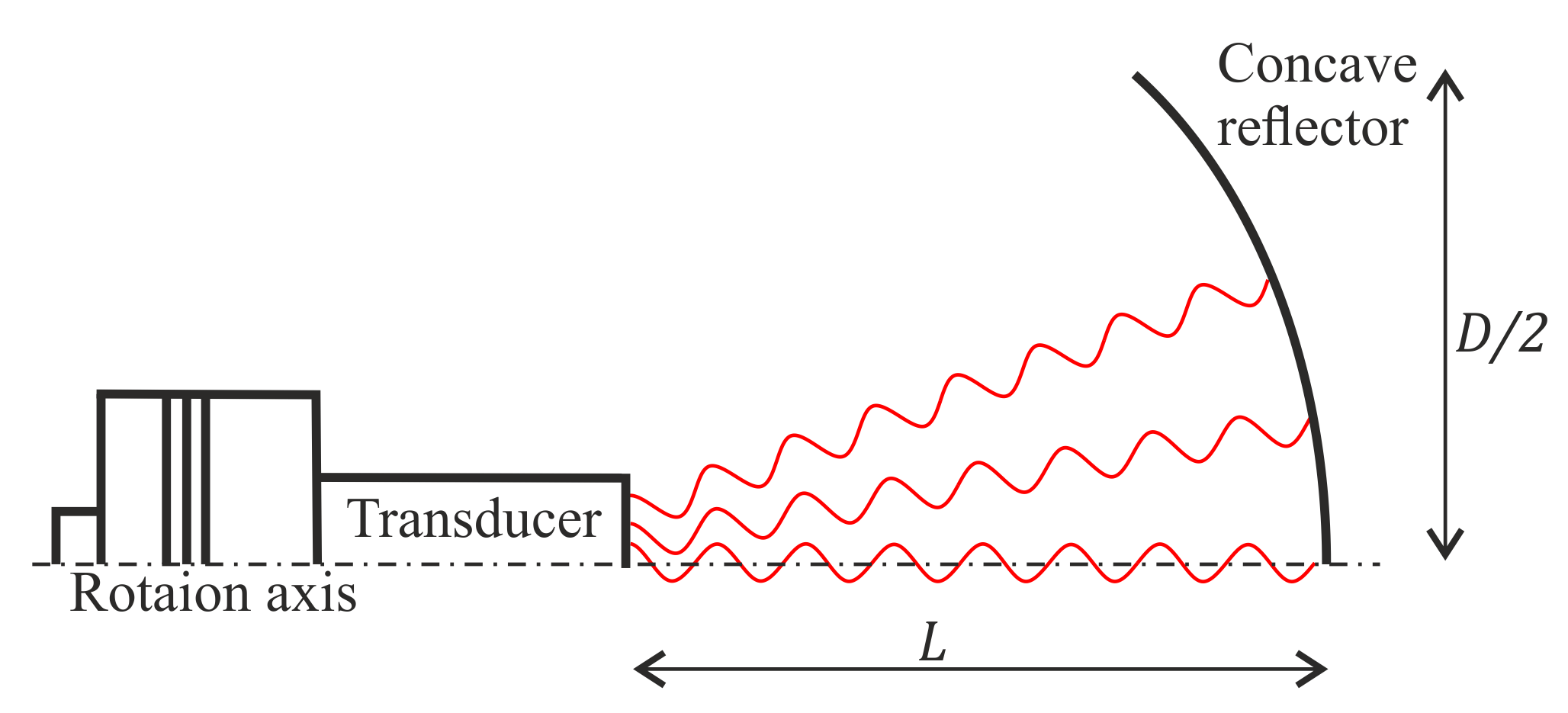
Figure 5 shows an approach of an improved standing wave system with a concave reflector [4]. The transducer is still piston-shaped and therefore has a planar radiation surface. When assuming that the transducer emits a spherical wave, the optimal radius for the reflector would be $R=L$. Accordingly, the dimensions of the reflector must always be adapted to the distance L. Both goals, the standing wave condition and orthogonal reflection at the reflector, are achieved by the same geometric modifications, which greatly simplifies the system optimization.

Figure 6 shows the maximum sound pressure level of the standing wave system with a concave reflector with a radius of $R=72$ mm and a diameter of $D=85$ mm over the distance L. In comparison, the diagram also shows the maximum sound pressure level of a system with plain reflector at the same distance. The maximum sound pressure of the system with concave reflector is higher than the one with plain reflector for every resonant distance. In contrast to the system with plain reflector, the maximum sound pressure level of the system with concave reflector does not decrease steadily. In addition to the optimum at $L\approx \lambda /2$, the system with concave reflector has a second local optimum at a distance of $L\approx R$. 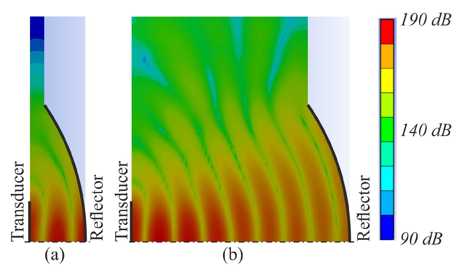The optimum does not appear at exactly $L=R$, because the transducer is not an ideal spherical radiator. The sound field patterns for two distances, $L_1$ and $L_2$, are shown in Figure 7. Compared to the sound field patterns of the system with a plain reflector (see Figure 3), overall higher sound pressure levels are achieved. The maximum sound pressure level at the distance of $L=17.4$ mm is 185 dB. At a greater distance of $67.8$ mm, the maximum sound pressure level is even higher, reaching 188 dB.

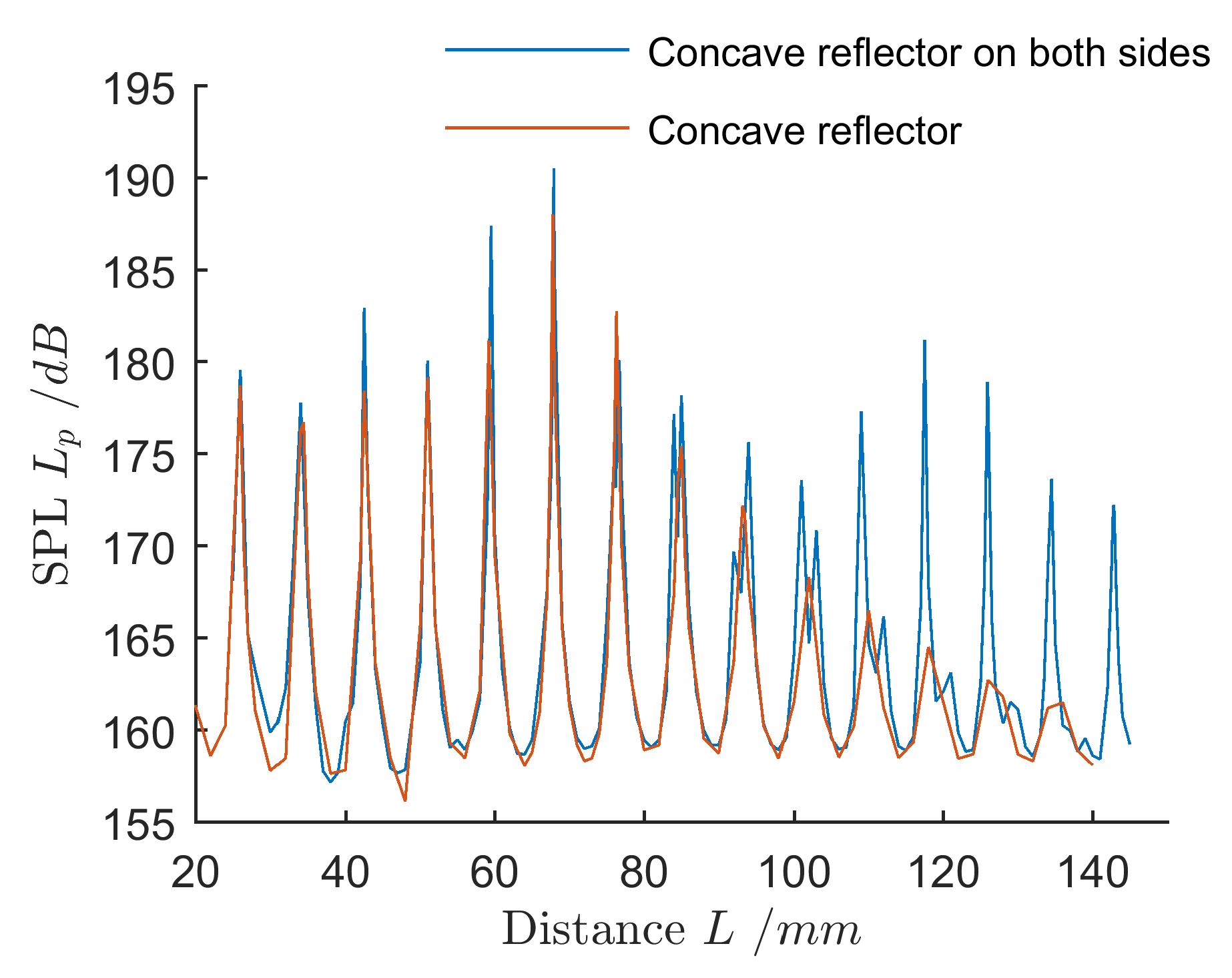
To further reduce the loss of soundwaves, a second reflector was placed at the side of the transducer. Figure 8 shows the maximum sound pressure levels over varying distance L for a standing wave system with concave reflectors on both sides in comparison to the system with a single concave reflector.

For distances below the second optimum at $L<=67.8$ mm, both systems do not show great differences in the maximum sound pressure level. At distances above the second optimum, the maximum sound pressure levels of the system with a single concave reflector rapidly drop with higher distance. However, in the system with concave reflector on both sides, the sound pressure level reaches a third optimum at a distance of $L=117.5$ mm. Although the maximum sound pressure level at this distance is somewhat smaller than at the second optimum at a distance of $L=67.8$ mm, the volume of the sound field is much bigger.

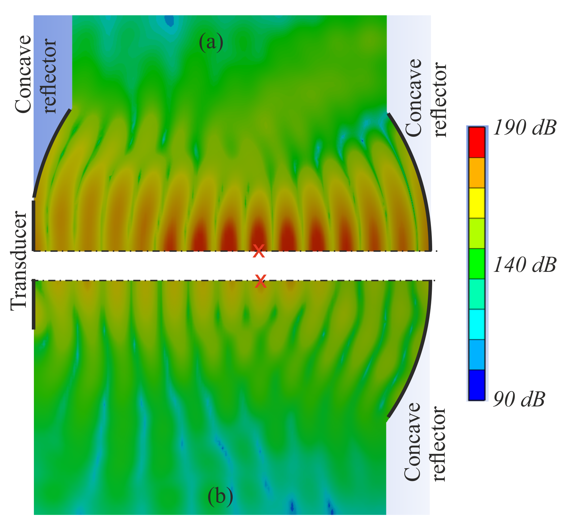
Figure 9 shows the sound field pattern of the standing wave system with concave reflector on both sides at a resonant distance of $L=117.5$ mm (a) and for comparison the sound field of a standing wave system with single concave reflector at the nearest resonant distance of $L=118$ mm (b). Figure 9a clearly shows the focusing effect of both reflectors, reaching a maximum sound pressure level of 181 dB. Compared to the system with single concave reflector (see Figure 9b), higher sound pressure levels with greater expansion are achieved. Furthermore, with the concave reflectors on both sides, the maximum sound pressure level is in the middle of the sound field and thus far away from the reflectors and the transducer. This might be an important advantage for the atomizing processes, where the dispersed medium tends to pollute the reflectors.

4. Nonlinear Effects

Regarding the model results (see Figure 4, Figure 6 and Figure 8), it is noticeable that extremely high sound pressures occur, especially at the optimal distances. These cannot be achieved by any real system.

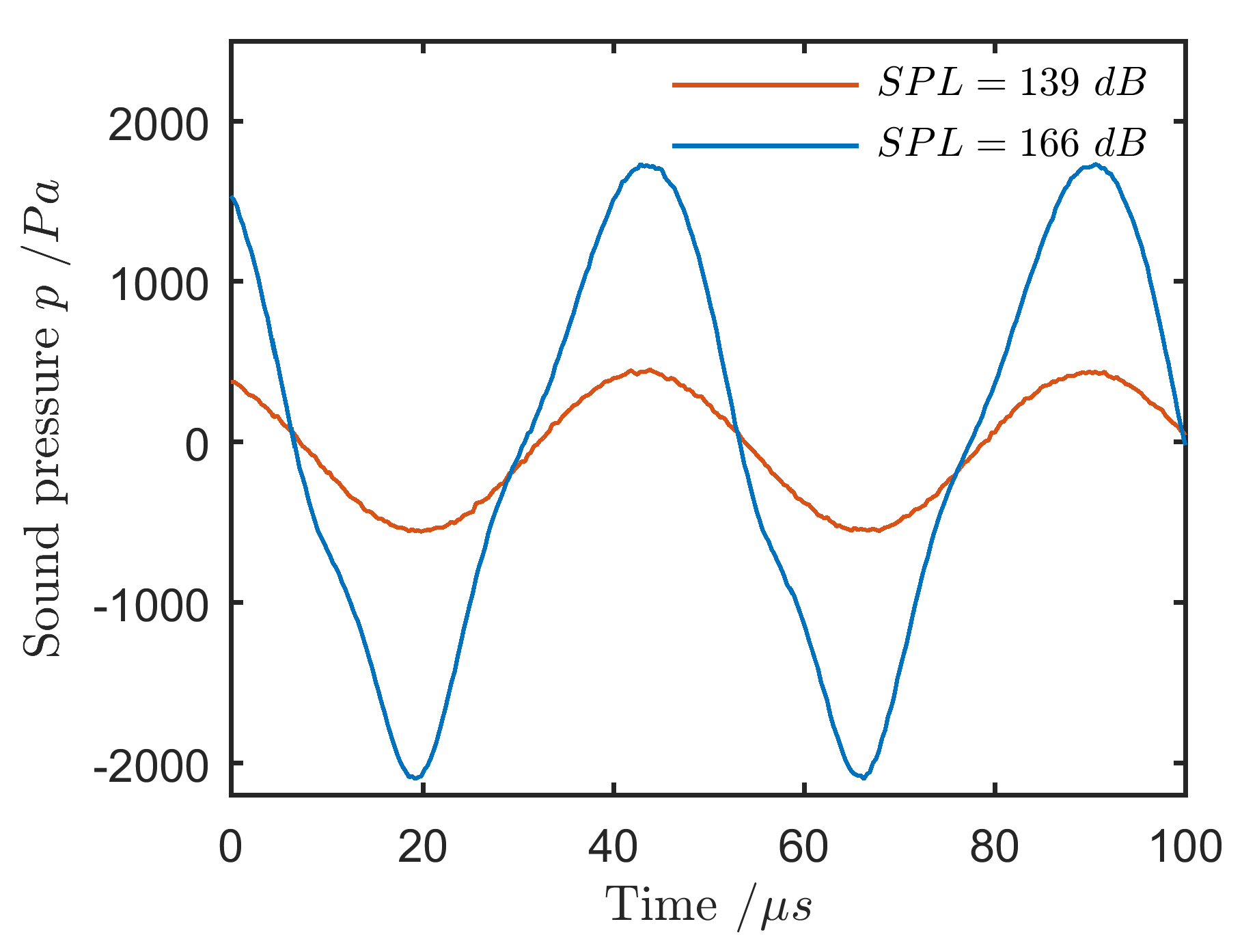
Figure 10 shows measurements of traveling sound waves (no reflection) at different sound pressure levels. At the rather low sound pressure level of 139 dB, the sound wave is sinusoidal like in the initial state. However, at the higher sound pressure level of 166 dB, the sound wave is more likely a sawtooth-shape.

This nonlinearity in sound fields at high sound pressure levels is already known and profoundly described in literature [12]. The main reason for the nonlinear effects is that the sound propagation velocity does not only depend on the infinitesimal sound velocity constant but also on the local velocity of the gaseous particles. In the compressional phase of the sound wave, for example, the sound propagation velocity becomes supersonic, i.e., greater than the sound velocity constant [12,13]. The sound wave thus distorts in the time domain and therefore generates new frequency components in the frequency domain. The new higher-harmonics always have a frequency of a multiple of the fundamental harmonic. Since the absorption of ultrasound increases with the frequency, the amplitude of the entire sound wave is decreased.

Whereas a sawtooth shape is obtained in the case of a traveling wave at high sound pressures (see Figure 10), a triangular shape is formed in standing wave fields by superimposing waves going back and forth. These effects become relevant for sound pressure levels of 140 dB and higher [12]. Since much higher sound pressure levels are addressed for technical processes, these nonlinear effects must be considered within the process optimization. Nevertheless, as the wavelength is not affected by the nonlinear effects, a linear model is sufficient for optimizing the geometry of the sound field. Calculated maximum sound pressure levels will be overestimated but can be calibrated by measurements.

5. Experimental Validation

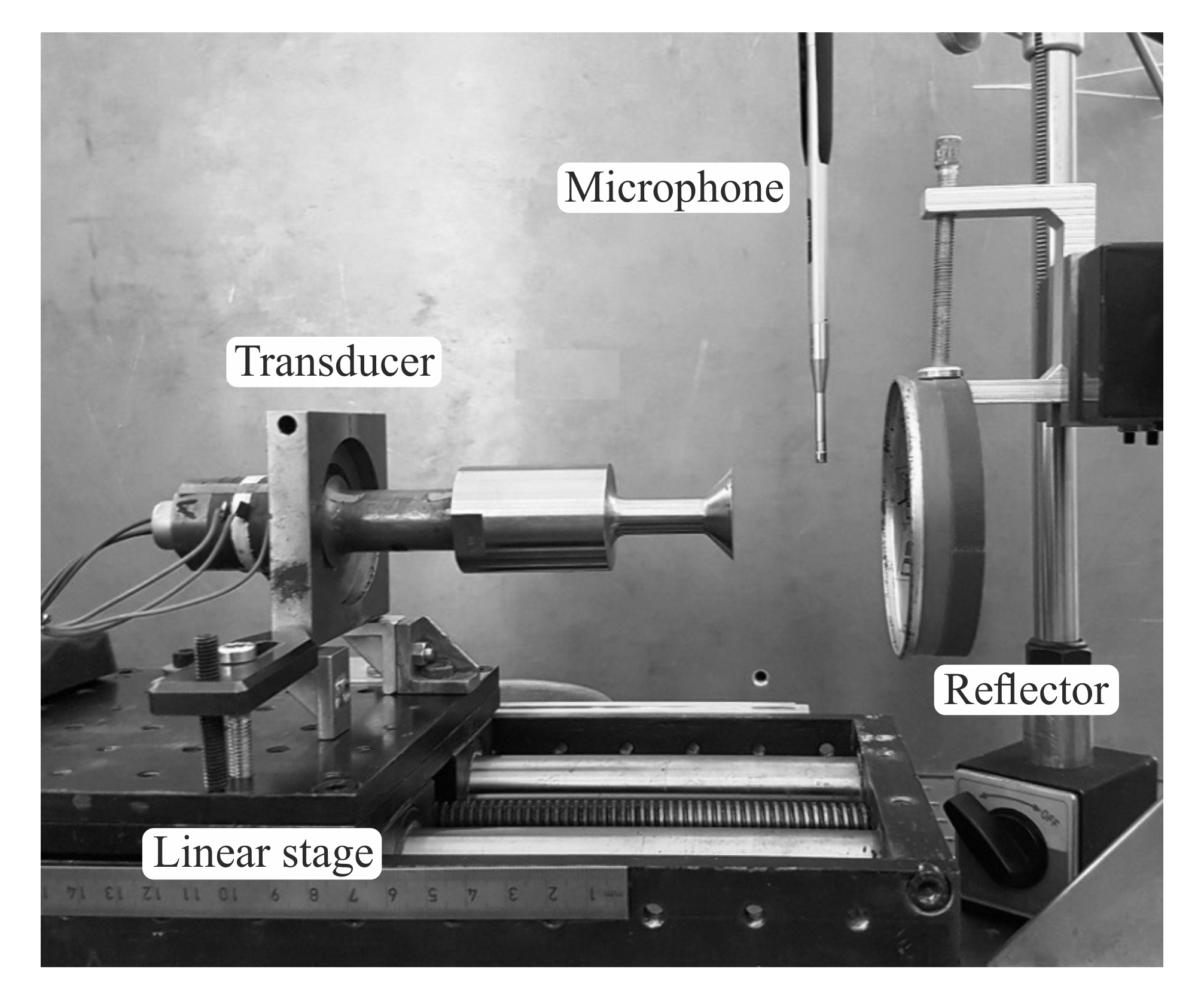
To validate the modeling and optimization results, an experimental setup was built, consisting of an ultrasonic transducer with planar radiation surface, which is driven at a frequency of $f=21.4$ kHz and an amplitude of $\widehat{x}=19$ $\mathsf{\mu }$m [11]. Figure 11 shows the transducer, mounted on a linear table and a concave reflector with a radius of $R=72$ mm and a diameter of $D=85$ mm (Wall thickness: $0.4$ mm, Material: Steel). The distance between transducer front and reflector can be adjusted continuously to distances L between 0 and 200 mm.

Sound pressures were measured using two different measurement principles. For measuring sound pressure at single points in the sound field, a microphone (Brüel&Kjaer, Type 4138, pressure range: 52–168 dB, see Figure 11) and a pressure sensor (ALTHEN, Model EPIH-11, pressure range: 1 bar) were used. Instead of measuring the complete sound field pattern, refracto-vibrometry with a scanning laser-doppler-vibrometer (Polytec, PSV500) was used [14,15], which results in patterns of a virtual velocity that is proportional to the sound pressure.

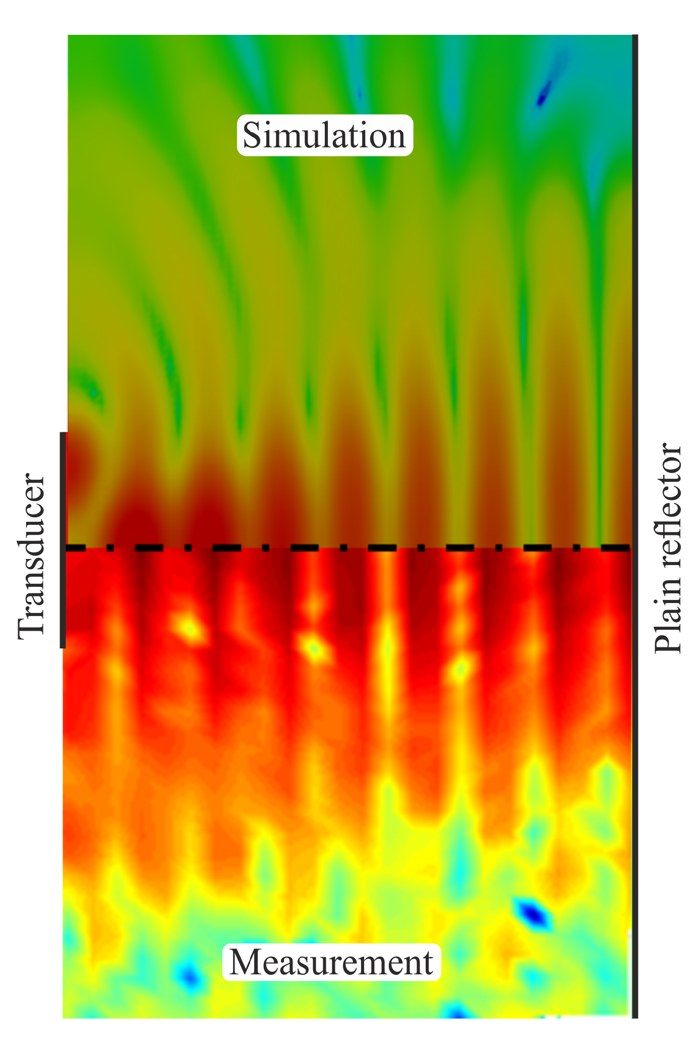
Figure 12 shows the patterns of the standing wave system with plain reflector determined by simulations and experiments. Apart from small differences near the transducer, the patterns of simulation and experiment are qualitatively identical.

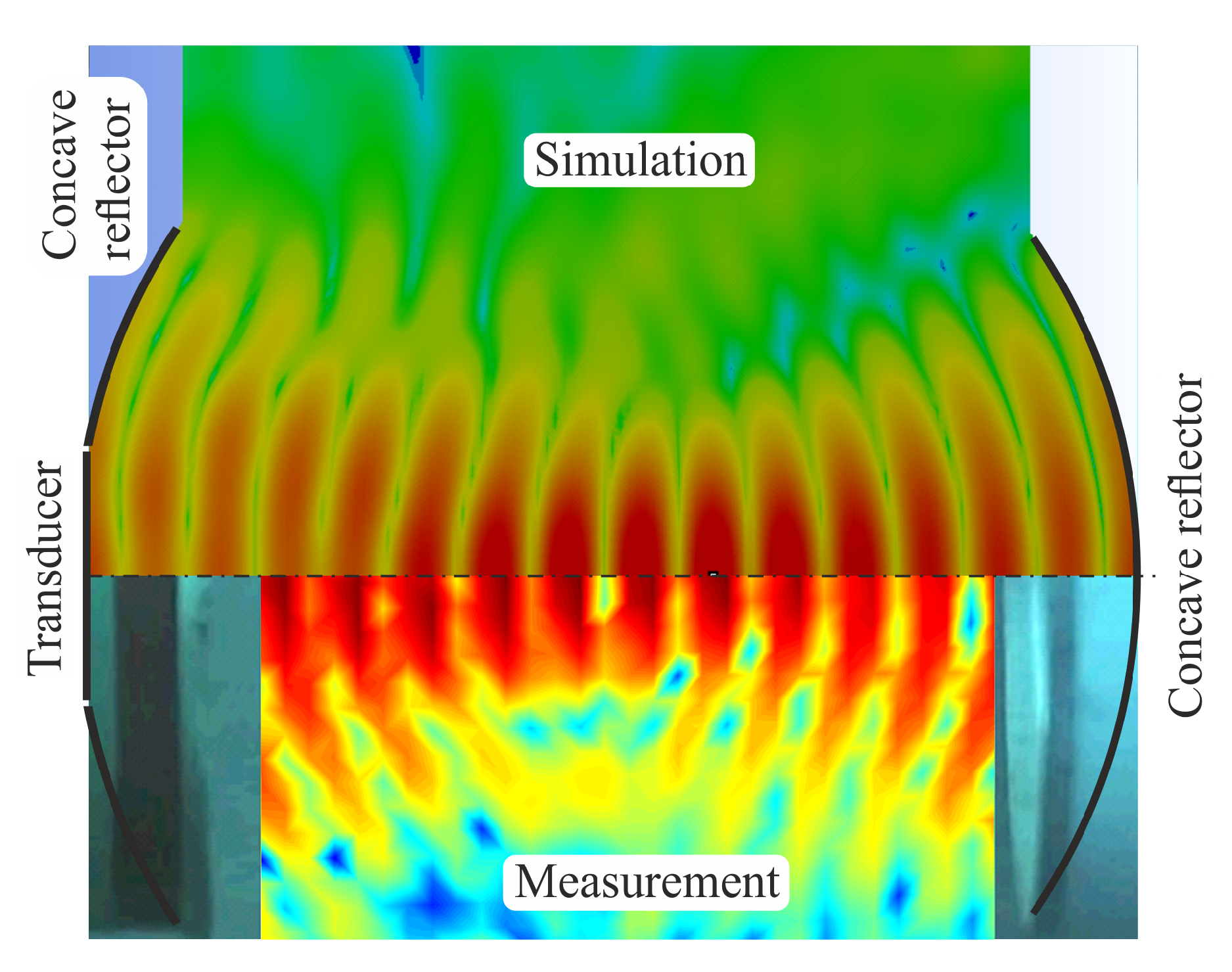
For the standing wave system with concave reflector (see Figure 13) and with reflectors on both sides (see Figure 14), simulation and experimental results are in very good agreement as well.

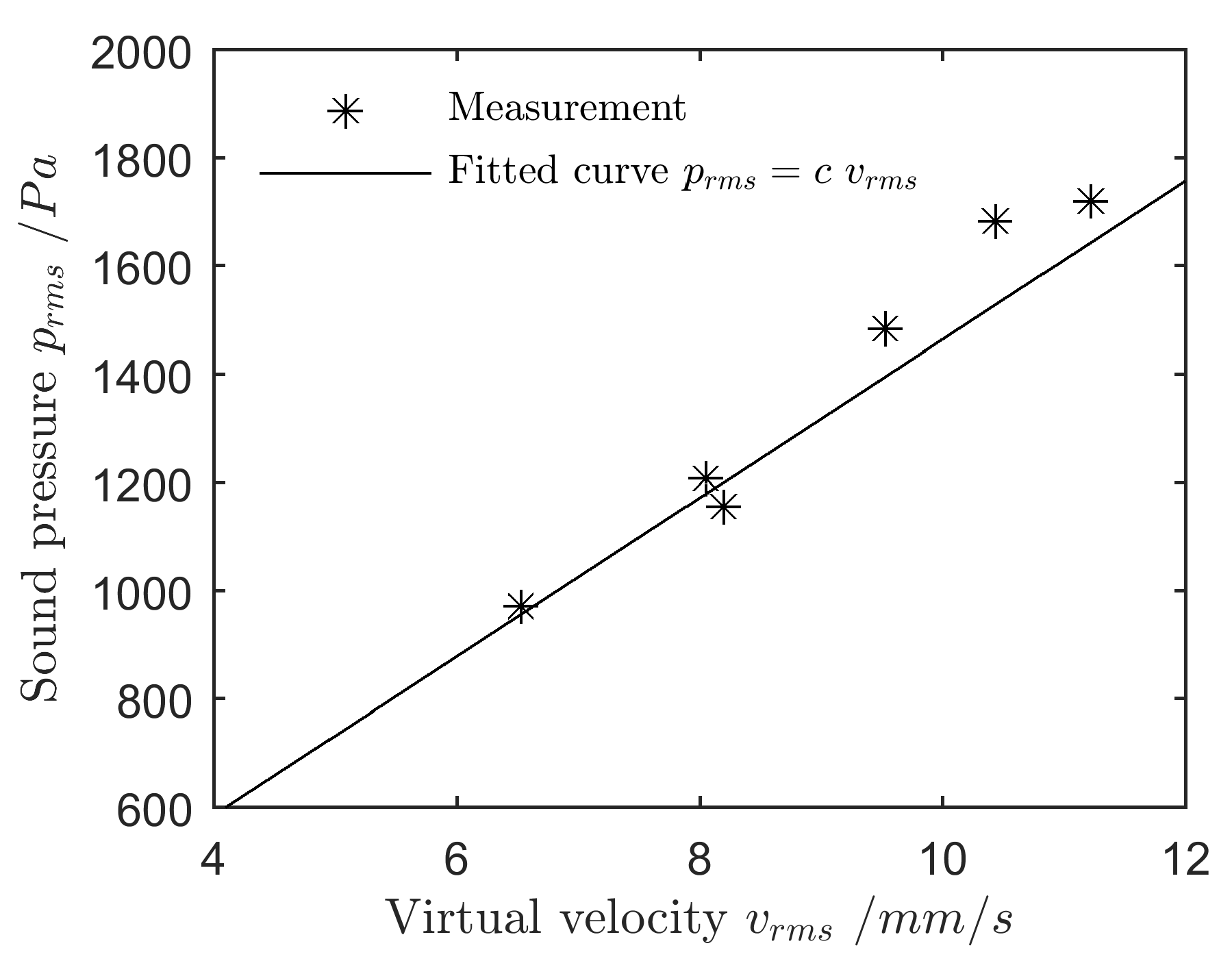
The previous validation only referred to the comparison of the field pattern. For a validation of qualitative results, the SLDV measurements should be scaled. For this purpose, a measurement of the field pattern (virtual velocity amplitude $\widehat{v}$) and measurements of the sound pressure level $L_p$ (using the microphone) at single points are combined. The measurements with the microphone must be taken with caution, as if the microphone is held into the sound field, sound field pattern and sound pressures can be affected. It is therefore advisable to do the microphone measurements in the outer area of the sound field. At the points with measurement values of both virtual velocity and sound pressure, a scaling factor $c=v_{rms}/p_{rms}$ is calculated, which is then used to scale all other points of the SLDV measurement. The scaling factor c was determined at different sound pressures $p_{rms}$. Corresponding measurements of sound pressure $p_{rms}$ and virtual velocity $v_{rms}$ (see Figure 15) show a linear relationship.

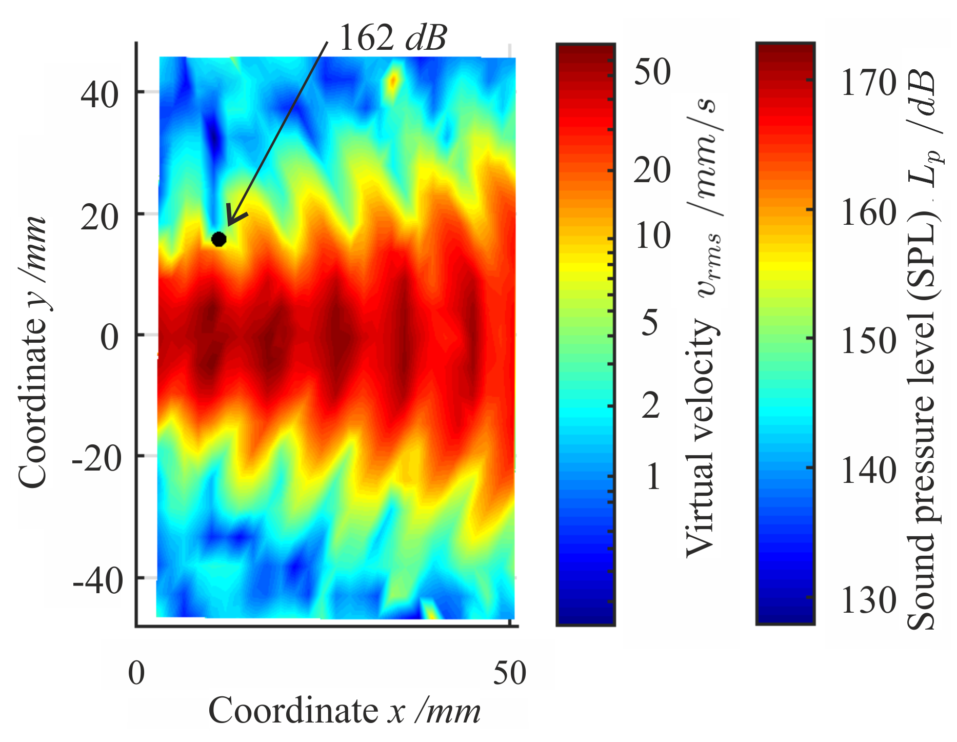
Using the scaling factor, the sound pressure level in the whole sound field is calculated. Figure 16 shows the sound field of the standing wave system with concave reflector after scaling to the logarithmic sound pressure level (SPL).

Using the shown method, the maximum sound pressure level of the standing wave system with single concave reflector at excitation amplitude of $\widehat{x}=19$ $\mathsf{\mu }$m and a frequency of $21.4$ kHz was estimated to be at 173 dB. Compared to the maximum sound pressure level of 160 dB in a system with plain reflector, this is an increase of sound pressure by a factor of 4. However, the linear model predicted a sound pressure of 188 dB under the same conditions, which is due to the nonlinear effects, explained above [12].

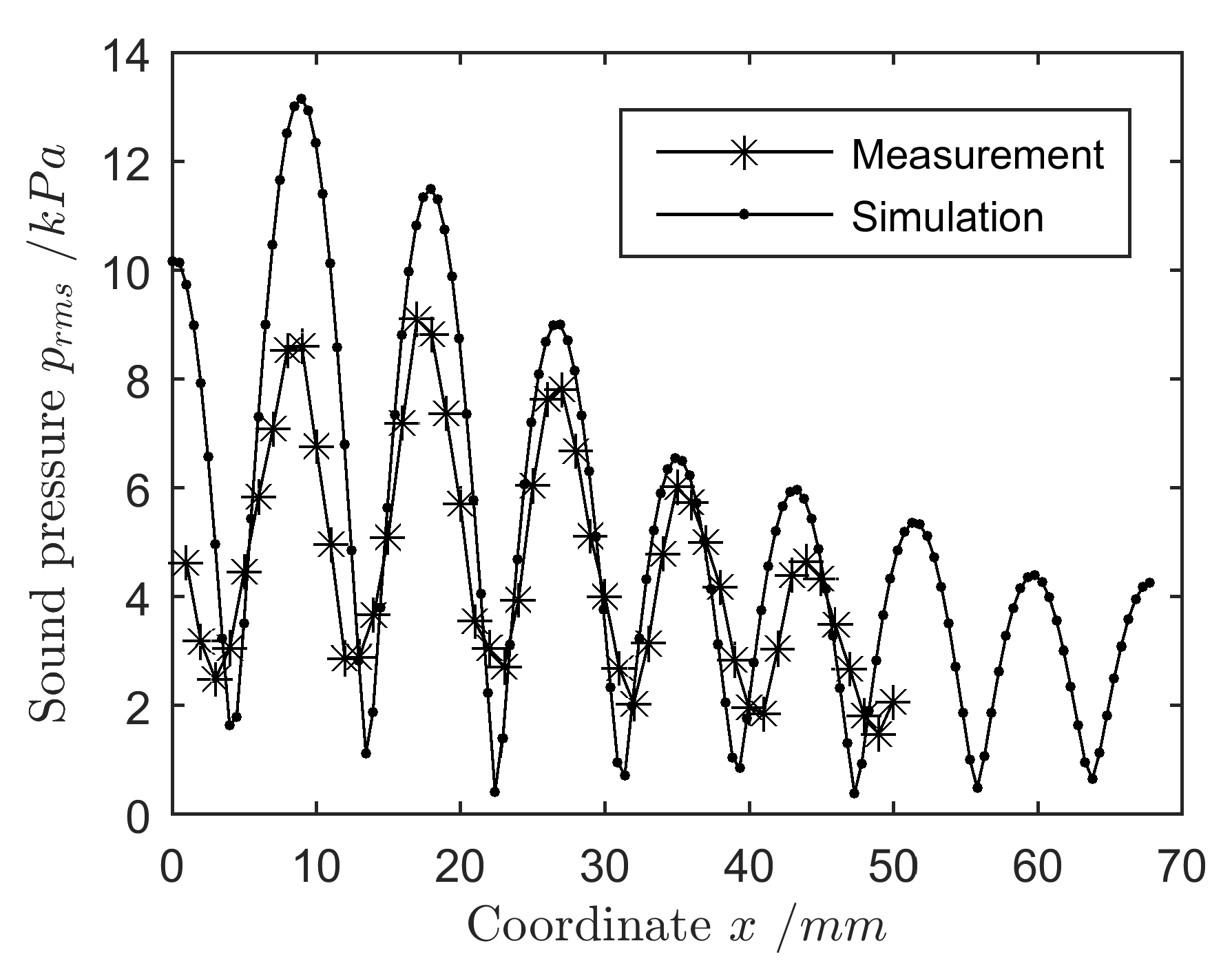
Figure 17 shows a comparison of sound pressures predicted by the model and from experiments for a standing wave system with concave reflector at the optimal distance of $L=4\lambda$. As already expected, the deviations are large in areas of high sound pressure. Since the model does not consider the nonlinearities, the sound pressures in the model are much too high. However, the agreement is good in the areas of lower sound pressure. Furthermore, the sound pressure in the sound pressure nodes of the experiment does not decrease as much as in the model, since in the experiment higher harmonics occur (see Figure 10), which might not be zero in the sound pressure node.

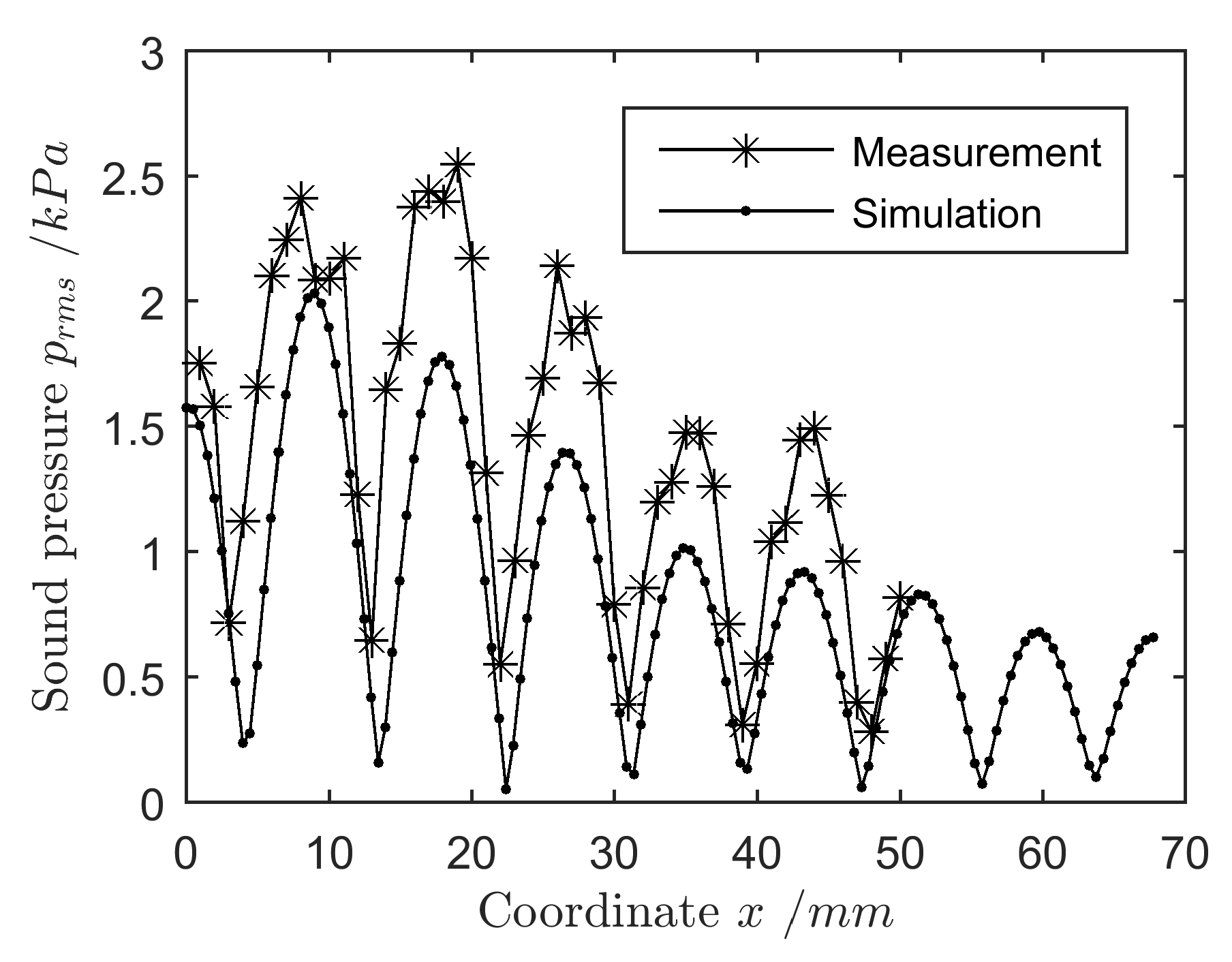
To exclude the nonlinearities in the comparison, measurements and simulations were carried out at smaller excitation amplitudes, too. Figure 18 shows the sound pressures from measurement and simulation at an excitation amplitude of 2 $\mathsf{\mu }$m. The deviations between simulation and measurement are much smaller and are probably only caused by inaccuracies in the measurement of the excitation amplitude and the sound pressure.

6. Conclusions and Outlook

It was shown that the maximum sound pressure level in standing wave systems can be increased by optimizing the geometry and distance of the reflector. A linear finite-element model was used to perform a model based optimization of a standing wave system. The validation with an experimental setup, consisting of a piezoelectric ultrasound transducer and one or more reflectors in different shapes was successful. However, it was found that the nonlinear effects occurring at high sound pressure levels led to higher deviations of the absolute sound pressure level of the model. Nevertheless, the sound field pattern of the model is in very good accordance to experiments. This allows an optimization of the geometric boundary conditions (like shape of reflector and distance) of the sound field.

The highest sound pressure levels can be achieved when the distance between the transducer and the reflector is set to $\lambda /2$, regardless of which reflector is used. For larger distances it is recommended to use a concave reflector, resulting in a second optimum at a distance of about $L\approx R$. According to measurements, an increase of the sound pressure by $400\%$ and more was possible by just using a concave reflector instead of a plain one. When even larger distances are needed, concave reflectors can be used on both sides, enabling high sound pressure levels at a distance between transducer and reflector of about $L\approx 2R$.

The optimization of the standing wave system enabled the atomization of highly viscous liquids with dynamic viscosities greater than 1000 mPas at a throughput of 1 mL/s. The described standing wave system was driven at an electrical power of less than $20W_{rms}$. However, the model and the optimization approach can also be used for systems with larger power output, enabling the dispersion of fluids with even higher viscosity or at higher throughput.