Article

A Novel Solution for the Elimination of Mode Switching in Pump-Controlled Single-Rod Cylinders

Department of Engineer Sciences, University of Agder, 4879 Grimstad, Norway
*
Author to whom correspondence should be addressed.
Actuators 2020, 9(1), 20; https://doi.org/10.3390/act9010020
Submission received: 31 January 2020 / Revised: 8 March 2020 / Accepted: 11 March 2020 / Published: 14 March 2020
(This article belongs to the Special Issue Electro-Hydraulic Actuators)

Abstract

:
This paper concerns the stability issue of pump-controlled single-rod cylinders, known as mode switching. First, a review of the topic is provided. Thereafter, the most recently proposed solution for the elimination of mode switching is investigated and shown to result in unstable behavior under certain operating conditions. A theoretical analysis is provided demonstrating the underlying mechanisms of this behavior. Based on the analysis, a novel control strategy is proposed and investigated numerically. Proper operation and stability are demonstrated for a wide range of operating conditions, including situations under which the most recently proposed solution results in unstable behavior and loss of control over the actuator.

1. Introduction

Pump-control of hydraulic actuators is a promising technology offering several advantages over traditional valve-controlled systems. By connecting a hydraulic pump directly to the actuator, its velocity may be controlled by varying either the speed of the prime mover, the displacement of the pump, or a combination of both [1]. This eliminates the need for throttling of the hydraulic fluid, allowing energy efficiencies superior to that of conventional valve-controlled systems [2,3]. This also facilities the construction of compact electrohydraulic drives, combining the advantages of electrical actuation (e.g., energy efficiency, plug-and-play functionality and no external piping) with those of the hydraulic actuation (e.g., long service life, high force availability and good overload protection) [2,3,4].
A common requirement in industrial applications is the use of single-rod cylinders. This results in different flows into, and out of, the cylinder, which must be handled for proper operation of the actuator. Several solutions exist, involving either, the use of multiple pumps or auxiliary valves [5,6,7,8]. Conceptually, the simplest solution involves a switching valve arrangement that connects one of the cylinder chambers to a hydraulic reservoir, displacing the differential flow to and from the reservoir as the actuator is operated. A simple and cost-efficient circuit enabling four-quadrant operation utilizing a shuttle valve to realize this function was introduced by Hewett [9], followed by a circuit utilizing pilot operated check valves (POCVs) by Rahmfeld and Ivantysynova [10]. In both cases, the differential flow is compensated by monitoring the pressures of the actuator and connecting the cylinder chamber with the lowest pressure to the reservoir, see Figure 1 [11]. These solutions have, however, shown to exhibit unstable behavior. Under certain operating conditions, the switching valve arrangement may oscillate, reversing its connections rapidly, even for a constant input (i.e., constant velocity of the electric motor, or displacement of the pump). This results in oscillations of the pressures and velocity of the actuator, which may lead to reduced performance and loss of control over the actuator [8,9,10]. This phenomenon is commonly referred to as mode switching, first described by Williamson and Ivantysynova [12]. Alternative solutions, using multiple pumps to handle the differential flow, does not result in mode switching [11]; however, a solution utilizing a single pump is more attractive with regards to compactness and system cost. For this reason, much research effort has been devoted to investigating the causes and potential solutions for mode switching in single-pump circuits, a review of which is presented in the following.
Williamson and Ivantysynova first reported mode switching while lowering light loads at high velocity [12], then later for large inertia loads subjected to low external forces [13]. Feedforward control of the actuator pressures, by means of a predictive observer was proposed, however later found to be an insufficient solution [13].
A numerical analysis using a simplified nonlinear model was presented in [13], studying inertia loads from 1 to 20 ton. Approximate stability thresholds were derived based on the study, and mode switching was shown to increase for increasing inertias and lower damping. The use of pressure feedback was proposed, and shown to be capable of stabilizing the actuator for the operating conditions considered. Michel and Weber demonstrated that mode switching may result from subjecting large inertia loads to high accelerations, and derived the limit for the maximum acceleration that may be safely applied [11]. Pressure feedback was reported to be capable of increasing this limit [11]. A mathematical analysis was presented in [14], where it was shown that instability may occur at low load conditions.
The introduction of leakage to dampen mode switching oscillations by means of two auxiliary hydraulic valves was proposed in [14], and shown to prevent mode switching for the operating conditions investigated using a load of 143 kg. A more detailed analysis was presented by Caliskan et al. by also including the dynamics of the switching valve arrangement, which had previously been treated as an ideal switching element. Using linearized analysis, the presence of unstable equilibrium points was demonstrated. The introduction of leakage without auxiliary valves was proposed using an underlapped shuttle valve and shown to provide stable operation up to certain retraction speeds [15,16]. The effects of friction and line losses were studied in [17] and shown to alter the regions of stable and unstable operation. Stabilization of the actuator by means of throttling only during critical operating conditions (i.e., low load conditions) was studied in [17,18], and shown to improve performance while preserving high energy efficiency.
All of the research reviewed so far concerns solution utilizing the valve switching strategy of connecting the lowest cylinder chamber pressure to the reservoir. Although improvements have been made, every proposed solution has suffered from performance issues and instability under some operating conditions [19,20]. These solutions have typically been analyzed based on a quadrant division plotting the velocity of the actuator on the vertical axis versus the external force on the horizontal axis. Recently, Costa and Sepehri analyzed the problem from a different perspective by introducing a new quadrant division. Rather than using the external force, the force due to the hydraulic pressures, referred to here as the hydraulic force F h y d , was used on the horizontal axis [19]:
F h y d = p 1 A 1 p 2 A 2 .
where p 1 and p 2 are the piston- and rod-side pressures, and A 1 and A 2 are the piston- and rod-side areas. It was shown that previous quadrant divisions do not accurately describe the operating quadrants of the cylinder, and this was proposed as an explanation for why previous attempts of solving the problem of mode switching have failed. A new valve switching strategy, based on the direction of the hydraulic force, was proposed and implemented hydraulically by means of a pressure intensifier. Experimental results controlling a load of 367 kg were presented with stable four-quadrant operation demonstrated for the operating conditions investigated [19,20]. This is the most recently proposed control strategy for single-pump circuits and is referred to here as the steady-state switching law (SSL).
This paper concerns the stability and control of simple-pump circuits utilizing switching strategies based on the new quadrant division of Costa and Sepehri. First, the stability of a pump-controlled single-rod cylinder using the SSL is investigated in detail. It is demonstrated theoretically and numerically that mode switching may still occur under some operating conditions using the SSL. A theoretical analysis is provided that explains the underlying mechanisms of this behavior. Based on the analysis, a novel switching strategy is proposed and investigated. A number of operating conditions are presented in which the use of the SSL leads to mode switching in varying degrees, with the most severe cases resulting in loss of control over the actuator. It is demonstrated that neither artificial damping nor filtering of the hydraulic force prevents mode switching using the SSL under these conditions. Operating conditions leading to mode switching are presented for both low and high load conditions, as well as low and high velocities, for a load of 2000 kg. The same simulations are then repeated using the proposed control strategy, with stable behavior free of mode switching demonstrated for all these operating conditions. Finally, stable behavior, free of mode switching, is demonstrated using the proposed strategy for a wide range of external loading.
The rest of the paper is organized as follows: Section 2 describes the system under consideration and its mathematical model. In Section 3, the possibility of mode switching using the SSL is demonstrated and analyzed. A novel control strategy is proposed in Section 4, with numerical results presented in Section 5. Section 6 concludes the paper with a summary of the findings.

2. System under Consideration

2.1. Hydraulic Circuit and Control Algorithm Implementation

The single pump circuit implementation, considered here, is shown in Figure 2. Traditionally, single-pump-control strategies such as the SSL and its predecessor have been implemented using purely hydraulic implementations [2,7]. Here, the use of two electronically actuated ON/OFF valves ( E V 1 and E V 2 ) is proposed for the implementation of the switching law. As will be seen, this enables the application of more sophisticated control algorithms. The novel control strategy of Section 4 requires such an implementation, whereas the SSL may be implemented both hydraulically and electro-hydraulically. In this paper, only electrohydraulic implementations are considered. The results presented here regarding the SSL are however applicable to either implementation. The actuator is controlled by varying the speed of the pump using an electric motor. The results to be presented are, however, equally applicable to variable displacement solutions. Lastly, a sealed accumulator is used as the hydraulic reservoir, so that the resulting system is a self-contained unit.
Referring to Figure 2, the SSL may be implemented electro-hydraulically as follows. The hydraulic force F h y d is defined as in (1). For F h y d > 0 , E V 1 is closed while E V 2 is open. For F h y d < 0 , the valve connections are reversed.

2.2. System Modelling

Applying Newton’s second law to the mass m:
m x ¨ = p 1 A 1 p 2 A 2 b x ˙ F e x t ,
where m is the total mass of the piston and load, b is the viscous friction coefficient and F e x t the external force. From the continuity equation:
p ˙ 1 = β 1 V L 1 + A 1 x ( Q p + Q 1 A 1 x ˙ ) ,
p ˙ 2 = β 2 V L 2 + A 2 ( s x ) ( Q p + Q 2 + A 2 x ˙ ) ,
where β 1 and β 2 are the effective bulk moduli, V L 1 and V L 2 the line volumes and s the maximum stroke of the cylinder. The pump flow Q p and the flows through E V 1 and E V 2 :
Q p = D ω c ( p 1 p 2 ) ,
Q 1 = C d A d u 1 s g n ( p 3 p 1 ) 2 ρ | p 3 p 1 | ,
Q 2 = C d A d u 2 s g n ( p 3 p 2 ) 2 ρ | p 3 p 2 | ,
where ω is the velocity of the electric motor, c the pump leakage coefficient, c d and A d the discharge coefficient and discharge area, u 1 and u 2 the normalized openings of the electrohydraulic valves and ρ the fluid density. Assuming an appropriately sized accumulator, the accumulator chamber pressure p 3 is taken as constant. The dynamics of the electrohydraulic valves are modeled as first-order transfer functions with a time constant τ v . The dynamics of the electric motor is modeled as a first-order system with a time constant τ m .

3. Theoretical Analysis

This section demonstrates the possibility of mode switching in pump-controlled single-rod cylinders when controlled using the SSL. For this purpose, consider the circuit of Figure 2, with x ˙ and F e x t positive (resistant load). Assuming steady-state conditions (constant x ˙ , F e x t and ω ), F h y d > 0, and therefore E V 2 is energized while E V 1 is closed. For the sake of clarity of presentation, friction is omitted for the remainder of the analysis. In steady-state, p 2 = p 3 and the cylinder pressures balance according to:
p 1 A 1 p 2 A 2 = F e x t .
Next, consider an abrupt reversal of the external force. From Equations (1) and (8), a switch of the valves will be required. Under these conditions, for the proper operation free of mode switching, the valves must switch only once. If a second switch occurs, a third switch will also be required by necessity before reaching steady-state, meaning that mode switching will take place with a minimum of three switches. Thus, the occurrence of a second switch may be used to demonstrate the presence of mode switching, which is utilized in the following.
Assuming p 1 > p 3 before the switch, p 1 must decrease to p 3 after the valves switch, whereas p 2 must increase to fulfill Equation (8). During this transition, from the SSL and the definition of the hydraulic force, the valves will switch a second time if p 2 < p 2 , with p 2 defined as:
p 2 = p 1 A 1 A 2 .
This switching condition may be illustrated graphically as in Figure 3, where the pressure p 2 is shown (solid line) along with the switching threshold p 2 (dashed line). The valve switching process may be divided into four distinct stages, numbered one through four in Figure 3.
During the first stage ( t < t 1 ), the system is in steady-state with:
p 2 = p 3 ,
p 2 = p 3 + F e x t A 2 ,
At t = t 1 , the external force changes direction, which marks the onset of the second stage. As a result, p 1 and thus also p 2 will decrease, until p 2 reaches p 2 and the valves switch for the first time. The third stage ( t 2 < t t 3 ) is a transient stage, where both p 2 and p 2 must approach their final steady-state values, given by:
p 2 = p 2 , s s = p 3 A 1 A 2 F e x t A 2 .
p 2 = p 2 , s s = p 3 A 1 A 2 .
During the fourth stage ( t > t 3 ), the system is again in steady-state with p 2 and p 2 as described by Equations (12) and (13). Note that for t > t 1 , F e x t is negative, which is why p 2 , s s > p 2 , s s , as indicated in Figure 3. The transient responses of p 2 and p 2 during the third stage determine whether or not a second switch, and thus mode switching, takes place. If p 2 < p 2 at any point after t = t 2 , a second switch will take place and mode switching will occur with a minimum of three switches. The third switch occurs for p 2 > p 2 , after which several set of switches may occur again if the condition p 2 < p 2 becomes fulfilled before reaching steady-state. Referring to Figure 3, this corresponds to an intersection between the curves of p 2 and p 2 .
Observe from (11) that p 2 , s s > p 3 as A 1 > A 2 , and thus both p 2 and p 2 must increase by necessity after the valves switch the first time at t = t 2 . If the gradient of p 2 is less than p ˙ 2 , and the response is well-damped, the situation will resemble that of Figure 4a. In this case, the curves never intersect for t > t 2 , and mode switching does not occur. However, if the gradient of p 2 is greater than p ˙ 2 , the curves will intersect and mode switching will occur with a minimum of three switches. If the gradient of p 2 remains greater than p ˙ 2 after the third switch, a series of switches may be initiated with the curves overlapping until p ˙ 2 < p ˙ 2 . The situation will then resemble that of Figure 4b, where the curves overlap in the region indicated by the green circle. In this paper, this is referred to as type 1 mode switching.
Even in the absence of type 1 mode switching, the curves may intersect at some point during t 2 < t < t 3 if the response of p 2 is underdamped, or the mass m oscillates (thus causing p 2 to oscillate as well). This type of behavior will be referred to here as type 2 mode switching.
These three possible scenarios are demonstrated numerically in the following using the model developed in the previous section. Starting at steady-state with x = 0.1 m , m = 100 kg , b = 4000 N s / m , ω = 40 rpm , ideal (infinitely fast) valves, and the remainder of the system parameters as presented in Section 5, an abrupt change in F e x t from 1 kN to 1 kN at t = 0.1 s is simulated and plotted in
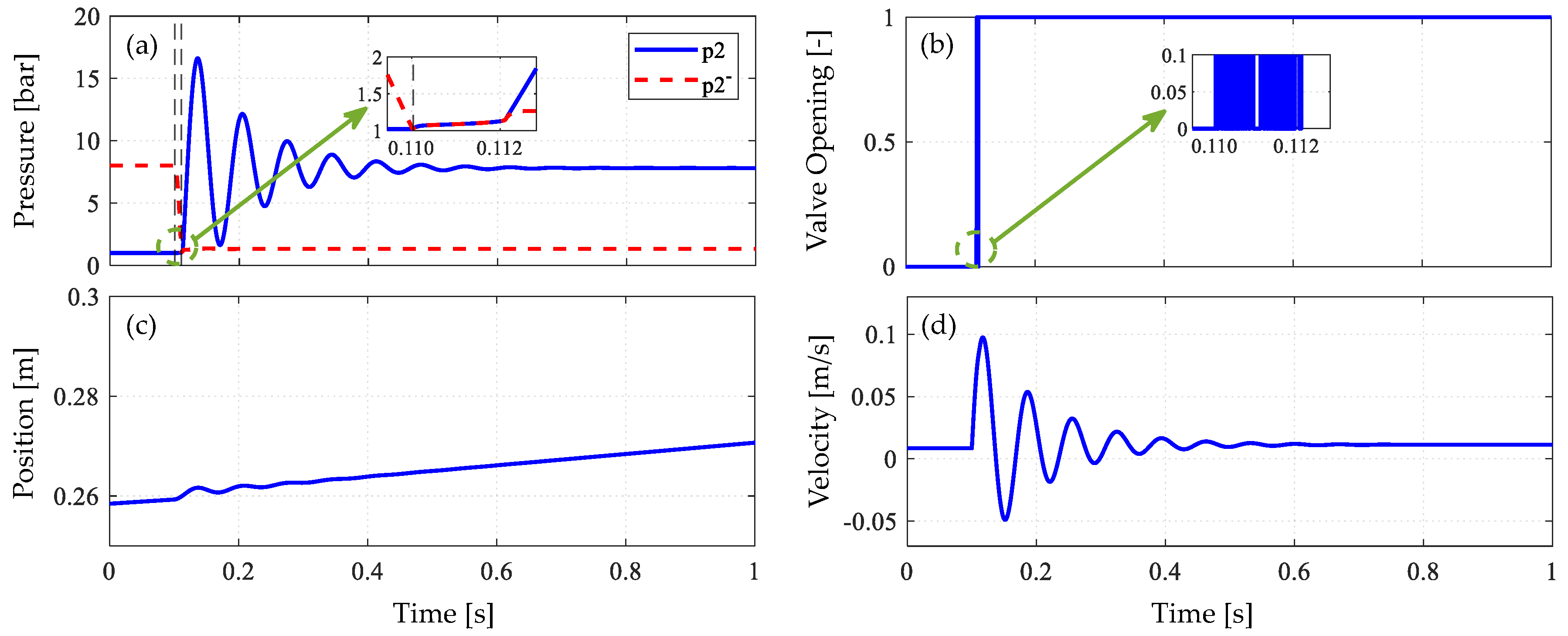
 Figure 5. Figure 5a shows the response of p 2 along with the switching threshold p 2 , and Figure 5b shows the state of the E V 1 valve, where 1 indicates an open valve and 0 indicates the valve being closed. The response of the second valve, E V 2 is identical in shape but reversed. The position and velocity of the actuator are given in Figure 5c,d, respectively. In Figure 5a, the external force changes direction at the time indicated by the first dashed horizontal line, whereas the second dashed horizontal line indicates the time when the valves switch for the first time. As seen in Figure 5a, for these system parameters and operating conditions, p 2 and p 2 never intersect after the valves switch the first time, and thus mode switching does not take place.
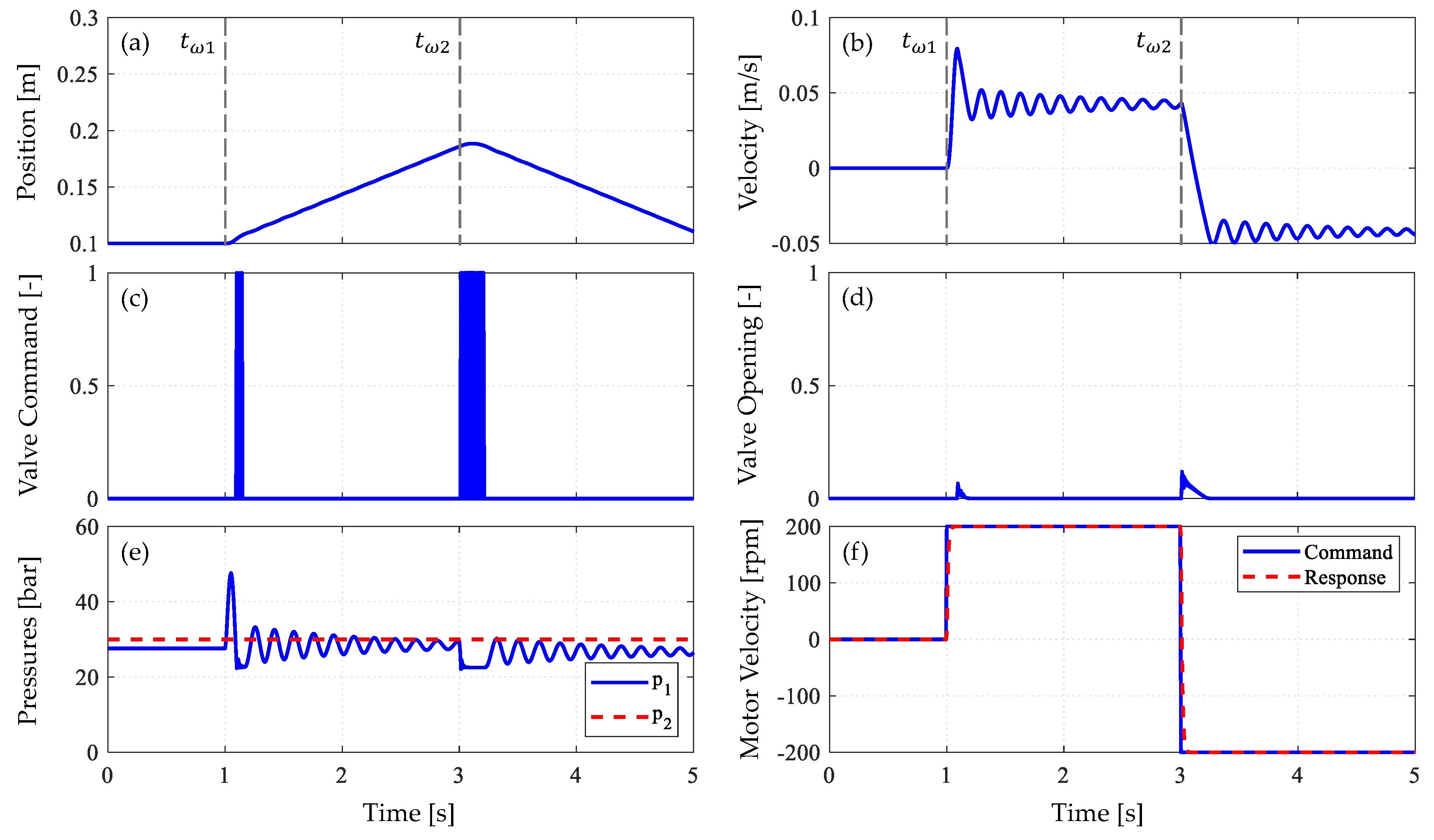
Next, the simulation is repeated with m = 200 kg . As seen in Figure 6a, under these conditions the curves intersect continuously for a short period of time after the valves switch for the first time, leading to a series of switches, as seen in Figure 6b, demonstrating type 1 mode switching. During this short time period, using ideal valves and a simulation step time of τ s i m = 10 6 s , a total of 49 switches take place.
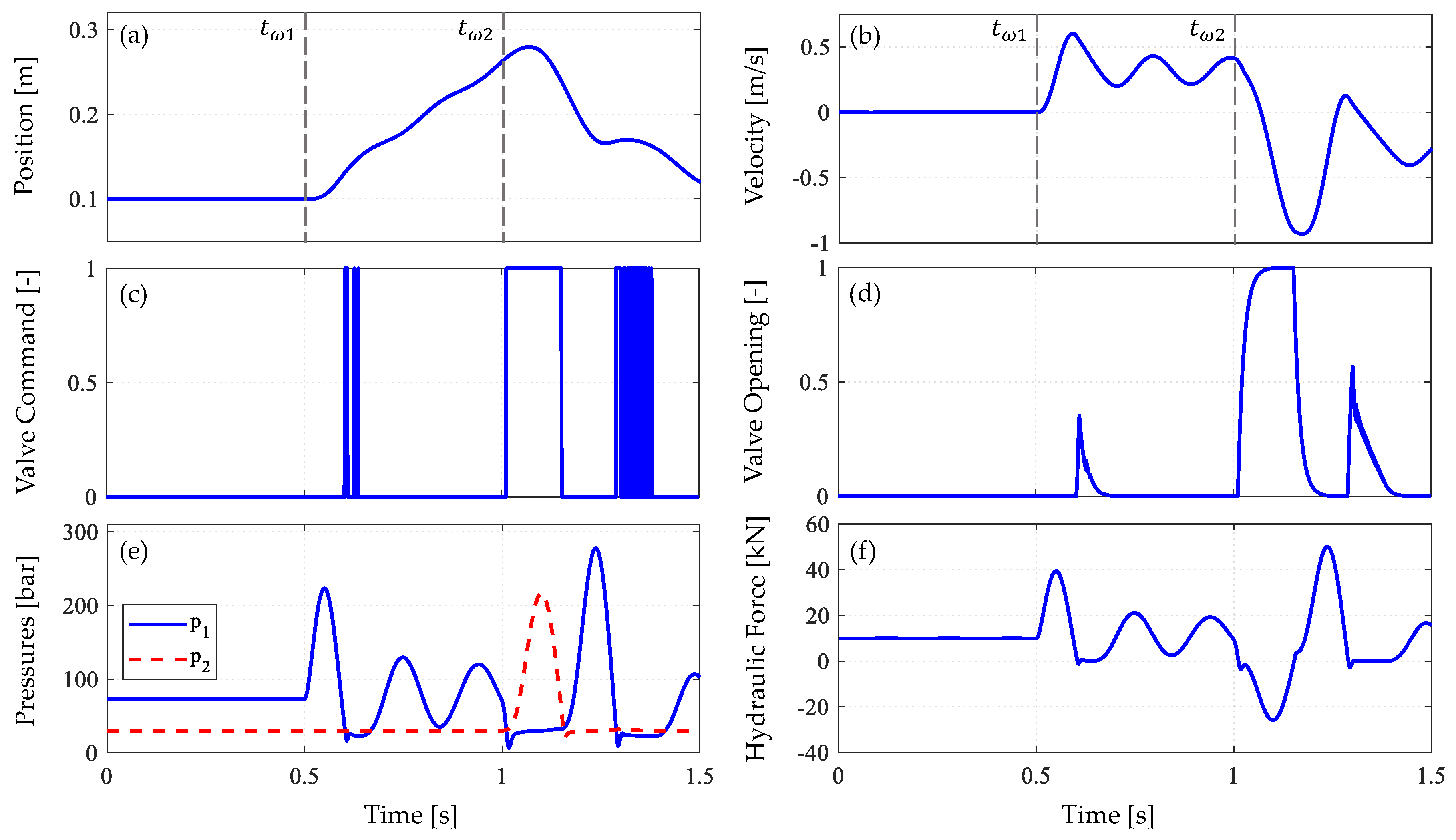
Repeating the simulation with a mass of m = 2000 kg , the results plotted in Figure 7a–d are obtained. Under these conditions type 1 mode switching occurs for a longer period of time after the initial valve switch, followed by a type 2 mode switch at approximately t = 0.4 s . Type 1 and type 2 mode switching then occur consecutively for the remainder of the simulation with a total of 23479 switches taking place. The effect of this mode switching on the position and velocity of the actuator is clear from Figure 7c,d, where both the position and velocity are observed to oscillate. Obviously, this is not an acceptable type of behavior.
The analysis presented here was conducted using an abrupt change in the external force. This represents the worst-case scenario, and may also represent an abrupt acceleration or deceleration of the actuator, which is investigated in Section 5.
The results of the analysis may be summarized as follows:
  • Although, the SSL provides the correct operating quadrant and steady-state behavior, mode switching may occur under certain operating conditions due to dynamic considerations. Additionally, two distinct types of mode switching have been identified, referred to here as type 1 and type 2.
  • The salient feature of type 1 mode switching is a continuous series of high-frequency valve switches, and its occurrence depends upon the gradients of the cylinder pressures. This type of mode switching may thus occur even if the pressures of the system are well damped.
  • If the pressures are not well-damped, any factor causing either cylinder chamber pressure to oscillate (such as oscillations of the mass m ) may result in a series of low-frequency switches, which has been defined here as type 2 mode switching.

4. Novel Control Strategy

4.1. Conceptual Development

Referring to the summary of the previous section: regarding the third point, damping of the pressures or filtering of F h y d is likely to be beneficial. The former may be achieved by introducing leakage or artificial damping (e.g., acceleration or pressure feedback), whereas the latter may be easily implemented in software when using an electrohydraulic valve implementation. Regarding the second point however, neither damping nor filtering are expected to resolve type 1 mode switching, and therefore an alternative solution is developed here. Both artificial damping and filtering of F h y d will, however, be evaluated in Section 5, along with the control strategy to be developed in this section.
From its definition, the hydraulic force is observed to be comprised of the following components, which in turn dictate whether or not a valve switch is commanded at any given time:
F h y d = F e x t + F a , ω + F f + F v s + F a , m ,
which are numbered here as one through five and defined as: (1) F e x t : the external force, (2) F a , ω : forces from commanded accelerations by adjusting the velocity command sent to the electric motor, (3) F f : frictional forces, (4) F v s : forces arising from transient pressure changes as a result of a previous valve switch, (5) F a , m : forces due to oscillations of the mass m .
The analysis presented in the previous section indicates that reacting to the fourth and fifth components is not desirable as it may lead to type 1, and type 2 mode switching, respectively. With this in mind, the modified hydraulic force F m o d is introduced and defined as:
F m o d = F e x t + F a , ω + F f ,
The control strategy proposed here is to continuously calculate an estimate of the modified hydraulic force, denoted F ^ m , by means of an observer, and command valve switches based on F ^ m o d rather than F h y d . This should eliminate mode switching, however as a result the system may experience transiently a valve connection which is considered incorrect according to the SSL and its predecessor, in particular near F h y d = 0 . The effects of having such a connection, referred to here as a reverse connection, is therefore investigated in the following before concluding the development of the proposed strategy.
Referring to Figure 2, assuming steady-state conditions and F e x t positive, E V 2 should be energized with E V 1 deenergized according to the SSL. Reversing the connections, p 1 = p 3 while p 2 is given by Equation (8) as:
p 2 = p 3 A 1 A 2 F e x t
From Equation (16) it is seen that as long as the following condition is fulfilled:
p 3 A 1 A 2 F e x t > 0 ,
having a reverse connection will not lead to cavitation and thus control over the actuator is retained. From Equation (17) it is seen that by increasing the accumulator pressure p 3 , the system remains controllable with a reverse connection for larger F e x t . For the system under consideration with parameters as given in Section 5 and an accumulator pressure of p 3 = 1 bar , it is found by rearranging Equation (16) that the system can tolerate a reverse connection for up to F e x t = 196 N for positive F e x t ( E V 1 energized), and down to F e x t = 147 N for negative F e x t ( E V 2 energized). Increasing the accumulator pressure to p 3 = 30 bar , these limits increase to F e x t = 5890 N , and F e x t = 4418 N , respectively. The same deduction applies to F h y d for transient behavior.
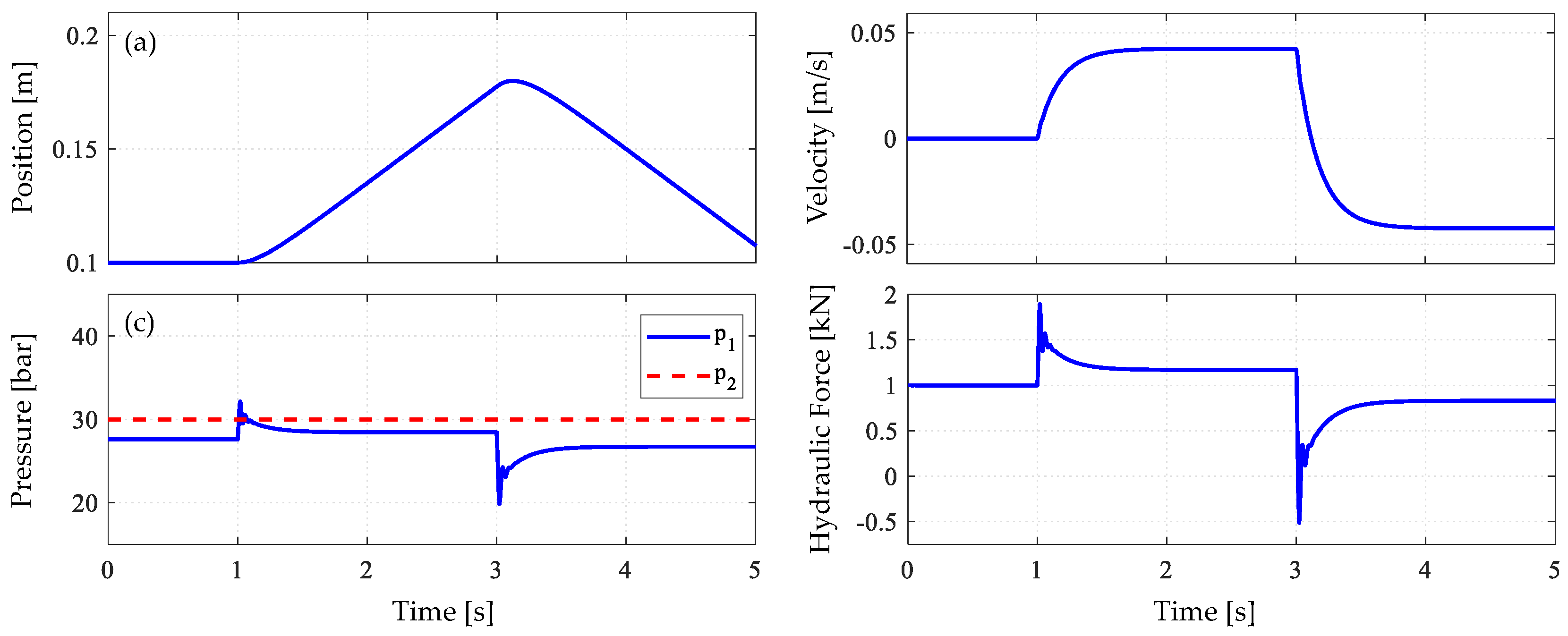
This is verified numerically in Figure 8, where the system is simulated with ω = 0 rpm for t < 1 s , ω = 400 rpm , ω = 400 rpm for t > 3 s , p 3 = 30 bar and an external force F e x t = 1 kN . Figure 8a–c show the position, velocity and pressures of the system with constant valve openings u 1 = 1 and u 2 = 0 for the entire duration of the simulation. Figure 8d shows the hydraulic force, which is seen to be positive except for a short period of time during t = 3 s .
Under these conditions, the system maintains a reverse connection for the entire simulation except for the short time period where F h y d becomes negative. Despite the reverse connection, the system does not cavitate and remains both controllable and well behaved. The same simulation is repeated in Figure 9, however with u 1 = 0 and u 2 = 1 , providing the system with a reverse connection only transiently near t = 3 s . Although the position and velocity response of the actuator differ slightly from that of Figure 8, the system remains controllable, well behaved and free of cavitation.
Continuing with the development, the proposed strategy involves ensuring a certain minimum pressure of the hydraulic reservoir, taken here as p 3 = 30 bar , which may be realized using an appropriately sized hydraulic accumulator as the reservoir. For a compact cylinder drive, this is not common practice, where typically much lower accumulator pressures are used (e.g., p 3 = 1 bar ) [21]. As a result, some changes in the hydraulic topology are required. For variable-displacement drives however, the use of a low-pressure line with a pressure of e.g., p 3 = 25 bar is already common practice in order to supply the servo valve controlling the displacement of the hydraulic unit from the same line. Increasing the accumulator pressure also improves the stiffness of the actuator, leading to more favorable dynamics. However, the force capability of the actuator is also reduced, and thus, selecting the accumulator pressure level constitutes a tradeoff [22].
Although maintaining a constant set of valve opening leads to an appropriate behavior free of mode switching under these conditions, as soon as F h y d goes outside the limits calculated from Equation (16) with F h y d inserted for F e x t , the system will cavitate and a switch of the valves is required to maintain control over the actuator. Switching the valves at points close to these limits is not a feasible control strategy as this would introduce large pressure shocks into the system. Switching of the valves should therefore, take place near close to p 1 = p 2 (e.g., F h y d = 0 ). The proposed control strategy may then be summarized as follows: (1) Implement the system with an appropriate pressure p 3 . (2) Estimate the modified hydraulic force F m o d using an observer. (3). For F m o d > 0 N , energize E V 2 , for F m o d < 0 N , energize E V 1 .

4.2. Implementation

The implementation of the proposed strategy is realized as follows:
  • An observer is constructed using equations identical to those presented in Section 2, except that the switching valves E V 1 and E V 2 are excluded from the model in the observer and the pump is modelled as an asymmetrical pump whose input and output flows are scaled to match the differential area of the cylinder. This system, referred here as the virtual system is then simulated in parallel with the true process. Additionally, the external force F e x t is estimated using a simple proportional Luenberger observer with a gain of K o b s v , F , implemented as described in [23].
  • The pressures of the virtual system, p 1 v i r t and p 2 v i r t are used to estimate of the modified hydraulic force as F ^ m = p 1 v i r t A 1 p 2 v i r t A 2 .
In this manner, the fourth component (transient pressure behavior due to valve switches) of Equation (14) no longer affects the switching of the valves. The effects of the fifth component (mass oscillations) are then eliminated by introducing a strong acceleration feedback with a feedback gain K a , v i r t in the virtual system.
Additionally, in order to ensure that the virtual system closely follows the desired velocity of the true system, a velocity feedback with a feedback gain of K v , v i r t is introduced in the virtual system. The set point of this velocity feedback is calculated by estimating the desired velocity of the true system based on a filtered version of the velocity command sent to the electric motor, u m , f i l t , as:
x ˙ v i r t , r e f = D u m , f i l t ( A 1 + A 2 ) / 2
where x ˙ v i r t , r e f is the velocity reference, and the average values of the cylinder areas have been used as the velocity gain of the true system is a function of A 1 with E V 2 is energized, while a function of A 2 when E V 1 is energized. For filtering of the velocity command, a first-order filter with a time constant of τ r e f , v i r t is utilized. Lastly, in order to prevent valve switches from minor fluctuations in F ^ m o d when F ^ m o d remains close to zero, a fixed valve configuration ( E V 1 = 1 and E V 2 = 0) is maintained whenever F ^ m o d enters a certain threshold value | F ^ m o d | = y 1 , which is deactivated again when | F ^ m o d | = y 2 . To avoid oscillation between these two modes of operation, referred to here as fixed behavior, and virtual behavior, respectively, y 2 is selected as y 2 > y 1 .
An overview of the virtual system is shown in Figure 10, where G v i r t is the mathematical model of the valveless system containing the asymmetrical pump. The pressures of G v i r t are then used to estimate the hydraulic force to control the valves of the true system. Although the virtual system contains both a velocity and an acceleration feedback, the true system may be controlled in an open-loop manner from input to output velocity, with or without acceleration feedback.
These parameters (i.e., K o s b v , F , K a , v i r t , K v , v i r t , τ r e f , v i r t , y 1 and y 2 ) may then be tuned and optimized until the desired system behavior is achieved. With the proposed control strategy, referred to here as the virtual system switching law (VSL), the desired system behavior is for the valves to switch based on the factors contained in the modified hydraulic force of Equation (15), i.e., the external force, force components, due to commanded accelerations and frictional forces. Regarding frictional forces, only viscous friction is considered here. Note that although, the virtual system uses both velocity and acceleration feedback, the true system may be controlled in either open-loop or in a closed-loop manner.

5. Numerical Results

This section presents numerical results using the SSL and VSL control algorithms.

5.1. Model Parameters and Operating Conditions

The models presented in Section 2 and Section 4 are implemented in MATLAB using forward Euler integration with a time step of τ s i m = 10 6 s and system parameters as given by Table 1. For simulations with low velocity, the system starts at rest in steady-state with x = 0.1 m , x ˙ = 0 m / s and ω = 0 rpm , followed by an abrupt acceleration at t = t ω 1 = 1 s by commanding the electric motor to ω = 200 rpm , and a command to reverse with ω = 200 rpm at t = t ω 2 = 3 s . For simulations with higher velocities, the operating conditions are similar, however with the electrical motor commanded to ω = 1500 rpm ( t = t ω 1 = 0.5 s ) and ω = 1500 rpm ( t = t ω 2 = 1 s ).

5.2. Steady-State Switching Law (SSL)

First, the system is simulated under low load conditions ( | F e x t | 1 kN ) at low pump velocities ( | ω | 200 rpm ) with the valves controlled using the SSL. Figure 11 shows the position, velocity, valve command ( E V 1 ), valve opening ( E V 1 ) and pressures of the actuator for a constant external force of F e x t = 1 kN . Based on the operating conditions, a transient switch of the valves is required at t = t ω 2 in order to accommodate for the abrupt reversal of the actuator. Aside from this, no other switches are required considering the external force, acceleration and viscous friction. Observe from Figure 11c, however, that the valves also switch at t = 1 s . Furthermore, a series of multiple high-frequency switches occur at both t = 1 s and t = 3 s . This is a result of mode switching, as the control law also responds to other factors such as valve transients and mechanical oscillations. The position and velocity responses of the actuator are however acceptable, and control over the actuator is maintained.
The simulations are then repeated with F e x t = 0.1 kN , with the results plotted in Figure 12. Under these conditions, the system enters a continuous state of mode switching after the pump is reversed at t = tω2. From Figure 11a,b, this is seen to result in reduced performance, with the actuator moving at a much lower velocity than previously for t > t ω 2 .
Next, a variable external force is introduced with F e x t = 0.1 kN up to t = t F = 2 s and F e x t = 0.1 kN for t t F . As seen in Figure 13a,b, this results in loss of control over the actuator, with the actuator extending positively for the entire despite commanding a reversal at t = t ω 2 This is clearly an unacceptable response.
In an attempt to improve the behavior of the system, filtering of F h y d is introduced using a first-order filter with a time constant of 150 ms . The results are given in Figure 14 with Figure 14f displaying the original F h y d along with its filtered value. Despite heavy filtering, control over the actuator is still lost as a result of the mode switching. Even with a time constant of 1500 ms , the authors were unable to achieve a stable response.
As an alternative remedy, artificial damping is evaluated by introducing an acceleration feedback with a gain of K a = 80 s / m 2 , which increases damping in the same manner as leakages, however without resulting in energy losses. As seen in Figure 15b,e, the damping of the system has increased substantially as a result of the acceleration feedback. Despite the increased damping, however, the system still experiences continuous mode switching for t > t ω 2 , resulting in loss of control over the actuator.
Figure 16 demonstrates similar behavior under acceleration feedback for a variable external force of magnitude | F e x t | = 1 kN . Note in Figure 16a that as a result of having lost control, the actuator reaches end its end stop close to t = 4 s and the simulation is therefore concluded.
Lastly, operating conditions where the use of the SSL results in degraded performance are presented for higher velocity commands of the actuator. Figure 17 and Figure 18 illustrates the response of the actuator for a commanded pump velocity of | ω | = 1500 rpm under both low ( F e x t = 1 kN ) and high load conditions ( F e x t = 10 kN ) without the use of filtering or acceleration feedback. In both situations, mode switching occurs and results in significant loss of performance of the actuator. Thus it is demonstrated that the use of the SSL may result in mode switching for both low and high actuator velocities, and also under both low and high loading conditions.

5.3. Virtual System Switching Law (VSL)

Next, the system is simulated under the same operating conditions with the valves controlled according to the VSL. The tunable parameters of the VSL are selected as shown in Table 2. Additionally, the system is provided with an acceleration feedback with a gain of K a = 40 s / m 2 .
Starting with a constant external force of F e x t = 1 kN and a commanded pump velocity of | ω | = 200 rpm , the response of the system is given in Figure 19 (VSL) for the same operating conditions as those of Figure 11 (SSL). Based on the external force and commanded acceleration, the desired behavior of the valves is a transient switch shortly after t = t ω 2 in order to accommodate for the reversal of the actuator. As seen in Figure 19c,d, this exact behavior is achieved using the VSL, with only a transient reversal of the valve connections occurring shortly after t = t ω 2 as the actuator reverses direction. Compare with Figure 11 (SSL). Aside from this, no other valve switches occur and mode switching is avoided. A minor disturbance in the velocity of the actuator is observed in Figure 19b as the valves reverse, the response of the actuator is however well behaved and acceptable. Figure 19f shows the estimate of the modified hydraulic force used in the VSL, along with the original hydraulic force used for the SSL.
Figure 20 shows the response of the system for a constant external force of F e x t = 0.1 kN . Recall from Section 4, that with the VSL a fixed valve configuration is maintained for | F ^ m | y 2 after | F ^ m | = y 1 , which is referred to as fixed behavior. In Figure 20, F ^ m remains inside this threshold and the system is, therefore, operating in the fixed behavior mode with no valve switches occurring. The overall response of the actuator is both well behaved and acceptable. Compare with the degraded performance resulting from the use of the SSL in Figure 12a,c for the same operating conditions.
Next, the variable external force of Figure 13, Figure 14 and Figure 15 (SSL) is introduced using the VSL, the results of which are plotted in Figure 21. As with the previous simulation, the system is operating in fixed behavior mode and as a result no valve switches occur. The response of the system is both acceptable and well behaved. Compared to Figure 13, Figure 14 and Figure 15 (SSL), where control over the actuator was lost using the SSL for the same operating conditions for t > t ω 2 . Using the VSL, however, control over the actuator is maintained throughout the entire simulation, with the actuator successfully following the command to reverse direction.
Increasing the magnitude of the variable external force to | F e x t | = 1 kN , the system now operates in the virtual behavior mode (i.e., valve switches are commanded based on the direction of F ^ m ), see Figure 22. Under these conditions, only a single switch of the valves is expected at t = t F as the external force changes direction. No additional switches are required to accommodate for the reversal of the actuator at t = t ω 2 as the external force is negative for t t F . As seen in Figure 22, this exact behavior is achieved using the VSL, with the valves switch only once. Due to a large change in the external force, a significant velocity disturbance is introduced at t = t F , the response of the actuator is, however, both acceptable and well behaved. Compared to Figure 16 (SSL) where control over the actuator is lost under the same operating conditions, the external force along with its estimated value is shown in Figure 22f, which is observed adequately despite minor drifting.
Figure 23 illustrates the response of the system for a variable force with a magnitude of | F e x t | = 10 kN . Despite an abrupt change in the magnitude of the external of 20 kN at t = t f , the response remains stable and control over the actuator is maintained. Aside from the effects of the shock introduced by reversing an external force of this magnitude at t = t f , the response of the system remains acceptable and well behaved. The estimate of the modified hydraulic force is given in Figure 23f along with the hydraulic force used in the SSL, which is seen to behave in a calmer manner around t = t f . This is because the hydraulic force reacts to mechanical oscillations of the combined mass of the piston and the load resulting from the reversal of the external force, whereas the modified hydraulic force reacts only to the commanded motion, viscous friction and the external force itself.
The system is then simulated using the VSL for a wide range of values of the external force, with the external force variable and the commanded motion as in the preceding simulations. The results are given by Table 3, where the behavioral mode of the system is reported along with the number of valve switches and the minimum pressure occurring in either of the cylinder chambers, denoted p m i n . The column denoted controllability indicates whether or not control over the actuator is maintained throughout the simulation.
From the table it is seen that controllability is maintained and cavitation avoided for all operating points, as p m i n > 0   bar . Mode switching is also avoided with only a single switch of the valves taking place. The results thus demonstrate proper behavior of the system when controlled using the VSL for a wide range of operating conditions.
Next, higher speed and loading conditions are evaluated using the same velocity command as in Figure 17 ( | ω | = 1500 rpm ). The response of the system for a constant external force of F e x t = 1 kN and F e x t = 10 kN is given by Figure 24 and Figure 25, respectively. Compare to Figure 17 and Figure 18 (SSL).
In Figure 24, only a single switch of the valves takes place ( t = t ω 2 ), without the valves switching back after reversal of the actuator. This is because of the increased velocity of the actuator, causing the viscous friction to become greater in magnitude than the external force (which is why both F ^ m and F h y d are negative in Figure 24f). In Figure 25, however, the external force is much larger and is not overcome by viscous friction and the valves therefore switch back after having switched transiently to accommodate for the reversal of the actuator. In both cases, the response of the system is well behaved.
In this section it has been demonstrated that, in using the proposed VSL, the system behaves in the intended manner, with valve switches occurring only due to the factors for which the algorithm was designed to execute switches. In this case, the control algorithm was designed to execute switches based on the external force, commanded acceleration and viscous friction, excluding switches due to pressure transients arising from previous switches and mechanical oscillations. The concepts presented here, however, may be used to model any type of switching behavior deemed desirable for a given system configuration. The proposed implementation provides a high degree of flexibility as the algorithm may be easily adjusted in software if performance issues were to arise for a given application. In contrast, previous works have focused primarily on hydraulic implementations, where the control algorithm may not be easily adjusted after the system has been constructed.

6. Conclusions

The results of the paper may be summarized as follows:
  • Mode switching using the steady-state switching law (SSL) recently proposed by Costa and Sepehri has been investigated.
  • It was shown that, as with its predecessor (switching based on p 1 = p 2 ), mode switching may occur under certain operating conditions, resulting in degraded performance or loss of control over the actuator.
  • A theoretical analysis was conducted and two underlying mechanisms were identified for this type of behavior, each leading to a distinct type of mode switching. For this reason, the classification of type 1 and type 2 mode switching was introduced.
  • It was shown that, although the SSL results in the correct operating quadrant and proper behavior steady-state, both type 1 and type 2 mode switching may occur due to dynamic considerations. Using the SSL, type 1 mode switching could not be eliminated by filtering of the hydraulic force nor by the introduction of artificial damping.
  • A novel control strategy consisting of a more sophisticated algorithm, based on the new quadrant division recently introduced by Costa and Sepehri, was proposed and investigated.
  • Numerical results demonstrated proper behavior, and the absence of both type 1 and type 2 mode switching, using the proposed strategy for a wide range of operating conditions, including situations under which use of the SSL, leads to improper operation and loss of control over the actuator.
To the best of the authors’ knowledge, this is the first paper reporting mode switching using the SSL. Experimental validations are therefore called for. An experimental system suitable for this purpose is currently being constructed. Unlike previous works on mode switching, the results presented here are based on the novel quadrant division of Costa and Sepehri. The validity of this quadrant division is neither questioned nor disputed here. In fact, as with the SSL, the proposed strategy is based on this quadrant division.
It has, however, been shown that improper operation may result even with strategies based on this new quadrant division, and further investigations of such phenomena, are therefore, warranted. As with the early works on mode switching using the previous quadrant division, the analysis presented here involves certain simplifying assumptions (e.g., the absence of nonlinear friction, line losses and varying bulk moduli). This has been done with a view of first studying the problem at its core to establish a fundamental understanding. Future works should include investigations of how breaking these assumptions affects performance and regions of stable operation.
The strategy, presented here, has so far shown great promise for the elimination of mode switching, and could possibly be a final decisive solution, or provide the motivation for a new research direction within the field of mode switching in pump-controlled single-rod cylinders, focusing on sophisticated control algorithms implemented in software.

Author Contributions

Conceptualization, P.H.G. and D.P.; methodology, P.H.G., D.P. and M.R.H.; software, P.H.G.; validation, P.H.G., D.P. and M.R.H.; formal analysis, P.H.G..; investigation, P.H.G. and D.P.; writing—original draft preparation, P.H.G.; writing—review and editing, P.H.G., D.P. and M.R.H.; visualization, P.H.G.; supervision, D.P. and M.R.H. All authors have read and agreed to the published version of the manuscript.

Funding

This research received no external funding.

Conflicts of Interest

The authors declare no conflict of interest.

Nomenclature

Abbreviations
E V i Electrohydraulic valves
SSLSteady-state switching law
VSLVirtual system switching law
Symbols
A 1 Piston-side area
A 2 Rod-side area
A d Discharge area
b Viscous friction coefficient
c Pump leakage coefficient
C d Discharge area
F e x t External force
F h y d Hydraulic force
F m o d Modified hydraulic force
K a Acceleration feedback gain
K a , v i r t Acceleration feedback gain, virtual system
K o b s v , F Feedback gain, external force observer
K v , v i r t Velocity feedback gain, virtual system
m Total mass of piston and load
p 1 Piston-side pressure
p 2 Rod-side pressure
p 2 Switching threshold
p 3 Accumulator pressure
p m i n Minimum pressure of the cylinder chambers
p 1 v i r t Piston-side pressure, virtual system
p 2 v i r t Rod-side pressure, virtual system
Q p Pump flow
Q 1 Flow through E V 1
Q 2 Flow through E V 2
s Maximum cylinder stroke
u 1 E V 1 valve command
u 2 E V 2 valve command
u m , f i l t Motor velocity command, filtered
V L 1 Piston-side line volume
V L 2 Rod-side line volume
x Cylinder position
x ˙ Cylinder velocity
x ˙ v i r t , r e f Velocity reference of the virtual system
y 1 Threshold limit, virtual control algorithm
y 2 Threshold limit, virtual control algorithm
β 1 Piston-side bulk modulus.
β 2 Rod-side bulk modulus.
ω Rotational velocity of the electric motor.
τ m Time constant of the electril motor
τ r e f , v i r t Filter time constant, velocity reference of the virtual system
τ v Time constant of the electrohydraulic valves

References

  1. Lovrec, D.; Tic, V.; Tasner, T. Simulation-aided determination of an efficiency field as a basis for maximum efficiency-controller design. Int. J. Simul. Model. 2015, 14, 669–682. [Google Scholar] [CrossRef]
  2. Michel, S.; Weber, J. Energy-efficient Electrohydraulic Compact Drives for Low Power Applications. Fluid Power Motion Control FPMC 2012, 2012, 93–107. [Google Scholar]
  3. Hagen, D.; Padovani, D.; Choux, M. A Comparison Study of a Novel Self-Contained Electro-Hydraulic Cylinder versus a Conventional Valve-Controlled Actuator—Part 1: Motion Control. Actuators 2019, 8, 79. [Google Scholar] [CrossRef] [Green Version]
  4. Padovani, D.; Ketelsen, S.; Hagen, D.; Schmidt, L. A Self-Contained Electro-Hydraulic Cylinder with Passive Load-Holding Capability. Energies 2019, 12, 292. [Google Scholar] [CrossRef] [Green Version]
  5. Ketelsen, S.; Padovani, D.; Andersen, T.; Ebbesen, M.; Schmidt, L. Classification and Review of Pump-Controlled Differential Cylinder Drives. Energies 2019, 12, 1293. [Google Scholar] [CrossRef] [Green Version]
  6. Bonato, C.; Minav, T.A.; Pietola, M.; Sainio, P. Position Control of Direct Driven Hydraulic Drive. In Proceedings of the 8th FPNI Ph.D Symposium on Fluid Power, Lappeenranta, Finland, 11–13 June 2014. [Google Scholar]
  7. Pedersen, H.C.; Schmidt, L.; Andersen, T.O.; Brask, M.H. Investigation of New Servo Drive Concept Utilizing Two Fixed Displacement Units. JFPS Int. J. Fluid Power Syst. 2014, 8, 1–9. [Google Scholar] [CrossRef] [Green Version]
  8. Schmidt, L.; Ketelsen, S.; Brask, M.H.; Mortensen, K.A. A class of energy efficient self-contained electro-hydraulic drives with self-locking capability. Energies 2019, 12, 1866. [Google Scholar] [CrossRef] [Green Version]
  9. Hewett, A.J. Hydraulic Circuit Flow Control. U.S. Patent 5,329,767, 19 July 1994. [Google Scholar]
  10. Rahmfeld, R.; Ivantysynova, M. Energy Saving hydraulic actuators for mobile machines. In Proceedings of the Bratislavian Fluid Power Conference, Casta-Pila, Slovakia, 2–3 June 1998. [Google Scholar]
  11. Michel, S.; Weber, J. Electrohydraulic Compact-drives for Low Power Applications considering Energy-efficiency and High Inertial Loads. In Proceedings of the 7th FPNI PhD Symposium on Fluid Power, Reggio Emilia, Italy, 27–30 June 2012; pp. 1–18. [Google Scholar]
  12. Williamson, C.; Ivantysynova, M. Pump Mode Prediction for Four-Quadrant Velocity Control of Valveless Hydraulic Actuators. In Proceedings of the JFPS International Symposium on Fluid Power, Toyama, Japan, 15–18 September 2008; pp. 323–328. [Google Scholar]
  13. Williamson, C.; Ivantysynova, M. Stability and Motion Control of Inertial Loads with Displacement Controlled Hydraulic Actuators. In Proceedings of the 6th FPNI—PhD Symposium, West Lafayette, IN, USA, 15–19 June 2010; pp. 499–514. [Google Scholar]
  14. Wang, L.; Book, W.J.; Huggins, J.D. A Hydraulic Circuit for Single Rod Cylinders. J. Dyn. Syst. Meas. Control 2012, 134, 011019. [Google Scholar] [CrossRef] [Green Version]
  15. Çalışkan, H. Development and Control of a Single Rod Electro Hydrostatic Actuator. Ph.D. Thesis, Middle East Technical University, Ankara, Turkey, 2015. [Google Scholar]
  16. Çalışkan, H.; Balkan, T.; Platin, B.E. A Complete Analysis for Pump Controlled Single Rod Actuators. In Proceedings of the 10th International Fluid Power Conference, Dresden, German, 8–10 March 2016; pp. 119–132. [Google Scholar]
  17. Imam, A.; Rafiq, M.; Jalayeri, E.; Sepehri, N. Design, implementation and evaluation of a pump-controlled circuit for single rod actuators. Actuators 2017, 6, 10. [Google Scholar] [CrossRef] [Green Version]
  18. Imam, A.; Rafiq, M.; Jalayeri, E.; Sepehri, N. A pump-controlled circuit for single-rod cylinders that incorporates limited throttling compensating valves. Actuators 2018, 7, 2. [Google Scholar]
  19. Costa, G.K.; Sepehri, N. Four-quadrant analysis and system design for single-rod hydrostatic actuators. J. Dyn. Syst. Meas. Control. Trans. ASME 2019, 141, 1–15. [Google Scholar] [CrossRef]
  20. Costa, G.K.; Sepehri, N. A Critical Analysis of Valve-Compensated Hydrostatic Actuators: Qualitative Investigation. Actuators 2019, 8, 59. [Google Scholar] [CrossRef] [Green Version]
  21. Gøytil, P.; Padovani, D.; Hansen, M.R. On The Energy Efficiency of Dual Prime Mover Pump-Controlled Hydraulic Cylinders. In Proceedings of the Fluid Power and Motion Control—FPMC 2019, Longboat Key, FL, USA, 7–9 October 2019. [Google Scholar]
  22. Gøytil, P.H.; Padovani, D. Motion Control of Large Inertia Loads Using Electrohydrostatic Actuation. In Proceedings of the IEEE 16th International Workshop on Advanced Motion Control, Yokohama, Japan, 20 March 2020. [Google Scholar]
  23. George, E. Observers in Control Systems: A Practical Guide; Elsevier: Amsterdam, The Netherlands, 2002. [Google Scholar]
Figure 1. Conceptual schematic of a pump-controlled single-rod cylinder.
Actuators 09 00020 g001
Figure 2. Single-pump circuit under consideration.
Actuators 09 00020 g002
Figure 3. Graphical interpretation of the switching condition.
Actuators 09 00020 g003
Figure 4. Graphical interpretation of the switching condition: (a) no mode switching; (b) type 1 mode switching.
Actuators 09 00020 g004
Figure 5. System response with m = 100 kg , no mode switching: (a) pressure; (b) valve opening; (c) position; (d) velocity.
Actuators 09 00020 g005
Figure 6. System response with m = 200 kg , type 1 mode switching: (a) pressures; (b) valve opening; (c) position; (d) velocity.
Actuators 09 00020 g006
Figure 7. System response with m = 2000 kg , type 1 and type 2 mode switching: (a) pressures; (b) valve opening; (c) position; (d) velocity.
Actuators 09 00020 g007
Figure 8. Constant valve configuration ( E V 1 energized): (a) position; (b) velocity; (c) pressures; (d) hydraulic force.
Actuators 09 00020 g008
Figure 9. Constant valve configuration ( E V 2 energized): (a) position; (b) velocity; (c) pressures; (d) hydraulic force.
Actuators 09 00020 g009
Figure 10. Block diagram overview of the virtual system.
Actuators 09 00020 g010
Figure 11. System response with constant external force, F e x t = 1 kN (SSL): (a) position; (b) velocity; (c) valve command; (d) valve opening; (e) pressures; (f) motor velocity.
Actuators 09 00020 g011
Figure 12. System response with constant external force, F e x t = 0.1 kN (SSL): (a) position; (b) velocity; (c) valve command; (d) valve opening; (e) pressures; (f) motor velocity.
Actuators 09 00020 g012
Figure 13. System response with variable external force, | F e x t | = 0.1 kN (SSL): (a) position; (b) velocity; (c) valve command; (d) valve opening; (e) pressures; (f) motor velocity.
Actuators 09 00020 g013
Figure 14. System response with variable external force, filtering of F h y d (SSL): (a) position; (b) velocity; (c) valve command; (d) valve opening; (e) pressures; (f) force.
Actuators 09 00020 g014
Figure 15. System response with variable external force, acceleration feedback (SSL): (a) position; (b) velocity; (c) valve command; (d) valve opening; (e) pressures; (f) motor velocity.
Actuators 09 00020 g015
Figure 16. System response with variable external force, | F e x t | = 1 kN (SSL): (a) position; (b) velocity; (c) valve command; (d) valve opening; (e) pressures; (f) motor velocity.
Actuators 09 00020 g016
Figure 17. System response for higher velocity, low load condition, F e x t = 1 kN (SSL): (a) position; (b) velocity; (c) valve command; (d) valve opening; (e) pressures; (f) motor velocity.
Actuators 09 00020 g017
Figure 18. System response for higher velocity, high load condition, F e x t = 10 kN (SSL): (a) position; (b) velocity; (c) valve command; (d) valve opening; (e) pressures; (f) the hydraulic force.
Actuators 09 00020 g018
Figure 19. System response with constant external force, F e x t = 1 kN (vSL): (a) position; (b) velocity; (c) valve command; (d) valve opening; (e) pressures; (f) the hydraulic force and the estimate of the modified hydraulic force.
Actuators 09 00020 g019
Figure 20. System response with constant external force, F e x t = 0.1 kN (VSL): (a) position; (b) velocity; (c) valve command; (d) valve opening; (e) pressures; (f) motor velocity.
Actuators 09 00020 g020
Figure 21. System response with variable external force, | F e x t | = 0.1 kN (VSL): (a) position; (b) velocity; (c) valve command; (d) valve opening; (e) pressures; (f) motor velocity.
Actuators 09 00020 g021
Figure 22. System response with variable external force, | F e x t | = 1 kN (VSL): (a) position; (b) velocity; (c) valve command; (d) valve opening; (e) pressures; (f) the external force and its estimate.
Actuators 09 00020 g022
Figure 23. System response with variable external force, | F e x t | = 10 kN (VSL): (a) position; (b) velocity; (c) valve command; (d) valve opening; (e) pressures; (f) the hydraulic force and the estimate of the modified hydraulic force.
Actuators 09 00020 g023
Figure 24. System response for higher velocity, low load condition, F e x t = 1 kN (VSL): (a) position; (b) velocity; (c) valve command; (d) valve opening; (e) pressures; (f) the hydraulic force and the estimate of the modified hydraulic force.
Actuators 09 00020 g024
Figure 25. System response with variable external force, | F e x t | = 10 kN (VSL): (a) position; (b) velocity; (c) valve command; (d) valve opening; (e) pressures; (f) the hydraulic force and the estimate of the modified hydraulic force.
Actuators 09 00020 g025
Table 1. System parameters.
ParameterValueParameterValue
m 2500   ( kg ) A 1 1.96 10 3   ( m m 2 )
b 4000   ( N s / m ) A 2 1.47 10 3   ( m m 2 )
s 0.5   ( m ) β 1 , β 2 5000   ( bar )
D 25   ( c m 3 / r e v ) V L 1 , V L 2 0.3 10 3   ( m 3 )
c 10 13   ( m 3 / P a ) τ v 25   ( m s )
C d 0.6   ( ) τ m 10   ( m s )
A d 78.5   ( m m 2 ) ρ 850   ( k g m 3 )
Table 2. Virtual system tuning parameters.
ParameterValueParameterValue
K o s b v , F 10 8   ( 1 / N ) τ r e f , v i r t 40   ( m s )
K a , v i r t 400   ( s / m 2 ) y 1 0.1   ( N )
K v , v i r t 5000   ( s / m ) y 2 0.2   ( N )
Table 3. System behavior using the VSL.
| F e x t |   ( k N ) Controllability p m i n   ( b a r ) BehaviorValve Switches
030Fixed0
0.130Fixed0
0.224Virtual1
0.324Virtual1
0.425Virtual1
0.525Virtual1
128Virtual1
2.529Virtual1
528Virtual1
7.526Virtual1
1023Virtual1

