1. Introduction
Nowadays, magnetic bearings constitute a convincing alternative to classical solutions such as ball or journal bearings by ensuring contactless guiding of rotors, thereby reducing losses and removing mechanical wear and friction. These compelling bearing can be either active or passive. The former are based on current-controlled electromagnets exerting an attractive force on a ferromagnetic rotor, whereas the latter only rely on passive phenomena.
Electrodynamic bearings (EDBs) belong to passive magnetic bearings (PMBs) as they lean on electromagnetic forces generated by the appearance of induced currents in short-circuited conductors in relative motion with respect to a magnetic field produced by permanent magnets (PMs). Although their stiffness is quite low in comparison with active magnetic bearings (AMBs), these bearings are attractive as they require neither sensors nor power and control electronics, thereby being intrinsically more reliable, compact and energy-efficient [
1]. EDBs can be of two types: radial or axial bearings. The former allows guiding the radial degrees of freedom of the rotor, whereas the latter provides the axial levitation.
Numerous models describing radial EDBs in quasi-static conditions [
2,
3], i.e., assuming constant spin speed and eccentricity, as well as in dynamic conditions were developed [
4,
5]. Although they have never been defined as such, several criteria allowing us to compare these EDBs came up along with these models.
Obviously, the stiffness induced by the electrodynamic effects is of primary interest given that it directly relates to the bearing stability and eccentricity. This stiffness is an increasing function of the rotor spin speed and can be characterised through two coefficients, namely the maximal stiffness and the electrical pole of the
R-
L equivalent circuit [
6]. Several sensitivity analyses were performed on these two coefficients, thus yielding a first insight of the geometrical [
7], electrical [
8] and magnetic parameters [
9] that strongly influence them.
In addition to the stiffness, attention is paid to the rotational losses required to provide the levitation force. Indeed, these losses are dissipated as heat and should therefore be limited to avoid significant temperature rises as well as to increase the energy efficiency. To this end, the null-flux concept was transposed to heteropolar EDBs, allowing us to conceive new topologies whose flux linkage is null when there is no rotor eccentricity [
10]. In this way, there is no induced currents and therefore no losses in this position. Similarly, the null-E concept was then developed for homopolar bearings [
11]. Simultaneously, analytical formulas were derived to evaluate these rotational losses [
12,
13].
The dynamic behaviour of radial EDBs constitutes a major issue as these bearings are always unstable in the absence of non-rotating damping, i.e., damping that does not depend on the rotor rotation [
5,
14]. Considering the difficulty of adding damping in a contactless way, thus being consistent with the magnetic bearing approach, this external damping should be minimised. To this end, analytical expressions were developed on the basis of quasi-static models to determine the minimal damping required to ensure the stability at a particular spin speed [
2,
9,
15].
Despite their promising stability properties, electrodynamic thrust bearings (EDTBs) have focused much less research efforts. A bearing energy efficiency, defined as the ratio between the electrodynamic levitation force and the corresponding power losses, has been introduced as a performance criterion, even though external stiffnesses, such as the detent one, cannot be taken into account [
16]. Recently, models describing both the axial quasi-static and dynamic behaviours of EDTBs have been derived and validated experimentally, allowing us to study their stiffness and rotational losses [
17,
18,
19,
20]. By contrast, although the beneficial effect of the external damping has been theoretically demonstrated, there is still no formula allowing us to determine the additional damping required to ensure the stability. Similarly, the spin speed ranges within which the EDTB is stable can still not be determined analytically.
In this context, the present paper introduces four performance criteria related to the bearing axial stiffness, the energy efficiency and the stability, allowing us to compare objectively EDTB topologies in terms of their intrinsic qualities. Analytical expressions of these criteria are derived on the basis of the dynamic models proposed in [
17,
18,
21], thus being suitable for a wide variety of thrust bearing. In addition, static and dynamic stabilities are analysed analytically, providing conditions that ensure that the EDTB is stable at a particular spin speed and therefore allowing us to determine the stable spin speed ranges.
The paper is structured as follows.
Section 2 depicts the thrust bearing topologies under study. Following on from this, the electromechanical model, comprising the electromagnetic and the rotor mechanical models, is described in
Section 3. The stability of the system is then analysed in
Section 4 and
Section 5.
Section 6 defines the four performance criteria for EDTBs. The last section is devoted to a case study analysing three topologies through these criteria.
2. Bearing Description
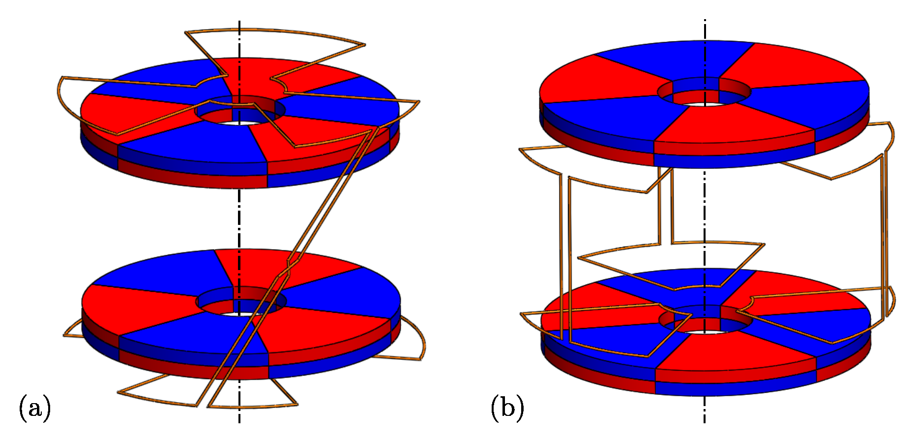
The thrust bearing being analysed is constituted of two independent subassemblies, namely the PM arrangements and the armature winding, in rotary motion relative to each other, as illustrated in
Figure 1. Each of them can be attached either to the stator or to the rotor.
The first subassembly comprises two PM arrangements, each producing an identical axial magnetic field with p pole pairs. These arrangements can:
either be placed in repulsive or attractive mode, as represented in
Figure 1; and
either constitute the internal or external subassembly, as shown in
Figure 1a,b respectively.
The armature winding comprises N identical and evenly distributed phase windings. The latter are each constituted of two identical sets of p identical and evenly distributed coils, each set being predominantly magnetically linked to one PM arrangement, and can be of two types:
the
p coils of each set are connected in series, the two resulting sets being connected together, as illustrated in
Figure 1a;
the
p upper and the
p lower coils are independently connected together, as represented in
Figure 1b.
Besides, as illustrated in
Figure 1a,b, respectively, both upper and lower sets of coils can be shifted by an angle equal to
or zero and can be connected either in series or in opposition. This connection is chosen on the basis of the angular shift that separates the upper and lower sets as well as the attractive or repulsive mode of the PM arrangements so as to ensure that the flux linked by the armature winding is null when the rotor is axially centred with respect to the stator, thereby respecting the null-flux principle.
3. Electromechanical Model
Under the assumption of small rotor axial, radial and angular displacements and neglecting the inductance coefficient variations with these displacements, the axial dynamics of the system constituted of the rotor and the ETDB is decoupled from the radial and angular ones [
22]. Assuming in addition that the rotor spin speed varies slowly compared to the axial dynamics, the latter can be described through a linear state-space representation as extensively derived in [
18]:
with:
where
z and
are, respectively, the rotor axial position and velocity;
F and
T are, respectively, the electrodynamic force and torque;
is the external axial force acting on the rotor;
C is the external non-rotating damping;
M is the rotor mass;
R is the phase winding resistance;
is the cyclic inductance, thus taking into account the self and mutual inductance coefficients of the
N phases constituting the armature winding;
is the proportionality factor between the amplitude of the flux linked by the phase windings due to the PMs and the axial position; and
is the external axial stiffness. The latter could, for example, arise from detent effects or be related to the axial stiffness induced by centring PM bearings added to the system so as to ensure the rotor radial and angular guidance. Hence, this stiffness is generally negative, as it is assumed hereafter.
Assuming quasi-static conditions, i.e.,
, the axial electrodynamic stiffness
as well as the associated braking torque
can be retrieved from this dynamic model, yielding [
18]:
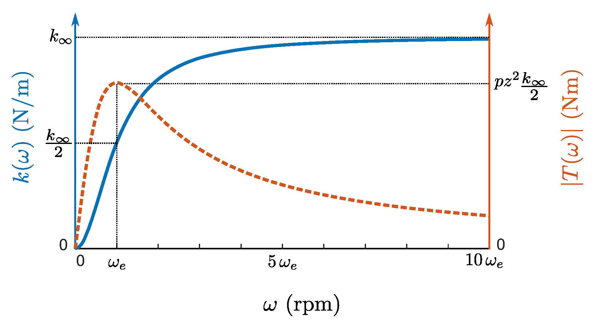
As depicted in
Figure 2, illustrating the evolution of the stiffness, the latter increases with the spin speed and can be characterised through two coefficients, namely the rotor spin speed
related to the electrical pole and the asymptotic stiffness
, defined as:
The latter therefore corresponds to the maximal axial stiffness that can be generated by the EDTB. Let us point out that this stiffness appears explicitly in the state matrix
, given in Equation (2). On the contrary, as shown in
Figure 2, the braking torque
reaches its maximal value when the speed is equal to
and then decreases asymptotically to zero.
4. Stability Analysis
The behaviour of EDTBs is strongly dependent on the rotor spin speed and so is their stability. Hereinafter, general considerations about the stability of an EDTB coupled to the rotor are first derived. On this basis, the static and dynamic stability are then analysed, leading to conditions ensuring a stable behaviour at a specific rotor spin speed.
The following developments can be greatly simplified by considering the electrical pole as being much greater than the maximal natural frequency of the equivalent spring–mass system constituted of the rotor and the EDTB:
In this way, the electrical phenomena are much faster than the mechanical ones and thus do not have a significant impact on the rotor axial dynamics. Observing that the electromechanical model, given in Equation (
1), depends on the stiffness as well as the rotor mass and not their square roots, Equation (6) can be expressed in a more convenient manner as:
To the authors’ best knowledge, the latter hypothesis is verified in the vast majority of the experimental and numerical studies of EDTBs, including the case study in
Section 7. In addition, let us assume a priori that the external damping satisfies:
This assumption is verified a posteriori in
Section 4.3.
4.1. General Considerations
The model in Equation (
1) being linear, the stability analysis can be performed through the study of the real part of the four eigenvalues of the state matrix
as a function of the spin speed. To this end, the characteristic polynomial can be easily derived, yielding:
Under the hypothesis expressed in Equation (7) and assuming Equation (8) as verified, the polynomial in Equation (9) can be simplified as follows:
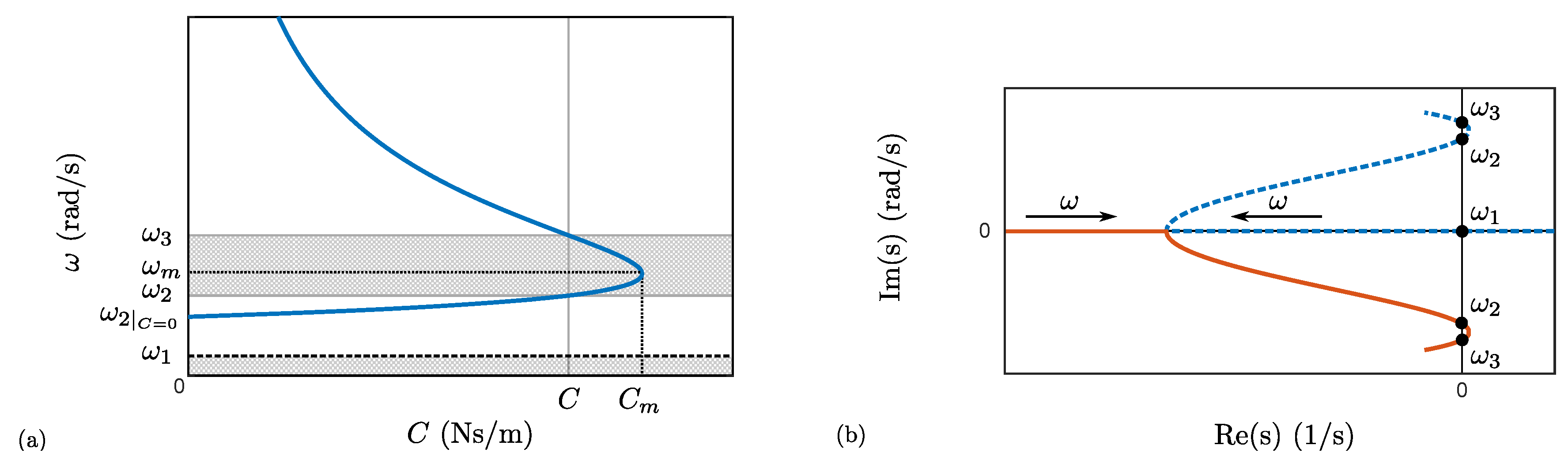
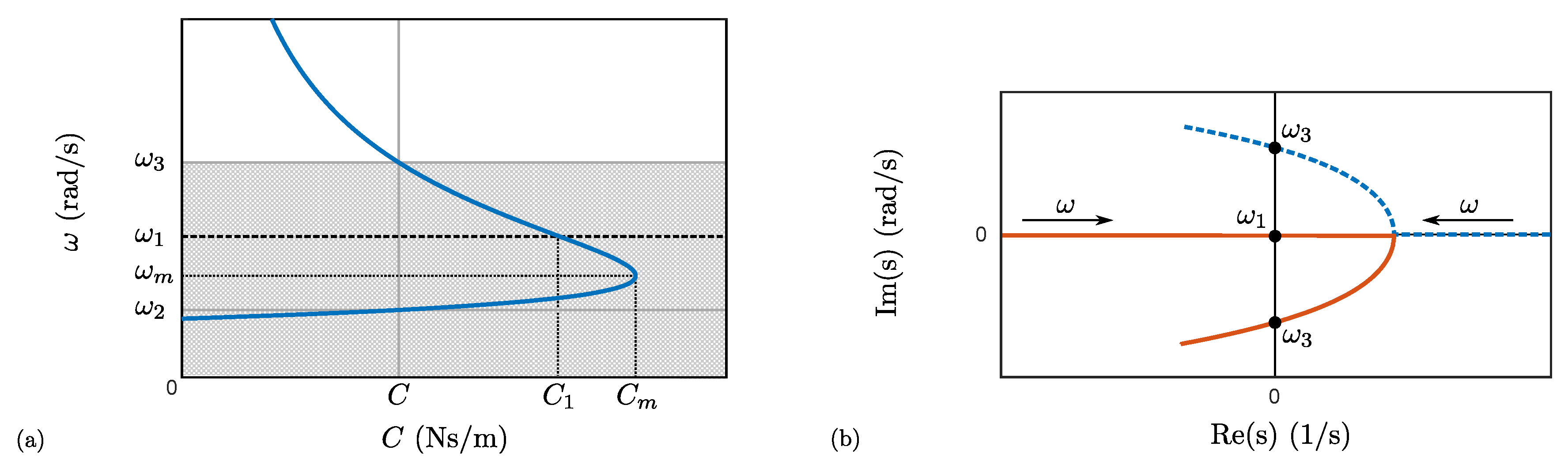
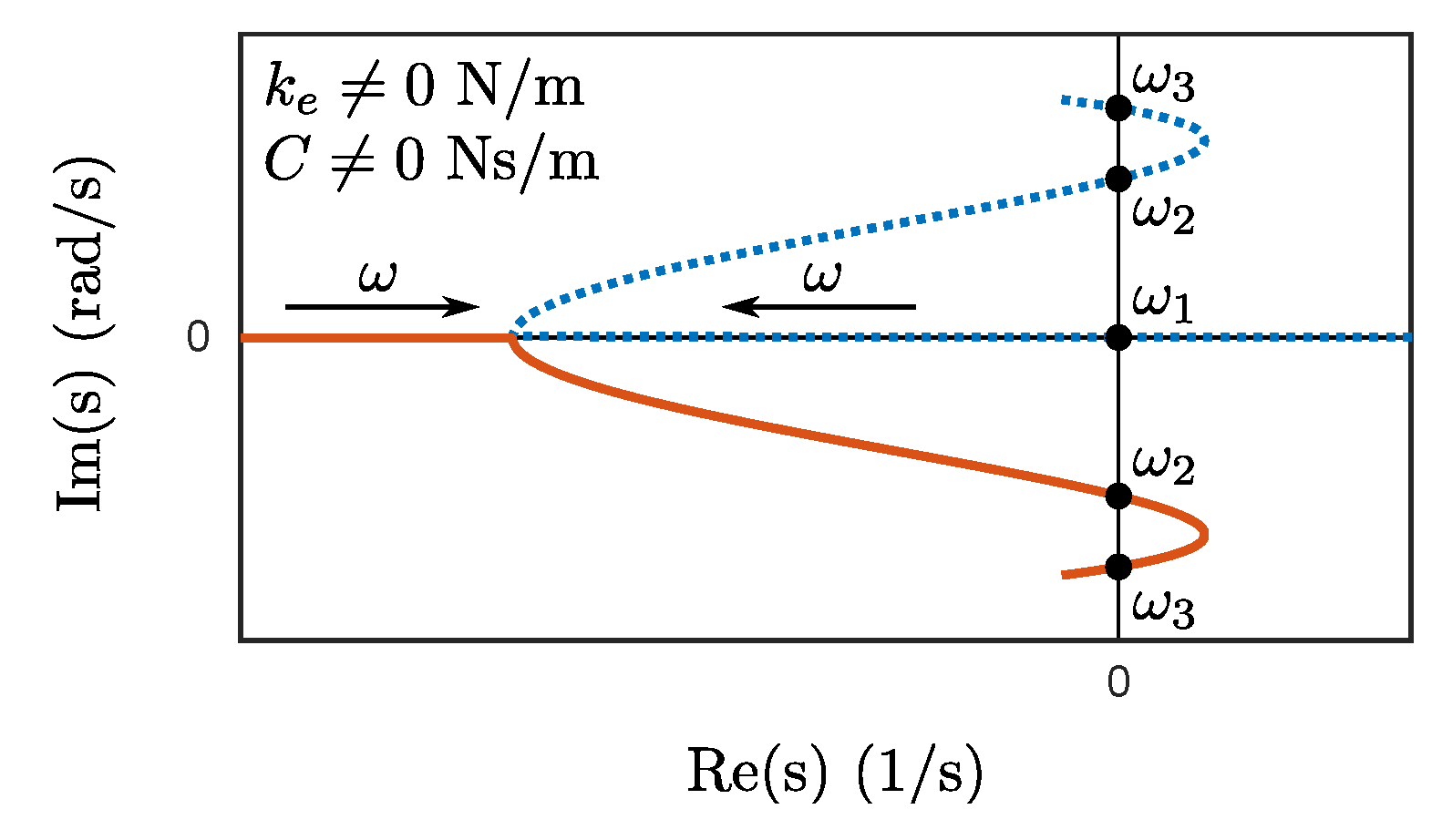
The root locus of the four eigenvalues can thus be obtained by finding the roots of Equation (10) for different spin speeds. However, when it comes to stability analyses, only the speeds at which the eigenvalues cross the imaginary axis are relevant as they define the spin speed ranges within which the bearing is stable.
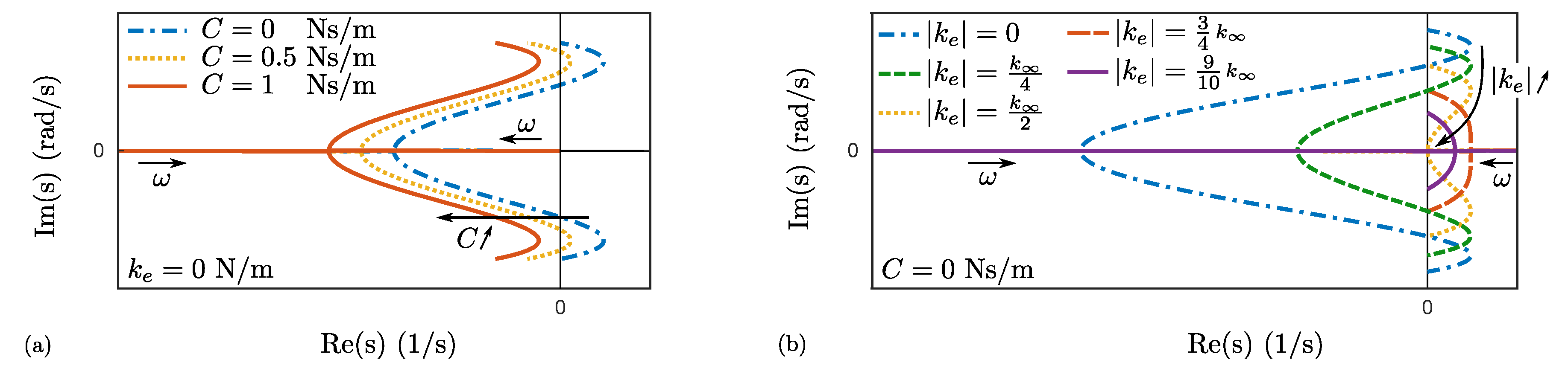
Figure 3a,b illustrates, respectively, the impact of the external damping and stiffness on the root locus. Only the two relevant eigenvalues, related to the mechanical behaviour, are represented, the remaining two, related to the electrical behaviour, being located far in the left half plane. The additional damping allows us to shift the complex conjugates parts of the root locus to the left by an amount equal to
, whereas the external stiffness strongly modifies their shape.
As a result, there are at most three spin speeds,
,
and
, defined in
Figure 4, corresponding to intersections with the imaginary axis. More precisely, as shown in
Figure 3, when the external damping approaches zero, the spin speed
tends to infinity and therefore no longer exists. By contrast, increasing the damping allows us to move the spin speeds
and
towards each other until they are equal, when the damping reaches a specific value, denoted by
hereinafter. Beyond the latter damping, these two speeds do not exist anymore. Besides, as illustrated in
Figure 3b, the presence of the speed
strongly depends on the external stiffness.
For determining these speeds, let us assume that
, implying that the eigenvalue lies on the imaginary axis. In this case, Equation (10) can be separated into real and imaginary parts as follows:
Solving Equation (12) for h yields three solutions. As demonstrated hereinafter, one solution is related to a static instability, whereas the other two are linked to a dynamic one.
4.2. Static Stability
The trivial solution of Equation (12), i.e.,
, corresponds to the first intersection of the eigenvalues with the imaginary axis. Substituting this solution into Equation (11) and isolating
leads to:
This corresponds to the spin speed at which the stiffness induced by the electrodynamic effects exactly compensates for the external stiffness, i.e.,
, as can be verified through Equation (4). Below this specific spin speed, the thrust bearing suffers from an instability as the external stiffness, whose effect is destabilising due to its negative value, is larger than the electrodynamic one. This instability can be qualified as static as it does not depend on the damping. The static stability condition can thus be stated as:
Two limiting cases can be studied. On the one hand, when there is no external stiffness, the speed is equal to zero and the static stability condition does not introduce any restriction on the rotor spin speed. On the other hand, when the external stiffness is larger, in absolute value, than the maximal electrodynamic stiffness, i.e., , the speed tends to infinity and the bearing is unstable regardless of the rotor spin speed.
4.3. Dynamic Stability
Both remaining solutions of Equation (12) are linked to a dynamic instability as they depend on the damping. They can be calculated as follows:
Substituting Equation (15) into Equation (11) and multiplying by
yields:
where:
The polynomial in Equation (16) has at most two positive roots, thereby confirming that both eigenvalues related to the electrical behaviour never cross the imaginary axis. Under the hypothesis expressed in Equation (7) and still assuming that the damping satisfies Equation (8), the coefficients in Equation (17) can be greatly simplified, leading to:
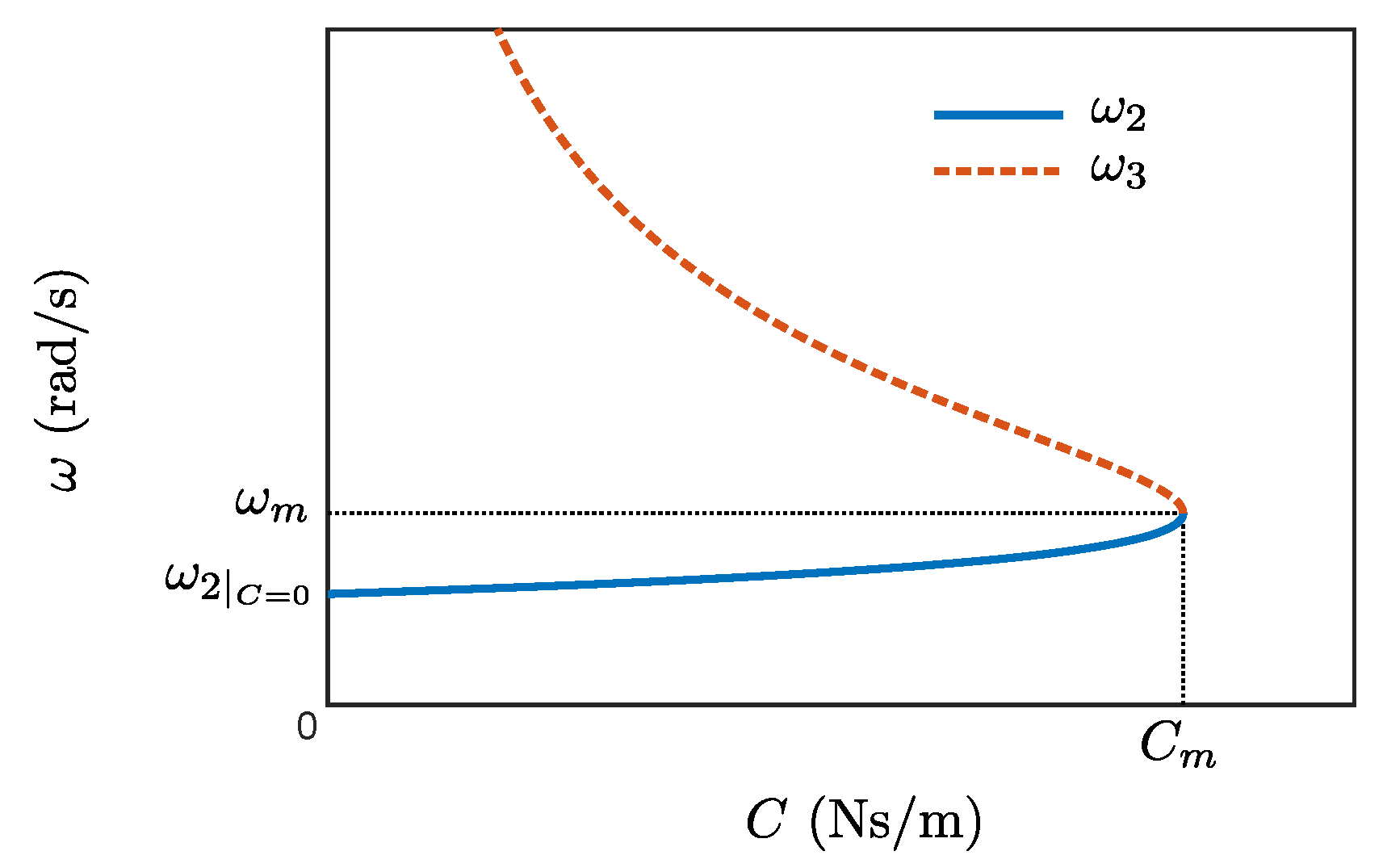
Solving Equation (16) with these reduced coefficients allows us to determine both spin speeds
and
at which the relevant eigenvalues cross the imaginary axis, as shown in
Figure 4:
The value of these speeds is independent from the external stiffness
, signifying that the intersections of the eigenvalues with the imaginary axis occur at the same spin speeds even when the shape of the root locus is modified by this stiffness, as shown in
Figure 3b. By contrast, as mentioned in
Section 4.1, the existence of these intersections strongly depends on the external damping and stiffness.
Figure 5 shows the evolution of both speeds
and
with the external damping. As expected, when the latter is equal to zero, the speed
tends to infinity and therefore no longer exists, whereas the speed
can be easily calculated by observing that the coefficient
in Equation (18) is equal to zero, implying that Equation (16) has only one positive solution:
This speed thus corresponds to spin speed
related to the electrical pole. Let us point out that spin speeds smaller than this particular speed can never lie on the imaginary axis and are therefore stable, from a dynamic point of view, regardless of the damping. As stated in
Section 4.1, adding external damping enables moving the speeds
and
towards each other until they intersect, when the damping reaches
. Cancelling the coefficient
in Equation (21) allows us to determine both the damping
such that these two speeds are equal and the corresponding speed, denoted by
:
Below this damping, the speeds
and
are distinct and the EDTB is unstable, from a dynamic point of view, when the spin speed belongs to the interval
, as shown in
Figure 4. By contrast, when the damping is larger than
, the eigenvalues only cross the imaginary axis at the speed
and the EDTB is stable beyond the latter speed. Consequently, unlike their static counterparts, dynamic instabilities can be removed through additional non-rotating damping.
Finally, substituting the maximal damping given in Equation (23) into Equation (8) and considering that the assumption in Equation (7) is verified allows us to validate the relation in Equation (8) a posteriori, highlighting that the latter is not, as such, a hypothesis.
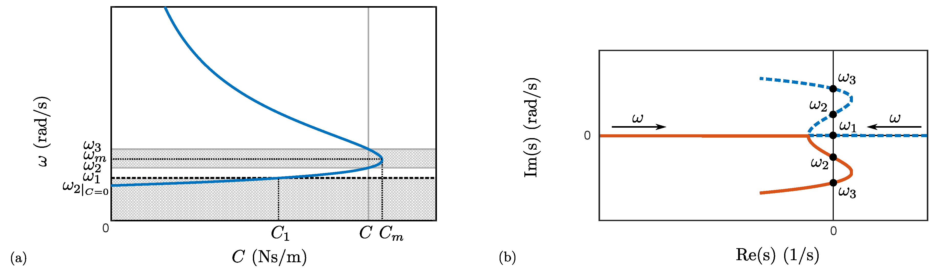
4.4. Stability Conditions
In summary, the stability can be analysed on the basis of:
the speed related to the static instability, given in Equation (13);
the speeds and , related to the dynamic instability, as a function of the damping, defined in Equation (21); and
the external damping C added to the system.
More precisely, when the maximal electrodynamic stiffness is larger than the external one, i.e.,
, the stability is ensured at the spin speed
provided that:
Finally, let us point out that the state-space representations in [
17,
21] yield an identical characteristic polynomial to Equation (9), thus widening the scope of the previous developments to these models.
7. Case Study
The case study was performed on the three EDTBs illustrated in
Figure 9. The first corresponds to a topology with a merged armature winding as internal subassembly and is denominated Topology 1. The second bearing, denominated Topology 2, corresponds to the topology with two distinct PM arrangements as internal subassembly and the armature winding consisting of two sets of
p coils connected in series, the two resulting sets being themselves connected in opposition. The last one, denominated Topology 3, is identical to the second but includes in addition back irons on which the sets of coils are placed. In each of these three topologies, the PM arrangements comprise ferromagnetic yokes, the remanent magnetisation is 1.42 T and the number
p of pole pairs is two. The armature winding comprises three phases (
) and the conductor density, defined as the number of conductors per unit of coil section, is 4 per square millimetre. The rotor includes the armature winding and its mass was set to 1 kg. Lastly, the overall dimensions of the three topologies, given in
Table 3, are identical and so is their PM volume.
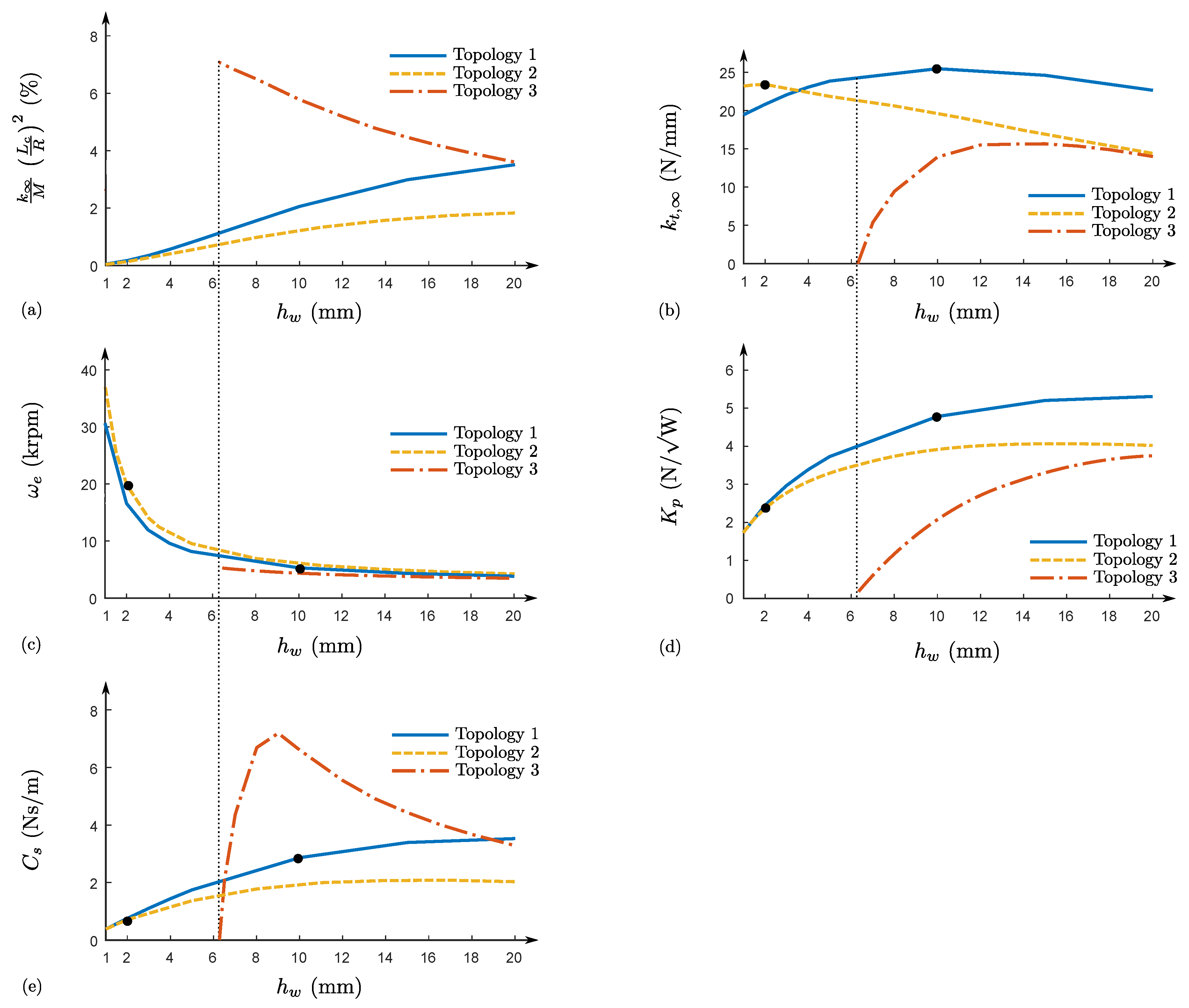
7.1. Parametric Analysis
For each topology, a parametric analysis of the four performance criteria defined above was performed with respect to the winding thickness
. To this end, the model parameters were identified for all configurations through static finite element simulations by applying the methods detailed in [
18]. As illustrated in
Figure 10a, the square of the ratio between the natural frequency of the equivalent spring–mass system and the electrical pole stayed below 7%, therefore validating the assumption in Equation (7) as well as the resulting developments with regard to the stability analyses and the external damping required to stabilise the bearing.
Figure 10b shows the evolution of the maximal total stiffness with the winding thickness. Topology 1 reached its maximum, namely 25.5 N/mm, when the thickness was equal to 10 mm, whereas Topology 2 had a peak value of 23.5 N/mm for a thickness of 2 mm. Furthermore, below a thickness of about 6.2 mm, represented by a dotted line, the total stiffness of the third topology was negative, meaning that the detent force due to the interaction between the PMs and the back irons was larger than the electrodynamic one and thus leading to a static instability regardless of the speed. Above this particular thickness, the maximal stiffness increased until it joined the curve related to Topology 2 without ever exceeding the latter. The presence of the back irons is therefore clearly not advantageous as regards the axial stiffness.
Figure 10c shows the evolution of the spin speed
corresponding to the electrical pole with the winding thickness. Regardless of the latter, Topology 1 showed smaller speeds
than Topology 2, signifying that the stiffness reached its maximum at lower speeds. However, the discrepancy between these two topologies decreased with the thickness. As regards Topology 3, as soon as the total stiffness became positive, the electrical pole remained smaller than the one related to Topology 2 given that the back irons allows us to increase the cyclic inductance
while maintaining the resistance
R unchanged.
Figure 10d shows the evolution of the energy efficiency coefficient
with the winding thickness. As regards this criterion, Topologies 1 and 2 were rather close for small thicknesses. However, the former always outclassed the latter and the gap widened with the winding thickness. In comparison with these two topologies, the efficiency of Topology 3 remained quite low due to the negative contribution of the axial detent force.
Figure 10e shows the evolution of the damping required to stabilise the bearing at high speeds with the winding thickness. As mentioned in
Section 6.3, the damping related to the Topologies 1 and 2 presented an identical shape to the curves linked to the energy efficiency, given that the latter is proportional to the square root of the required damping in the absence of external stiffness. More precisely, it remained limited to relatively small values, namely no more than 2.0 and 3.5 Ns/m, respectively. By contrast, Topology 3 required slightly larger damping with up to the double, i.e., 7.2 Ns/m.
In summary, Topology 1 is attractive for a winding thickness close to 10 mm as the stiffness
is maximal, whereas the spin speed related to the electrical pole is rather low, namely 5200 rpm. Besides, the energy efficiency coefficient is important and the required damping, being equal to 2.9 Ns/m, can be considered as reasonable in light of the values reported in the literature [
23]. Topology 2 with a winding thickness equal to 2 mm yields an almost equivalent maximal stiffness, although the electrical pole is about four times larger. The required damping is thus smaller for this topology, being equal to 0.71 Ns/m, and therefore easier to produce. However, it also means that the energy efficiency is reduced by a factor about 2. Let us point out that, without considering the distance
l between both parts of Topology 2, the volume occupied by both topologies is nearly identical. Only Topologies 1 and 2 with a winding thickness equal to 10 and 2 mm, respectively, were further considered.
7.2. Rotational Losses
Assuming a constant external force
, the resulting axial displacement can be determined through Equation (
1) as well as Equation (4) and then substituted into Equation (31) giving the rotational losses, yielding:
Considering the rotor weight as external load, namely approximately 10 N, the minimal rotational losses , given in Equation (35), were, respectively, equal to 4.4 and 17.8 W for Topologies 1 and 2. Topology 1 therefore dissipated about four times less power for an identical load. Indeed, in the absence of external stiffness, these losses were inversely proportional to the damping required to stabilise the thrust bearing regardless of the spin speed.
7.3. Stiffness Analysis
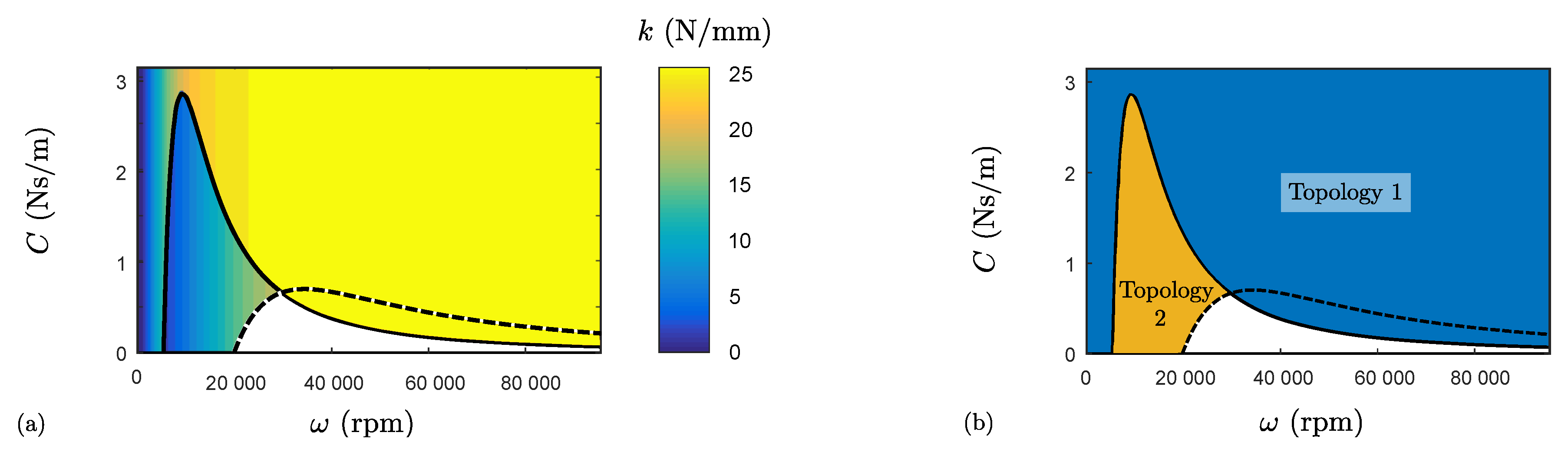
We studied the evolution of the stiffness with the rotor spin speed for Topologies 1 and 2.
Figure 11a,b represents, respectively, while taking into account the stability conditions for each spin speed and amount of external damping, the maximal stiffness among both topologies and the corresponding topology. The solid and dashed lines illustrate, respectively, the stability boundary related to Topologies 1 and 2, the latter being defined as the evolution with the damping of the speeds
given in Equation (21). In this way, below each curve, the corresponding topology suffers from a dynamic instability, also implying that both are unstable in the white zone.
Regardless of the spin speed, Topology 1 provided a higher stiffness and reached its maximal stiffness
for lower speeds than Topology 2 given that the electrical pole was smaller. By contrast, in the absence of additional damping, Topology 1 was also unstable for a smaller speed. Indeed, as stated in
Section 6.1, minimising the spin speed
related to the electrical pole amounts to reducing the stable speed range when there is no external damping. Therefore, between about 5000 and 20,000 rpm, namely the spin speeds related to the electrical poles of both topologies, Topology 2 offers the major advantage of not requiring external damping to ensure the axial stable levitation of the rotor. This brief analysis shows that the rotor spin speed can still strongly influence the bearing selection according to the application specifications.
8. Conclusions
This paper presents four criteria allowing us to compare objectively various electrodynamic thrust bearing topologies based on their intrinsic qualities and therefore to determine the most appropriate.
On the basis of the recent linear state-space representations describing the axial dynamics of EDTBs, an analytical static and dynamic stability analysis is performed through the calculation of the eigenvalues of the state matrix. The impact of the external damping and stiffness is studied through a root locus as a function of the rotor spin speed, highlighting that the former allows us to move the eigenvalues to the left, thus improving the stability, whereas the latter modifies their shape. Besides, the spin speeds corresponding to intersections with the imaginary axis are calculated, therefore defining the ranges within which the thrust bearing is stable. In the absence of additional damping and external stiffness, the thrust bearing is stable up to the spin speed related to the electrical pole.
When it comes to comparing magnetic bearings, the maximal eccentricity, the losses and the stability are of primary interest. As a result, the following four performance criteria are defined: (i) the maximal total stiffness; (ii) the spin speed corresponding to the electrical pole; (iii) the levitation energy efficiency, defined as the ratio between the thrust force and the corresponding rotational losses; and (iiii) the damping required to stabilise the bearing regardless of the rotor spin speed. Three different thrust bearing topologies, studied in the framework of a case study, are finally compared on the basis of these criteria, notably highlighting that the addition of back irons behind the sets of coils has no beneficial effect as regards axial dynamics due to the important detent stiffness.


