Offset-Free Model Predictive Control for Active Magnetic Bearing Systems

Abstract

This paper presents the study of linear Offset-Free Model Predictive Control (OF-MPC) for an Active Magnetic Bearing (AMB) application. The method exploits the advantages of classical MPC in terms of stability and control performance and, at the same time, overcomes the effects of the plant-model mismatch on reference tracking. The proposed approach is based on a disturbance observer with an augmented plant model including an input disturbance estimation. Besides the abovementioned advantages, this architecture allows a real-time estimation of low-frequency disturbance, such as slow load variations. This property can be of great interest for a variety of AMB systems, particularly where the knowledge of the external load is important to regulate the behavior of the controlled plant. To this end, the paper describes the modeling and design of the OF-MPC architecture and its experimental validation for a one degree of freedom AMB system. The effectiveness of the method is demonstrated in terms of the reference tracking performance, cancellation of plant-model mismatch effects, and low-frequency disturbance estimation.

1. Introduction

The adoption of Active Magnetic Bearings (AMBs) in industrial applications has exhibited a steady growth in the last decades because of their remarkable advantages over traditional oil-lubricated bearings due to their contactless nature. This allows tribology and fatigue issues to be avoided, reducing power losses and eliminating oil supply units. Furthermore, AMB systems are characterized by monitoring and diagnostic capabilities, while the high tunability of the control action permits on-line adjustments of the bearing system according to the operating conditions. These and other benefits have favoured the adoption of AMBs in a variety of applications such as kinetic energy storage systems, the oil & gas and vacuum industry, heart pumps, refrigeration compressors and milling spindles [1,2,3].

Nowadays, the research effort to refine this technology is focused on several aspects, such as actuator configuration [4,5,6], sensing technology [7,8,9], the interaction with rotordynamic aspects [10,11], and the integration of an electric motor with magnetic bearings [12,13]. The control strategy is typically based on linear or nonlinear control architectures like PID, H∞, $\mu$-synthesis, sliding mode control, LQ, and learning control [14,15,16,17,18]. Each of these strategies has the main goal of compensating for the inherent unstable behaviour of the system and satisfying the demands of performance, robustness, and accuracy. In this scenario, Model Predictive Control (MPC) has gained increasing attention in the last few years and has been implemented in a variety of applications and in different forms to tackle issues of nonlinearities and variability of the operating conditions. A rich literature describes the potentialities of this approach in magnetic levitation [19,20,21,22,23]. In particular, MPC has shown an improved performance in compensating for gyroscopic effects [24] and revealed properties of good stability and robustness when compared with standard control architectures for the levitation of flywheels [25]. When using MPC for AMBs, the electromagnets’ current reference is obtained by solving a finite horizon open-loop optimal control problem either in real-time or offline. The current state of the plant is considered as the initial state at every step of computation. If the actual process and the nominal model match perfectly, this control scheme ensures the stability and allows the tracking of any reachable target without offset. Nevertheless, in AMB systems, the perfect match between plant and model is rather difficult to obtain, mainly because of nonlinear effects that are present in the magnetic actuators [26] and uncertainty in the model parameters [27]. Increasing the model complexity may not be enough to overcome this issue due to the intrinsic difficulty in evaluating or identifying all unknown model parameters. This leads to an almost unavoidable steady-state offset of the closed loop system. The inclusion of some form of integrative action in the MPC scheme is therefore required to yield Offset-Free Model Predictive Control (OF-MPC). Different approaches have been proposed in the literature to obtain OF-MPC: (a) adding an external integrative action to the tracking error [22]; (b) completing the cost function of the MPC scheme with a term related to the tracking error [28]; (c) adopting the so-called “velocity form linear model” considering the variations between two time-steps of the input and, if needed, of the state [29]; and (d) exploiting a disturbance observer based on an augmented plant model. The last case can be performed with either an “output disturbance model” [30] or an “input disturbance model” [31,32]. In the last years, these techniques have been intensively studied in terms of their linear and nonlinear formulations [31,32,33,34,35,36], as well as in terms of their applications in a variety of real cases. They have shown advantageous properties of stability and robustness [37,38,39]. To the authors’ knowledge, linear OF-MPC based on an “input disturbance model” has not been attempted yet in AMB systems, despite its inherent capability to handle the steady-state offset generated by the plant-model mismatch and by unmeasured nonzero-mean disturbances. Hence, this is the objective of the present study. An additional advantage of the proposed method is to allow a real-time estimation of the low-frequency external disturbances and load variations acting on the AMB system to be obtained. This property is of great importance in applications such as compressors, pumps, and blowers, where the axial load applied to the machine can change significantly according to the operating conditions. Finally, a non-negligible additional benefit of the proposed architecture is related to the adoption of the Kalman filter, which, besides estimating the disturbance force, provides a cleaner estimation of displacement and velocity, thus reducing the influence of the noise affecting the sensor signals.

The proposed technique is tested on a single-degree-of-freedom AMB system actuated by means of a couple of electromagnets. The modelling of the system is described together with the design of the OF-MPC in all its parts: general control architecture, disturbance model and observer design, target calculation, and MPC problem formulation. The experimental results demonstrate the effectiveness of the proposed approach in terms of the reference tracking performance and real-time estimation of the low-frequency external load in comparison with standard MPC.

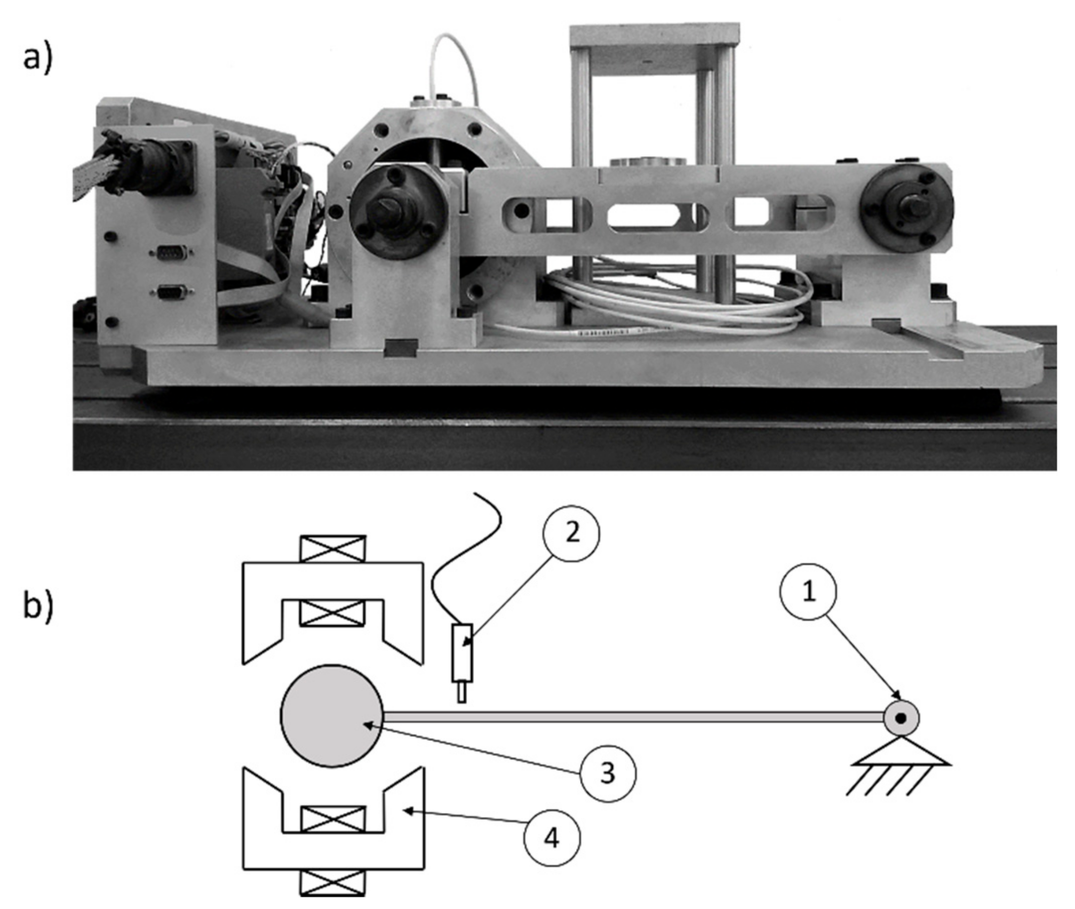
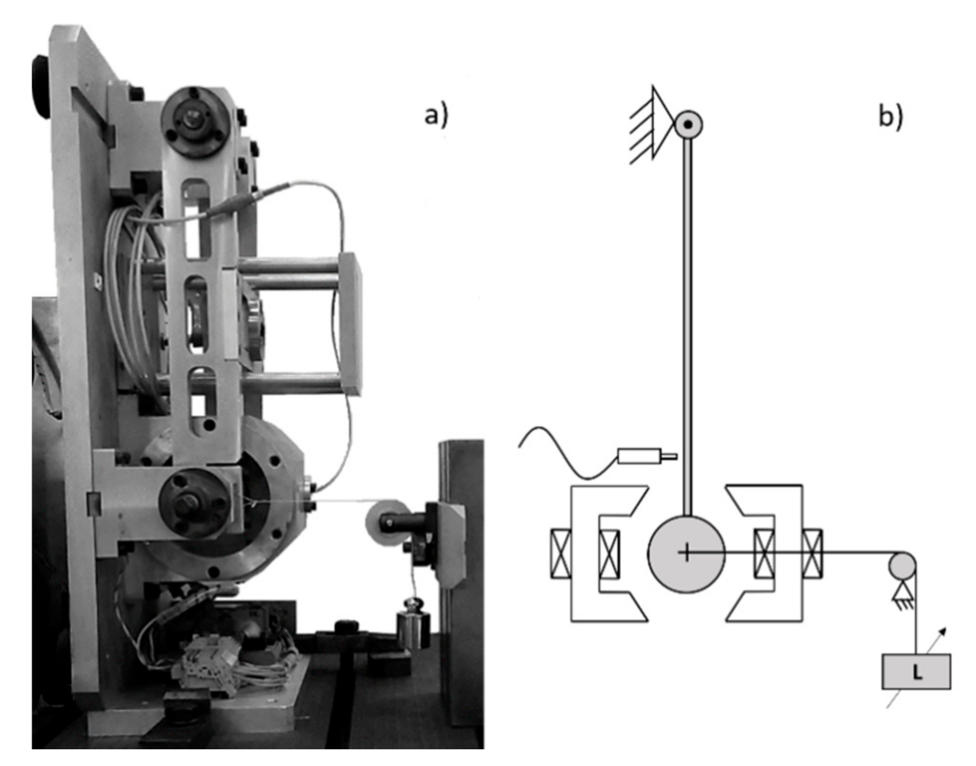
2. Single Degree of Freedom Active Magnetic Bearing System

The test rig adopted for the experimental validation is a single-degree-of-freedom AMB system presented in Figure 1. It consists of a horizontal arm hinged at one extremity with a pivot and controlled at the other extremity by means of a single-axis magnetic bearing with two opposite electromagnets.

The length of the arm (320 mm) and the small airgap (0.6 mm) ensure that the circular motion of the mass can be approximated with a pure linear displacement ($q$). The base plate, connecting the arm and electromagnets’ housing, is made from aluminium, and the shaft is steel, while silicon iron laminations are used for the stator and moving part of the magnetic circuit. The displacement of the mass is detected by means of a Bently Nevada Proximitor 3300XL (Minden, NV, USA) eddy current sensor. The currents in the electromagnets are measured by two AMP25 Hall sensors, one per electromagnet. The main electro-mechanical parameters of the plant are listed in

Table 1. Plant parameters.

Symbol	Name	Value	Unit
$m$	Mass	$3.41$	$\mathrm{kg}$
$S$	Cross-section area at the air gap	$420$	${\mathrm{mm}}^2$
$q_0$	Nominal airgap	$0.6$	$\mathrm{mm}$
$n$	Number of turns	$142$	-
$R$	Coil resistance	$0.35$	$\mathrm{Ohm}$
$L_0$	Coil nominal inductance	$5.8$	$\mathrm{mH}$
$k_i$	Current-force factor	$13.65$	$\mathrm{N}/\mathrm{A}$
$k_q$	Electromagnet negative stiffness	$11.4$	$\mathrm{N}/\mathrm{mm}$
$k_m$	Back-electromotive-force factor	$13.65$	$\mathrm{Vm}/\mathrm{s}$

.

A dSPACE MicroLabBox unit is used to close the feedback loop and for data acquisition. It includes a Freescale QorlQ P5020 real-time processor and a FPGA-PC-dSPACE prototyping platform for rapid control software development. The power stage consists of an H-bridge for each electromagnet with a $20 \mathrm{kHz}$ fixed PWM frequency and a $24 \mathrm{V}$ DC bus voltage.

3. Modeling

As is usual in AMB systems, the two electromagnets are operated in differential driving modes, i.e., one electromagnet is driven with the sum of bias and control current $\left(i_0+i_c\right)$, while the other one with their difference $\left(i_0-i_c\right)$. In the closed loop, $i_c$ is set by the position controller, while $i_0$ is fixed. The system dynamic equilibrium equation is

$$m\dot{v} = f_m\left(i_c,q\right)+f_d$$

(1)

where $m$ is the equivalent mass of the moving parts (including the arm and the moving part of the magnetic circuit) $v$ is its velocity, $f_m$ represents the magnetic actuators’ force, and $f_d$ represents an external disturbance force.

Assuming that: the two electromagnets are identical and magnetically uncoupled with each other, no saturation occurs in the magnetic material, the stray flux and eddy current effect are negligible, and the reluctance in the ferromagnetic part is negligible compared to that of the (small) air gap, the nonlinear magnetic force can be expressed as

$$f_m\left(i_c,q\right)=\Gamma \left(\frac{{\left(i_0+i_c\right)}^2}{{\left(q_0-q\right)}^2}-\frac{{\left(i_0-i_c\right)}^2}{{\left(q_0+q\right)}^2}\right)\cos \alpha$$

(2)

where coefficient $\Gamma = {\mu }_0{n}^{2}S$ includes the number of coils $n$, the cross-section area of the air gap $S$, and the magnetic permeability of the vacuum ${\mu }_0 = 1.26 \times {10}^{-6} \mathrm{N}/{\mathrm{A}}^2$ [1]. The error of the predicted force with this modeling approach is within a range of 5%–10% ([1] Section 3.1.5). $\mathsf{\alpha } = 22.5°$ is the angle of each pole relative to the centerline between the poles.

In linear AMB, the nonlinear function of (2) is linearized at the operating point with nominal airgap $q_0$, as

$$f_m\left(i_c,q\right) = k_i{i}_c+k_{q}q$$

(3)

where $k_i$ and $k_q$ are the force-current and force-displacement (or negative stiffness) factors, respectively. The linearization of (3) makes the control design easier as it can exploit all tools of linear control theory. Nevertheless, it becomes the first cause of plant-model mismatch, as well as the aforementioned assumptions at the base of the force Equation (2). These effects lead to a mismatch of the actual $k_i$ and $k_q$ coefficients relative to their nominal value and the force in Equation (3) can be rewritten as

$$f_{m,real}\left(i_c,q\right) = \left(k_i+{\xi }_i\right)i_c+\left(k_q+{\xi }_q\right)q$$

(4)

where ${\xi }_i$ and ${\xi }_q$ are the uncertainty on current-force and force-displacement factors, respectively. If the uncertainty is constant as time tends to infinity, (4) becomes

$$f_m^{*}{\left(i_c,q\right)}_{\infty } = k_i{i}_{c,\infty }+k_q{q}_{\infty }+\xi$$

(5)

where $\xi$ stands for the uncertainties of the force factors due to plant-model mismatch.

The plant-model mismatch and low-frequency external disturbance effects can be combined into one disturbance term as

$$d\left(t\right) = \xi +f_d\left(t\right)$$

(6)

The augmented model at the base of the OF-MPC controller is given by (1), (3), and (6), and can be expressed with the linear continuous-time state space representation

$$\begin{array}{l}\dot{x}\left(t\right) = \left[\begin{array}{cc}0& 1\\ \frac{k_q}{m}& 0\end{array}\right]x\left(t\right)+\left[\begin{array}{c}0\\ \frac{k_i}{m}\end{array}\right]u\left(t\right)+\left[\begin{array}{c}0\\ \frac{1}{m}\end{array}\right]d\left(t\right)\hfill \\ y\left(t\right) = \left[\begin{array}{cc}1& 0\end{array}\right]x\left(t\right),\hfill \end{array}$$

(7)

where $u$ stands hereinafter for the control current $i_c$, and the state vector includes the displacement $q\left(t\right)$ and the velocity $v\left(t\right)$ of the moving mass.

$$x\left(t\right) = {\left[q\left(t\right),v\left(t\right)\right]}^T$$

(8)

The method exploits a discrete, linear time-invariant model derived from (7).

$$\begin{array}{l}X\left(k+1\right) = Ax\left(k\right)+Bu\left(k\right)+B_{d}d\left(k\right)\hfill \\ y\left(k\right) = Cx\left(k\right)\hfill \end{array}$$

(9)

Aiming to obtain an offset-free control in the controlled variable $y$, a disturbance model is required to reject unmeasured low-frequency disturbances caused by plant-model mismatch or from external loads. To this end, the plant model (9) is augmented with a disturbance state:

$$\begin{array}{l}\left[\begin{array}{c}x\left(k+1\right)\\ d\left(k+1\right)\end{array}\right] = \left[\begin{array}{cc}A& B_d\\ 0_{1x2}& 1\end{array}\right]\left[\begin{array}{l}x\left(k\right)\hfill \\ d\left(k\right)\hfill \end{array}\right]+\left[\begin{array}{c}B\\ 0\end{array}\right]u\left(k\right)+\left[\begin{array}{c}{w}_x\left(k\right)\\ w_d\left(k\right)\end{array}\right]\hfill \\ y\left(k\right) = \left[\begin{array}{cc}C& C_d\end{array}\right]\left[\begin{array}{c}x\left(k\right)\\ d\left(k\right)\end{array}\right]+w_n\left(k\right)\hfill \end{array}$$

(10)

where $d$ is the disturbance of (6), $w_x\in {\mathbb{ℝ}}^2$ and $w_d\in \mathbb{ℝ}$ represent the state noise, and $w_n\in \mathbb{ℝ}$ is the output noise. Matrices $B_d$ and $C_d$ represent the effect of the disturbance $d$ on the state and output equations, respectively. If only the disturbance on the output is considered, then $B_d$ is a zero matrix and $C_d$ is nonzero, the integrating disturbance $d$ is only added to the output $y$, and the resulting formulation is therefore called the output disturbance model. By converse, considering the interest in turning $d$ into a representation of plant-model mismatch and external disturbance force, the disturbance will not have a direct influence on the output equation (i.e., $C_d = 0$) and the resulting augmented model is called the input disturbance model with $B_d \ne 0$. In this last case, the output equation in (10) is not affected by the disturbance $d$:

$$y\left(k\right) = Cx\left(k\right)+w_n\left(k\right)$$

(11)

Provided that the system (9) is observable ($\left(C,A\right)$ has full rank) and also (10) is observable, as witnessed by the full rank of matrix

$$rank\left(\left[\begin{array}{cc}A-I& B_d\\ C& C_d\end{array}\right]\right) = p + 1$$

(12)

where $p = 2$ is the number of the states, then the state and the disturbance are estimated by

$$\left[\begin{array}{c}\widehat{x}\left(k+1\right)\\ \widehat{d}\left(k+1\right)\end{array}\right] = \left[\begin{array}{cc}A& B_d\\ 0& I\end{array}\right]\left[\begin{array}{c}\widehat{x}\left(k\right)\\ \widehat{d}\left(k\right)\end{array}\right] + \left[\begin{array}{c}B\\ 0\end{array}\right]u\left(k\right) +\left[\begin{array}{c}{L}_x\\ L_d\end{array}\right]\left(-y\left(k\right)+C\widehat{x}\left(k\right)\right)$$

(13)

where $L_x\in {\mathbb{ℝ}}^2$ and $L_d\in \mathbb{ℝ}$ are the predictor gain matrices for the state and the disturbance, respectively. They are calculated off-line, solving the Algebraic Riccati Equation as explained in detail in [40,41]. The variance of the stochastic disturbance sequences $w_x$ (states), $w_d$ (disturbance), and $w_n$ (output) is treated as adjustable parameters of the filter. An increase in the ratio between $w_x$ and $w_d$ makes the filter slower in estimating the disturbance, while an increase in the ratio between $w_n$ and $w_d$ makes the estimator less sensitive to the output noise [40]. The design parameters of the filter are reported in

Table 2. Kalman filter design parameters.

Parameter	Value
$\mathrm{Variance} \mathrm{of} \left\{w_x\right\}$	$\left[\begin{array}{cc}4\times {10}^{-10}& 0\\ 0& 4\times {10}^{-10}\end{array}\right]$
$\mathrm{Variance} \mathrm{of} \left\{w_d\right\}$	$\left[1\right]$
$\mathrm{Variance} \mathrm{of} \left\{w_n\right\}$	$\left[4\times {10}^{-10}\right]$
$L_x$	$\left[\begin{array}{c}1\\ 119\end{array}\right]$
$L_d$	$\left[28325\right]$

.

4. Offset-Free Model Predictive Control Design

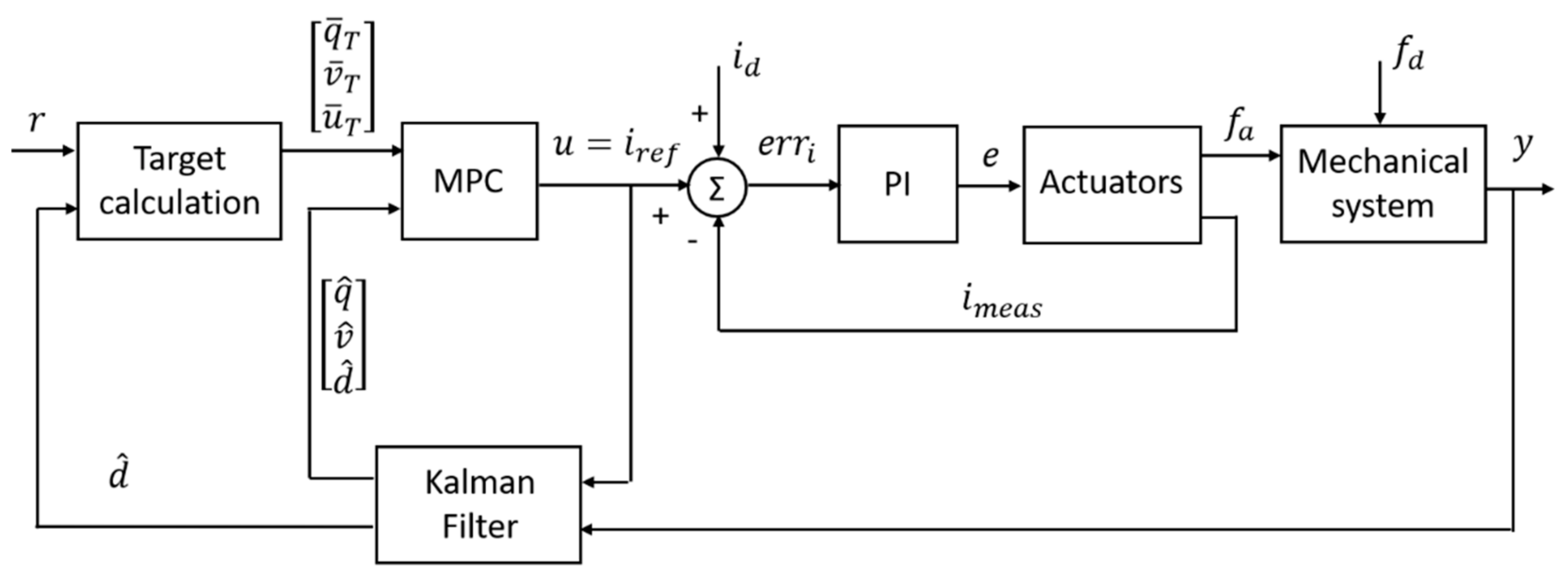
4.1. Control System Architecture

The objective of the proposed technique is to control the displacement of the moving mass to perform (a) reference tracking with the cancellation of plant-model mismatch effects; and (b) real-time estimation of low-frequency external disturbance, including load variations. The control architecture of Figure 2 is composed of an MPC block running at 5 kHz and generating the current reference $u$ for the actuators. As is usual in standard AMB systems, the current is controlled by two internal PI control loops, one per electromagnet. These inner loops run at 20 kHz. The PI integral time is selected to be equal to the time constant of the RL circuit (i.e., ${\tau }_i = {\tau }_{RL} = L_0/R$), and the proportional parameter $K_p$ is set equal to 55 V/A.

Taking the MPC current command and the displacement measured by the eddy current sensor as inputs, the Kalman filter (Equation (13)) estimates the displacement ($\widehat{q}$), velocity ($\widehat{v}$), and disturbance ($\widehat{d}$). The latter is provided to the target calculation block together with the position reference ($r$), in this case equal to 0, to obtain the state and input targets (${\overline{q}}_T,{\overline{v}}_T$, ${\overline{u}}_T$). These and the total set of Kalman filter estimates ($\widehat{q}$, $\widehat{v}$, and $\widehat{d}$.) are provided to the MPC to determine the current command $\left(u\right)$.

The control sequence repeated at each sampling time is the following: (a) the state $\widehat{x}$ and the disturbance $\widehat{d}$ are estimated by the Kalman filter; (b) the target calculation block exploits the reference $r$ and the estimated disturbance $\widehat{d}$ to generate the state and control targets sent to the MPC at the current sampling instant; and (c) the MPC solves a constrained optimization problem, based on the targets and estimations, to get a new optimal control current $u_0^{*}$, which is applied to the system during the next sampling period.

4.2. Target Calculation and MPC Problem Formulation

For offset-free tracking, at a steady state, the tracked measured output $y_{\infty }$ must reach its reference $r_{\infty }$ ($y_{\infty }$ = $r_{\infty }$).

Using the estimated disturbance $\widehat{d}\left(t\right)$ in (10), the augmented model at a steady state is expressed by

$$\left[\begin{array}{cc}A-I& B\\ C& Cd\end{array}\right]\left[\begin{array}{c}{x}_{\infty }\\ u_{\infty }\end{array}\right] = \left[\begin{array}{c}-B_d{\widehat{d}}_{\infty }\\ r_{\infty }-C_d{\widehat{d}}_{\infty }\end{array}\right]$$

(14)

This model is included in the MPC problem formulation to obtain the state and input targets. The MPC is designed considering the cost function

$$\begin{gathered} F =min{ }_{u_0} \left[{\left(x_N-{\overline{x}}_T\right)}^{\prime }P\left(x_N-{\overline{x}}_T\right)+{\displaystyle \sum }_{j=0}^{N-1}{\left(x_j-{\overline{x}}_T\right)}^{\prime }Q\left(x_j-{\overline{x}}_T\right) \\ +{\left(u_j-{\overline{u}}_T\right)}^{\prime }R\left(u_j-{\overline{u}}_T\right)\right] \end{gathered}$$

(15)

which is subject to the following constraints:

$$\begin{array}{l}{x}_{j+1} = A{x}_j+B{u}_j+B_d{d}_j, j = 0,\dots ,N,\hfill \\ x_j\in X,\hfill \\ u_j\in U, j = 0,\dots ,N-1,\hfill \\ x_N\in X_f,\hfill \\ d_{j+1} = d_j, j = 0,\dots ,N,\hfill \\ x_0 = \widehat{x}\left(0\right),\hfill \\ d_0 = \widehat{d}\left(0\right),\hfill \\ X = \left\{x_j\in {\mathbb{ℝ}}^2\right\}, j=0,\dots , N-1,\hfill \\ U = \left\{u_k\in \mathbb{ℝ}: -5 A\le u_j\le 5 A \right\}, j = 0,\dots ,N-1,\hfill \\ X_f = \left\{x_N\in {\mathbb{ℝ}}^2\right\}.\hfill \end{array}$$

(16)

where $N$ is the prediction and control horizon, and the targets ${\overline{\mathrm{x}}}_T$ and ${\overline{u}}_T$ are given by

$$\left[\begin{array}{cc}A-I& B\\ C& 0\end{array}\right]\left[\begin{array}{c}{\overline{x}}_T\\ {\overline{u}}_T\end{array}\right] = \left[\begin{array}{c}-B_d{d}_0\\ r\left(t\right)-C_d{d}_0\end{array}\right]$$

(17)

In (15), matrix $Q\succcurlyeq 0$, $R\succ 0$ and $P$ satisfies the Algebraic Riccati Equation

$$P = A^{T}PA-\left(A^{T}PB\right){\left(B^{T}PB+R\right)}^{-1}\left(B^{T}PA\right)+Q$$

(18)

A tailored solver was used for the execution of the OF-MPC controller. It was obtained by means of the $\mu AO-MPC$ code generation tool [42], which provides $C$ code libraries for the efficient online implementation of MPC problems. The solver is based on an augmented Lagrangian method together with Nesterov’s gradient method and guarantees a deterministic execution time [42], since the maximum computation time required by the MPC in the dSpace hardware is about 25 $\mathsf{\mu }\mathrm{s}$. At each sampling instant $k$, the constrained optimal control problem (15)–(17) is solved over a finite time prediction horizon $N$, using the current observed state of the plant $\widehat{x}\left(k\right)$. The method yields an optimal control sequence $U_0\left(k\right) = \left\{{\mathrm{u}}_0^{*}, \dots ,{\mathrm{u}}_{N-1}^{*}\right\}$, of which only the first command $u\left(k\right) = u_0^{*}$ is applied to the plant.

The MPC design parameters adopted in the present case are listed in

Table 3. OF-MPC design parameters.

Parameter	Value
$N$	12
$Q$	$\left[\begin{array}{cc}5\times {10}^6& 0\\ 0& 0.1\end{array}\right]$
$R$	1
$P$	$\left[\begin{array}{cc}98255756& 804198\\ 804198& 10020\end{array}\right]$

. The prediction horizon $N$ is selected as the smallest value to obtain a fast-enough response, but guaranteeing the feasibility of the constrained optimal control problem formulation. As is common practice, the value of $R$ is fixed to 1, while $Q$, i.e., the weight matrix for the state $q\left(t\right)$ and $v\left(t\right)$, is designed to obtain a reasonable compromise between a sufficiently fast response and low noise amplification. The matrix $P$ is obtained from (18).

A nonlinear version of the proposed method could be investigated to take into account the plant nonlinearity effects [36]. In this case, the design should be conducted considering Equation (2) instead of Equation (3). The technique would be based on a different solver and on the replacement of the Kalman filter with a nonlinear observer method. The designer should take care of possible issues related to the convergence of the solution and guarantee a deterministic execution time [36].

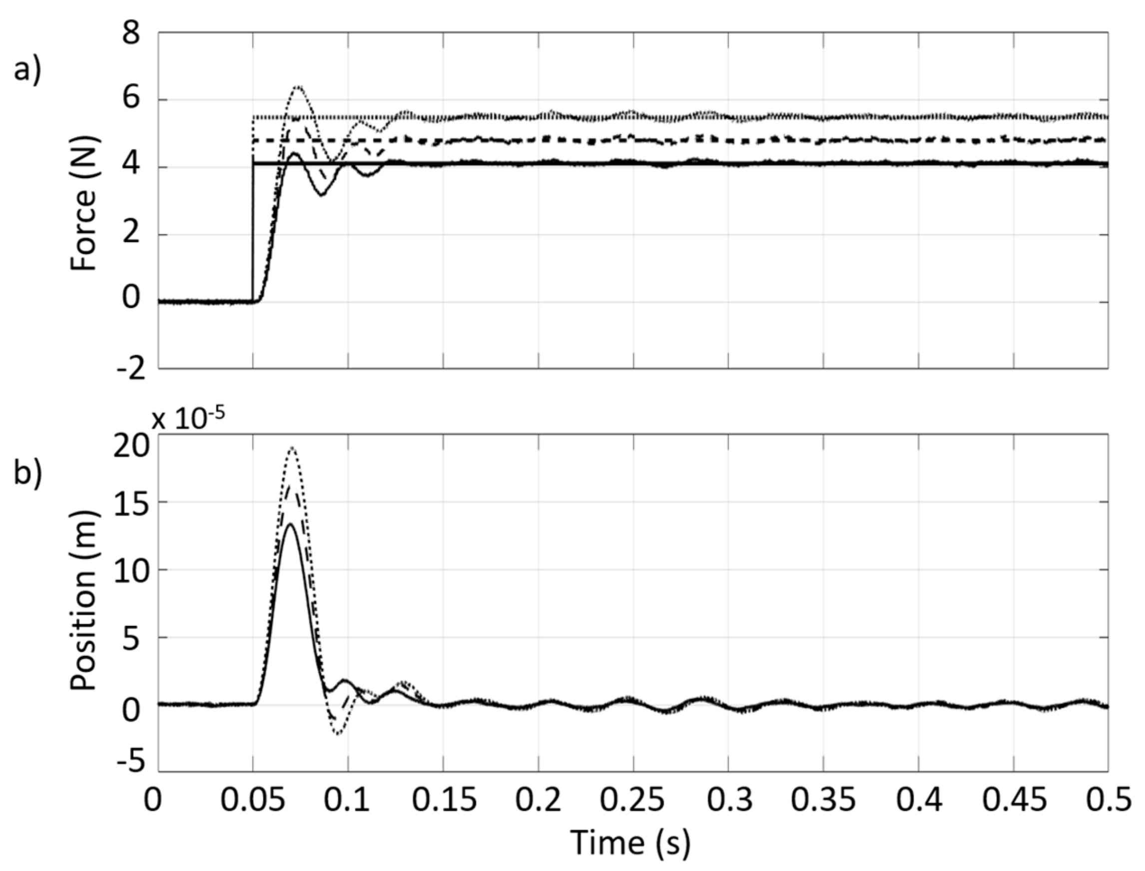
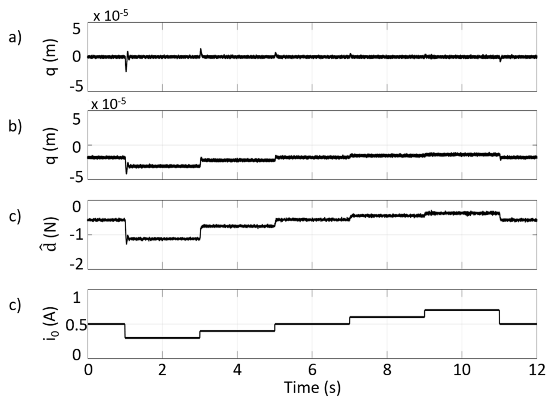
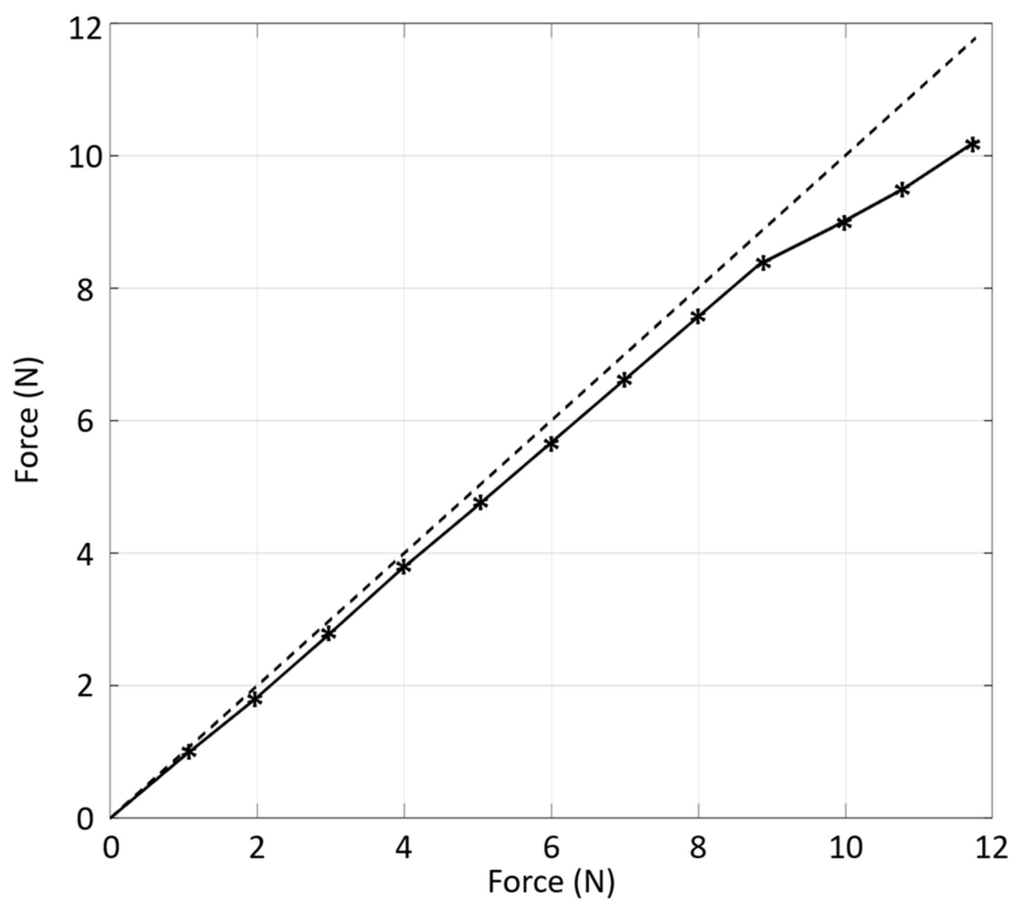
5. Experimental Results and Discussion

The experimental tests are conducted to validate the system performance in terms of: correctness of the Kalman filter estimation, offset-tracking with the cancellation of plant-model mismatch, and low-frequency disturbance estimation. The tests are performed with the arm of the AMB system in a vertical direction to avoid the load due to its weight and with a bias current of 0.5 A.

The first test consists of providing a step excitation through the actuators with a disturbance current ($i_d$ in Figure 2) of 0.2 A, corresponding to a force of about 3.5 N at a nominal airgap. The obtained results are reported in Figure 3. In particular, Figure 3a illustrates the nominal force provided to the system (dotted line), the force obtained from (2) (dashed line), and its estimate from the Kalman filter (solid line). It can be pointed out that, even with no current disturbance (t < 0.1 s), the control output and disturbance estimation values are nonzero, which is caused by the plant-model mismatch. As expected from (6), both effects of plant-model mismatch and external disturbances are lumped into a force estimate to move the controller targets and guarantee offset-free tracking. Figure 3b illustrates the simulated (dashed line) and experimental (solid line) MPC command: providing the disturbance current $i_d$, the Kalman filter estimates change, and the controller target is modified to achieve zero offset on the output. Finally, Figure 3c reports the comparison between the measured position (solid line) and that estimated from the Kalman filter (dashed line) (the simulation results are not reported in this plot for clarity’s sake). The proposed controller is able to recover the effect of the disturbance and reach a null offset in about 0.06 s. The same figure evidences that since the position estimation has low noise (RMS measured in 1 s = 0.79 $\mathsf{\mu }\mathrm{m}$) with respect to the measurement (RMS measured in 1 s = 1.12 $\mathsf{\mu }\mathrm{m}$), the signals in the control loop result are inherently filtered and clean. The good match between the simulation and experimental results demonstrates the effectiveness of the modeling approach.

The same test is conducted with different amplitudes of excitation to obtain a more exhaustive validation in different operating conditions. Figure 4a shows the comparison between the nominal and the estimated disturbance force, and Figure 4b displays the corresponding displacement. In this case, the offset due to the plant-model mismatch is removed in post-processing to highlight the correctness of the external disturbance force estimation.

It can be noted that, while the transient response changes considerably because of the nonlinear nature of the plant, at a steady state, the force estimate is still consistent with the current disturbance. This is due to the well-known physical linearization of AMB actuators’ characteristics (see (2)) taking place when the moving mass is in a centered position ($q = 0$), and both electromagnets are active, ($i_c < i_0$). In these conditions, the current-force characteristic is substantially linear and coefficient $k_i$ does not depend on the new control current value, provided that the moving mass reaches the offset free displacement at the center of the gap.

The next set of tests is performed to evaluate the capability of the proposed method to cancel the plant-model mismatch. As mentioned above, the linear model has been obtained considering a bias current of 0.5 A. If a different value of bias current is set in the experimental tests, the model is not representative of the plant anymore. This plant-model mismatch clearly affects the behaviour of simple MPC architectures when no integral action exists, while the proposed OF-MPC method allows this issue to be overcome and, at the same time, the amount of disturbance to be evaluated.

Figure 5 illustrates the results of the tests performed by imposing consecutive changes of the bias current from 0.3 A to 0.7 A (d) and comparing the behavior of the displacement of the proposed OF-MPC (a) and of a simple MPC (b) which is based on the same formulation but with targets to the origin (i.e., ${\overline{x}}_t = {\overline{u}}_t = 0$, which means no knowledge about plant-model mismatch and disturbance forces). As stated before, both controllers have been designed on the base of a plant model that considers a bias current of 0.5 A. The displacement plot of Figure 5a shows that the OF-MPC compensates for the plant-model mismatch very effectively, providing, at the same time, an estimation of the disturbance force (c). However, from Figure 5b, an offset in the displacement is always present with the MPC controller, even when bias current is the designed one.

The aim of the last set of tests is to evaluate the correctness of the load variation estimation. The tests are performed as illustrated in Figure 6 by applying known values of force to the system by means of direct weights $\left(L\right)$ acting on the arm by means of a pulley and a piece of string.

Figure 7 shows the estimation performance comparing the estimated force (solid line) with the applied force (dashed line). The precision of the estimation is around 97% until the control current is lower than the bias current (0.5 A) and decreases down to 90% when one electromagnet is switched off. It is worth noticing that if the disturbance requires switching off one electromagnet (the control current is higher than the bias current), the system is not working in linear differential mode anymore and the electromagnets work in a nonlinear range, even in the nominal position. The force estimation is still acceptable even under these conditions, and this shows the good performance of the proposed strategy, even in a nonlinear operating range.

6. Conclusions

In this paper, the application of linear Offset-Free Model Predictive Control (OF-MPC) to a single-axis active magnetic bearing system has been presented. The proposed method is based on a disturbance observer with an augmented plant model including an input disturbance estimation. The proposed technique allows the well-known advantages of MPC to be exploited and, at the same time, the effect of plant-model mismatch in the reference tracking to be overcome. This architecture allows the real-time estimation of the low-frequency disturbance applied to the system. This last property is of great interest in industrial applications like compressors and blowers, where keeping the reference position is critical to insuring the system functionality, even when the axial load changes according to the operating conditions. The modeling and control design have been described and validated experimentally for a single-axis AMB system with a set of tests that demonstrate the effectiveness of the approach in terms of reference tracking with the cancellation of plant-model mismatch effects and estimation of low-frequency disturbances and load variations.

References

1. Bleuler, H.; Cole, M.; Keogh, P.; Larsonneur, R.; Maslen, E.; Nordmann, R.; Okada, Y.; Schweitz, G.; Traxler, A. Magnetic Bearings: Theory, Design, and Application to Rotating Machinery; Springer Science & Business Media: Berlin/Heidelberg, Germany, 2009. [Google Scholar]
2. Chiba, A.; Fukao, T.; Ichikawa, O.; Oshima, M.; Takemoto, M.; Dorrell, D.G. Magnetic Bearings and Bearingless Drives; Elsevier: Amsterdam, The Netherlands, 2005. [Google Scholar]
3. Song, X.; Throckmorton, A.L.; Untaroiu, A.; Patel, S.; Allaire, P.E.; Wood, H.G.; Olsen, D.B. Axial flow blood pumps. ASAIO J. 2003, 49, 355–364. [Google Scholar] [PubMed]
4. Filatov, A.; Hawkins, L.; McMullen, P. Homopolar Permanent-Magnet-Biased Actuators and Their Application in Rotational Active Magnetic Bearing Systems. Actuators 2016, 5, 26. [Google Scholar] [CrossRef]
5. Chen, S.-L.; Weng, C.-C. Robust control of a voltage-controlled three-pole active magnetic bearing system. IEEE/ASME Trans. Mechatron. 2010, 15, 381–388. [Google Scholar] [CrossRef]
6. Darbandi, S.M.; Behzad, M.; Salarieh, H.; Mehdigholi, H. Linear output feedback control of a three-pole magnetic bearing. IEEE/ASME Trans. Mechatron. 2014, 19, 1323–1330. [Google Scholar]
7. Noh, M.D.; Maslen, E.H. Self-sensing magnetic bearings using parameter estimation. IEEE Trans. Instrum. Meas. 1997, 46, 45–50. [Google Scholar] [CrossRef] [Green Version]
8. Mizuno, T.; Bleuler, H. Self-sensing magnetic bearing control system design using the geometric approach. Control Eng. Pract. 1995, 3, 925–932. [Google Scholar] [CrossRef]
9. Bonfitto, A.; Tonoli, A.; Silvagni, M. Sensorless active magnetic dampers for the control of rotors. Mechatronics 2017, 47, 195–207. [Google Scholar] [CrossRef]
10. Lei, S.; Palazzolo, A. Control of flexible rotor systems with active magnetic bearings. J. Sound Vib. 2008, 314, 19–38. [Google Scholar] [CrossRef]
11. Ren, Z.; Stephens, L.S. Closed-loop performance of a six degree-of-freedom precision magnetic actuator. IEEE/ASME Trans. Mechatron. 2005, 10, 666–674. [Google Scholar] [CrossRef]
12. Grabner, H.; Silber, S.; Amrhein, W. Bearingless torque motor-modeling and control. In Proceedings of the 13th International Symposium on Magnetic Bearings (ISMB), Arlington, VA, USA, 6–9 August 2012. [Google Scholar]
13. Silber, S.; Grabner, H.; Lohninger, R.; Amrhein, W. Design aspects of bearingless torque motors. In Proceedings of the 13th International Symposium on Magnetic Bearings (ISMB), Arlington, VA, USA, 6–9 August 2012. [Google Scholar]
14. Maslen, E.; Montie, D. Sliding mode control of magnetic bearings: A hardware perspective. J. Eng. Gas Turbines Power 2001, 123, 878–885. [Google Scholar] [CrossRef]
15. Sivrioglu, S.; Nonami, K. Sliding mode control with time-varying hyperplane for AMB systems. IEEE/ASME Trans. Mechatron. 1998, 3, 51–59. [Google Scholar] [CrossRef]
16. Nonami, K.; He, W.; Nishimura, H. Robust control of magnetic levitation systems by means of H control/μ-synthesis. JSME Int. J. Ser. C Dyn. Control Robot. Des. Manuf. 1994, 37, 513–520. [Google Scholar] [CrossRef]
17. Hac, A.; Tomizuka, M. Application of learning control to active damping of forced vibration for periodically time variant systems. J. Vib. Acoust. 1990, 112, 489–496. [Google Scholar] [CrossRef]
18. Betschon, F.; Knospe, C.R. Reducing magnetic bearing currents via gain scheduled adaptive control. IEEE/ASME Trans. Mechatron. 2001, 6, 437–443. [Google Scholar] [CrossRef]
19. Ulbig, A.; Olaru, S.; Dumur, D.; Boucher, P. Explicit nonlinear predictive control for a magnetic levitation system. Asian J. Control 2010, 12, 434–442. [Google Scholar] [CrossRef]
20. Fama, R.C.; Lopes, R.V.; Milhan, A.; Galvão, R.; Lastra, B. Predictive control of a magnetic levitation system with explicit treatment of operational constraints. In Proceedings of the 18th International Congress of Mechanical Engineering, Ouro Preto, Brazil, 6–11 November 2005. [Google Scholar]
21. Cavalca, M.S.M.; Galvão, R.K.H.; Yoneyama, T. Robust model predictive control for a magnetic levitation system employing linear matrix inequalities. ABCM Symp. Ser. Mechatron. 2010, 4, 147–155. [Google Scholar]
22. Bächle, T.; Hentzelt, S.; Graichen, K. Nonlinear model predictive control of a magnetic levitation system. Control Eng. Pract. 2013, 21, 1250–1258. [Google Scholar] [CrossRef]
23. Klaučo, M.; Kalúz, M.; Kvasnica, M. Real-time implementation of an explicit MPC-based reference governor for control of a magnetic levitation system. Control Eng. Pract. 2017, 60, 99–105. [Google Scholar] [CrossRef]
24. Tsao, J.-G.; Sheu, L.-T.; Yang, L.-F. Adaptive synchronization control of the magnetically suspended rotor system. Dyn. Control 2000, 10, 239–253. [Google Scholar] [CrossRef]
25. Zhang, C.; Tseng, K.J.; Xiao, Y.; Zhu, K.Y. Model-based predictive control for a compact and efficient flywheel energy storage system with magnetically assisted bearings. In Proceedings of the 2004 IEEE 35th Annual Power Electronics Specialists Conference (IEEE Cat. No.04CH37551), Aachen, Germany, 20–25 June 2004; Volume 5, pp. 3573–3579. [Google Scholar]
26. Chowdhury, A.; Sarjaš, A. Finite Element Modelling of a Field-Sensed Magnetic Suspended System for Accurate Proximity Measurement Based on a Sensor Fusion Algorithm with Unscented Kalman Filter. Sensors 2016, 16, 1504. [Google Scholar] [CrossRef] [PubMed]
27. Castellanos, L.M.; Bonfitto, A.; Tonoli, A.; Amati, N. Identification of Force-Displacement and Force-Current Factors in an Active Magnetic Bearing System. In Proceedings of the 18th Annual IEEE International Conference on Electro Information Technology, Rochester, MI, USA, 3–5 May 2018. [Google Scholar]
28. Afonso, R.J.M.; Galvão, R.K.H. Predictive control of a magnetic levitation system with infeasibility handling by relaxation of output constraints. ABCM Symp. Ser. Mechatron. 2007, 3, 11–18. [Google Scholar]
29. Pannocchia, G.; Rawlings, J.B. Disturbance models for offset-free model-predictive control. AIChE J. 2003, 49, 426–437. [Google Scholar] [CrossRef]
30. Rawlings, J.B. Tutorial overview of model predictive control. IEEE Control Syst. 2000, 20, 38–52. [Google Scholar] [Green Version]
31. Wang, X.; Ding, B.; Yang, X.; Ye, Z. Design and Application of Offset-Free Model Predictive Control Disturbance Observation Method. J. Control Sci. Eng. 2016, 2016, 7279430. [Google Scholar] [CrossRef]
32. Maeder, U.; Borrelli, F.; Morari, M. Linear offset-free model predictive control. Automatica 2009, 45, 2214–2222. [Google Scholar] [CrossRef]
33. Pannocchia, G. Offset-free tracking MPC: A tutorial review and comparison of different formulations. In Proceedings of the 2015 European Control Conference (ECC), Linz, Austria, 15–17 July 2015; pp. 527–532. [Google Scholar]
34. Borrelli, F.; Morari, M. Offset free model predictive control. In Proceedings of the 2007 46th IEEE Conference on Decision and Control, New Orleans, LA, USA, 12–14 December 2007; pp. 1245–1250. [Google Scholar]
35. Muske, K.R.; Badgwell, T.A. Disturbance modeling for offset-free linear model predictive control. J. Process Control 2002, 12, 617–632. [Google Scholar] [CrossRef]
36. Morari, M.; Maeder, U. Nonlinear offset-free model predictive control. Automatica 2012, 48, 2059–2067. [Google Scholar] [CrossRef]
37. Kim, S.-K.; Choi, D.-K.; Lee, K.-B.; Lee, Y.I. Offset-free model predictive control for the power control of three-phase AC/DC converters. IEEE Trans. Ind. Electron. 2015, 62, 7114–7126. [Google Scholar] [CrossRef]
38. Bender, F.A.; Göltz, S.; Bräunl, T.; Sawodny, O. Modeling and Offset-Free Model Predictive Control of a Hydraulic Mini Excavator. IEEE Trans. Autom. Sci. Eng. 2017, 14, 1682–1694. [Google Scholar] [CrossRef]
39. Askaria, M.; Moghavvemi, M.; Almurib, H.A.F.; Muttaqi, K.M. An offset-free multivariable model predictive control for quadruple tanks system. In Proceedings of the 2014 IEEE Industry Applications Society Annual Meeting, Vancouver, BC, Canada, 5–9 October 2014; pp. 1–8. [Google Scholar]
40. Pannocchia, G.; Laachi, N.; Rawlings, J.B. A candidate to replace PID control: SISO-constrained LQ control. AIChE J. 2005, 51, 1178–1189. [Google Scholar] [CrossRef]
41. Skogestad, S.; Postlewhite, I. Multivariable Feedback Control: Analysis and Design; Wiley: New York, NY, USA, 2001. [Google Scholar]
42. Zometa, P.; Kögel, M.; Findeisen, R. μAO-MPC: A free code generation tool for embedded real-time linear model predictive control. In Proceedings of the 2013 American Control Conference (ACC), Washington, DC, USA, 17–19 June 2013; pp. 5320–5325. [Google Scholar]
Figure 1. Single-degree-of-freedom AMB system. (a) Picture of the test rig. (b) System layout: (1) Pivot; (2) Displacement sensor; (3) Moving mass; (4) Electromagnet.
Actuators 07 00046 g001
Figure 2. Control system architecture.
Actuators 07 00046 g002
Figure 3. Step excitation through the actuators with a current i d   =   0.25   A . (a) Nominal force applied to the system (dotted line); force from model simulation (dashed line); force estimated experimentally by the Kalman filter (solid line). (b) MPC command (dashed line: simulation result; solid line: experimental result). (c) Displacement of the mass (solid line: eddy current sensor direct measurement; dashed line: Kalman filter estimation).
Actuators 07 00046 g003
Figure 4. Step excitation at different force amplitudes ( i d   = 0.3   A ,   0.35   A ,   0.4   A ). (a) Nominal vs. estimated applied force. (b) Displacement of the mass.
Actuators 07 00046 g004
Figure 5. Effects of the plant-model mismatch on OF-MPC (a) and MPC (b) architectures. (c) is the estimation of the force equivalent to the plant-model mismatch (obtained only with OF-MPC architecture) and (d) is the variation of bias current provided to the plant.
Actuators 07 00046 g005
Figure 6. Experimental setup for the load variation estimation test. Picture (a) and layout (b) of the setup. L : variable load.
Actuators 07 00046 g006
Figure 7. Load variation estimation test. Dashed line: real applied force. Solid line: estimated force.
Actuators 07 00046 g007