Morphology-Guided Nonlinear Structural Evaluation of a Hybrid Bio-Inspired Soft Robotic Actuator

Abstract

Soft robotic actuators exploit structural compliance to produce adaptive motion, but their response depends strongly on the interaction between geometry, material distribution, specific reinforcement, and actuation. This manuscript presents a bio-inspired hybrid soft actuator based on the elongated, continuously deformable morphology of the arrow worm and evaluates whether its bending response can be programmed through structural morphology. Four force-controlled nonlinear static finite element studies were performed in SOLIDWORKS Simulation using a hyperelastic Ogden model for the Ecoflex^TM 00-50 body and orthotropic models for the Thermoplastic Polyurethane (TPU) 68D reinforcement spine and Acrylonitrile styrene acrylate (ASA) pressure pad. Across the analysed force activation levels, maximum resultant displacement increased from 0.948 mm to 17.88 mm, equivalent strain from 0.005268 to 0.06833, and maximum von Mises stress from 0.596 MPa to 5.447 MPa. Simultaneously, effective-average incremental stiffness decreased from 0.21097 N/mm to 0.04846 N/mm, corresponding to a 77.03% reduction. These findings demonstrate progressive nonlinear softening and the transformation of mechanical input into a guided global shape change. A representative comparison with existing measurements of the fabricated actuator was additionally used to quantitatively cross-check the predicted bending response. The result of the morphological calculation was also the creation of a morphological map for quantitative and qualitative assessment of normalized morphological descriptors of the actuator.

1. Introduction

The development of soft robotic fingers appears to be driven by the need for grippers that can safely interact with fragile, irregular or unknown objects. Unlike rigid mechanisms, soft structures seem to use compliance as a functional design feature where deformation enables passive adaptation, distributed contact and safer manipulation [1,2,3]. Some researchers argue this principle can be strongly inspired by biological systems, where motion is generated through the interaction of muscles, tendons, ligaments, and compliant tissues rather than through rigid joints alone. Researchers often suggest such morphological structures can reduce local contact stresses, improve shape conformity, and simplify grasping tasks in which the object geometry or stiffness is not precisely known in advance—important, though not always achievable under all conditions.

Viewed from this perspective, compliance is not merely a passive consequence of using soft materials but can be deliberately incorporated into the mechanical architecture as a functional design parameter. This principle is closely related to morphological computation and embodied or physical intelligence, according to which part of the functionality conventionally assigned to sensing and control can be supported by the geometry, material properties, compliance and mechanical interaction of the robotic body with its environment [4,5,6]. For soft robotic fingers, this implies that the desired deformation does not necessarily have to be generated or corrected exclusively by the actuator and controller; instead, the structure itself can mechanically favour selected deformation modes while suppressing undesirable ones.

This concept has been extensively demonstrated in mechanically programmed soft actuators. Fiber-reinforced elastomeric actuators use the orientation and arrangement of reinforcing fibers to introduce anisotropic constraints, thereby converting a relatively simple actuation input into predefined extension, contraction, bending, or twisting responses [7,8]. Similarly, multimaterial and bio-inspired architectures can encode deformation through local differences in geometry, reinforcement, and material properties [9]. These approaches illustrate the broader principle of programmed compliance and stiffness-distribution design, in which functional performance is determined not only by the overall softness of the structure but by where compliance and stiffness are located within it. This distinction is particularly important in soft grippers because excessive or uniformly distributed compliance can compromise force transmission, load-bearing capability, deformation stability, and repeatability, motivating the development of structural reinforcement and stiffness-control strategies [10,11].

Despite these advances, much of the established work on mechanical programming has focused on fiber-reinforced fluidic actuators, multimaterial actuator bodies, or mechanisms capable of actively changing their stiffness. Comparatively less attention has been devoted to hybrid soft-finger architectures in which deformation is pre-programmed by a passive, geometrically defined internal structure that is mechanically distinct from both the surrounding compliant body and the actuation element. In particular, the relationship between such an internal structure, the resulting distribution of structural stiffness, and the preferred deformation path requires further numerical investigation when the objective is to obtain predictable bending without introducing additional rigid joints or complex transmission mechanisms. This constitutes the specific research gap addressed in the present study.

The proposed design approaches this problem through a compliant internal 3D-printed TPU spine embedded within a softer finger body. Rather than treating the spine only as reinforcement, its geometry and position are intended to act as a passive morphological programming element that establishes the preferred bending plane, redistributes structural stiffness, supports force transmission, and constrains undesired deformation. The novelty therefore lies not in the general concepts of morphological computation, compliance programming, or structural reinforcement themselves, but in their implementation and numerical assessment within this specific hybrid finger architecture. The finite element analyses are used to determine whether the mechanically programmed internal morphology can produce the intended deformation modes and acceptable stress and strain distributions under separately defined actuation loading conditions.

Within this mechanically programmed architecture, the integration of a compact actuator remains a second important design consideration. Pneumatic actuators can produce large deformation and natural compliance, but they need several additional components such as pumps, valves, tubing, and pressure control parts.

Within this mechanically programmed architecture, the integration of a compact actuator remains a second important design consideration. Electric motors provide precise control and quick response, though they often require transmissions, tendons, gears, or linkages to achieve distributed bending in a soft finger. Shape memory alloys (SMAs), particularly NiTi-based alloys, present another approach, as they generate mechanical work directly through thermally induced phase transformation while staying compact, lightweight, and quiet [12,13,14,15,16,17]. These characteristics make SMA actuators suitable for small robotic grippers, prosthetic fingers, rehabilitation devices, and biomimetic hands [18,19,20,21]. Their high specific work and straightforward electrical activation are especially valuable in cases where the actuator must be built directly into a compact end-effector. SMA actuators have been used in various forms, including wires, wire bundles, springs, tendons, torsional hinges and embedded composite elements [22,23,24,25]. SMA springs offer a greater stroke within a compact volume, which benefits soft fingers and grippers. However, their lower force output, cooling rate, and fatigue performance must be taken into account during design [26,27,28,29,30]. There have been several studies demonstrating SMA-driven soft robotic hands, curved soft actuators, reversible composite actuators, compact parallel grippers, and two-finger automation grippers [19,31,32,33,34]. However, SMA-based soft fingers still face notable limitations. Their motion depends on nonlinear thermo-mechanical behavior, hysteresis, and strong coupling between electrical input, temperature, stress, and deformation [35,36,37,38]. The heating phase can be sped up by Joule heating, yet the cooling phase often restricts the total cycle time and actuation frequency [39,40,41]. This issue becomes even more significant when the SMA element is embedded in an elastomeric or composite body, where heat transfer, local strain concentration, friction, and interface effects all affect the final deformation. If the active element is too tightly constrained by the surrounding soft material, part of the generated stroke may be lost through internal deformation, local stress buildup, or frictional dissipation. Thus, the mechanical and thermal integration of the SMA element within the soft body is just as important as the actuator material itself.

For this reason, finite element analysis serves as a useful tool in designing SMA-actuated soft fingers. Numerical evaluation of morphological programming provides a complementary means of assessing bending behavior and stress and strain localization alongside experimental testing, particularly when detailed internal mechanical yields cannot be obtained directly from the fabricated actuator [38,42]. This approach is particularly helpful for hybrid soft structures, where an elastomeric body ensures compliance while an internal reinforcement or spine directs the preferred bending mode. The design logic resembles that of biological fingers, where the structure is not entirely soft but mechanically arranged to produce stable, repeatable, and functional deformation. In this way, the spine not only strengthens the finger but also functions as a design element that shapes the deformation path, bending plane, and recovery behavior. The proposed architecture combines a soft compliant body, an internal 3D printed TPU spine, a pressure pad for attachment and transmission of tensile force, and cavities containing antagonistically arranged SMA contraction springs. Because the actuator cavities remain unfilled, the contraction elements can operate with reduced direct mechanical constraint from the surrounding elastomer, which is intended to limit parasitic deformation and improve transmission of the generated displacement. The main role of actuator stiffness will be carried by the TPU spine, which is expected to guide the bending direction and improve shape stability. The analysis will include separate nonlinear static numerical studies in which individual force working modes will be examined.

The purpose of these analyses is to numerically evaluate the mechanically programmed deformation of the proposed hybrid soft finger, with particular emphasis on the influence of the internal TPU spine and selected material properties on the preferred bending behavior, stress and strain distribution, and overall structural response. To establish a direct link between the numerical predictions and the physical actuator, a representative numerical state is additionally compared with previously acquired optical measurements from a fabricated P5 prototype with the same nominal 2.0 mm reinforcement thickness. The comparison focuses on the global bending response and deformed shape and is intended as a structural experimental cross-check rather than as a validation of the complete electro-thermo-mechanical behavior of the SMA actuator.

Accordingly, the contribution of this work is threefold. First, a hybrid Ecoflex–TPU–ASA soft-finger architecture is evaluated in which the internal TPU spine is treated as a prescribed passive stiffness-distribution element rather than solely as reinforcement. Second, an experimentally informed force-controlled nonlinear finite element model is used to characterize the load-dependent structural response and to identify the preferred deformation mode and associated stress–strain fields. Third, a design-level descriptor framework and a representative experimental cross-check are used to distinguish morphology-dependent deformation trends from the quantitative limitations of the simplified equivalent-force SMA representation. The study does not perform topology optimization and does not constitute a coupled thermo-mechanical SMA model.

2. Materials and Methods

2.1. Bio-Inspiration in Actuator Design

Nature offers many examples of efficient, adaptable, and mechanically robust solutions that have evolved to perform complex tasks with minimal structural complexity. In soft robotics, biological organisms often serve as sources of inspiration since their bodies can produce flexible motion, safe interaction with the environment, and shape adaptation without depending on rigid joints or conventional mechanical systems.

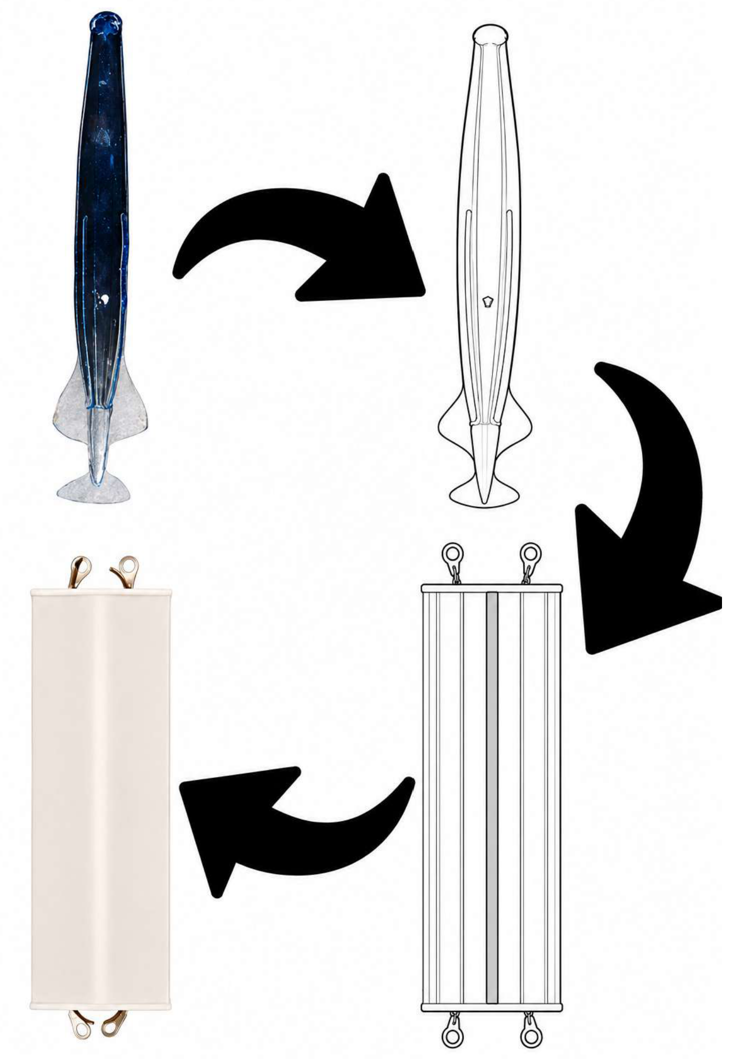
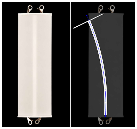
The bio-inspired design concept of the proposed silicone finger was based on the morphology and locomotion principle of the arrow worm, a marine invertebrate belonging to the phylum Chaetognatha. As shown in the Figure 1, the biological model has an elongated, rounded, and continuously deformable body structure that allows significant reversible bending without rigid articulated joints. Despite its soft-body form, the arrow worm contains internal supporting and reinforcing elements that provide directional stability and controlled body deformation during motion. This biological configuration is closely mirrored in the proposed silicone finger, where a compliant silicone body is mechanically supported by an internal guiding structure that defines and stabilizes the preferred bending pattern.

Unlike conventional mechanisms composed of discrete skeletal segments and localized rotational axes, the arrow worm’s movement occurs through distributed deformation of its entire soft body. This biomechanical principle directly aligns with the functional concept of the developed silicone finger, where bending arises not from revolute joints but from controlled deformation of a reinforced compliant structure. Therefore, the arrow worm serves as a fitting biological analogy for the proposed soft robotic finger.

2.2. Conceptual and Mechanical Design

In soft robotics, mechanical deformation programming is one of the basic design principles, in which the desired motion behavior of the effector is not created exclusively by a control algorithm but is partially encoded directly in its material-geometric structure. In combination with the biomimetic approach outlined in Section 2.1, the resulting motion trajectory is determined by the shape and arrangement of cavities, local expansion constraints, material layering, and reinforcement elements that introduce spatially inhomogeneous and directionally dependent compliance. Although actuation can be implemented by various principles, for example, pneumatically, hydraulically, thermally, or through smart materials, the interaction between the elastomer matrix and the design constraints has a decisive influence on the resulting deformation mode. This interaction determines whether the effector will perform dominant bending, torsion, axial extension, or a combined spatial motion.

Based on the principle of mechanical deformation programming, the conceptual design of the soft actuator considers a material-geometric structure in which the resulting movement is determined not only by the active element itself but also by the spatial distribution of stiffness and compliance within the finger body. For this reason, the design focuses on silicone elastomers that make it possible to create flexible structures capable of large elastic deformations, safe contact with objects, and consistent return to the starting position. Particular attention should be given to the regions around cavities, reinforcements, and thickness transitions, where stress concentration and damage initiation can occur. When integrating the SMA element, it is therefore necessary to consider not only the mechanical compatibility of the elastomer with the metal actuator but also the effect of cyclic heating on the stability of the material and the interface between individual structural parts. However, thermal analysis is not part of this manuscript.

The proposed architecture follows the concept in which the contraction of the SMA spring acts directly within the body of the soft finger. The elastomer structure’s role is not only to passively transmit the actuator’s effect but also to transform its contraction into the desired bending motion. The functional behavior of the finger is thus determined by the combination of the SMA spring’s position, the geometry of the cavities, the thickness of the elastomer wall, and any reinforcement components.

The flexible structure designed in this way can also reduce sensitivity to positional inaccuracies, enlarge the contact area during gripping, and lower the risk of damage to the manipulated object. The key design task is to mechanically program the bend so that the deformation upon activation of the SMA spring is repeatable, energy-efficient, and suitable for generating gripping force. Equally important is the finger’s ability to reliably return to its original position after deactivation of the SMA element, since this return movement is mainly ensured by the elastic response of the elastomer matrix. The design must therefore balance the need for sufficient compliance to allow large deformation with the requirement for adequate return stiffness and shape stability.

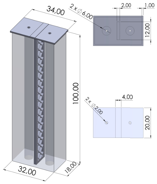
The final P5 architecture was selected on the basis of the iterative development and experimental assessment of preceding soft-finger variants documented by Romancik work [43]. The development sequence showed that the combination of a monolithic silicone elastomer body Ecoflex^TM 00-50 (Smooth-On, Inc., Macungie, PA, USA), longitudinal cavities allowing unconstrained SMA-spring contraction, and a mechanically anchored TPU reinforcement provided the most suitable basis for repeatable guided bending and elastic return. The current study therefore focuses on the nonlinear structural evaluation of this final P5 architecture, as shown in Figure 2. The basic design parameters of the configuration used in the numerical model are shown in Figure 3.

The soft finger consists of a monolithic body made of Ecoflex^TM 00-50, within which a reinforcement of Bambu TPU for AMS (Shore hardness 68D; Shenzhen Tuozhu Technology Co., Ltd. [Bambu Lab], Shenzhen, Guangdong, China) next Bambu TPU 68D featuring a lattice topology and a thickness of 2 mm is integrated. This design strengthens the mechanical bond with the elastomer and lowers the risk of slippage or delamination during cyclic loading. At the same time, it helps stabilize the bending motion and supports the return to the initial position. In short, the reinforcement increases the bending stiffness of the structure. Another important feature is the longitudinal symmetrical cavities formed in the mold using inserts, where the SMA springs can freely contract during actuation and thus operate antagonistically without being directly cast into the silicone. From the conceptual tests, it was observed that direct casting of the springs into the elastomer leads to unwanted internal deformations of the structure and, consequently, rapid degradation of the entire component. Moreover, this configuration reduces friction and local shear stress on the Ecoflex while improving the repeatability of actuation.

2.2.1. SMA Spring Representation and Model Scope

The fabricated P5 actuator uses a contraction-type NiTi spring with a free length $L_0=140$ mm, coil diameter $D=7$ mm, and wire diameter $d=0.75$ mm. Previous experimental characterization yielded a maximum axial contraction of approximately $\Delta L_{\max }=29$ mm at $I=3$ A, corresponding to a nominal free-spring contraction of approximately 20.7% [43]. The spring operates inside an unfilled longitudinal cavity, where its contraction is transferred to the soft structure through the mechanical attachment and pressure-pad region.

$${\epsilon }_{\mathrm{SMA},\max }={\displaystyle \frac{\Delta L_{\max }}{L_0}}={\displaystyle \frac{29}{140}}\approx 0.207.$$

(1)

The force–stroke response of an SMA spring is not represented by a single constant stiffness because it depends on temperature, phase transformation, loading history, hysteresis, and operating stroke [22,35,37]. In the present finite element study, the NiTi spring is therefore not constitutively modeled as a thermo-mechanical body. Its action is represented only by an equivalent quasi-static tensile force applied at the attachment region. Temperature-dependent stiffness, hysteresis, stroke-dependent force generation, Joule heating, cooling behavior, and local attachment effects such as slip or friction are not solved explicitly. Consequently, the numerical model should be interpreted as a nonlinear structural-response model of the Ecoflex–TPU–ASA assembly rather than as a fully coupled thermo-mechanical model of the SMA actuator.

2.2.2. Existing Experimental Reference Configuration

The experimental reference used in the present study was obtained from the previously fabricated P5 soft-finger prototype documented by Romancik [43]. The P5 concept uses a monolithic Ecoflex body, a centrally positioned Bambu TPU 68D lattice reinforcement, and longitudinal cavities allowing the NiTi contraction springs to operate without being directly embedded in the elastomer. Four reinforcement thicknesses were experimentally investigated in the original test campaign. For the present comparison, only the $t=2.0$ mm configuration was selected because this thickness corresponds to the reinforcement geometry adopted in the finite element model investigated in this manuscript.

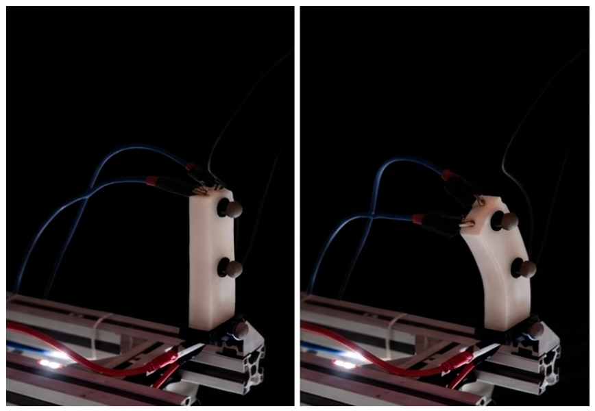
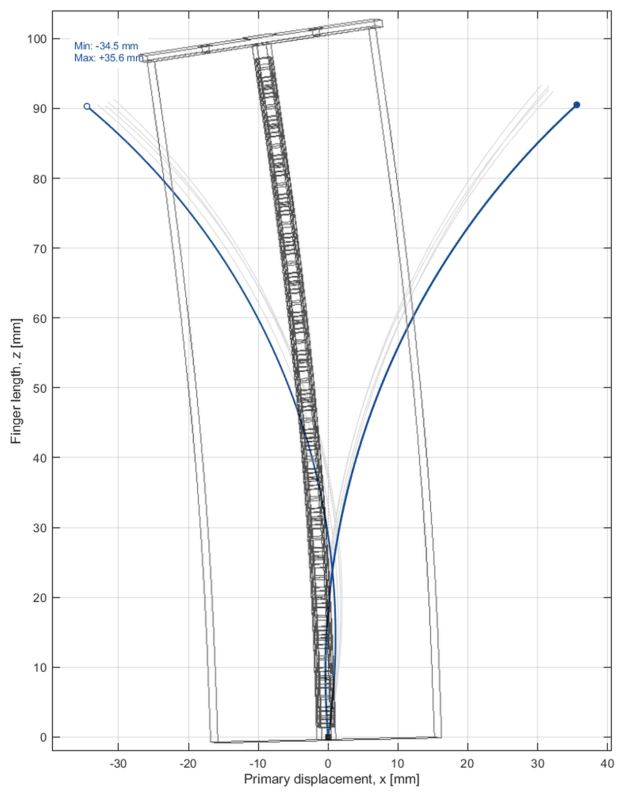
The experimental deformation was measured using an OptiTrack optical motion-capture system, as shown in Figure 4. Three reflective markers were positioned along the actuator to represent the fixed region, the intermediate region, and the fingertip. Their reconstructed three-dimensional positions were used to determine an equivalent bending angle $\theta$. Because bending was experimentally obtained in both directions, the original dataset was evaluated separately for the left and right branches and subsequently summarized by the mean absolute bending angle. The corresponding quantities were defined as

$${\left|\overline{\theta }\right|}_{\mathrm{EXP}}={\displaystyle \frac{1}{n}}{\displaystyle \sum _{i=1}^n}\left|{\theta }_i\right|.$$

(2)

The zero-added-payload condition was selected as the experimental reference because it introduces no additional external mass load that is absent from the present finite element model. For the $t=2.0$ mm configuration, the mean absolute bending angles of the two experimental branches were 60.15° and 48.22°, while the overall mean absolute bending angle was 54.18°. [43]. The difference between the two bending branches is retained in the present analysis as an experimentally observed indication of the non-ideal symmetry of the fabricated soft structure, rather than being replaced by an artificial symmetric value.

2.3. Nonlinear Finite Element Model and Numerical Procedure

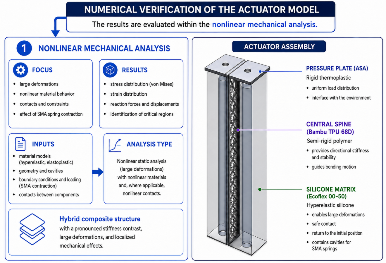
The numerical verification of the design was processed as a set of interconnected FEM analyses. Figure 5 depicts the SOLIDWORKS Simulation 2022 (Dassault Systèmes SolidWorks Corp., Waltham, MA, USA). The aim of this subsection is to create a basis for assessing whether the designed composite composition of the soft effector creates the required deformation and whether unacceptable local stress concentrations arise. The overall goal is to identify morphological computation descriptors. For this reason, the results are divided into four nonlinear studies. The solved assembly is represented by a configuration of three materials: hyperelastic silicone Ecoflex^TM 00-50, semi-rigid polymer Bambu TPU 68D and rigid thermoplastic ASA (acrylonitrile styrene acrylate) FDM thermoplastic (Stratasys, Minnetonka, MN, USA), the parameters of which will be presented in the following sections.

From a mechanical point of view, it is a hybrid composite structure with a significant difference in stiffness, with large deformations, and with local thermo-mechanical effects. This combination determines that the geometric intuitive distribution of the components alone is not enough. This situation indicates that identical external shapes can exhibit significantly different kinematics, stress peaks, and repeatability of shape recovery, depending on how the soft and stiff components are distributed. Therefore, three levels of information were further distinguished when interpreting the results. The first level is the numerical assumptions of the calculation, which include material models, mesh, contacts, boundary conditions, and the choice of solver. The second level is the resulting stresses, displacements, component displacements, and shape deformations. The third level is the interpretation of the design, i.e., the classification of individual studies into the initial, working, developed nonlinear, or diagnostic upper-load mode. In the case of soft structures, one cannot proceed only from the maximum stress value, the shape of the deformation, the direction of movement, the localization of the deformation and the consistency of the reaction forces are equally important.

2.4. Solving a Nonlinear Static Problem

The mechanical part was solved as a nonlinear static problem in incremental form. The equilibrium (3) state at a given step can be written using the residual vector:

$$\mathbf{R}(\mathbf{u},T,\lambda )={\mathbf{f}}_{\mathrm{int}}(\mathbf{u},T)-\lambda {\mathbf{f}}_{\mathrm{ext}}=\mathbf{0},$$

(3)

where $\mathbf{u}$ is the nodal displacement vector, T is the temperature state, $\lambda$ the load ramping parameter, ${\mathbf{f}}_{\mathrm{int}}$ are internal forces arising from the deformation of the material, ${\mathbf{f}}_{\mathrm{ext}}$ are external forces, and $\mathbf{R}$ is a residue, signifying an imbalance between internal and external forces. In mechanical nonlinear studies, the 0 to 30 s interval used can be understood as a pseudo time of load increment and equilibrium branch tracking. A nonlinear static problem seeks the deformation state of a structure in which the internal forces in the material are in equilibrium (4) with the external load. This means that

$${\mathbf{f}}_{\mathrm{int}}(\mathbf{u},T)=\lambda {\mathbf{f}}_{\mathrm{ext}},$$

(4)

In nonlinear statics, the stiffness of a system fluctuates with deformation, contact interactions, material properties, and temperature variations. Consequently, the equilibrium (5) is expressed as a residue:

$$\mathbf{R}(\mathbf{u},T,\lambda )=\mathbf{0},$$

(5)

This means that the solver is looking for a state $\mathbf{u}$ where the residual is zero or sufficiently small according to the set tolerance. The solver does not solve the above Equation (6) all at once, but gradually by Newton–Raphson iteration, in which the tangent stiffness is updated at each step:

$${\mathbf{K}}_{\mathrm{T}}^{\left(i\right)}\Delta {\mathbf{u}}^{\left(i\right)}=-{\mathbf{R}}^{\left(i\right)},$$

(6)

$${\mathbf{u}}^{(i+1)}={\mathbf{u}}^{\left(i\right)}+\Delta {\mathbf{u}}^{\left(i\right)}.$$

(7)

This formulation is suitable mainly because large internal displacements, large deformations and hyperelastic materials change the local directional sensitivity of the model during the loading process. The calculation does not work with a single fixed stiffness matrix, but with its continuously updated tangent representation. For the additively manufactured Bambu TPU 68D reinforcement and ASA pressure pad, a linear-elastic orthotropic material description was used. The numerical properties were assigned directly from the corresponding SOLIDWORKS material definitions used in the present finite element model shown in Table 1. Separate local coordinate systems were assigned to both printed components (Coordinate System1 for the TPU reinforcement and Coordinate System2 for the ASA pressure pad), so that the direction-dependent elastic constants were evaluated in the prescribed local material axes. The constitutive relation can therefore be written as

$${\sigma }^m={\mathbf{C}}^m\left({\epsilon }^m-{\epsilon }_{\mathrm{th}}^m\right),$$

(8)

where ${\mathbf{C}}^m$ is the orthotropic stiffness matrix expressed in the local material coordinate system and ${\epsilon }_{\mathrm{th}}^m$ is the corresponding thermal strain. For a temperature change $\Delta T$,

$${\epsilon }_{\mathrm{th}}^m={\alpha }^m\Delta T.$$

(9)

In the case of Ecoflex^TM 00-50, the hyperelastic Ogden formulation was used. The strain-energy density can be written as

$$W={\displaystyle \sum _{p=1}^N}{\displaystyle \frac{{\mu }_p}{{\alpha }_p}}\left({\overline{\lambda }}_1^{{\alpha }_p}+{\overline{\lambda }}_2^{{\alpha }_p}+{\overline{\lambda }}_3^{{\alpha }_p}-3\right)+W_{\mathrm{vol}}\left(J\right),$$

(10)

where ${\overline{\lambda }}_i$ are the modified principal stretches and $J=\det \mathbf{F}$ describes the volumetric change.

The three-term Ogden coefficient set implemented in the SOLIDWORKS material card was used without numerical modification in all nonlinear studies. In the SOLIDWORKS material definition, the quantities labeled as “Power Coefficients” correspond to the Ogden exponents ${\alpha }_i$, whereas the quantities labeled as “Constants” correspond to ${\mu }_i$. Accordingly, the notation adopted in Equation (10) follows the SOLIDWORKS convention, while the numerical coefficient set originates from the experimental Ecoflex^TM 00-50 fit reported in [43,44]. The complete coefficient set used in the analyses is reported in Table 1.

Table 1. Important material parameters relevant for mechanical analysis.

Material	Model	Key Parameters
EcoflexTM 00-50 1	Hyperelastic–Ogden	$\rho =1070$ kg/m3, $\nu =0.4995$, ${\alpha }_{\mathrm{th}}=2756\times {10}^{-4}$ K−1, Power coefficients $(P_i^{\mathrm{SW}}\equiv {\alpha }_i)$: $\{3.105;3.943;-1.219\}$, Ogden constants ${\mu }_i$: $\{0.0234;0.001;-0.013\}$ MPa
ASA 2	Linear elastic orthotropic	$E_x=E_y=2.1478$ GPa, $E_z=1.945$ GPa, $G_{xy}=0.7565$ GPa, $G_{yz}=0.791$ GPa, $G_{xz}=0.7565$ GPa, $\rho =1016$ kg/m3, ${\nu }_{xy}=0.3854$, ${\nu }_{yz}={\nu }_{xz}=0.3995$, ${\alpha }_x={\alpha }_y=6.938\times {10}^{-5}$ K−1, ${\alpha }_z=6.355\times {10}^{-5}$ K−1
Bambu TPU 68D 3	Linear elastic orthotropic	$E_x=E_y=1.19$ GPa, $E_z=0.60$ GPa, $G_{xy}=0.402$ GPa, $G_{yz}=G_{xz}=0.203$ GPa, $\rho =1260$ kg/m3, ${\nu }_{xy}={\nu }_{yz}={\nu }_{xz}=0.48$, ${\alpha }_x={\alpha }_y={\alpha }_z=1.50\times {10}^{-4}$ K−1

¹ Ecoflex^TM 00-50: The density $\rho =1070$ kg/m³ is consistent with the manufacturer-reported density of $1.07$ g/cm³ for Ecoflex^TM 00-50 [45]. The thermal-expansion input ${\alpha }_{\mathrm{th}}=2.756\times {10}^{-4}$ K⁻¹ was adopted from published thermal characterization of Ecoflex^TM 00-50 [46]. The three-term Ogden coefficient set ${\alpha }_i=\{3.105,3.943,-1.219\}$ and ${\mu }_i=\{0.0234,0.001,-0.013\}$ MPa corresponds to the experimentally fitted Ecoflex^TM 00-50 parameters reported by Zhang et al. [44]. These numerical values were entered directly into the SOLIDWORKS material card used in all nonlinear analyses. In SOLIDWORKS terminology, the entries labelled “Power Coefficients” correspond to the Ogden exponents ${\alpha }_i$, whereas the associated “Constants” correspond to ${\mu }_i$ [47]. The value $\nu =0.4995$ was used as the near-incompressibility parameter in the SOLIDWORKS material definition; SOLIDWORKS recommends Poisson ratios close to 0.5 for nearly incompressible hyperelastic materials [47]. The material card was defined with three active constants ($N=3$); therefore, only the three active $({\alpha }_i,{\mu }_i)$ pairs are reported. ² ASA: The orthotropic elastic constants $E_i$, $G_{ij}$ and ${\nu }_{ij}$, together with the density $\rho =1016$ kg/m³, were adopted from the experimental characterization of FDM-printed ASA reported by Yap et al. [48]. That study investigated ASA with a +45°/−45° raster configuration, consistent with the 45° raster strategy used for the fabricated ASA pressure pad in the present actuator. The thermal-expansion coefficients were taken from the Stratasys ASA material data sheet, which reports mean CTE values of 69.38 μm/(m K) in the XY orientation and 63.55 μm/(m K) in the build-related orientation [49]. ³ Bambu TPU 68D: The density $\rho =1260$ kg/m³ and the directional Young’s moduli $E_x=E_y=1.19$ GPa and $E_z=0.60$ GPa were taken from the technical data for Bambu TPU for AMS (Shore hardness 68D), where mechanical properties are reported separately for the X–Y printing plane and the Z build direction [50]. The value $\nu =0.48$ was adopted as a representative TPU Poisson ratio supported by experimental DIC measurements of thermoplastic polyurethane reported by Xu and Juang [51]. The shear moduli used in the SOLIDWORKS material card were treated as derived orthotropic constitutive inputs consistent with the adopted directional elastic moduli and Poisson ratio rather than as independently measured Bambu-specific quantities. The thermal-expansion coefficient $\alpha =1.50\times {10}^{-4}$ K⁻¹ was adopted as a representative TPU value reported in the thermal-property literature [52].

Table 1. Important material parameters relevant for mechanical analysis.

Material	Model	Key Parameters
EcoflexTM 00-50 1	Hyperelastic–Ogden	$\rho =1070$ kg/m3, $\nu =0.4995$, ${\alpha }_{\mathrm{th}}=2756\times {10}^{-4}$ K−1, Power coefficients $(P_i^{\mathrm{SW}}\equiv {\alpha }_i)$: $\{3.105;3.943;-1.219\}$, Ogden constants ${\mu }_i$: $\{0.0234;0.001;-0.013\}$ MPa
ASA 2	Linear elastic orthotropic	$E_x=E_y=2.1478$ GPa, $E_z=1.945$ GPa, $G_{xy}=0.7565$ GPa, $G_{yz}=0.791$ GPa, $G_{xz}=0.7565$ GPa, $\rho =1016$ kg/m3, ${\nu }_{xy}=0.3854$, ${\nu }_{yz}={\nu }_{xz}=0.3995$, ${\alpha }_x={\alpha }_y=6.938\times {10}^{-5}$ K−1, ${\alpha }_z=6.355\times {10}^{-5}$ K−1
Bambu TPU 68D 3	Linear elastic orthotropic	$E_x=E_y=1.19$ GPa, $E_z=0.60$ GPa, $G_{xy}=0.402$ GPa, $G_{yz}=G_{xz}=0.203$ GPa, $\rho =1260$ kg/m3, ${\nu }_{xy}={\nu }_{yz}={\nu }_{xz}=0.48$, ${\alpha }_x={\alpha }_y={\alpha }_z=1.50\times {10}^{-4}$ K−1

¹ Ecoflex^TM 00-50: The density $\rho =1070$ kg/m³ is consistent with the manufacturer-reported density of $1.07$ g/cm³ for Ecoflex^TM 00-50 [45]. The thermal-expansion input ${\alpha }_{\mathrm{th}}=2.756\times {10}^{-4}$ K⁻¹ was adopted from published thermal characterization of Ecoflex^TM 00-50 [46]. The three-term Ogden coefficient set ${\alpha }_i=\{3.105,3.943,-1.219\}$ and ${\mu }_i=\{0.0234,0.001,-0.013\}$ MPa corresponds to the experimentally fitted Ecoflex^TM 00-50 parameters reported by Zhang et al. [44]. These numerical values were entered directly into the SOLIDWORKS material card used in all nonlinear analyses. In SOLIDWORKS terminology, the entries labelled “Power Coefficients” correspond to the Ogden exponents ${\alpha }_i$, whereas the associated “Constants” correspond to ${\mu }_i$ [47]. The value $\nu =0.4995$ was used as the near-incompressibility parameter in the SOLIDWORKS material definition; SOLIDWORKS recommends Poisson ratios close to 0.5 for nearly incompressible hyperelastic materials [47]. The material card was defined with three active constants ($N=3$); therefore, only the three active $({\alpha }_i,{\mu }_i)$ pairs are reported. ² ASA: The orthotropic elastic constants $E_i$, $G_{ij}$ and ${\nu }_{ij}$, together with the density $\rho =1016$ kg/m³, were adopted from the experimental characterization of FDM-printed ASA reported by Yap et al. [48]. That study investigated ASA with a +45°/−45° raster configuration, consistent with the 45° raster strategy used for the fabricated ASA pressure pad in the present actuator. The thermal-expansion coefficients were taken from the Stratasys ASA material data sheet, which reports mean CTE values of 69.38 μm/(m K) in the XY orientation and 63.55 μm/(m K) in the build-related orientation [49]. ³ Bambu TPU 68D: The density $\rho =1260$ kg/m³ and the directional Young’s moduli $E_x=E_y=1.19$ GPa and $E_z=0.60$ GPa were taken from the technical data for Bambu TPU for AMS (Shore hardness 68D), where mechanical properties are reported separately for the X–Y printing plane and the Z build direction [50]. The value $\nu =0.48$ was adopted as a representative TPU Poisson ratio supported by experimental DIC measurements of thermoplastic polyurethane reported by Xu and Juang [51]. The shear moduli used in the SOLIDWORKS material card were treated as derived orthotropic constitutive inputs consistent with the adopted directional elastic moduli and Poisson ratio rather than as independently measured Bambu-specific quantities. The thermal-expansion coefficient $\alpha =1.50\times {10}^{-4}$ K⁻¹ was adopted as a representative TPU value reported in the thermal-property literature [52].

The purpose of the adopted Ecoflex material definition is to provide a consistent hyperelastic representation of the compliant matrix throughout the complete parametric sequence NS I–IV. The present study is not intended as an independent constitutive identification of Ecoflex^TM 00-50, and the adopted material law is therefore not treated as a stand-alone experimentally calibrated material model. The literature-reported Ogden coefficient values were transferred directly to the SOLIDWORKS modified Ogden material definition without software-specific refitting of the original tensile-test data. Consequently, the adopted Ecoflex representation should be regarded as a literature-informed numerical parameterization. This assumption limits the quantitative interpretation of absolute response magnitudes, while preserving a common constitutive basis for the comparative evaluation of all investigated nonlinear states.

The nearly incompressible character of Ecoflex^TM 00-50 was represented by $\nu =0.4995$, which also increases the sensitivity of the numerical solution to mesh quality and convergence. With the activated large-strain formulation, the kinematics are described by the deformation gradient

$$\mathbf{F}=\mathbf{I}+\nabla \mathbf{u}.$$

(11)

The volume model utilizes translational degrees of freedom (12). The estimated number of translational degrees of freedom for a mechanical mesh including 226198 nodes, prior to the imposition of constraints, is approximately

$$n_{\mathrm{DOF}}\approx 3·226198=678594.$$

(12)

This size of the algebraic system, together with the nonlinear material and geometric response, justifies the use of a direct solver of the Large Problem Direct Sparse type. All mechanical nonlinear studies labeled Nonlinear study I (NS I) to Nonlinear study IV (NS IV) are based on the same geometry and the same basic numerical setup, as shown in Table 2.

Table 2. A compact summary of common mechanical settings for nonlinear studies.

Parameter Area	Settings
Type of problem being solved	Nonlinear–Static; 0–30 s; step 1 s
Geometry nonlinearity options	Large displacement formulation; Large strain option
Thermal effect	Temperature loads included; Zero strain at 298 K
Solver	Large Problem Direct Sparse; Force control; Newton–Raphson
Material model	EcoflexTM 00-50 as a hyperelastic Ogden model; TPU and ASA as orthotropic polymer materials
Boundary conditions	2 fixed surfaces; 1 surface with actuation force and time curve 1
Bonds and contacts of materials	Bonded interactions; the model assumes continuous strain transfer between materials without interface separation
Mesh	Blended curvature-based solid mesh; 226,198 nodes and 142,836 elements, no distorted elements

¹ The action force values depend on the calculation using Equation (13) for each of the nonlinear simulations and their respective control force actions within the defined pseudo-time, Figure 6.

Table 2. A compact summary of common mechanical settings for nonlinear studies.

Parameter Area	Settings
Type of problem being solved	Nonlinear–Static; 0–30 s; step 1 s
Geometry nonlinearity options	Large displacement formulation; Large strain option
Thermal effect	Temperature loads included; Zero strain at 298 K
Solver	Large Problem Direct Sparse; Force control; Newton–Raphson
Material model	EcoflexTM 00-50 as a hyperelastic Ogden model; TPU and ASA as orthotropic polymer materials
Boundary conditions	2 fixed surfaces; 1 surface with actuation force and time curve 1
Bonds and contacts of materials	Bonded interactions; the model assumes continuous strain transfer between materials without interface separation
Mesh	Blended curvature-based solid mesh; 226,198 nodes and 142,836 elements, no distorted elements

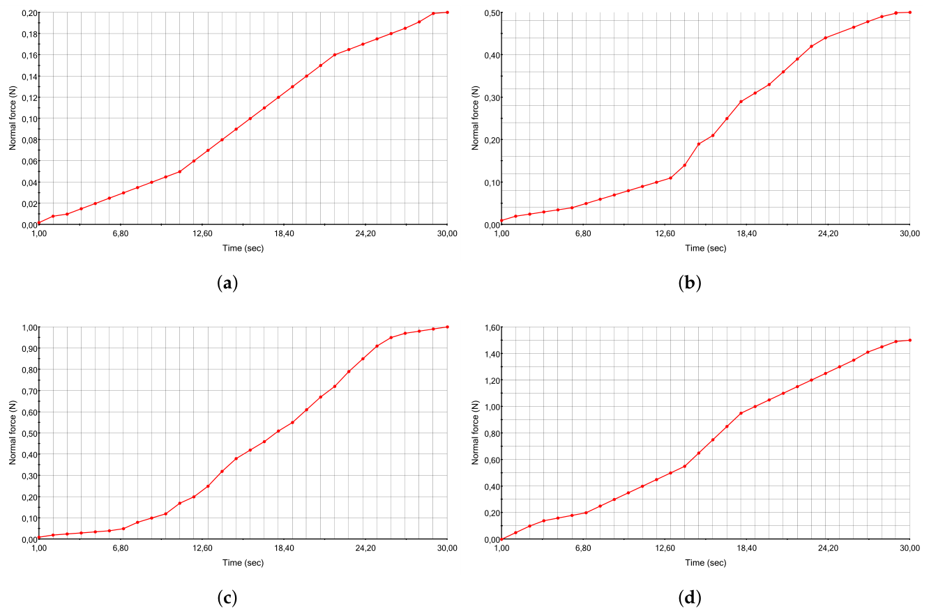
¹ The action force values depend on the calculation using Equation (13) for each of the nonlinear simulations and their respective control force actions within the defined pseudo-time, Figure 6.

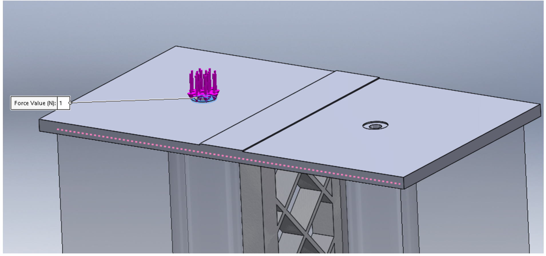
The model is created as a volume mesh with refinement in the areas of geometric transitions, contacts, and assumed local gradients. A rigid clamping is applied to two surfaces, while the actuation load is prescribed on the surface shown in Figure 7. For each nonlinear study, the corresponding final tensile-force level $F_i$ is applied progressively through a dimensionless load-ramping function ${\gamma }_i\left(\tau \right)$ defined over the pseudo-time interval, Figure 6. The instantaneous prescribed actuation force is therefore determined by both the selected force level $F_i$ and its pseudo-time-dependent scaling factor ${\gamma }_i\left(\tau \right)$:

$$F_{\mathrm{ACT},i}\left(\tau \right)=F_i{\gamma }_i\left(\tau \right),$$

(13)

where $F_i$ is the prescribed physical tensile-force level [N] for the corresponding nonlinear study and ${\gamma }_i\left(\tau \right)$ is a dimensionless load factor, with ${\gamma }_i=0$ representing the unloaded state and ${\gamma }_i=1$ the full prescribed load. The corresponding final prescribed force levels for NS I–IV were 0.2, 0.5, 1.0, and 1.5 N, respectively the rationale for their election and their relation to the previous experimental NiTi characterization are specified in Section 2.5.

Figure 6. The calculation of the force that will be applied within the framework of nonlinear static analysis depends on calculation with Equation (13). (a) Normal force values for Nonlinear study I simulation. (b) Normal force values for Nonlinear study II simulation. (c) Normal force values for Nonlinear study III simulation. (d) Normal force values for Nonlinear study IV simulation. (Note: In the graphical representations, decimal commas are used instead of decimal points, e.g., “0,1” stands for “0.1”).

Figure 6. The calculation of the force that will be applied within the framework of nonlinear static analysis depends on calculation with Equation (13). (a) Normal force values for Nonlinear study I simulation. (b) Normal force values for Nonlinear study II simulation. (c) Normal force values for Nonlinear study III simulation. (d) Normal force values for Nonlinear study IV simulation. (Note: In the graphical representations, decimal commas are used instead of decimal points, e.g., “0,1” stands for “0.1”).

Figure 7. The surface on which the action force is defined represents the action effect of the SMA actuator as an NiTi spring in the withdrawal phase.

Figure 7. The surface on which the action force is defined represents the action effect of the SMA actuator as an NiTi spring in the withdrawal phase.

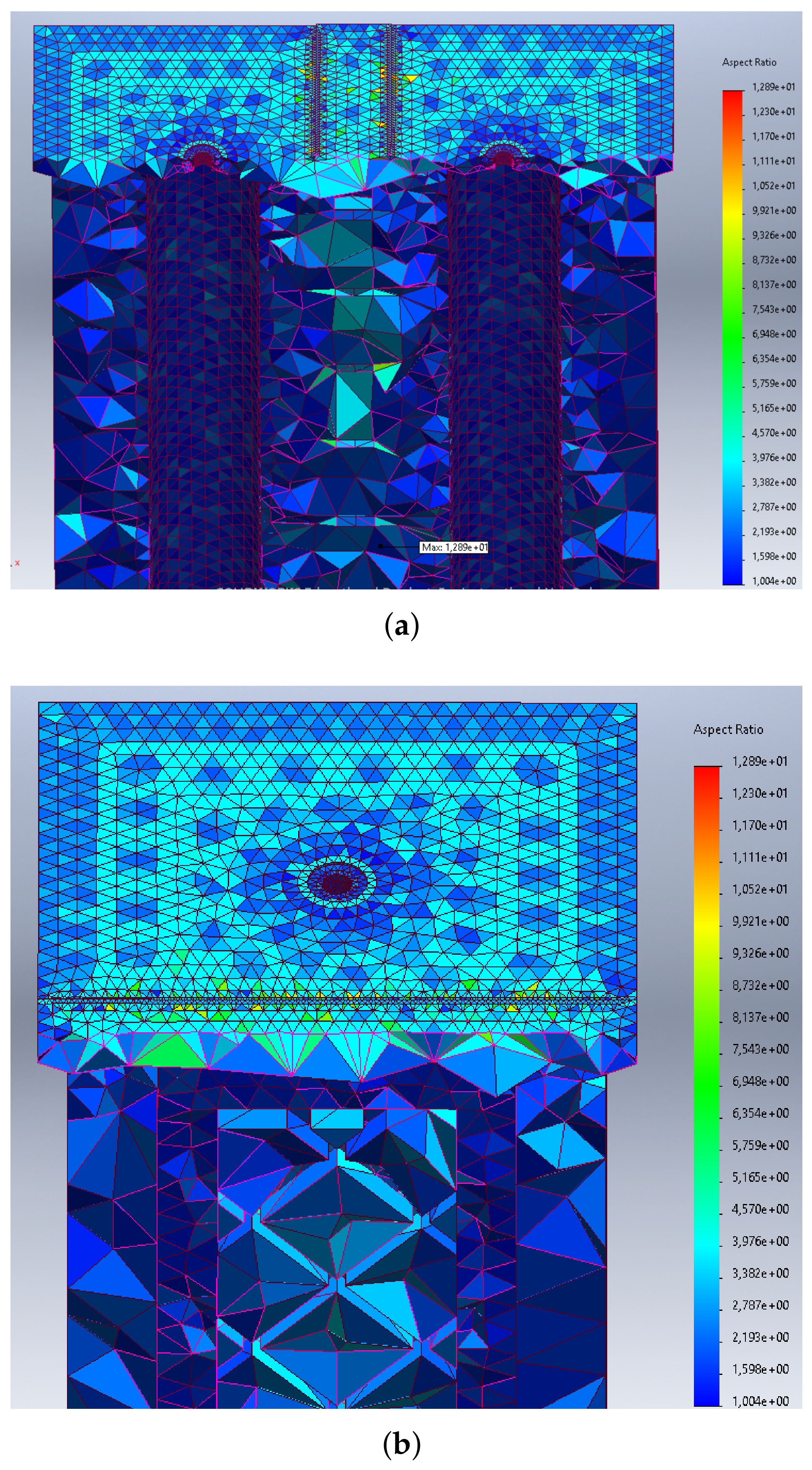
The blended curvature-based mesh used is suitable for curved elastomer bodies and for a combination of stiffer and softer parts. The maximum element size was set at 2.65571 mm, and the minimum size was 0.177046 mm. The proportion of elements with an aspect ratio less than 3 was approximately 95 %, while the proportion of elements with an aspect ratio greater than 10 was only 0.0091 %, which almost minimizes elements with geometric heterogeneity, as shown in Figure 8.

In the displayed meshes, most of the elements are colored in the blue-turquoise range, which means that the aspect ratio is mostly low to medium and the mesh is generally usable for nonlinear mechanical analysis in terms of the shape quality of the elements. Locally increased aspect ratio values appear mainly around thickness transitions, holes, cavities, and the contact area at the upper pad, with the maximum according to the legend reaching approximately 12.893. The reported aspect-ratio statistics constitute a mesh-quality assessment rather than a formal mesh-convergence study. A dedicated mesh-sensitivity analysis is therefore identified as a limitation of the present model. Local mesh controls were used in critical areas, such as points of contact between materials and points where the action force acts, refining the mesh precisely where higher stress or deformation gradients are expected. Also, for the needs of correct numerical processing of the nonlinear problem, more specific parameters of individual materials, Ecoflex^TM 00-50, Bambu TPU 68D, and thermoplastic ASA, were defined, as shown in Table 1.

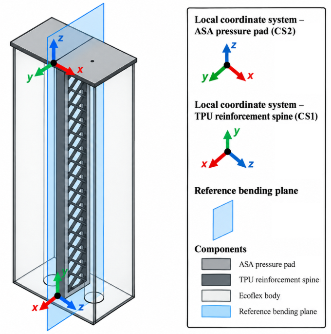
For the additively manufactured Bambu TPU 68D reinforcement and ASA pressure pad, separate local material coordinate systems were defined to correctly assign the direction-dependent properties of the linear-elastic orthotropic models, as in Figure 9. Coordinate System1 was assigned to the TPU reinforcement and Coordinate System2 to the ASA pressure pad. In both cases, the local x–y plane corresponds to the printing-layer plane, whereas the local z axis represents the layer-stacking (build) direction. Because the two components have different manufacturing orientations within the assembly, their local coordinate systems are correspondingly rotated. Consequently, the directional elastic constants listed in Table 1 are applied according to the actual printing orientation of each component. The coordinate-system origins serve only as geometrical reference points, while the orthotropic response is governed by the orientation of the local axes.

The nominal bending plane is defined perpendicular to the symmetric reference bending plane (drawn in blue), Figure 9. In the global coordinate system, this plane corresponds to the X–Y plane and represents the intended dominant deformation path. Displacement within this plane is therefore interpreted as the programmed bending response, whereas the global Z represents the direction with minimum deformation.

Representative Experimental–Numerical Comparison Protocol

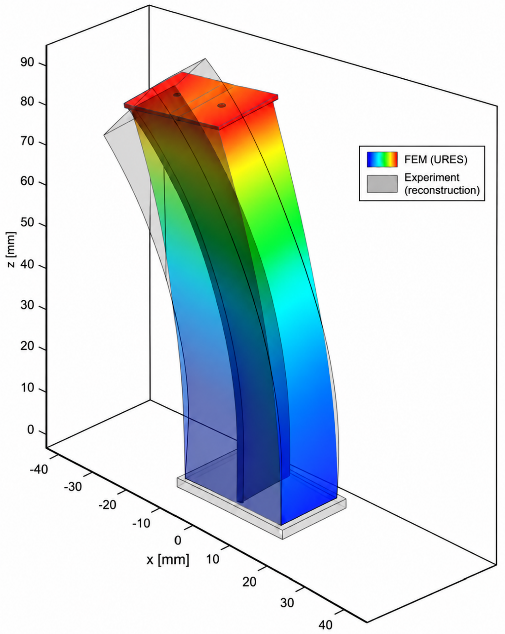
A representative experimental–numerical comparison was performed using Nonlinear Study III. This state was selected a priori, rather than by searching for the numerical result that best matched the experiment. NS III corresponds to a final equivalent mechanical actuation force of 1.0 N and represents a developed nonlinear deformation state while remaining below the highest investigated diagnostic loading condition, NS IV.

NS III was selected as the representative numerical condition because its 1.0 N prescribed actuation level lies within the experimentally investigated mechanical loading scale of the NiTi actuation elements reported in [43]. In the previous characterization, one of the applied mechanical load levels corresponded to approximately 0.981 N. This information is used only to establish a physically informed order of magnitude for the equivalent mechanical input. The comparison is therefore not a force-matched validation, because the instantaneous tensile force generated by the SMA spring was not measured simultaneously during the OptiTrack experiment.

For the numerical comparison, three reference positions corresponding geometrically to the fixed, intermediate, and fingertip marker locations of the OptiTrack measurement were extracted from the deformed NS III configuration. The numerical bending angle ${\theta }_{\mathrm{FEA}}$ was evaluated using the same geometrical processing definition as that used for the experimental marker data. The relative difference in bending angle was then calculated as

$$e_{\theta }={\displaystyle \frac{\left|\left|{\theta }_{\mathrm{FEA}}\right|-{\left|\overline{\theta }\right|}_{\mathrm{EXP}}\right|}{{\left|\overline{\theta }\right|}_{\mathrm{EXP}}}}\times 100\%.$$

(14)

$$\Delta \theta =\left|\left|{\theta }_{\mathrm{FEA}}\right|-{\left|\overline{\theta }\right|}_{\mathrm{EXP}}\right|.$$

(15)

The comparison was therefore not treated as a binary validation criterion based exclusively on agreement in bending-angle magnitude. Instead, two complementary outcomes were evaluated: (i) agreement in the dominant bending direction as an indicator of whether the prescribed morphology establishes the experimentally observed preferred deformation mode, and (ii) agreement in bending magnitude as an indicator of the quantitative predictive capability of the reduced structural model. A disagreement in the second quantity consequently identifies limitations of the adopted model rather than invalidating the assessment of the first quantity.

2.5. Morphological Computational Algorithm Methodology

The morphological calculation of the proposed hybrid soft actuator can be understood as the transformation of the mechanical activation input of one SMA spring into the resulting change in shape, deformation, stress change, and overall stiffness of the actuator. The response of the entire actuator is thus controlled not only by the magnitude of the tensile force but also by the mutual influence of the actuator geometry together with the material distribution and mechanical boundary conditions. The computational morphology is based on a fully symmetric actuator geometry, denoted as $G_{\mathrm{sym}}^{\mathrm{full}}$. This designation expresses that the actuator has a symmetric structural architecture from a geometric point of view. However, physically, the symmetric actuation can be partially disrupted, which can also be a consequence of not completely homogeneous material distribution or direct deformation effects. The structural material set is defined as (16)

$$M_s=\left\{\mathrm{Ecoflex},\mathrm{TPU},\mathrm{ASA}\right\},$$

(16)

where Ecoflex represents a soft silicone-based material for the overall deformable body, TPU represents a locally stiffer material for increased stiffness in the plane of symmetry, and ASA represents a stiffer support or pressure area. The difference in stiffness between these materials forms the basis of the mechanical morphological calculation, as the actuation force is not transmitted uniformly through the structure but is redistributed by the geometry and arrangement of the materials into a specific deformation pattern. The mechanical morphology of the actuator is defined as follows in Equation (17):

$${\mathcal{M}}_{\mathrm{m}}=\left\{G_{\mathrm{sym}}^{\mathrm{full}},M_s,B_{\mathrm{m}},C,A_{\mathrm{SMA}}^{\mathrm{m}}\right\},$$

(17)

where $B_{\mathrm{m}}$ denotes the mechanical boundary conditions, C denotes bonded interfaces between material regions and $A_{\mathrm{SMA}}^{\mathrm{m}}$ denotes the mechanical actuation model of the SMA spring. In the present formulation, ${\mathcal{M}}_{\mathrm{m}}$ denotes the complete mechanical configuration used for response mapping rather than geometry alone. It therefore contains the prescribed geometry and material distribution together with the boundary, interface, and equivalent actuation definitions required to uniquely specify the nonlinear structural problem. These quantities remain fixed throughout NS I–IV; only the final prescribed force level $F_i$ is varied. The equivalent mechanical SMA actuation model is written as Equation (18):

$$A_{\mathrm{SMA}}^{\mathrm{m}}=\left\{{\mathbf{f}}_{\mathrm{ACT}}\left(\tau \right)\right\},\tau \in [0,30\mathrm{s}].$$

(18)

The vector ${\mathbf{f}}_{\mathrm{ACT}}\left(\tau \right)$ represents the mechanical action of the SMA spring in the analyzed pseudo-time $\tau$. In our investigated case, the SMA actuator is represented only by its equivalent mechanical effect, while the thermal effect of the SMA actuator is neglected.

The pseudo-time interval used for the gradual force-control loading process is defined by Equation (19):

$${\mathcal{T}}_{\tau }=\left\{{\tau }_0,{\tau }_1,\dots ,{\tau }_m\right\},0={\tau }_0<{\tau }_1<\dots <{\tau }_m=30\mathrm{s}.$$

(19)

The pseudo-time $\tau$ does not represent a dynamic time response of the actuator. It is used as a continuation parameter describing the gradual increase in the mechanical actuation input in the nonlinear static analysis.

The set of investigated mechanical activation states is expressed by Equation (20):

$$F=\left\{F_1,F_2,\dots ,F_n\right\}.$$

(20)

For the present study, the final prescribed force levels were $F_i=\{0.2,0.5,1.0,1.5\}$ N. These values were defined as experimentally informed parametric inputs for the equivalent mechanical SMA actuation model. They were not obtained from a coupled thermo-mechanical SMA constitutive model and should not be interpreted as instantaneous forces generated by the SMA spring at a prescribed temperature or electrical current. The loading scale was informed by the previous experimental characterization of NiTi actuation elements reported in [43], in which defined mechanical loads were applied and related to force according to $F=mg$. For example, loads of 0.02, 0.05, and 0.10 kg correspond to approximately 0.196, 0.491, and 0.981 N, respectively, providing the experimental basis for the rounded 0.2, 0.5, and 1.0 N levels used in NS I–III. The 1.5 N level in NS IV was introduced as an additional parametric load above the 1.0 N reference level while remaining within the mechanical loading range investigated in the previous experiments. These earlier measurements are used only to establish a physically representative loading scale and do not imply a one-to-one equivalence between the experimentally tested NiTi configuration and the SMA spring represented in the present finite element model. Each force level $F_i$ represents one mechanical activation input and, at the same time, one family of states in the mechanical morphological map.

For each force level $F_i$, the load-ramping function is defined by Equation (21):

$${\gamma }_i:[0,30\mathrm{s}]\to [0,1],{\gamma }_i\left(0\right)=0,{\gamma }_i\left(30\mathrm{s}\right)=1.$$

(21)

The external mechanical force-control input is then written as Equation (22):

$${\mathbf{f}}_{\mathrm{ext},i}\left({\tau }_k\right)=F_i{\gamma }_i\left({\tau }_k\right){\mathbf{b}}_F,{\tau }_k\in {\mathcal{T}}_{\tau },$$

(22)

where vector ${\mathbf{b}}_F$ defines the direction and spatial distribution of the applied force. From the viewpoint of morphological computation, ${\mathbf{f}}_{\mathrm{ext},i}\left({\tau }_k\right)$ is the mechanical input that is transformed by the actuator morphology into the resulting shape state.

The nonlinear mechanical response is represented by the operator in Equation (23):

$$({\mathbf{u}}_{i,k},{\epsilon }_{i,k},{\sigma }_{i,k})={\mathcal{F}}_{nl}\left({\mathcal{M}}_m,{\mathbf{f}}_{ext,i}\left({\tau }_k\right),T_{\mathrm{ref}}\right).$$

(23)

The operator ${\mathcal{F}}_{nl}$ returns the displacement, strain, and stress fields corresponding to the prescribed mechanical input. It returns the displacement field ${\mathbf{u}}_{i,k}$, strain field ${\epsilon }_{i,k}$, stress field ${\sigma }_{i,k}$ and for the force level $F_i$ and pseudo-time step ${\tau }_k$.

For each pair $(F_i,{\tau }_k)$, the displacement response is written as a vector, as in Equation (24):

$${\mathbf{u}}_{i,k}={\left[U_{\mathrm{RES},i,k},U_{X,i,k},U_{Y,i,k},U_{Z,i,k}\right]}^T.$$

(24)

Here, $U_{\mathrm{RES},i,k}$ represents the resulting summary displacement, while $U_{X,i,k}$, $U_{Y,i,k}$ and $U_{Z,i,k}$ describe the directional displacement components of the actuator response.

The scalar equivalent strain descriptor is extracted as Equation (25):

$${\epsilon }_{\mathrm{eq},i,k}=\underset{\mathbf{x}\in \mathsf{\Omega }}{\max }{\epsilon }_{\mathrm{eq},i,k}\left(\mathbf{x}\right),$$

(25)

and the scalar von Mises stress descriptor is extracted as follows in Equation (26):

$${\sigma }_{\mathrm{vM},i,k}=\underset{\mathbf{x}\in \mathsf{\Omega }}{\max }{\sigma }_{\mathrm{vM},i,k}\left(\mathbf{x}\right).$$

(26)

These quantities provide compact scalar measures of the deformation and stress intensity associated with the corresponding morphological state.

The reduced mechanical response descriptor is defined as follows in Equation (27):

$${\mathbf{d}}_{m,i,k}={\left[U_{\mathrm{RES},i,k},\left|U_{X,\min ,i,k}\right|,{\epsilon }_{\mathrm{eq},i,k},{\sigma }_{\mathrm{vM},i,k}\right]}^T.$$

(27)

The resultant support reaction is not used as an independent morphological descriptor. In a force-controlled static solution, the vector sum of the support reactions is an equilibrium quantity that must balance the resultant externally applied load. It is therefore treated only as an equilibrium verification quantity and not as an indicator of morphological intensity, softening, or stability, as in Equation (28). This descriptor selects the main quantities used for constructing and interpreting the mechanical morphological map which consist of resultant displacement, dominant directional displacement, equivalent strain, equivalent stress and reaction force.

$$\sum _{{\Gamma }_c}{\mathbf{R}}_i+{\mathbf{F}}_{\mathrm{ACT},i}\approx \mathbf{0},$$

(28)

where ${\Gamma }_c$ denotes all constrained surfaces. The pseudo-time-dependent effective stiffness is estimated as in Equation (29):

$$k_{\mathrm{eff},i,k}\approx {\displaystyle \frac{\Delta F_i\left({\tau }_k\right)}{\Delta u_{\mathrm{out},i,k}}},$$

(29)

where $u_{\mathrm{out},i,k}$ is a selected output displacement of the actuator. This parameter describes how sensitively the actuator changes its shape when the actuation force changes. A decrease in $k_{\mathrm{eff},i,k}$ indicates progressive softening of the structural response; it is not used as a stability criterion in the present study. The quantity $k_{\mathrm{eff},i}$ is a finite-difference incremental stiffness evaluated between adjacent final force–displacement states. It represents the sampled slope of the global force–displacement response and is distinct from the tangent stiffness matrix used internally by the Newton–Raphson nonlinear solver.

The mechanical morphological state is obtained by the extraction operator in Equation (30):

$${\mathbf{q}}_{i,k}={\mathcal{H}}_{\mathrm{m}}\left({\mathbf{d}}_{\mathrm{m},i,k},k_{\mathrm{eff},i,k}\right).$$

(30)

The operator ${\mathcal{H}}_{\mathrm{m}}$ transforms the selected displacement, strain, stress, reaction force and stiffness descriptors into a compact mechanical morphological state. The quantity ${\mathbf{q}}_{i,k}$ denotes the unclassified mechanical response state extracted from the finite element descriptors. The symbols ${\mathbf{q}}_{\mathrm{init}}$, ${\mathbf{q}}_{\mathrm{work}}$, ${\mathbf{q}}_{\mathrm{dev}}$, and ${\mathbf{q}}_{\mathrm{diag}}$ denote the subsequent ordinal class labels assigned to the final response states and should not be confused with the continuous state vectors ${\mathbf{q}}_{i,k}$. The time-parametrized mechanical morphological map is therefore written as Equation (31):

$${\mathsf{\Phi }}_{\mathcal{M},1}^{\mathrm{m}}:\left(F_i,{\tau }_k,T_{\mathrm{ref}}\right)\mapsto {\mathbf{q}}_{i,k}.$$

(31)

This map describes the transformation of the force-control input into a sequence of shape changes, deformation, stress and stiffness states during the pseudo-time loading process.

For the comparison of the individual nonlinear mechanical studies, the final state at the last pseudo-time step is used, Equation (32):

$${\mathbf{q}}_i={\mathbf{q}}_{i,m}={\mathbf{q}}_i(\tau =30\mathrm{s}),{\mathbf{d}}_{\mathrm{m},i}={\mathbf{d}}_{\mathrm{m},i,m}.$$

(32)

The corresponding final-state morphological map can be written as Equation (33):

$${\mathsf{\Phi }}_{\mathcal{M},1}^{\mathrm{m}}:\left(F_i,30\mathrm{s},T_{\mathrm{ref}}\right)\mapsto {\mathbf{q}}_i.$$

(33)

This final-state map represents the discrete morphological response used for comparing the individual nonlinear mechanical studies.

The set of final morphological states is defined as Equation (34):

$$\mathcal{Q}=\left\{{\mathbf{q}}_1,{\mathbf{q}}_2,\dots ,{\mathbf{q}}_n\right\},$$

(34)

and the corresponding set of final descriptors is as in Equation (35):

$${\mathcal{D}}_{\mathrm{m}}=\left\{{\mathbf{d}}_{\mathrm{m},1}^T,{\mathbf{d}}_{\mathrm{m},2}^T,\dots ,{\mathbf{d}}_{\mathrm{m},n}^T\right\}.$$

(35)

To compare the individual final states, the mechanical response descriptors are arranged into the response matrix (36):

$${\mathbf{D}}_{\mathrm{m}}=\left[\begin{array}{c}{\mathbf{d}}_{\mathrm{m},1,m}^T\\ {\mathbf{d}}_{\mathrm{m},2,m}^T\\ ⋮\\ {\mathbf{d}}_{\mathrm{m},n,m}^T\end{array}\right]=\left[\begin{array}{c}{\mathbf{d}}_{\mathrm{m},1}^T\\ {\mathbf{d}}_{\mathrm{m},2}^T\\ ⋮\\ {\mathbf{d}}_{\mathrm{m},n}^T\end{array}\right].$$

(36)

The columns of this matrix represent the selected mechanical descriptors used to construct and interpret the morphological map.

Because the selected descriptors have different physical units and ranges, column-wise maximum normalization was applied, Equation (37):

$${\widehat{d}}_{i,j}=N_m\left(d_{i,j}\right)={\displaystyle \frac{d_{i,j}}{{\displaystyle \underset{r=1,\dots ,n}{\max }{d}_{r,j}}}},j\in \left\{U_{\mathrm{RES}},\left|U_{X,\min }\right|,{\epsilon }_{\mathrm{eq}},{\sigma }_{\mathrm{vM}}\right\}.$$

(37)

The actuation force was normalized using the same maximum-value principle, as shown in Equation (38):

$${\widehat{F}}_i=N_F\left(F_i\right)={\displaystyle \frac{F_i}{{\displaystyle \underset{r=1,\dots ,n}{\max }{F}_r}}}={\displaystyle \frac{F_i}{1.5\mathrm{N}}}.$$

(38)

This normalized force is used for evaluating the relative deformation response with respect to the mechanical input. No preferential weighting was applied; therefore, $w_U=w_X=w_{\epsilon }=w_{\sigma }=0.25$ and $w_U+w_X+w_{\epsilon }+w_{\sigma }=1$. The intensity of the mechanical morphological response is expressed by the index in Equation (39):

$$I_i^{\mathrm{m}}=w_U{\widehat{U}}_{\mathrm{RES},i}+w_X\left|{\widehat{U}}_{X,\min ,i}\right|+w_{\epsilon }{\widehat{\epsilon }}_{\mathrm{eq},i}+w_{\sigma }{\widehat{\sigma }}_{\mathrm{vM},i}.$$

(39)

The coefficients $w_U$, $w_X$, $w_{\epsilon }$ and $w_{\sigma }$ are weighting factors associated with the normalized displacement, dominant directional displacement, equivalent strain and equivalent stress descriptors. The index $I_i^{\mathrm{m}}$ therefore provides a compact scalar measure of the shape, strain and stress intensity of the corresponding morphological state.

This quantity indicates whether the reaction-force response remains consistent with the increasing deformation state. It is used as a diagnostic parameter and not as the primary measure of morphological intensity.

The degree of nonlinear shape response can be described by Equation (40):

$${\eta }_i^{\mathrm{nl}}={\displaystyle \frac{{\widehat{U}}_{\mathrm{RES},i}}{{\widehat{F}}_i}},$$

(40)

because all evaluated final states satisfy ${\widehat{F}}_i>0$, no numerical regularization term is required in this definition. The indicator ${\eta }_i^{\mathrm{nl}}$ represents normalized deformation response per normalized mechanical input. It is used only as a dimensionless descriptor of the nonlinear force–displacement evolution and should not be interpreted as energetic efficiency, actuator efficiency, or a stability metric.

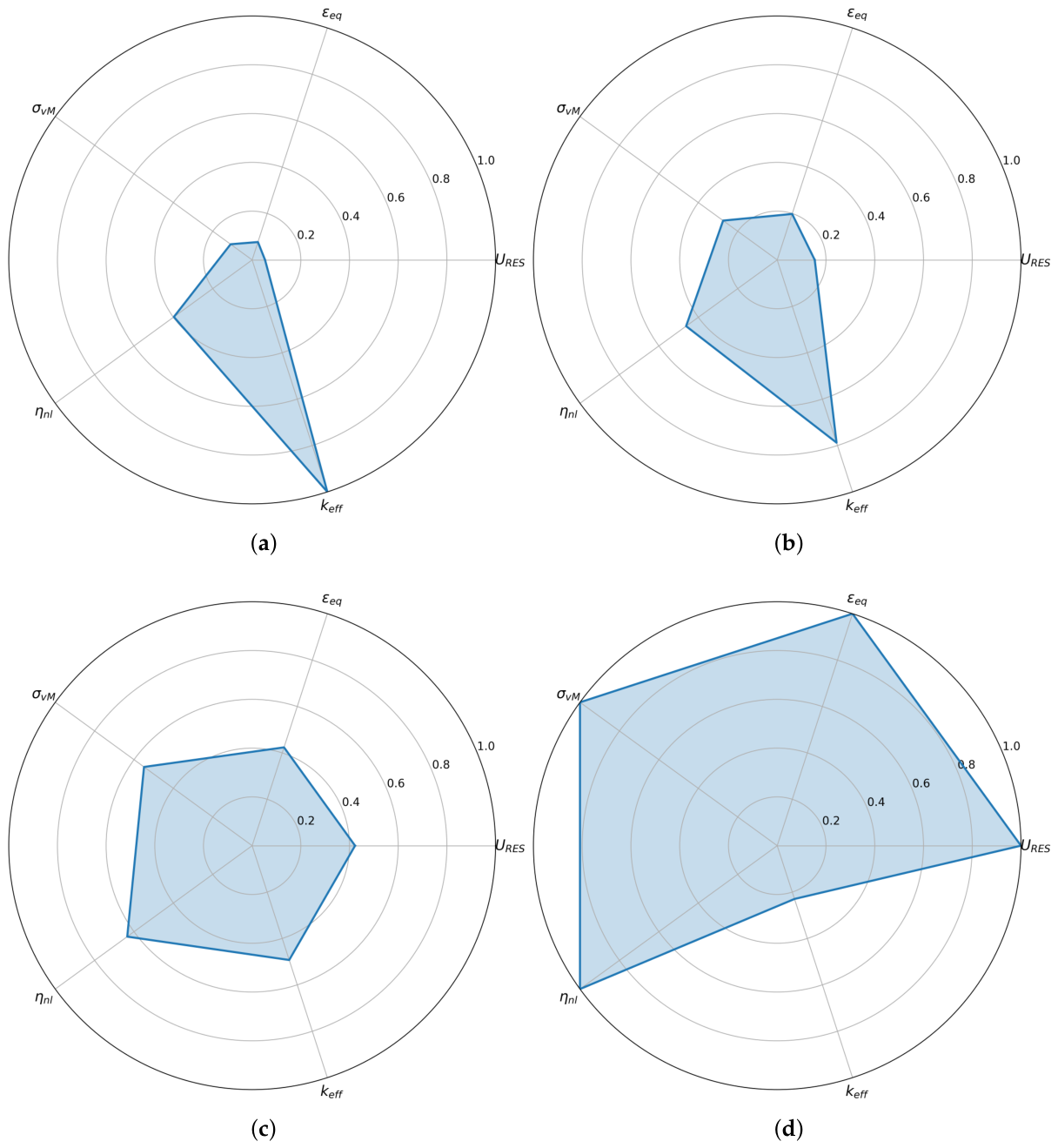
For the present four-state parametric study, the morphological regimes were assigned quantitatively from the mechanical morphological intensity index $I_i^m$. The classification boundaries were defined as the midpoints between the intensity values of adjacent states:

$$b_1=0.1334,b_2=0.3237,b_3=0.7266.$$

(41)

The classification operator is therefore defined as

$$K_m\left(I_i^m\right)=\left\{\begin{array}{cc}{q}_{\mathrm{init}},\hfill & I_i^m\le b_1,\hfill \\ q_{\mathrm{work}},\hfill & b_1<I_i^m\le b_2,\hfill \\ q_{\mathrm{dev}},\hfill & b_2<I_i^m\le b_3,\hfill \\ q_{\mathrm{diag}},\hfill & I_i^m>b_3.\hfill \end{array}\right.$$

(42)

These thresholds provide a reproducible internal classification of the four investigated parametric states and do not represent material-failure, bifurcation, or structural-stability limits. The boundaries $b_1$, $b_2$, and $b_3$ are dataset-internal ordinal classification boundaries defined from the four investigated response states of the reference morphology. They are not universal design thresholds and do not represent material failure, structural stability, bifurcation, or experimentally established operating limits. The resulting set of mechanical morphological regimes is expressed as in Equation (43):

$${\mathcal{S}}_{\mathrm{m}}=\left\{{\mathbf{q}}_{\mathrm{init}},{\mathbf{q}}_{\mathrm{work}},{\mathbf{q}}_{\mathrm{dev}},{\mathbf{q}}_{\mathrm{diag}}\right\}.$$

(43)

The state ${\mathbf{q}}_{\mathrm{init}}$ represents the initial response, ${\mathbf{q}}_{\mathrm{work}}$ represents the functional working regime, ${\mathbf{q}}_{\mathrm{dev}}$ represents the developed nonlinear deformation regime and ${\mathbf{q}}_{\mathrm{diag}}$ the highest investigated nonlinear loading state used for diagnostic comparison; no stability or failure criterion is implied.

Thus, the proposed actuator can be interpreted as a mechanically shape-computational system. The mechanical input represented by SMA actuation is not converted into deformation through a single scalar stiffness, but through the complete mechanical structure morphology. This morphology includes the actuator geometry, material distribution, boundary conditions, bonded interfaces and stiffness parameter elements. It should be emphasized that Algorithm A1 is applied to a fixed reference morphology and therefore does not constitute a topology-optimization or morphology-search algorithm. Its purpose is to map the nonlinear structural response of the prescribed $2.0$ mm-reinforcement configuration over the investigated mechanical input levels and to transform the corresponding finite element outputs into normalized response descriptors and ordinal response states. Accordingly, the variation performed within Algorithm A1 is a variation of the equivalent mechanical actuation input, $F_i=\{0.2,0.5,1.0,1.5\}$ N, while the geometry, material distribution, boundary conditions, and interface definitions remain unchanged. The algorithm therefore characterizes the load-dependent evolution of one prescribed morphology rather than searching the morphological design space.

The influence of morphology itself is evaluated separately by a constant-input comparison between the $2.0$ mm and $3.0$ mm TPU reinforcement configurations. The additional $3.0$ mm reinforcement configuration is intentionally not included in Algorithm A1, because it is not part of the four-state load-response sequence used to construct the reference morphological response map. Instead, it is evaluated separately at the common prescribed force of $0.2$ N as a controlled morphology-sensitivity case. This separation avoids mixing force-induced response changes with geometry-induced response changes. In that comparison, the prescribed force is held at $0.2$ N and the reinforcement thickness is varied. The two analyses are complementary: Algorithm A1 characterizes the load sensitivity of the reference morphology, whereas the additional comparison quantifies morphology sensitivity under an unchanged mechanical input. The complete algorithm is summarized in Algorithm A1.

3. Results

The content of this section is the results obtained during the computational phase of the solvers and Algorithm A1. The results are interpreted by post-processing individual computational tasks depending on the problems being solved.

3.1. Results of Nonlinear Static Analysis

Stated nonlinear mechanical studies Nonlinear study I, II, III, and IV form a parametric sequence showing increasing mechanical activation represented by the activation of the SMA actuator at the analyzed multi-material assembly. Their purpose is to capture the gradual development of the actuator response, starting from the initial deformation and progressing to a more pronounced bending state. This is where the interaction between the silicone matrix the central spine and the upper pressing pad becomes evident. From the obtained general results in the post-processing phase it is possible to assess not only the magnitude of the resulting deformation but also the stress distribution, the localization of critical areas and the deformation pattern.

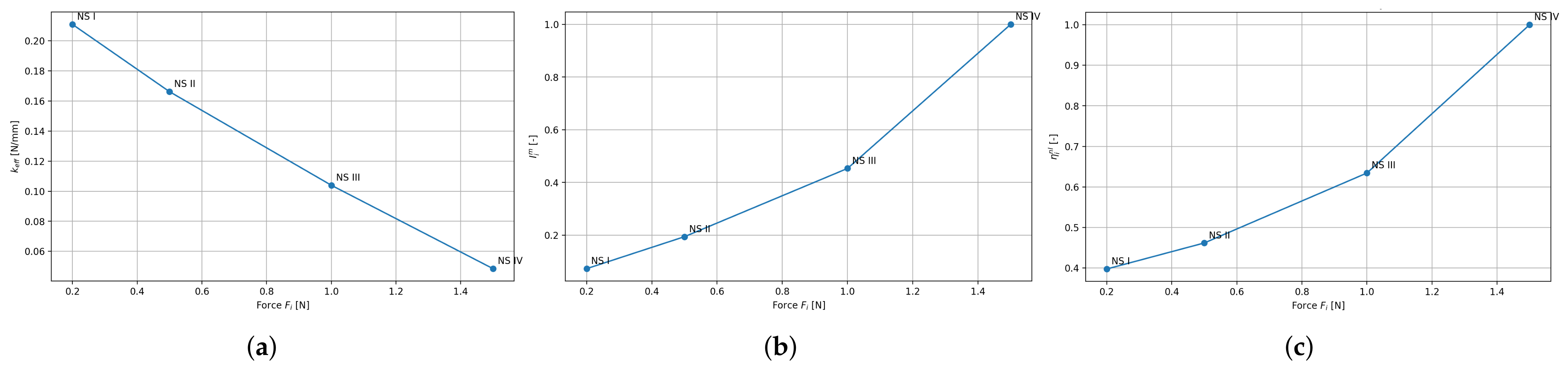
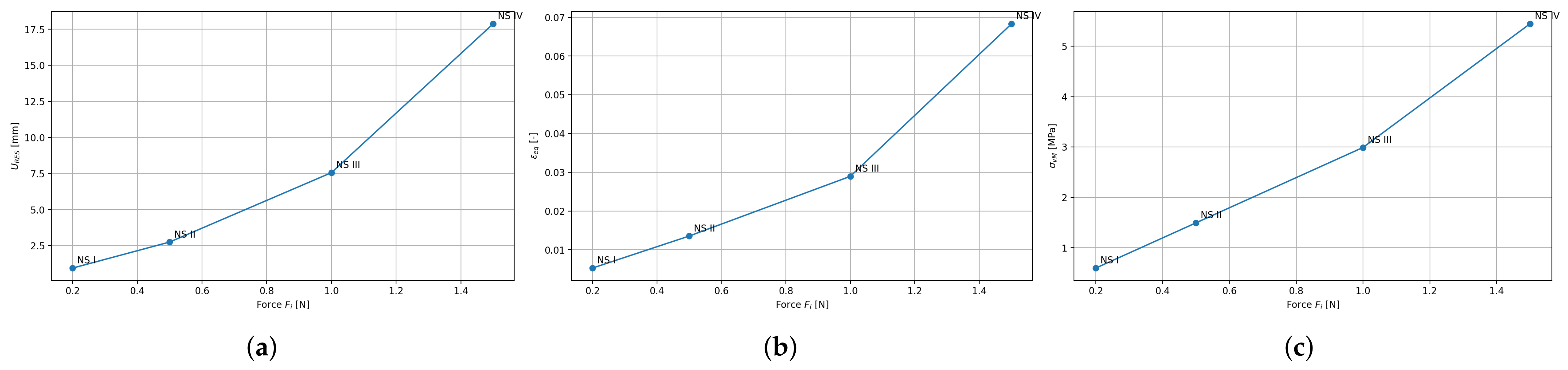
The results of the post-process analysis indicate that the response growth in different cases is significantly nonlinear. An example is the von Mises stress, which increases from approximately 0.596 MPa to 5.447 MPa. The actuator displacements also have nonlinear growth, starting near 0.948 mm and reaching up to 17.88 mm. However, the displacement itself increases from 2.753 mm to 7.562 mm, which indicates nonlinear softening and significant rearrangement of stiffness in the deformed state. The hyperelastic element demonstrates its importance with the results just presented. In general, these results are interesting and therefore we will discuss them in detail below,

Table 3. Summary of key parameters from nonlinear mechanical studies.

Study Type	${\mathit{\sigma }}_{\mathit{vM},\mathit{max}}$ [MPa]	${\mathit{u}}_{\mathit{res},\mathit{max}}$ [mm]	${\mathit{\epsilon }}_{\mathit{eq},\mathit{max}}$ [-]	${\mathit{u}}_{\mathit{x},\mathit{min}}$ [mm]
Nonlinear study I *	0.596	0.948	$5.268\times {10}^{-3}$	−0.905
Nonlinear study II *	1.494	2.753	$1.354\times {10}^{-2}$	−2.651
Nonlinear study III *	2.991	7.562	$2.896\times {10}^{-2}$	−7.373
Nonlinear study IV *	5.447	17.88	$6.833\times {10}^{-2}$	−17.67

* NS I, NS II, NS III, NS IV.

.

3.1.1. Results of Nonlinear Study I

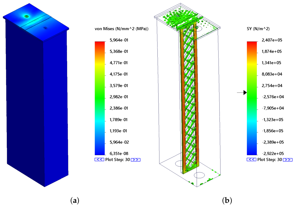
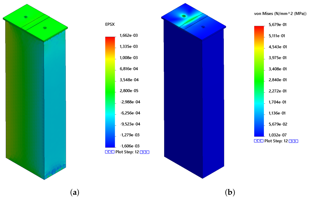
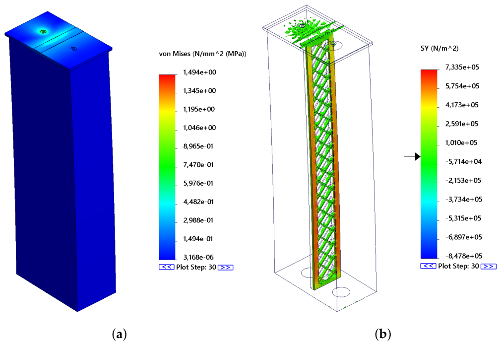
Nonlinear Study I represents the lowest investigated activation level. The maximum von Mises stress of approximately $0.596$ MPa and the maximum resultant displacement of $0.948$ mm show that the response remains substantially below that observed in the higher-load studies. Nevertheless, this calculation is important, as it reflects the basic correctness of the model, such as the orientation of the load, the direction of bending, the functionality of mutual bonds, the behavior of bonded contacts, and also the quality of the mesh. The von Mises stress is localized mainly in the upper pressure plate, at the opening, and in geometric transitions, as shown in Figure 10a. Such a stress distribution was assumed because it is the combination of the opening, changes in material stiffness, and also local force transfer that creates a stress concentrator in the given area. At this lowest investigated activation level, the response remains substantially below that observed in the higher-load studies. On the other hand in Ecoflex, von Mises itself is not a decisive damage criterion because it is a hyperelastic material, and in this case, interpretation via deformations and energy quantities is therefore more important than via the classical linear strength metric. We can therefore conclude that the assembly retains a dominant bending character even with spatial nonlinearity. The normal stress output in the Y-direction shows that, for the analyzed work step, the vertical component of the stress state is mainly concentrated in the circumferential vertical sections of the spine (in red) Figure 10b, while the internal oblique section of the spine mostly displays low SY values. This suggests that the internal spinal system does not primarily transfer load through axial normal stress in the Y-direction, but rather through spatial redistribution of stiffness and shear interaction. The local stress maxima at the superior and inferior ends of the spine are linked to geometric transitions and boundary conditions.

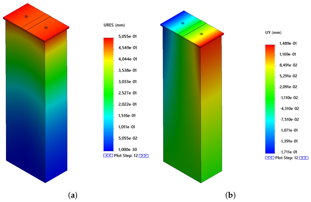
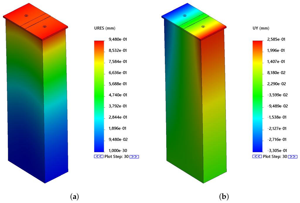
From the analysis results, we can conclude that the graphical field of the resulting global displacement in Figure 11a has a smooth character, and the deformation increases from the lower embedded part towards the upper free area of the effector where the force is considered. Such a distribution is physically expected for the geometry of the bending element. The dominant component of the total motion is the displacement in the X axis. The value $u_{x,min}\approx -0.905$ mm is decisive in terms of functional deflection, while the Y and Z components are of a concomitant nature. The presence of a non-zero displacement in the Y axis indicates a slight transverse asymmetry, which is expected in a multi-material assembly. However, this does not represent a loss of directional control, since the main deformation remains clearly tied to the X axis. The equivalent strain reaches a value of the order of ${10}^{-3}$, which corresponds to a moderate deformation state, as shown in Figure 11b.

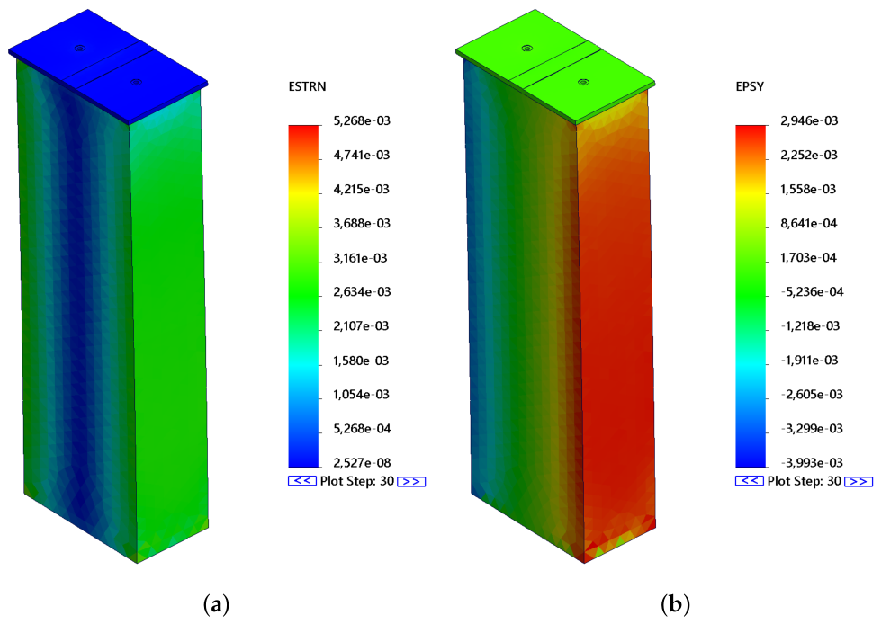
Higher strain values are concentrated in the transition areas between the soft and stiffer parts and in the vicinity of the attachment. The equivalent strain output in Figure 12a showed that the strain intensity stays relatively low in this state and spreads smoothly across the structure’s volume, without notable localization. The highest values appeared around the corners near pad contact. These results thus confirm that Nonlinear study I represents the initial low-load nonlinear response of the actuator. The normal strain output along the Y-axis direction also confirmed that in nonlinear study I, the analyzed element deforms mainly through bending. On one side, positive strain develops, while on the opposite side negative strain forms, which corresponds to the tensile-compressive nature of bending, as shown in Figure 12b.

The study does not reveal any extreme local jumps, possible discontinuities, or unphysical sharp transitions that would indicate an incorrect contact definition or mesh problem. Nonlinear study I can be interpreted as a relevant control within which the displacement and strain fields remain smooth and internally consistent under the adopted numerical assumptions.

3.1.2. Results of Nonlinear Study II

The Nonlinear Study II represents the first mechanically significant operating mode. The maximum resultant displacement of 2.753 mm is already large enough to represent the functional bending of the effector, while the stress of 1.494 MPa and the equivalent strain of $1.354\times {10}^{-2}$ still do not indicate extreme local overloading. Compared to Nonlinear Study I, there is a significant amplification of the response, but without loss of smoothness of the results and while the reported displacement and stress fields remain smooth without abrupt spatial discontinuities. The highest values of von Mises stresses are found mainly in the pressing pad area at the opening and at the geometric transition. The rest of the body remains mostly at low values, which means that the stress concentration is local, not global. This result is critical for the design evaluation. This indicates that, although the actuator exhibits a relatively significant resultant displacement, most of the volume does not experience high equivalent stresses, as shown in Figure 13a. The SY output shows the normal stress in the Y-axis direction, approximately ranging from −0.848 MPa to 0.734 MPa. The stress distribution map shows that the vertical normal stress is more significantly concentrated in the lateral vertical parts of the reinforcement. The internal oblique interconnected structure of the reinforcement remains largely close to the green values, i.e., in the vicinity of the lower or transitional stress state. This means that the internal reinforcement probably does not transmit the load dominantly as pure normal stress in the Y-axis but rather through shear, local stiffness changes, and spatial deformation. From a design perspective, however, it is important that the stress is not evenly distributed throughout the volume but is concentrated in certain load-bearing areas. This confirms the hybrid nature of the actuator, where the soft material allows deformation while the stiffer parts take over the load, as shown in Figure 13b.

The key aspect of this study lies in the ratio between the resulting displacement and the X component. The values $u_{res,max}=2.753$ mm and $u_{x,min}=-2.651$ mm indicate that the dominant portion of the total deformation is carried by the working bend along the X axis. The color field of the X component shows an almost monotonic progression from the clamping area to the free part, typical of a controlled bending effector. The Y and Z components are present, though their role is limited, illustrating the spatial coupling of the deformation rather than a disruption of the main movement direction. The displacement rises steadily from the bottom to the top, with the maximum located in the upper pressing pad area.

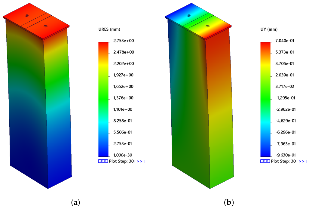
This distribution corresponds to a bent element with one relatively stiffer or less mobile region and another showing the greatest deflection. The resultant displacement increases to 2.753 mm while the spatial field remains continuous under the adopted numerical assumptions. The URES field appears smooth, without abrupt local variations. This suggests that the structure behaves stably and that the deformation spreads through the entire volume rather than concentrating in one critical spot, as shown in Figure 14a. The UY output displays the displacement component along the Y axis ranging from −0.963 mm to 0.704 mm. This finding is significant because it demonstrates that in the Nonlinear Study II, the lateral or transverse displacement part is no longer negligible. The color field exhibits a clear asymmetry, where one part of the upper region reaches positive values and the other negative ones. This indicates that the actuator no longer moves in a single ideal bending direction but begins to exhibit a spatial deformation pattern, as illustrated in Figure 14b. Compared to the Nonlinear Study II, the displacement is significantly higher, indicating that an increased activation produces a larger shape change while preserving a smooth deformation field.

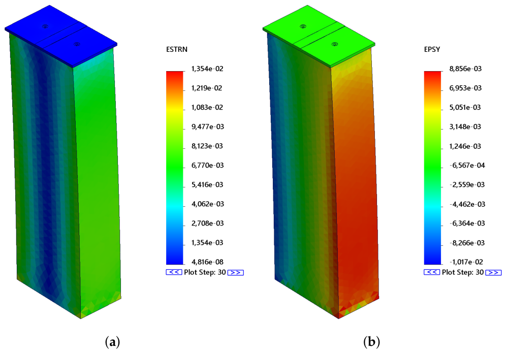
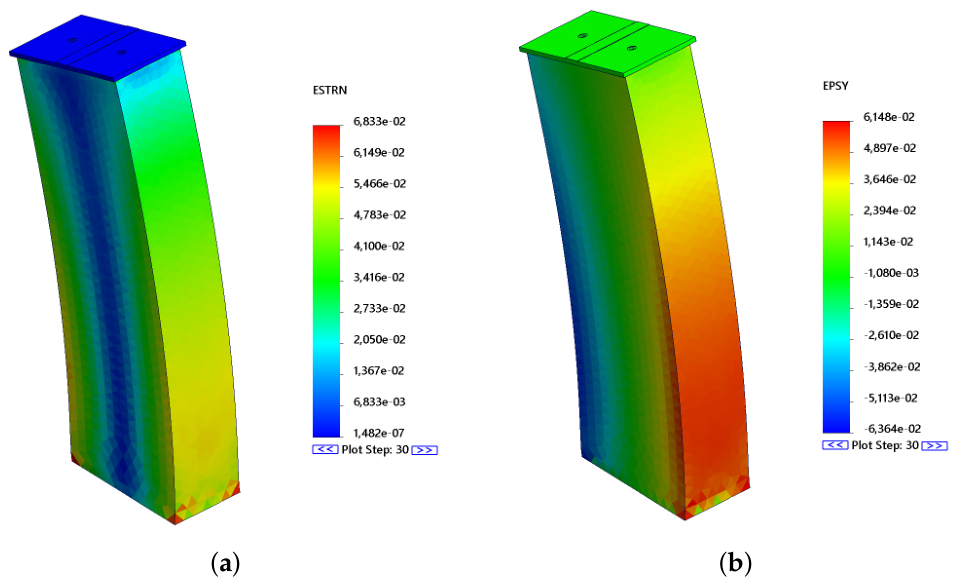
The ESTRN output shows the equivalent, that is, the resulting strain intensity max, $1.354\times {10}^{-2}$. From the strain perspective, Nonlinear Study II is significant because the active deformed zone expands compared with Nonlinear Study II, yet it still remains clearly interpretable. The equivalent strain field appears smooth, and the highest values are located in the transition areas, where the softer volume deforms in interaction with the stiffer embedded parts. The component strains follow the classic bending principle, where one side of the cross-section is in tension while the other is in compression, Figure 15a. The EPSY output displays the normal strain in the Y-axis direction. The range of values is roughly from $-1.017\times {10}^{-2}$ to $8.856\times {10}^{-3}$. On one side of the body, a region of positive strain forms, meaning the tension side, while the opposite side shows negative values, that is, the compression region. This confirms that the actuator continues to deform mainly in a bending manner. The transition between the tensile and compressive sides is smooth, which is a positive indication, as the deformation does not fragment into a local break or sudden singularity. From the actuator’s point of view, this output matters because it demonstrates that at Nonlinear Study II the deformation is no longer only mild but a more distinct tensile-compressive regime begins to develop. In this way, the design efficiently converts the internal or external actuation force into a shape change, as seen in Figure 15b.

3.1.3. Results of Nonlinear Study III

Nonlinear Study III represents a more advanced nonlinear operating state of the actuator. Compared with NS II, all major quantities have risen noticeably. For example, the resulting displacement increased from about 2.753 mm to 7.562 mm, the equivalent strain from roughly $1.354\times {10}^{-2}$ to $2.896\times {10}^{-2}$, and the maximum von Mises stress from around 1.494 MPa to 2.991 MPa. From the actuator’s functional perspective, the key point is that the structure still maintains a recognizable bending mode. Yet, the EPSY and UY outputs indicate that at this load level, a more pronounced spatial deformation already appears. The actuator thus acts as a hybrid, shape-controlled system rather than a simple linear bending beam. From a design viewpoint, Nonlinear Study IV can be described as a state showing a strong functional shape response, though with a growing risk of local concentrations. The critical regions are mainly found at the top pressing plate, near the holes, and near the bottom transitions. These results therefore support interpreting the actuator as a morphologically controlled structure. The larger shape change results from the soft body and hybrid architecture, while the stress peaks remain concentrated in the stiffer and geometrically sensitive zones of the support spine.

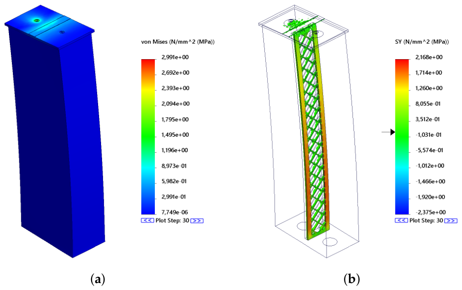
The output of the von Mises analysis indicates an equivalent stress 2.991 MPa, whose value is nearly twice that of Nonlinear Study III. Geometrically, as shown in the Figure 16a, the highest values are concentrated in the region of the upper pressure plate, the support spine, and particularly around the hole. The rest of the body remains mostly at low von Mises stress values. This finding is significant because it again demonstrates that the greatest shape change and the maximum stress do not occur in the same spatial location. The global displacement extends across the entire height of the actuator, while the stress peak is localized and linked to a structural detail. For stiffer materials, especially ASA and TPU, the von Mises stress serves as a reliable indicator of potential risk points. In contrast, for the elastic Ecoflex, this output should be viewed only as supplementary and always considered together with the ESTRN, EPSY, and main strain values. For this reason, ISO clipping is also applied here to identify stress peaks. On Figure 16b, visual SY output shows normal stress in the Y-direction. The range of values goes from −2.375 MPa to 2.168 MPa. This marks a clear increase in the normal stress in the Y-direction compared with the Nonlinear 3 study, where the range was about −0.848 MPa to +0.734 MPa. The visual ISO clipping map indicates that the tensile stress is mainly concentrated in the vertical support strips and in the areas around the internal reinforcement, similar to the earlier cases. The internal oblique reinforcement stays mostly within the green values, meaning it lies near the transition region, but this observation should not be taken as an indication of zero stress. Instead, it suggests that it does not carry the dominant net normal stress in the SY component. Its function is likely tied to shear interaction, stiffness redistribution, and deformation guidance. More distinct local variations appear in the upper part near the plate, the opening, and the transitions between materials. These zones are critical with respect to tensile stress concentration.

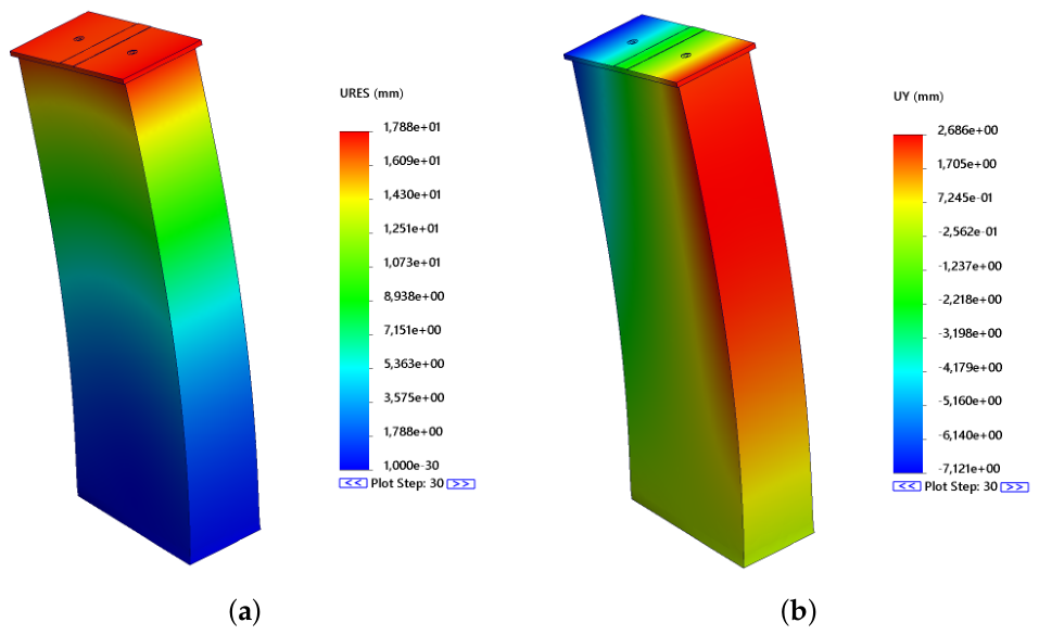
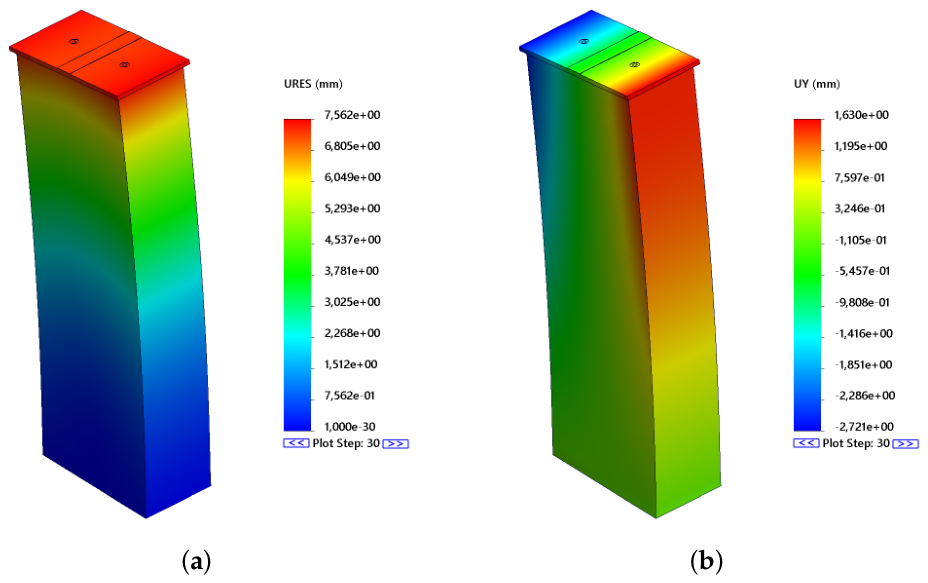
The URES output graph in the Figure 17a shows the total resulting displacement. The maximum value of the total displacement is 7.562 mm. In comparison with the NS II, where the maximum resulting displacement reached about 2.753 mm, this corresponds to roughly a 2.7-fold increase. The actuator therefore demonstrates a notable shape change in this state. The URES map displays a smooth gradient from the bottom to the top, with the maximum located in the region of the upper pressure plate and the upper part of the soft body, which is fully tilted in the respective direction. It is important to note that this large shape change is not accompanied by a chaotic displacement field. The solution remained converged and the displacement field remained spatially continuous throughout the prescribed loading sequence; no structural stability criterion was evaluated. The URES field remains smooth and mechanically interpretable despite the substantially increased global bending. The UY output in the Figure 17b shows the displacement component along the Y axis. The range of values is approximately from −2.721 mm to 1.630 mm. When compared with the Nonlinear 3 study, where the range was about from −0.963 mm to 0.704 mm, this represents a clear increase in the lateral component of motion. The color field indicates that one section of the upper region deflects in the positive Y direction, while the opposite region moves toward negative values. This suggests that the actuator no longer performs a simple planar bending but instead shows a more distinct spatial deformation component. Such behavior can result from asymmetric stiffness distribution, the position of the actuation force, internal reinforcement, and the interaction between the soft and stiff parts of the assembly. From a design standpoint, this outcome is important mainly because if the actuator’s purpose is to achieve a purely planar bend, then the displacement UY highlights the actual lateral deflection, which may require limitation. However, if the aim is a spatial shape response, then UY can be interpreted as a functional expression of the morphological design. In either case, the result is a significant finding, as it demonstrates that at higher levels of actuator activity, the actuator can no longer be regarded as a simple one-dimensional bending element.

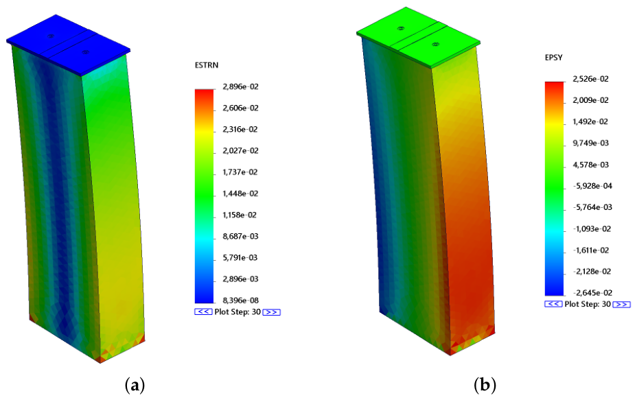
The graphical output of the ESTRN analysis displays the total intensity of the strain in any direction. The peak value is $2.896\times {10}^{-2}$. Interestingly, this is over double the maximum equivalent strain from Nonlinear II, which was about $1.354\times {10}^{-2}$. It seems Nonlinear study III. indicates a more developed nonlinear state. Yet, pinpointing the threshold for this classification is less straightforward than it seems. As shown in Figure 18a, the upper pressure plate mostly exhibits low strain values meanwhile, the majority of the actuator’s soft body displays medium strain values. Increased values, by contrast, seem to appear mainly in the lower areas and at the edge of actuator and the deformation remains distributed across the entire volume. Its clear that the soft material arguably assumes primary responsibility for shape transformation, whereas the stiffer components serve to stabilize and guide that process. Figure 18b presents the EPSY graphic output, depicting normal strain along the Y-axis. Values span roughly from $-2.645\times {10}^{-2}$ to around $2.526\times {10}^{-2}$. The graphic map looks like pronounced bending pattern, with one side of the actuator showing positive strain values and the other side showing compression. Thus, the geometry of the actuator seems to start have set up the asymmetric load distribution that is arguably characteristic of flexural mechanisms. Tension and compression zones are clearly delimited across the cross-section. The EPSY field shows what looks like a coherent structure rather than fragmented isolated areas. Strain varies uniformly across the width of the body.

3.1.4. Results of Nonlinear Study IV

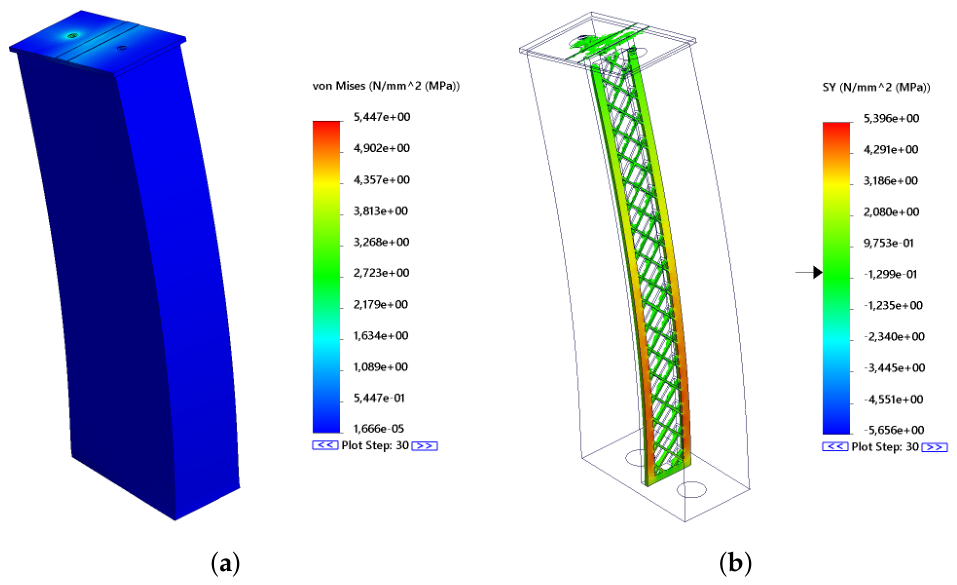
Nonlinear study IV exhibits the most significant deformation when compared to the other studies. Displacement increases from 7.562 mm to 17.88 mm, equivalent strain from 2.896% to 6.833%, and von Mises stress from 2.991 MPa to 5.447 MPa compared to nonlinear study III. Nonlinear study IV represents the strongest nonlinear deformation among the investigated load cases. No formal stability or physical failure criterion was evaluated. Mechanically, the actuator operates in a strongly nonlinear regime. The EPSY, UY, and URES outputs indicate global and smooth deformation, suggesting functional usability. SY and von Mises stress outputs show higher stress concentrations in localized regions, such as the top plate, openings, and longitudinal support strips, similar to earlier cases. The significance of these similarities remains a question.

The output of the von Mises analysis shows a maximum stress value of 5.447 MPa. This represents a notable increase when compared to the Nonlinear Study III, where the maximum was approximately 2.991 MPa. In Figure 19a, it can be seen that most of the actuator volume remains at low von Mises stress values. The highest values appear locally in the area of the upper pressure plate and also in the support spine. This suggests that the stress maximum is mainly tied to local concentration rather than areal overloading of the entire soft body. This is a strong case in favor of the principle of morphological calculation, where the shape response doesn’t arise only because of the high stress state but as a result of appropriately designed geometry, chosen soft material, and reinforcement of the support spine.

The SY output on Figure 19b shows the normal stress on the Y-axis direction. The range of SY values is from −5.656 MPa to 5.396 MPa. This is again a more than twofold increase compared to Nonlinear Study III, where the SY stress was approximately −2.375 MPa to +2.168 MPa. This result indicates that the normal stress in the longitudinal direction is already quite elevated in Nonlinear Study IV. It’s clearly visible in the SY map that the stress is concentrated mainly in the vertical lateral bands in the area of the internal spinal support system. The difference between the SY and URES outputs appears to be important, though not always straightforward. While URES shows a large global shape change, SY shows that the stress loading is spatially selective.

Within the URES output from the nonlinear study, a notable global shape change can be seen in Figure 20a, where the maximum displacement value reaches 17.88 mm. Compared to Nonlinear Study III, where the resulting displacement was about 7.562 mm, the URES output represents more than a two-fold increase. When compared to Nonlinear Study II, where the displacement was around 2.753 mm, the increase is already roughly six-fold. The URES graphic map shows a smooth gradient from the bottom to the top. The maximum appears in the upper part of the actuator, especially around the upper pressure plate. This indicates that the lower area acts as a more constrained region, while the upper part undergoes the largest shape change, showing that the structure can produce a large global deformation. However, it is important that this large resulting displacement is not paired with an equally extensive area of high stresses. This suggests that much of the shape transformation occurs due to the soft morphology of the body, rather than local material overload.

The UY output in Figure 20b presents the displacement component along the Y-axis direction. The range of values extends from −7.121 mm to 2.686 mm. Compared to Nonlinear Study III, where the range was roughly from −2.721 mm to +1.630 mm, the increase in negative displacement is quite significant. This shows that in Nonlinear Study IV, a substantial lateral deflection is already present. The figure reveals that the upper part of the actuator and one side reach high positive values, while the opposite side shifts into strongly negative values. Such a pattern highlights the spatial nature of the deformation. The actuator does not behave merely as a simple beam bent in one plane, but its shape response includes a marked three-dimensional component. From a design perspective, this output can be interpreted in two ways. If the goal was to achieve a pronounced spatial shape response, then UY serves as clear evidence of the morphological design’s functionality. On the other hand, if the goal was to precisely control the actuator’s planar motion, such a large UY value would suggest the need for additional guidance, adjustment of reinforcement stiffness, or geometric symmetrization of the actuator.

The graphical output of the ESTRN analysis shows the total strain intensity in any direction, as shown in Figure 21a. The maximum calculated value of the strain for Nonlinear Study IV is $6.833\times {10}^{-2}$, which corresponds to 6.83%. This represents a notable increase compared to Nonlinear Study III, where the maximum was around 2.896%. This outcome confirms that the Nonlinear Study already captures the advanced working state of the actuator, where the soft material takes over much of the shape change. The ESTRN graphical map indicates that the upper pressure plate remains at low strain values by default, confirming its transmission and stabilization role. In contrast, most of the strain is concentrated in the soft body, mainly in the sides and bottom area. It is important that the deformation is not evenly distributed throughout the volume but follows the bending mechanism and the known material-geometric asymmetry of the structure, caused by imperfections in the manufacturing process.

The EPSY graphic output displays the normal deformation along the Y-axis direction, as shown in Figure 21b. The deformation values in the figure range approximately from $-6.364\times {10}^{-2}$ to $6.148\times {10}^{-2}$. The deformation values cause deformation of the structure from −6.36% to +6.15%. This is a considerable increase in magnitude compared to the Nonlinear III study, where the EPSY deformation was about −2.65% to +2.53%. However, the graphical deformation map still retains a distinctly identifiable bending character. It can also be observed that one side of the actuator works mainly in tension and the other in compression, meaning positive strain values appear on the right side of the body, while negative values occur on the left. We can thus conclude that a tension-compression gradient forms across the actuator’s cross-section. At the same time, it is evident that in the Nonlinear IV study, the deformation is no longer just a slight bending but a marked shape transformation. In the lower region, locally increased values appear, possibly related to placement, boundary conditions, the geometry of the lower part, or local condensation of deformation in areas where movement is structurally limited. This graphic output therefore indicates that the actuator is entering a regime of pronounced nonlinear deformation, yet the strain field retains a spatially coherent bending-related pattern.

3.1.5. Representative Experimental–Numerical Comparison

To provide a quantitative experimental benchmark for the nonlinear structural model, the NS III deformation was compared with the existing OptiTrack measurements of the fabricated P5 actuator with a 2.0 mm TPU reinforcement under zero added external payload. The experimental dataset contained ten recorded states and yielded an overall mean absolute bending angle of ${\left|\overline{\theta }\right|}_{\mathrm{EXP}}=54.18°$. The mean absolute values of the two experimental bending branches were 60.15° and 48.22°.The experimentally reconstructed deformation paths for the two bending directions are shown in Figure 22.

Using the corresponding virtual reference positions in the NS III finite element model, the numerical bending angle was determined as $\left|{\theta }_{\mathrm{FEA}}\right|=9.83°$. The difference in deformation amplitude is also evident from the direct comparison of the numerical and experimentally reconstructed configurations shown in Figure 23. The absolute difference between the experimental mean and the numerical prediction was therefore 44.35°,

Table 4. Representative comparison of the bending response of the fabricated P5 actuator and the NS III finite element model.

Quantity	Experiment	FEA NS III	Difference
Mean absolute bending angle [deg]	54.18	9.83	44.35 (81.86%)

. According to Equation (14), this corresponds to a relative difference of 81.86%. The comparison demonstrates that the finite element model substantially underpredicts the deformation amplitude of the fabricated actuator for the selected representative condition. However, the numerical deformation remains oriented in the same intended dominant bending direction as the experimental response. Consequently, the present comparison supports the qualitative prediction of the preferred bending mode but does not demonstrate quantitative agreement in bending magnitude. The force-controlled finite element representation should therefore not be interpreted as a quantitatively calibrated model of the complete SMA-actuated prototype.

The experimental value represents the mean absolute bending angle from ten OptiTrack records of the $t=2.0$ mm P5 prototype under zero added external payload. The relative difference is calculated with respect to the experimental mean value.

The magnitude of the observed discrepancy is itself an important diagnostic result. The relative difference of 81.86% clearly demonstrates that the present force-controlled finite element model does not quantitatively reproduce the bending amplitude of the fabricated actuator. At the same time, the numerical and experimental configurations exhibit the same intended dominant bending direction. The comparison therefore separates the predictive capability of the model into two levels: the preferred deformation mode is qualitatively reproduced, whereas the deformation magnitude is not.

This distinction is relevant to the morphological interpretation of the actuator. The agreement in dominant bending direction, despite the substantial difference in bending amplitude, supports the interpretation that the prescribed material–geometric architecture biases the structural response toward a preferred deformation path. Conversely, the large amplitude discrepancy shows that the magnitude of this response cannot be attributed to the prescribed morphology alone and remains strongly dependent on material calibration, the actual SMA force–stroke behavior, interface conditions, and manufacturing-related effects that are not fully represented in the present model.

3.2. Morphology-Guided Response and Design-Level Interpretation of the FEA Fields

The quantities introduced in Equations (12)–(38) should not be interpreted as substitutes for the conventional nonlinear finite element solution. Displacement, strain, stress, and reaction force remain direct outputs of the nonlinear FEA model. The purpose of the proposed morphological computation framework is instead to transform these spatially distributed fields into a consistent set of design-level response descriptors that can be related to the geometry, material configuration, and applied mechanical input. Accordingly, the methodological contribution of the framework is not an additional constitutive or equilibrium model, but an interpretation layer that makes it possible to evaluate whether a given structural configuration promotes the intended deformation mode and to compare this response consistently between load states and morphological variants.

To illustrate this distinction quantitatively, a representative response of the actuator with a reinforcement thickness of $t_r=3\mathrm{mm}$ at an applied force of $F=0.2\mathrm{N}$ was examined in detail. The corresponding displacement, directional displacement, normal-strain, and von Mises stress fields are shown in Figure 24 and Figure 25. The deformation scale in all displacement plots is unity.

The maximum resultant displacement obtained for this configuration was

$$U_{\mathrm{RES},\max }=0.5055\mathrm{mm}.$$

(44)

For the applied load, this corresponds to an effective secant compliance

$$C_{\mathrm{eff}}={\displaystyle \frac{U_{\mathrm{RES},\max }}{F}}={\displaystyle \frac{0.5055}{0.2}}=2.5275\mathrm{mm}{\mathrm{N}}^{-1},$$

(45)

and, equivalently, to an effective secant stiffness

$$K_{\mathrm{eff}}={\displaystyle \frac{F}{U_{\mathrm{RES},\max }}}=0.3956\mathrm{N}{\mathrm{mm}}^{-1}.$$

(46)

These quantities reduce the displacement field to a scalar mechanical descriptor that can subsequently be compared between morphological configurations without replacing the underlying nonlinear FEA solution. The Y-direction displacement ranged from $-0.1711\mathrm{mm}$ to $+0.1489\mathrm{mm}$, giving a full-field directional displacement span of

$$\Delta U_Y=U_{Y,\max }-U_{Y,\min }=0.3200\mathrm{mm}.$$

(47)

The maximum absolute Y-component was therefore $0.1711\mathrm{mm}$. Relative to the maximum resultant displacement, the directional displacement ratio becomes

$${\eta }_Y={\displaystyle \frac{\max |U_Y|}{U_{\mathrm{RES},\max }}}={\displaystyle \frac{0.1711}{0.5055}}=0.3385.$$

(48)

Thus, approximately $33.9\%$ of the maximum resultant displacement is represented by the maximum absolute Y-component. In combination with the coordinate-system definition introduced for the actuator model, this descriptor provides a quantitative measure of deformation directionality. If the Y axis is defined normal to the intended bending plane, ${\eta }_Y$ can additionally be interpreted as a measure of parasitic lateral deformation. In contrast, if Y belongs to the intended bending plane, the same quantity represents the contribution of the prescribed bending direction. This interpretation is therefore explicitly linked to the coordinate convention rather than inferred solely from the displacement magnitude.

An additional indication of the deformation mechanism is provided by the normal strain field. The calculated X-direction strain ranged from

$${\epsilon }_{X,\min }=-1.606\times {10}^{-3}$$

(49)

to

$${\epsilon }_{X,\max }=+1.662\times {10}^{-3}.$$

(50)

The corresponding tensile-to-compressive strain-magnitude ratio is

$$R_{\epsilon }={\displaystyle \frac{{\epsilon }_{X,\max }}{|{\epsilon }_{X,\min }|}}=1.035.$$

(51)

The close correspondence between the tensile and compressive strain magnitudes, together with their spatial separation across the compliant structure, is consistent with a predominantly bending-type deformation rather than uniform axial extension. The difference between the absolute extreme strain magnitudes is only approximately $3.4\%$. Consequently, the strain field provides information that cannot be obtained from the resultant displacement magnitude alone: it identifies the mechanical mode through which the global displacement is generated.

The maximum von Mises stress at this load level was $0.5679\mathrm{MPa}$. The stress field is not distributed uniformly over the actuator body but becomes concentrated in the load-transfer and geometric-transition region. This distinction is important within the proposed framework because the same global displacement can, in principle, be produced by configurations having substantially different local strain and stress distributions. The combination of global compliance, deformation directionality, opposing tensile–compressive strain regions, and local stress concentration therefore forms a more informative morphological response signature than any individual FEA output considered separately

Table 5. Direct morphology-sensitivity comparison between the $2.0$ mm and $3.0$ mm TPU reinforcement configurations at the common prescribed actuation force $F=0.2$ N.

Response Descriptor	${\mathit{t}}_{\mathit{r}}=2.0$ mm	${\mathit{t}}_{\mathit{r}}=3.0$ mm	Relative Change
Maximum resultant displacement $U_{\mathrm{RES},\max }$ [mm]	0.9480	0.5055	$-46.7\%$
Secant stiffness $K_{\sec }=F/U_{\mathrm{RES},\max }$ [N/mm]	0.21097	0.39565	$+87.5\%$
Maximum absolute out-of-plane displacement $\max |U_Y|$ [mm]	0.3305	0.1711	$-48.2\%$
Relative out-of-plane displacement ${\eta }_Y=\max \left|U_Y\right|/U_{\mathrm{RES},\max }$ [-]	0.3486	0.3385	$-2.9\%$
Maximum von Mises stress ${\sigma }_{\mathrm{vM},\max }$ [MPa]	0.5960	0.5679	$-4.7\%$

The relative change is calculated with respect to the $2.0$ mm reference configuration as $\Delta X=(X_{3\mathrm{mm}}-X_{2\mathrm{mm}})/X_{2\mathrm{mm}}\times 100\%$.

.

Accordingly, the practical role of the proposed framework is to convert conventional nonlinear FEA fields into quantities that can answer a design-oriented question: not only how much the structure deforms, but whether the deformation develops in the intended direction and through the intended structural mechanism. For the representative $t_r=3\mathrm{mm}$, $F=0.2\mathrm{N}$ state, the simultaneous occurrence of a progressive global displacement field, opposed tensile and compressive X-strain regions, and localized rather than uniformly distributed stress is consistent with a morphology-guided bending response. A direct morphology-sensitivity comparison can be obtained by evaluating the $2.0$ mm and $3.0$ mm reinforcement configurations under the same prescribed actuation force of $0.2$ N. Increasing the reinforcement thickness from $2.0$ mm to $3.0$ mm reduced the maximum resultant displacement from $0.948$ mm to $0.5055$ mm, corresponding to a $46.7\%$ reduction. The corresponding secant stiffness increased from $0.21097$ N/mm to $0.39565$ N/mm, i.e., by approximately $87.5\%$. The maximum absolute out-of-plane displacement decreased from approximately $0.3305$ mm to $0.1711$ mm. However, its ratio to the maximum resultant displacement changed only from approximately $0.349$ to $0.338$. Consequently, reinforcement thickness strongly modifies the global compliance and deformation amplitude, whereas the relative contribution of out-of-plane motion remains comparatively similar at this loading level.

This comparison provides direct evidence that the reinforcement morphology affects the structural response under an unchanged mechanical input, while also showing that thickness modification alone does not fully suppress three-dimensional deformation.

It should nevertheless be emphasized that this representative state alone does not constitute proof of topology optimization or of arbitrary morphological programming. In the present study, the term “morphology-guided” refers to the fact that the prescribed geometric and material arrangement constrains the mechanical response toward a characteristic deformation mode. The framework is therefore used as a comparative design and interpretation tool rather than as an independent physical predictor replacing nonlinear FEA.

3.3. Morphological Calculation Results

The content of this subsection is the evaluation of the morphological calculation itself implemented using the Algorithm A1. The calculation using this algorithm is based on defining the mechanical morphology of the actuator ${\mathcal{M}}_{\mathrm{m}}$, which includes geometry, overall material composition, boundary conditions of the FEM calculation, bonded connections, and equivalent mechanical activation of the SMA spring. For activation, it is valid that for each level of the loading force $F_i$ in the pseudo-time $\tau \in \left[0.30\mathrm{s}\right]$ the force input ${\mathbf{f}}_{\mathrm{ext},i}\left(\tau \right)$, which is transformed into displacement, deformation, stress, and reaction outputs via the nonlinear mechanical operator ${\mathcal{F}}_{\mathrm{nl}}$. From these outputs, a reduced mechanical descriptor ${\mathbf{d}}_{\mathrm{m},i,k}$ is constructed, which together with the effective stiffness $k_{\mathrm{eff},i,k}$ creates a morphological state ${\mathbf{q}}_{i,k}$. The final state at $\tau =30\mathrm{s}$ is stored in the morphological map ${\mathsf{\Phi }}_{\mathcal{M},1}^{\mathrm{m}}$, with the individual states forming a sequence of mechanical modes of the actuator. By normalizing the descriptors, the indices $I_i^{\mathrm{m}}$ and ${\eta }_i^{\mathrm{nl}}$ are subsequently determined, which allow classifying the actuator response to the initial, working, developed nonlinear, and diagnostic upper-load states.

The graph in Figure 26a shows the dependence of the input force on the resulting displacement $U_{\mathrm{RES}}$. When assessing the graph, we can state that the specified quantity grows monotonically and significantly nonlinearly. The resulting displacement takes on the values in Equation (52):

$$U_{\mathrm{RES}}=\left[0.948,2.753,7.562,17.88\right]\mathrm{mm}.$$

(52)

The values shown that between the numerical studies NS I and NS IV the resulting displacement increases approximately 18.86 times, as shown in Equation (53):

$${\displaystyle \frac{17.88}{0.948}}\approx 18.86$$

(53)

This result confirms that the main shape response of the actuator is oriented mainly in the direction of the dominant bending or directional preferred displacement. The increments of the resulting displacement between the individual nonlinear studies are shown in Equation (54):

$$\Delta U_{\mathrm{RES}}=\left[1.805,4.809,10.318\right]\mathrm{mm}.$$

(54)

This means that at higher load levels a significantly larger increment of deformation occurs. The actuator therefore does not behave as a linear elastic system, but as a nonlinear shape-compliant (elastic) mechanical system.

The graph in Figure 26b shows the dependence of the equivalent strain ${\epsilon }_{\mathrm{eq}}$ on the input action force. The equivalent strain values are listed in Equation (55):

$${\epsilon }_{\mathrm{eq}}=\left[5.268\times {10}^{-3},1.354\times {10}^{-2},2.896\times {10}^{-2},6.833\times {10}^{-2}\right].$$

(55)

Between the states of the nonlinear study NS I and NS IV, the strain increases approximately 12.97 times, as shown in Equation (56):

$${\displaystyle \frac{6.833\times {10}^{-2}}{5.268\times {10}^{-3}}}\approx 12.97.$$

(56)

The strain increase is monotonic and confirms that with increasing activation force not only does the global displacement increase, but also the local deformation of the material structure, which corresponds to the results in Section 3.1. The largest strain increase occurs between the nonlinear studies NS III and NS IV, as shown in Equation (57):

$$\Delta {\epsilon }_{\mathrm{eq}}=0.06833-0.02896=0.03937.$$

(57)

This transition corresponds to the largest increase in strain among the investigated load increments and marks the highest investigated nonlinear deformation regime.

The graph in Figure 26c describes the dependence of the maximum von Mises stress ${\sigma }_{\mathrm{vM}}$ on the input action force. The stress values are listed in Equation (58):

$${\sigma }_{\mathrm{vM}}=\left[0.596,1.494,2.991,5.447\right]\mathrm{MPa}.$$

(58)

The stress response between the nonlinear studies NS I and NS IV increases approximately 9.14 times, as shown in Equation (59):

$${\displaystyle \frac{5.447}{0.596}}\approx 9.14$$

(59)

In comparison with the resulting displacement, the stress increases more slowly, which is typical for soft structures, in which a significant part of the input mechanical effect is transferred to a change in the shape of the geometry and not only to an increase in the total stress. The largest increase in stress occurs between the nonlinear studies NS III and NS IV, as shown in Equation (60):

$$\Delta {\sigma }_{\mathrm{vM}}=5.447-2.991=2.456\mathrm{MPa}.$$

(60)

The state of the nonlinear study NS IV cannot, therefore, be described only as a state with the largest displacement but also as a state with significantly increased mechanical stress on the structure, which is reflected in a radical change in its geometry.

The graph in Figure 27a represents one of the most important outputs of the mechanical morphological calculation, namely the effective—average incremental stiffness between adjacent force-displacement states which was determined from Equation (61):

$$k_{\mathrm{eff},i}\approx {\displaystyle \frac{\Delta F_i}{\Delta U_{\mathrm{RES},i}}}\Rightarrow k_{\mathrm{eff},i}={\displaystyle \frac{F_i-F_{i-1}}{U_{\mathrm{RES},i}-U_{\mathrm{RES},i-1}}},F_0=U_0=0.$$

(61)

The specific values of the effective - average incremental stiffness were thus determined as follows numerical vector in Equation (62):

$$k_{\mathrm{eff}}=\left[0.21097,0.16620,0.10397,0.04846\right]\mathrm{N}/\mathrm{mm}.$$

(62)

The graph in Figure 27a shows a change in decreasing effective - average incremental stiffness from $0.21097\mathrm{N}/\mathrm{mm}$ to $0.04846\mathrm{N}/\mathrm{mm}$, which represents a decrease of approximately 77.03%, as in Equation (63):

$$\left(1-{\displaystyle \frac{0.04846}{0.21097}}\right)100\approx 77.03\%.$$

(63)

This decrease is direct evidence of nonlinear softening of the actuator. With increasing actuation force, the system does not exhibit constant stiffness, but gradually transitions to a more compliant regime. From the point of view of morphological calculation, this is a key phenomenon that can be interpreted by changing the geometry and the influence of the material configuration of the actuator, which at the same time cause the input force to be nonlinearly transformed into the resulting shape change.

The graph in Figure 27b shows the mechanical morphological intensity index, where with the same weights of the individual descriptors its course was obtained with the following values from Equation (64):

$$I_i^{\mathrm{m}}=\left[0.0727,0.1941,0.4533,1.0000\right].$$

(64)

The index grows monotonically and between numerical study NS I and NS IV it increases approximately 13.76 times, as follows in Equation (65):

$${\displaystyle \frac{1.0000}{0.0727}}\approx 13.76.$$

(65)

This index conveniently demonstrates the mechanical evolution of the actuator, as it combines the shape, strain and stress response into a single dimensionless quantity. Applying the quantitative classification thresholds defined in Section 2.5 to the calculated values $I_i^m=[0.0727,0.1941,0.4533,1.0000]$ yields In terms of the classification of mechanical morphological states, the individual regimes can be interpreted as follows (66):

$$\mathrm{NS}\mathrm{I}\to {\mathbf{q}}_{\mathrm{init}},\mathrm{NS}\mathrm{II}\to {\mathbf{q}}_{\mathrm{work}},\mathrm{NS}\mathrm{III}\to {\mathbf{q}}_{\mathrm{dev}},\mathrm{NS}\mathrm{IV}\to {\mathbf{q}}_{\mathrm{diag}}.$$

(66)

The graph in Figure 27 c shows the change in the mechanical nonlinearity indicator expressed according to the Equation (40). The obtained indicator values are subsequently written in the form of an arithmetic vector, as in Equation (67):

$${\eta }_i^{\mathrm{nl}}=\left[0.3976,0.4619,0.6344,1.0000\right].$$

(67)

When characterizing the above indicator, it is clear that it grows monotonically. Between the values of the nonlinear studies NS I and NS IV, the indicator increases by approximately 2.51 times. See (68):

$${\displaystyle \frac{1.0000}{0.3976}}\approx 2.51.$$

(68)

This means that with increasing activation force, the actuator produces a larger normalized deformation per unit of normalized input. This result supports the claim that the actuator does not exhibit a linear force-displacement response.

Polar diagrams NS I to NS IV show in Figure 28 the development of the normalized morphological descriptors of the actuator with gradually increasing loading force. From the comparison of the individual diagrams, it is clear that with increasing applied load, the values of the resulting displacement $U_{\mathrm{RES}}$, equivalent strain ${\epsilon }_{\mathrm{eq}}$, von Mises stress ${\sigma }_{\mathrm{vM}}$ and the mechanical nonlinearity indicator ${\eta }_{\mathrm{nl}}$ increase, while the normalized effective-average incremental stiffness $k_{\mathrm{eff}}$ gradually decreases. This development supports the interpretation of the actuator as a nonlinear morphological system, in which the force input generated by the SMA spring is transformed through geometry, material distribution, and locally programmed stiffness into an increasingly significant shape change. The most significant transition can be observed between the NS III and NS IV studies, where the actuator moves from the developed nonlinear regime to the highest investigated diagnostic state.

The NS I polar diagram in the Figure 28a represents the initial mechanical state of the actuator, in which the normalized values $U_{\mathrm{RES}}$, ${\epsilon }_{\mathrm{eq}}$, ${\sigma }_{\mathrm{vM}}$ and ${\eta }_{\mathrm{nl}}$ are relatively low. The dominant parameter remains the high effective - average incremental stiffness $k_{\mathrm{eff}}$, which means that the structure in this regime still significantly resists shape change.

The NS II polar diagram in Figure 28b already shows the transition to the working regime, in which the displacement, deformation, and stress response already increase, while the actuator still maintains a relatively high effective-average incremental stiffness. This state can be interpreted as a functional working state, where the shape response is already evident, but significant mechanical softening has not yet occurred.

The polar diagram in Figure 28c of NS III captures the developed nonlinear regime, in which the values of $U_{\mathrm{RES}}$, ${\epsilon }_{\mathrm{eq}}$, ${\sigma }_{\mathrm{vM}}$ and ${\eta }_{\mathrm{nl}}$ are significantly approaching higher normalized levels. The simultaneous decrease in $k_{\mathrm{eff}}$ shows that the actuator is starting to convert the force input into shape deformation more efficiently. The polar diagram in Figure 28d for NS IV represents the highest investigated diagnostic state, in which $U_{\mathrm{RES}}$, ${\epsilon }_{\mathrm{eq}}$, ${\sigma }_{\mathrm{vM}}$ and ${\eta }_{\mathrm{nl}}$ reach maximum normalized values, characterized by the largest normalized deformation descriptors and the lowest incremental stiffness among the analyzed cases. The effective-average incremental stiffness, on the other hand, is the lowest which confirms the significant nonlinear softening and the transition of the structure to the limited-shape regime.

4. Discussion

The numerical results presented in Section 3 seem to support the hypothesis that the deformation response of the actuator is controlled not only by the actuation SMA force but also by the interaction between its geometry, material distribution, and locally programmed stiffness, like well-placed central support. Based on four loading states, the resultant displacement increased from 0.948 mm to roughly 17.88 mm, whereas the maximum von Mises stress increased from 0.596 MPa to about 5.447 MPa. The substantially faster growth of displacement compared to stress indicates that a considerable part of the mechanical input was transformed into a global shape change rather than into extensive material loading, though not always perfectly. This interpretation is largely consistent with previous studies describing compliant SMA-driven fingers and hybrid soft actuators as systems where the elastomer enables deformation while stiffer components guide and stabilize the motion.

The localization of stress around the pressure pad, openings, and reinforcement transitions further confirms the load-bearing role of the TPU spine, while the distributed strain within the Ecoflex part of the actuator tends to demonstrate its shape-generating function, like primary functional geometry changing. The decrease in effective-average incremental stiffness from 0.21097 N/mm to 0.04846 N/mm, corresponding to approximately 77%, together with the increasing morphological intensity and nonlinearity indices, provides direct proof of quantitative and progressive mechanical softening. One of the most important results of all studies is the classification of every single state. According to the quantitative classification criteria defined in Section 2.5, NS I is assigned to $q_{\mathrm{init}}$, NS II to $q_{\mathrm{work}}$, NS III to $q_{\mathrm{dev}}$, and NS IV to $q_{\mathrm{diag}}$. highest investigated diagnostic nonlinear state. The representative experimental comparison added in the revised analysis provides a direct quantitative benchmark of the predicted global bending response. For NS III, the finite element model predicted a bending angle of 9.83° compared with the experimental mean absolute angle of 54.18°, corresponding to an absolute difference of 44.35° and a relative difference of 81.86%. The model therefore substantially underpredicts the measured deformation amplitude for the selected representative condition. Importantly, the numerical angle was evaluated from three geometrically corresponding reference points in the finite element model, consistent with the three-point representation used for evaluation of the OptiTrack measurements.

The experimental dataset also exhibited different mean absolute bending angles for the two measured directions, namely 60.15° and 48.22°. However, the numerical value of 9.83° remains substantially below both experimental branch means. Consequently, the left–right asymmetry of the fabricated prototype cannot by itself explain the observed difference in deformation mplitude. Despite this quantitative discrepancy, the numerical and experimental responses share the same intended dominant bending direction. Accordingly, the present finite element model remains useful for investigating the mechanically preferred deformation mode and the associated internal displacement, stress, and strain fields. However, it should not be regarded as a quantitatively calibrated predictor of the complete actuator deformation. In this sense, the experimental comparison supports the qualitative prediction of the programmed bending mode while simultaneously defining the present limitations of the equivalent-force numerical representation.

Importantly, the large experimental–numerical discrepancy should not be interpreted only as a failed quantitative match. It also provides a useful separation between morphology-dependent directional behavior and the quantitative amplitude of actuation. The fact that the reduced structural model preserves the dominant experimental bending direction while substantially under-predicting its magnitude indicates that these two aspects of the response are governed at different levels of the model. Within the scope of the present study, this result supports the role of the hybrid morphology in establishing a preferred deformation pathway, but it simultaneously demonstrates that morphology and the present equivalent-force representation are insufficient for quantitative prediction of the complete actuator response. The experimental comparison therefore acts as a diagnostic boundary for the proposed numerical framework: it supports qualitative evaluation of deformation guidance while explicitly delimiting its present quantitative predictive capability.

The quantitative discrepancy may arise from several modeling simplifications. These include the replacement of SMA contraction by an equivalent prescribed mechanical force, the absence of the actual stroke-dependent and thermo-mechanical SMA response, idealized bonded interfaces, manufacturing-related geometric and material variability, and uncertainty associated with the adopted Ecoflex constitutive parameterization. In particular, the literature-derived Ecoflex Ogden coefficient values were used directly in the SOLIDWORKS material definition without software-specific refitting of the original tensile-test data. Because the same Ecoflex material definition, geometry, bonded interfaces, boundary conditions, and numerical formulation were retained throughout NS I–IV, these limitations do not prevent an internally consistent comparison of the investigated parametric states. They do, however, directly limit the interpretation of absolute displacement, bending angle, stress, and strain values as quantitatively calibrated predictions of the fabricated actuator.

Future work should include mesh and material-parameter sensitivity analyses, load-matched experimental validation with synchronized measurements of SMA force, actuator deformation, electrical input, and temperature, cyclic and fatigue testing, and coupled electro-thermo-mechanical modeling of SMA heating, hysteresis, and cooling. These steps will, for the most part, help establish a reliable operating envelope and clarify whether the observed three-dimensional deformation is functional or should be reduced through geometric and stiffness optimization, and the morphological calculation would thus likely receive more detailed verification.

5. Conclusions

This study provided a nonlinear structural evaluation of a morphology-guided bio-inspired hybrid soft robotic actuator, based on the movement principles of the arrow worm, whose functional deformation is governed by morphological programming of geometry, material distribution, and local stiffness. The nonlinear numerical studies demonstrated a progressive transition from the initial state to a developed nonlinear regime, accompanied by an increase in displacement from 0.948 mm to 17.88 mm and a reduction in effective-average incremental stiffness of approximately 77%. These results confirm that the compliant Ecoflex body and the TPU spine perform complementary shape-generating and motion-guiding functions analogous to soft tissues and supporting biological structures. Overall, the proposed actuator effectively transforms SMA-generated force into a controlled global shape change. The representative experimental comparison further clarified the predictive scope of the proposed numerical framework. Although the NS III model substantially underestimated the measured bending magnitude (9.83° compared with an experimental mean absolute value of 54.18°), both responses exhibited the same intended dominant bending direction. The resulting 81.86% relative difference therefore precludes interpretation of the present model as a quantitatively calibrated predictor of the complete SMA-actuated response. At the same time, preservation of the referred bending direction supports the interpretation that the prescribed hybrid material–geometric architecture contributes to deformation guidance. The experimental comparison thus identifies a clear boundary between qualitative morphology-guided prediction and quantitative actuation prediction. The present framework is therefore most appropriately interpreted as an internally consistent comparative nonlinear structural model for evaluating morphology-dependent deformation trends, while quantitative prediction of the fabricated actuator requires improved Ecoflex material calibration, experimentally matched SMA loading, and coupled thermo-mechanical representation.

References

1. Rus, D.; Tolley, M.T. Design, fabrication and control of soft robots. Nature 2015, 521, 467–475. [Google Scholar] [CrossRef] [Scilit] [PubMed]
2. Trivedi, D.; Rahn, C.D.; Kier, W.M.; Walker, I.D. Soft Robotics: Biological Inspiration, State of the Art, and Future Research. Appl. Bionics Biomech. 2008, 5, 99–117. [Google Scholar] [CrossRef]
3. Havlik, S.; Hricko, J. Soft Grasping Delicate Parts by Robotic Effectors. In Advances in Service and Industrial Robotics; Springer: Cham, Switzerland, 2024; Volume 157, pp. 639–646. [Google Scholar] [CrossRef] [Scilit]
4. Pfeifer, R.; Iida, F.; G’omez, G. Morphological computation for adaptive behavior and cognition. Int. Congr. Ser. 2006, 1291, 22–29. [Google Scholar] [CrossRef] [Scilit]
5. Mengaldo, G.; Renda, F.; Brunton, S.L.; Bächer, M.; Calisti, M.; Duriez, C.; Chirikjian, G.S.; Laschi, C. A concise guide to modelling the physics of embodied intelligence in soft robotics. Nat. Rev. Phys. 2022, 4, 595–610. [Google Scholar] [CrossRef] [Scilit]
6. Li, M.; Pal, A.; Aghakhani, A.; Pena-Francesch, A.; Sitti, M. Soft actuators for real-world applications. Nat. Rev. Mater. 2022, 7, 235–249. [Google Scholar] [CrossRef] [Scilit] [PubMed]
7. Connolly, F.; Polygerinos, P.; Walsh, C.J.; Bertoldi, K. Mechanical programming of soft actuators by varying fiber angle. Soft Robot. 2015, 2, 26–32. [Google Scholar] [CrossRef] [Scilit]
8. Connolly, F.; Walsh, C.J.; Bertoldi, K. Automatic design of fiber-reinforced soft actuators for trajectory matching. Proc. Natl. Acad. Sci. USA 2017, 114, 51–56. [Google Scholar] [CrossRef] [Scilit] [PubMed]
9. Schaffner, M.; Faber, J.A.; Pianegonda, L.; Rühs, P.A.; Coulter, F.; Studart, A.R. 3D printing of robotic soft actuators with programmable bioinspired architectures. Nat. Commun. 2018, 9, 878. [Google Scholar] [CrossRef] [Scilit] [PubMed]
10. Manti, M.; Cacucciolo, V.; Cianchetti, M. Stiffening in soft robotics: A review of the state of the art. IEEE Robot. Autom. Mag. 2016, 23, 93–106. [Google Scholar] [CrossRef] [Scilit]
11. Shan, Y.; Zhao, Y.; Wang, H.; Dong, L.; Pei, C.; Jin, Z.; Sun, Y.; Liu, T. Variable stiffness soft robotic gripper: Design, development, and prospects. Bioinspir. Biomim. 2024, 19, 011001. [Google Scholar] [CrossRef] [Scilit] [PubMed]
12. Garcia, E. Smart structures and actuators: Past, present, and future. In Proceedings of the SPIE 4698, Smart Structures and Materials 2002: Industrial and Commercial Applications of Smart Structures Technologies, San Diego, CA, USA, 9 July 2002. [Google Scholar] [CrossRef] [Scilit]
13. Do, X.P.; Choi, S.-B. A state-of-the-art on smart materials actuators over the last decade: Control aspects for diverse applications. Smart Mater. Struct. 2022, 31, 053001. [Google Scholar] [CrossRef] [Scilit]
14. Funakubo, H. Shape Memory Alloys; Gordon and Breach Science Publishers: New York, NY, USA, 1987. [Google Scholar]
15. Wadood, A. Brief Overview on Nitinol as Biomaterial. Adv. Mater. Sci. Eng. 2016, 4173138. [Google Scholar] [CrossRef] [Scilit]
16. Kim, M.-S.; Heo, J.-K.; Rodrigue, H.; Lee, H.-T.; Pané, S.; Han, M.-W.; Ahn, S.-H. Shape Memory Alloy (SMA) Actuators: The Role of Material, Form, and Scaling Effects. Adv. Mater. 2023, 35, 2208517. [Google Scholar] [CrossRef] [Scilit] [PubMed]
17. Huang, W. On the selection of shape memory alloys for actuators. Mater. Des. 2002, 23, 11–19. [Google Scholar] [CrossRef] [Scilit]
18. Kim, H.; Han, M.; Wang, W.; Song, S.; Rodrigue, H.; Ahn, S. Design and development of bio-mimetic soft robotic hand with shape memory alloy. In Proceedings of the IEEE International Conference on Robotics and Biomimetics (ROBIO), Zhuhai, China, 6–9 December 2015; pp. 2330–2334. [Google Scholar] [CrossRef] [Scilit]
19. Kim, H.; Han, M.; Song, S.; Ahn, S. Soft Morphing Hand Driven by SMA Tendon Wire. Compos. Part B Eng. 2016, 105, 138–148. [Google Scholar] [CrossRef] [Scilit]
20. Sadeghi, M.; Abbasimoshaei, A.; Borges, J.P.K.; Kern, T.A. Numerical and Experimental Study of a Wearable Exo-Glove for Telerehabilitation Application Using Shape Memory Alloy Actuators. Actuators 2024, 13, 409. [Google Scholar] [CrossRef] [Scilit]
21. Sanadhya, A.; Chandak, K.; Gohil, J.; Trivedi, R.; Roy, D.; Parikh, P.; Chauhan, M.; Patel, K. Advancements in Finger Prosthesis: A Design Using Shape Memory Alloy Actuation Mechanism. Results Eng. 2025, 27, 105050. [Google Scholar] [CrossRef] [Scilit]
22. Ma, J.; Huang, H.; Huang, J. Characteristics Analysis and Testing of SMA Spring Actuator. Adv. Mater. Sci. Eng. 2013. [Google Scholar] [CrossRef] [Scilit]
23. De Laurentis, K.J.; Fisch, A.; Nikitczuk, J.; Mavroidis, C. Optimal Design of Shape Memory Alloy Wire Bundle Actuators. In Proceedings of the IEEE International Conference on Robotics and Automation (ICRA), Washington, DC, USA, 11–15 May 2002. [Google Scholar] [CrossRef] [Scilit]
24. Guadalupe, J.A.; Copaci, D.; Navarro, P.M.; Moreno, L.; Blanco, D. A Novel Multi-Wire SMA-Based Actuator with High-Frequency Displacement. Mechatronics 2023, 91, 102957. [Google Scholar] [CrossRef] [Scilit]
25. Liu, Q.; Ghodrat, S.; Jansen, K.M.B. Design and modelling of a reversible shape memory alloy torsion hinge actuator. Mater. Des. 2024, 237, 112590. [Google Scholar] [CrossRef] [Scilit]
26. Lu, A.; Grant, D.; Hayward, V. Design and comparison of high strain shape memory alloy actuators. In Proceedings of the 1997 IEEE International Conference on Robotics and Automation (ICRA), Albuquerque, NM, USA, 20–25 April 1997; Volume 1, pp. 260–265. [Google Scholar] [CrossRef] [Scilit]
27. Grant, D.; Hayward, V. Controller for a high strain shape memory alloy actuator: Quenching of limit cycles. In Proceedings of the 1997 IEEE International Conference on Robotics and Automation (ICRA), Albuquerque, NM, USA, 20–25 April 1997; Volume 1, pp. 254–259. [Google Scholar] [CrossRef] [Scilit]
28. Rad, N.F.; Yousefi-Koma, A.; Rezaei, H.; Bazrafshani, M.A. Design and fabrication of a gripper actuated by shape memory alloy spring. In Proceedings of the 4th International Conference on Robotics and Mechatronics (ICROM), Tehran, Iran, 26–28 October 2016; pp. 455–458. [Google Scholar] [CrossRef] [Scilit]
29. Eggeler, G.; Hornbogen, E.; Yawny, A.; Heckmann, A.; Wagner, M. Structural and functional fatigue of NiTi shape memory alloys. Mater. Sci. Eng. A 2004, 378, 24–33. [Google Scholar] [CrossRef] [Scilit]
30. Ramaiah, K.V.; Saikrishna, C.N.; Ranganath, V.R.; Buravalla, V.; Bhaumik, S.K. Fracture of thermally activated NiTi shape memory alloy wires. Mater. Sci. Eng. A 2011, 528, 5502–5510. [Google Scholar] [CrossRef] [Scilit]
31. Rodrigue, H.; Wang, W.; Kim, D.-R.; Ahn, S.-H. Curved Shape Memory Alloy-Based Soft Actuators and Application to Soft Gripper. Compos. Struct. 2017, 176, 398–406. [Google Scholar] [CrossRef] [Scilit]
32. Dezaki, M.L.; Bodaghi, M.; Serjouei, A.; Afazov, S.; Zolfagharian, A. Adaptive Reversible Composite-Based Shape Memory Alloy Soft Actuators. Sens. Actuators A Phys. 2022, 345, 113779. [Google Scholar] [CrossRef] [Scilit]
33. Lu, Y.; Xie, Z.; Wang, J.; Yue, H.; Wu, M.; Liu, Y. A Novel Design of a Parallel Gripper Actuated by a Large-Stroke Shape Memory Alloy Actuator. Int. J. Mech. Sci. 2019, 159, 74–80. [Google Scholar] [CrossRef] [Scilit]
34. Schmelter, T.; Bade, L.; Kuhlenkötter, B. A Two-Finger Gripper Actuated by Shape Memory Alloy for Applications in Automation Technology with Minimized Installation Space. Actuators 2024, 13, 425. [Google Scholar] [CrossRef] [Scilit]
35. Lagoudas, D.C. (Ed.) Shape Memory Alloys: Modeling and Engineering Applications; Springer: New York, NY, USA, 2008. [Google Scholar] [CrossRef] [Scilit]
36. Liang, C.; Rogers, C.A. One-dimensional thermo-mechanical constitutive relations for shape memory materials. J. Intell. Mater. Syst. Struct. 1997, 8, 285–302. [Google Scholar] [CrossRef] [Scilit]
37. Ge, J.Z.; Chang, L.; Perez-Arancibia, N.O. Preisach-Model-Based Position Control of a Shape-Memory Alloy Linear Actuator in the Presence of Time-Varying Stress. Mechatronics 2021, 73, 102452. [Google Scholar] [CrossRef] [Scilit]
38. Curcio, E.M.; Sgambitterra, E.; Lamuta, C.; Maletta, C.; Niccoli, F. Finite state machine-based modeling of shape memory alloy actuators: A multi-physics approach for predicting thermo-mechanical behavior and hysteresis. Sens. Actuators A Phys. 2025, 394, 116990. [Google Scholar] [CrossRef] [Scilit]
39. Taylor, F.; Au, C. Forced-Air Cooling of Shape-Memory Alloy Actuators for a Prosthetic Hand. J. Comput. Inf. Sci. Eng. 2016, 16, 041004. [Google Scholar] [CrossRef] [Scilit]
40. Liu, R.; Zhang, S.; Baba, Y.; Sawada, H. A Novel Cooling Design for an Agonistic–Antagonistic SMA Tendon-Driven Actuator. Actuators 2023, 12, 415. [Google Scholar] [CrossRef] [Scilit]
41. Zhang, Q.; Xu, L.; Chen, H.; Li, Z.; Huang, L.; Yi, S. Research on a Novel Shape-Memory Alloy Artificial Muscle with Active and Passive Heat Dissipation. Actuators 2025, 14, 248. [Google Scholar] [CrossRef] [Scilit]
42. Rodinò, S.; Caroleo, G.; Sgambitterra, E.; Bruno, F.; Muzzupappa, M.; Maletta, C. A multiphysics dynamic model for shape memory alloy actuators. Sens. Actuators A Phys. 2023, 362, 114602. [Google Scholar] [CrossRef] [Scilit]
43. Romančík, J. Návrh Tvarovo-Pamäťového Koncového SMA Efektora na báze Nitinol Materiálu pre Komerčné Robotické Aplikácie. Ph.D. Thesis, Technical University of Košice, Faculty of Mechanical Engineering, Košice, Slovakia, 2026. [Google Scholar]
44. Zhang, X.; Kow, J.; Jones, D.; de Boer, G.; Ghanbari, A.; Serjouei, A.; Culmer, P.; Alazmani, A. Adjustable Compliance Soft Sensor via an Elastically Inflatable Fluidic Dome. Sensors 2021, 21, 1970. [Google Scholar] [CrossRef] [Scilit] [PubMed]
45. Aldosary, G.; Belec, J.; Foottit, C.; Vandervoort, E. Dosimetric considerations for moldable silicone composites used in radiotherapy applications. J. Appl. Clin. Med. Phys. 2022, 23, e13605. [Google Scholar] [CrossRef] [Scilit]
46. Lee, T.-I.; Kim, M.S.; Kim, T.-S. Contact-free thermal expansion measurement of very soft elastomers using digital image correlation. Polym. Test. 2016, 51, 181–189. [Google Scholar] [CrossRef] [Scilit]
47. Dassault Systèmes SolidWorks Corp. Hyperelastic Ogden Model. SOLIDWORKS Design Help. 2026. Available online: https://help.solidworks.com/2026/english/SolidWorks/cworks/c_Hyperelastic_Ogden_Model.htm (accessed on 29 July 2026).
48. Yap, Y.L.; Toh, W.; Koneru, R.; Chua, Z.Y.; Lin, K.; Yeoh, K.M.; Lim, C.M.; Lee, J.S.; Plemping, N.A.; Lin, R.; et al. Finite element analysis of 3D-Printed Acrylonitrile Styrene Acrylate (ASA) with ultrasonic material characterization. Int. J. Comput. Mater. Sci. Eng. 2019, 8, 1950002. [Google Scholar] [CrossRef] [Scilit]
49. Stratasys Ltd. ASA: FDM Thermoplastic Filament Material Data Sheet. Manufacturer Technical Documentation. 2025. Available online: https://www.stratasys.com/siteassets/materials/materials-catalog/fdm-materials/asa/mds_fdm_asa_0826a.pdf?v=4a575c (accessed on 29 July 2026).
50. Bambu Lab. Bambu TPU for AMS Technical Data Sheet. Manufacturer Technical Documentation. 2024. Available online: https://bambulab.com/en/filament/tpu-for-ams (accessed on 29 July 2026).
51. Xu, Y.-X.; Juang, J.-Y. Measurement of Nonlinear Poisson’s Ratio of Thermoplastic Polyurethanes under Cyclic Softening Using 2D Digital Image Correlation. Polymers 2021, 13, 1498. [Google Scholar] [CrossRef] [Scilit]
52. Bacak, S. Simulation and Optimization of the Thermal Performance of Polymer Composite Materials Produced by 3D Printing. Suleyman Demirel Univ. J. Nat. Appl. Sci. 2025, 29, 493–501. [Google Scholar] [CrossRef] [Scilit]
Figure 1. The transformation of the biological pattern of an arrow worm into a simplified technical model and then into a manufactured prototype.
Actuators 15 00494 g001
Figure 2. On the (left), a real functional model of a hybrid actuator with SMA actuators installed in the cavities. On the (right), an illustrative representation of the expected work effect and shape change.
Actuators 15 00494 g002
Figure 3. Basic design parameters—dimensions. (Note: In the graphical representations, decimal commas are used instead of decimal points, e.g., “0,1” stands for “0.1”).
Actuators 15 00494 g003
Figure 4. Fabricated P5 soft-finger actuator with a 2.0 mm TPU reinforcement under zero-added external payload: (left)—initial configuration and (right)—representative SMA-actuated bending configuration.
Actuators 15 00494 g004
Figure 5. Numerical verification of the actuator model. The conceptual content was prepared by the author, while the graphical representation was generated and subsequently modified using ChatGPT Images 2.5 (OpenAI, San Francisco, CA, USA) (2026).
Actuators 15 00494 g005
Figure 8. Aspect ratio (detail) values within the generated mesh. (a) Aspect ratio values in cross-section from a front-plane view. (b) Aspect ratio values in cross-section from a right-plane view. (Note: In the graphical representations, decimal commas are used instead of decimal points, e.g., “0,1” stands for “0.1”; computer E-notation represents scientific notation, e.g., "8E3" stands for 8 × 10 3 ; and standard hyphens denote minus signs).
Actuators 15 00494 g008
Figure 9. Definition of the local material coordinate systems and the reference bending plane.
Actuators 15 00494 g009
Figure 10. Outputs from stress analysis—Nonlinear study I: (a) Results of stress analysis by using von Mises formulation. (b) Results of analysis in normal stress in the Y-axis. (Note: In the graphical representations, decimal commas are used instead of decimal points, e.g., “0,1” stands for “0.1”; computer E-notation represents scientific notation, e.g., "8E3" stands for 8 × 10 3 ; and standard hyphens denote minus signs).
Actuators 15 00494 g010
Figure 11. Displacement results—Nonlinear study I: (a) Resultant global displacement URES; (b) Y-direction displacement UY. (Note: In the graphical representations, decimal commas are used instead of decimal points, e.g., “0,1” stands for “0.1”; computer E-notation represents scientific notation, e.g., "8E3" stands for 8 × 10 3 ; and standard hyphens denote minus signs).
Actuators 15 00494 g011
Figure 12. Outputs from strain analysis—Nonlinear study I: (a) Result of total global strain for NS I. (b) Result of strain in Y axis. for NS I. (Note: In the graphical representations, decimal commas are used instead of decimal points, e.g., “0,1” stands for “0.1”; computer E-notation represents scientific notation, e.g., "8E3" stands for 8 × 10 3 ; and standard hyphens denote minus signs).
Actuators 15 00494 g012
Figure 13. Outputs from stress analysis—Nonlinear Study II: (a) Results of stress analysis by using von Mises formulation. (b) Results of analysis in normal stress in the Y-axis. (Note: In the graphical representations, decimal commas are used instead of decimal points, e.g., “0,1” stands for “0.1”; computer E-notation represents scientific notation, e.g., "8E3" stands for 8 × 10 3 ; and standard hyphens denote minus signs).
Actuators 15 00494 g013
Figure 14. Displacement results—Nonlinear study II: (a) Resultant global displacement URES. (b) Y-direction displacement UY. (Note: In the graphical representations, decimal commas are used instead of decimal points, e.g., “0,1” stands for “0.1”; computer E-notation represents scientific notation, e.g., "8E3" stands for 8 × 10 3 ; and standard hyphens denote minus signs).
Actuators 15 00494 g014
Figure 15. Outputs from strain analysis—Nonlinear study II: (a) Result of total global strain for NS II. (b) Result of strain in Y axis. for NS II. (Note: In the graphical representations, decimal commas are used instead of decimal points, e.g., “0,1” stands for “0.1”; computer E-notation represents scientific notation, e.g., "8E3" stands for 8 × 10 3 ; and standard hyphens denote minus signs).
Actuators 15 00494 g015
Figure 16. Outputs from stress analysis—Nonlinear study III (a) Results of stress analysis by using von Mises formulation (b) Results of analysis in normal stress in the Y-axis. (Note: In the graphical representations, decimal commas are used instead of decimal points, e.g., “0,1” stands for “0.1”; computer E-notation represents scientific notation, e.g., "8E3" stands for 8 × 10 3 ; and standard hyphens denote minus signs).
Actuators 15 00494 g016
Figure 17. Displacement results—Nonlinear study III (a) resultant global displacement URES (b) Y-direction displacement UY. (Note: In the graphical representations, decimal commas are used instead of decimal points, e.g., “0,1” stands for “0.1”; computer E-notation represents scientific notation, e.g., "8E3" stands for 8 × 10 3 ; and standard hyphens denote minus signs).
Actuators 15 00494 g017
Figure 18. Outputs from strain analysis—Nonlinear study III. (a) Result of total global strain for NS III. (b) Result of strain in Y axis. for NS III. (Note: In the graphical representations, decimal commas are used instead of decimal points, e.g., “0,1” stands for “0.1”; computer E-notation represents scientific notation, e.g., "8E3" stands for 8 × 10 3 ; and standard hyphens denote minus signs).
Actuators 15 00494 g018
Figure 19. Outputs from stress analysis—Nonlinear study IV (a) Results of stress analysis by using von Mises formulation (b) Results of analysis in normal stress in the Y-axis. (Note: In the graphical representations, decimal commas are used instead of decimal points, e.g., “0,1” stands for “0.1”; computer E-notation represents scientific notation, e.g., "8E3" stands for 8 × 10 3 ; and standard hyphens denote minus signs).
Actuators 15 00494 g019
Figure 20. Displacement results—Nonlinear study IV (a) resultant global displacement URES (b) Y-direction displacement UY. (Note: In the graphical representations, decimal commas are used instead of decimal points, e.g., “0,1” stands for “0.1”; computer E-notation represents scientific notation, e.g., "8E3" stands for 8 × 10 3 ; and standard hyphens denote minus signs).
Actuators 15 00494 g020
Figure 21. Outputs from strain analysis—Nonlinear study IV. (a) Result of total global strain for NS IV. (b) Result of strain in Y axis for NS IV. (Note: In the graphical representations, decimal commas are used instead of decimal points, e.g., “0,1” stands for “0.1”; computer E-notation represents scientific notation, e.g., "8E3" stands for 8 × 10 3 ; and standard hyphens denote minus signs).
Actuators 15 00494 g021
Figure 22. Experimentally reconstructed bending response of the fabricated P5 actuator with a 2.0 mm TPU reinforcement under zero added external payload. The trajectories illustrate the deformation in both measured bending directions and the corresponding lateral displacement of the upper actuator region. (Note: In the graphical representations, standard hyphens denote minus signs).
Actuators 15 00494 g022
Figure 23. Representative comparison of the deformed P5 actuator obtained from NS III and the experimentally reconstructed configuration. The FEM result is shown using the resultant displacement field U RES , while the experimental geometry is shown as a reconstructed reference configuration. Both representations are expressed in a common spatial reference to facilitate comparison of the dominant bending direction and deformation amplitude. (Note: In the graphical representations, standard hyphens denote minus signs).
Actuators 15 00494 g023
Figure 24. Representative nonlinear FEA response of the actuator with a reinforcement thickness of t r = 3 mm at an applied force of F = 0.2 N : (a) Resultant displacement U RES . (b) Directional displacement U Y . (Note: In the graphical representations, decimal commas are used instead of decimal points, e.g., “0,1” stands for “0.1”; computer E-notation represents scientific notation, e.g., "8E3" stands for 8 × 10 3 ; and standard hyphens denote minus signs).
Actuators 15 00494 g024
Figure 25. Representative nonlinear FEA response of the actuator with a reinforcement thickness of t r = 3 mm at an applied force of F = 0.2 N : (a) Normal strain ε X . (b) von Mises stress σ vM . (Note: In the graphical representations, decimal commas are used instead of decimal points, e.g., “0,1” stands for “0.1”; computer E-notation represents scientific notation, e.g., "8E3" stands for 8 × 10 3 ; and standard hyphens denote minus signs).
Actuators 15 00494 g025
Figure 26. Actuator response for all nonlinear studies. (a) Actuation force–resultant displacement; (b) Actuation force–equivalent strain; (c) Actuator response in action force-maximum von Mises stress.
Actuators 15 00494 g026
Figure 27. Derived descriptors of the mechanical morphological calculation: (a) Effective-average incremental stiffness; (b) Mechanical morphological intensity index; (c) Mechanical nonlinearity indicator.
Actuators 15 00494 g027
Figure 28. Polar representations of normalized mechanical morphological map. (a) Polar diagram of normalized state vector NS I. (b) Polar diagram of normalized state vector NS II. (c) Polar diagram of normalized state vector NS III. (d) Polar diagram of normalized state vector NS IV.
Actuators 15 00494 g028