Article

Prescribed-Time Output-Feedback Consensus of Nonlinear Multi-Agent Systems with Mismatched Uncertainties via Active Disturbance Rejection Control

1
School of Automation Engineering, University of Electronic Science and Technology of China, Chengdu 611731, China
2
Yangtze Delta Region Institute (Huzhou), University of Electronic Science and Technology of China, Huzhou 313001, China
*
Authors to whom correspondence should be addressed.
Actuators 2026, 15(7), 394; https://doi.org/10.3390/act15070394
Submission received: 9 June 2026 / Revised: 6 July 2026 / Accepted: 10 July 2026 / Published: 12 July 2026

Abstract

This brief investigates the prescribed-time output-feedback consensus problem for a class of nonlinear multi-agent systems (MASs) subject to mismatched uncertainties and external disturbances. The key challenge lies in designing a low-complexity distributed protocol that achieves exact consensus within a user-assignable time, without relying on full-state measurements or conventional state transformations that impose restrictive differentiability conditions. To address this challenge, we propose a novel prescribed-time active disturbance rejection control (ADRC) scheme that integrates a prescribed-time extended state observer (PTESO) with a backstepping-based consensus protocol. The PTESO simultaneously estimates the unmeasured states and disturbances to achieve feedforward compensation, while the backstepping controller avoids reformulating mismatched terms into the input channel. By employing the homogeneous domination technique, both the tracking errors and the observer estimation errors are rigorously shown to converge to zero within the prescribed time. Numerical simulations validate the effectiveness and practical applicability of the proposed method in a networked control scenario.

1. Introduction

Given that the vast majority of physical systems are inherently nonlinear, the consensus problem of nonlinear multi-agent systems (MASs) has consistently remained a prominent research topic in the control field. Within this research direction, nonlinear MASs with mismatched uncertainties have attracted considerable attention due to their ability to characterize various practical systems such as spacecraft [1], electromechanical systems [2] and manipulators systems [3]. In [4], neural networks (NNs) were introduced to estimate non-parametric uncertainties for strict-feedback nonlinear MASs, and a distributed tracking control strategy was proposed based on dynamic surface design. Building on this work, authors [5] further investigated time-varying nonlinear MASs and developed an output-feedback consensus protocol by constructing time-varying parameters. Nevertheless, most existing studies only consider matched and mismatched internal unknown dynamics associated with system states, while neglecting the influence of external disturbances.
In practice, external disturbances are inevitable and can degrade system performance. For a class of strict-feedback MASs subject to external disturbances, adaptive control strategies based on fuzzy logic systems (FLSs) or NNs have been widely adopted as common solutions [6,7,8]. To reduce the complexity associated with such methods, a low-complexity control approach was developed [9] by employing a recursive multi-step control design, which effectively addresses the output synchronization problem. It should be noted that the aforementioned studies all rely on feedback control to suppress disturbances and thus inherently fall into the category of passive anti-disturbance control. Consequently, when the system is subject to strong disturbances, these methods cannot achieve direct and rapid disturbance rejection. To enhance the system’s disturbance rejection capability, active anti-disturbance control (AADC) methods have been developed. The core idea is to construct feedforward control laws based on disturbance estimates, thereby directly compensating for or counteracting disturbances. In recent years, extensive research has been conducted on applying AADC to the consensus problem of strict-feedback or nonstrict-feedback MASs with external disturbances. For instance, to compensate for disturbances, disturbance observers (DOs) based on NNs or FLSs were constructed [10,11,12,13]. Moreover, a distributed unknown input reconstruction method was proposed [14] by designing sliding mode observers and interval observers. However, most of the aforementioned studies only achieve stability over an infinite time horizon, without considering the convergence time.
Compared with asymptotic convergence, finite-time control not only achieves a faster convergence rate but also exhibits stronger disturbance rejection capability and higher control accuracy [15,16,17]. With the development of control theory, relevant studies have achieved finite-time and fixed-time control for nonlinear MASs using AADC methods [18,19,20]. Notably, the convergence time of finite-time control is affected by initial state and design parameters, while fixed-time control removes initial dependence but still links to certain control parameters. To overcome the inherent limitations of these methods, prescribed-time control has been proposed, which ensures that the convergence time of the system can be arbitrarily preassigned [21]. For a class of MASs with mismatched uncertainties and external disturbances, a prescribed-time tracking control scheme was established [22] by employing FLSs to approximate uncertainties and disturbances, while a novel DO-based adaptive prescribed-time control method was developed [23]. Beyond the aforementioned disturbance estimation strategies, the extended state observer (ESO), as a core component of active disturbance rejection control (ADRC), has been widely adopted for disturbance estimation and compensation in nonlinear systems. By treating the system disturbance as an augmented state, it enables simultaneous estimation of both system states and unknown disturbances. Very recently, ESO was employed [24] to achieve prescribed-time control for nonaffine pure-feedback MASs. It is worth noting that the controller designs in [22,23,24] presuppose the availability of full-state information. This assumption becomes invalid when sensors are absent or malfunction, leaving the system states inaccessible. This motivates this study of prescribed-time control for nonlinear MASs under the output-feedback framework.
The problem of prescribed-time output-feedback control for MASs becomes significantly more challenging in the simultaneous presence of external disturbances and mismatched uncertainties, and relevant results remain scarce. In [25], a prescribed-time output-feedback ADRC strategy is proposed for pure-feedback MASs, where the mismatched terms are transformed into the control input channel via a state transformation. It should be noted, however, that the feasibility of this approach relies on a strong assumption—the unknown system functions are required to be high-order differentiable with bounded partial derivatives—a restrictive condition that is often difficult to satisfy in practical applications. To relax this limitation, a novel prescribed-time ADRC strategy without state reformulation was proposed in [26]. However, the method in [26] is limited to single-agent systems and only guarantees convergence of the system state to zero, which cannot be directly extended to consensus tracking of MASs. The core technical challenge lies in the fact that, without resorting to state transformation, mismatched uncertainties prevent the controller and the ESO from being designed independently, rendering the conventional ADRC design framework [27,28] inapplicable. Meanwhile, the network coupling among multiple agents further increases the complexity of observer design, controller synthesis, and closed-loop stability analysis. Consequently, how to extend ADRC to such systems without resorting to state transformation constitutes a nontrivial open problem. To this end, this paper investigates the prescribed-time output-feedback ADRC problem for a class of uncertain nonlinear MASs. The contributions are as follows:
(1)
This paper extends ADRC to nonlinear MASs with external disturbances and mismatched uncertainties without resorting to state transformation. A new PTESO is constructed to estimate unknown states and disturbances, which is then combined with backstepping to form a feedforward– feedback composite consensus protocol.
(2)
Distinct from prior work [25], the proposed approach significantly relaxes the constraints on unknown nonlinear functions without requiring them to be high-order differentiable with bounded partial derivatives. It is also capable of handling non-differentiable nonlinear terms, thereby further extending the applicability of the control strategy.
(3)
A novel output-based prescribed-time distributed ADRC strategy is developed. Although the prescribed-time ADRC method in [24] also avoids differentiability assumptions on unknown nonlinearities, it depends on full-state measurements. By contrast, the proposed controller only requires output information.
The remainder of this article is organized as follows: The problem statement and preliminaries are shown in Section 2. Section 3 presents the design of the prescribed-time composite consensus protocol and its stability analysis. Then, an example is given in Section 4. The conclusion is drawn in Section 5.

2. Problem Statement and Preliminaries

2.1. Graph Theory

Let G = ( V , E , A ) be the weighted digraph of followers, where V = { 1 , , N } is the node set, E V × V = { ( i , j ) : i , j V } is the edge set, with ( i , j ) E indicating that node i can receive information from node j, and A = [ a i j ] R N × N is the weighted adjacency matrix satisfying a i j > 0 if ( i , j ) E , and a i j = 0 otherwise. Define the degree matrix D = diag { d 1 , , d N } with d i = j = 1 N a i j . The Laplacian matrix for graph G is then defined as L D A .
Consider an augmented digraph G ¯ = ( V ¯ , E ¯ ) , where V ¯ = { 0 , 1 , , N } is a set containing of N followers and one leader (labeled 0), and E ¯ V ¯ × V ¯ . Define matrix B = diag { a 10 , , a N 0 } , where a i 0 > 0 if follower i can receive information from the leader, and a i 0 = 0 otherwise. Then the Laplacian matrix of graph G ¯ is defined as H = L + B . Node 0 is said to be globally reachable in G ¯ if there exists a directed path from it to every other node in the graph.

2.2. Problem Statement

Consider the following uncertain nonlinear MASs consisting of N followers and one leader. The dynamics of follower i is expressed by
x ˙ i 1 = x i 2 + f i 1 ( t , x i , u i ) , x ˙ i 2 = f i 2 ( t , x i , u i ) + u i + d i , y i = x i 1 , i = 1 , , N ,
where x i = [ x i 1 , x i 2 ] T R 2 is the state, u i R is the input, and y i R is the output. The functions f i 1 and f i 2 represent mismatched and matched uncertainties, respectively. d i R is the external disturbance. The leader agent is described by
x ˙ 01 = x 02 , x ˙ 02 = u 0 , y 0 = x 01 ,
where x 01 , x 02 R are the states of the leader, and y 0 R is the output.
Definition 1.
The MASs (1) and (2) are said to achieve prescribed-time consensus tracking if there exists an output feedback controller u i such that lim t T | y i y 0 | = 0 holds for any positive constant T.
Definition 2
([29]). Given a set of constants r i > 0 , i = 1 , , n and fixed coordinate x = ( x 1 , , x n ) R n .
(1) 
For any ε > 0 , the dilation is defined as ε ( x ) = ( ε r 1 x 1 , , ε r n x n ) , with r i being called as the weights of the coordinate. It is convenient to denote the dilation weight as = ( r 1 , , r n ) .
(2) 
A function g ( x ) : R n R is called homogeneous of degree υ with respect to ∧ if there exists a constant υ R such that g ( ε r 1 x 1 , , ε r n x n ) = ε υ g ( x 1 , , x n ) for x R n { 0 } .
Lemma 1
([29]). If function g ( x ) is homogeneous of degree υ with respect to ∧, then the following statements hold:
(1) 
g ( x ) / x i is also homogeneous of degree υ r i .
(2) 
For a positive definite homogeneous function ϕ ( x ) of degree υ 1 with respect to ∧, there exists a constant θ > 0 such that g ( x ) θ ϕ ( x ) υ / υ 1 .
Assumption 1.
The leader is globally reachable in G ¯ .
Assumption 2.
There exist known constants c i 1 and c i 2 such that
| f i 1 | c i 1 | x i 1 | , | f i 2 | c i 2 | x i 1 | + | x i 2 | .
Assumption 3.
There exist known constants r i 1 and r i 2 such that | d i | r i 1 and | d ˙ i | r i 2 .
Remark 1.
Assumption 2 is a standard linear-growth assumption that characterizes a broad class of nonlinear systems. In addition to smooth functions such as sine and cosine functions, it also covers many other types of nonlinear functions. For example, the nonsmooth functions f i 1 = | x i 1 | , f i 2 = sat ( x i 1 ) + x i 2 1 + | x i 2 | also satisfy Assumption 2. Although Assumption 2 requires the growth bounds of f i 1 and f i 2 to depend only on the state variables x i 1 and x i 2 , the nonlinear functions themselves may explicitly depend on x i , u i , and t. For example, the nonlinear term f i 1 = g ( t ) x i 1 sin ( x i 2 u i ) , with | g ( t ) | 1 , explicitly depends on the control input u i and time t, while satisfying Assumption 2.

2.3. Prescribed-Time Scaling Function

To achieve prescribed-time consensus tracking, we adopt the following time-varying function:
η ( t ) = κ t 0 + t f t , t [ t 0 , t 0 + t f ) ,
where κ > 0 is a design parameter, and t f > 0 denotes the freely prescribed time.
Lemma 2.
Consider a continuously differentiable function V ( t ) : [ t 0 , t 0 + t f ) [ 0 , ) . If there exist positive constants ϖ i ( i = 1 , 2 , 3 ) such that
V ˙ ( t ) ( ϖ 1 η ( t ) ϖ 2 ) V ( t ) + ϖ 3 ,
then lim t t 0 + t f V ( t ) = 0 holds.
Proof. 
Define α ( t ) = ϖ 1 η ( t ) ϖ 2 and β ( t ) = e t 0 t α ( s ) d s . Multiplying both sides of (5) by β ( t ) gives
β ( t ) V ˙ ( t ) + β ( t ) α ( t ) V ( t ) β ( t ) ϖ 3 .
Given β ˙ ( t ) = β ( t ) α ( t ) , we can rewrite (6) as
d d t β ( t ) V ( t ) β ( t ) ϖ 3 .
Integrating inequality (7) over [ t 0 , t ] yields
β ( t ) V ( t ) β ( t 0 ) V ( t 0 ) t 0 t β ( τ ) ϖ 3 d τ .
Rearranging Equation (8) gives
V ( t ) 1 β ( t ) V ( t 0 ) + ϖ 3 β ( t ) t 0 t β ( τ ) d τ .
Integrating η ( t ) yields
t 0 t η ( s ) d s = κ ln ( t f + t 0 s ) | t 0 t = κ ln t f t f + t 0 t .
From (10), we get
β ( t ) 1 = e t 0 t ϖ 1 η ( s ) d s e t 0 t ϖ 2 d s = e ϖ 2 ( t t 0 ) t f + t 0 t t f ϖ 1 κ ,
which implies that lim t t 0 + t f β ( t ) 1 V ( t 0 ) = 0 . Next, we proceed by contradiction to prove that the second term in (9) converges to 0 as t approaches t 0 + t f . First, we assume that lim t t 0 + t f ϖ 3 β ( t ) t 0 t β ( τ ) d τ = ϱ , where ϱ is a nonzero constant or ∞. Using L’Hopital’s rule, we obtain
lim t t 0 + t f ϖ 3 β ( t ) t 0 t β ( τ ) d τ = lim t t 0 + t f ϖ 3 β ( t ) β ( t ) α ( t ) = lim t t 0 + t f ϖ 3 ϖ 1 η ( t ) ϖ 2 = 0 ,
which contradicts the definition of ϱ . The proof is completed.    □
Remark 2.
In this paper, the designs of the observer and the controller are coupled to each other due to the presence of external disturbances and mismatched uncertainties. Inequality (5) is precisely the result of their subsequent joint analysis, which distinguishes itself from existing prescribed-time stability criteria. The conclusion that V ( t ) 0 as t t 0 + t f paves the way for handling external disturbances and mismatched uncertainties.

3. Main Results

In this section, an output-based distributed prescribed-time ADRC strategy is proposed. First, a state-feedback controller is designed in Section 3.1 for the nominal system without considering nonlinear dynamics and external disturbances. Then, in Section 3.2, a PTESO is constructed, and a prescribed-time composite consensus protocol is developed based on the estimated states and disturbances. Finally, the convergence of the entire closed-loop system is analyzed in Section 3.3. The structure of the proposed consensus control strategy is given in Figure 1.
To design the controller, the following coordinate transformation for the followers is employed:
z i 1 = η 2 x i 1 , z i 2 = η x i 2 L , v i = u i L 2 , ω i = d i L 2 ,
where L 1 is a scaling gain to be determined later. Then, the original MAS (1) is transformed into
z ˙ i 1 = L η z i 2 + f ˜ i 1 , z ˙ i 2 = L η v i + f ˜ i 2 + L η ω i ,
where f ˜ i 1 = 2 η κ z i 1 + η 2 f i 1 and f ˜ i 2 = η κ z i 2 + η f i 2 L . Based on Assumptions 2 and 3, we have
| f ˜ i 1 | γ i 1 η | z i 1 | , | f ˜ i 2 | γ i 2 η | z i 1 | + | z i 2 | ,
and
| ω i | r i , 1 L 2 , | ω ˙ i | r i , 2 L 2 ,
where γ i 1 = 2 κ + c i 1 , and γ i 2 = max { c i 2 L t f κ 2 , 1 κ + c i 2 t f κ } .
Moreover, the following coordinate transformation for the leader is employed:
z 01 = η 2 x 01 , z 02 = η x 02 / L .

3.1. Controller Design for Nominal Systems

The nominal part of MASs (14) is given as
z ˙ i 1 = L η z i 2 , z ˙ i 2 = L η v i ,
Before starting the recursive backstepping design, we first define the following coordinate transformation:
ξ i 1 = j = 0 N a i j ( z i 1 z j 1 ) , ξ i 2 = z i 2 z i 2 ,
where z i 2 is the virtual controller to be designed.
Step 1: Consider the Lyapunov function V i 1 = ( 1 / 2 ) ξ i 1 2 , which yields
V ˙ i 1 = ξ i 1 j = 1 N a i j ( z ˙ i 1 z ˙ j 1 ) + a i 0 ( z ˙ i 1 z ˙ 01 ) = L η ξ i 1 ( j = 0 N a i j ( z i 2 z i 2 ) + j = 0 N a i j z i 2 j = 1 N a i j ( z j 2 z j 2 ) j = 1 N a i j z j 2 a i 0 L η z ˙ 01 ) .
Choosing
z i 2 = a i 0 L η l i z ˙ 01 + 1 l i j = 1 N a i j z j 2 b i 1 l i ξ i 1 ,
where l i = j = 0 N a i j , and b i 1 is a positive design parameter.
Substituting (21) into (20), one has
V ˙ i 1 = L η l i ξ i 1 ξ i 2 j = 1 N a i j ξ i 1 ξ j 2 b i 1 ξ i 1 2 .
Step 2: We then construct the virtual controller z i 3 . Define the Lyapunov function as V i 2 = V i 1 + ( 1 / 2 ) ξ i 2 2 , whose derivative gives
V ˙ i 2 = V ˙ i 1 ξ i 2 z ˙ i 2 + L η ξ i 2 ( v i z i 3 ) + L η ξ i 2 z i 3 .
Select the virtual controller
z i 3 = s = 1 N h i s L η a s 0 L η z ¨ 01 a s 0 L κ z ˙ 01 b i 2 ξ i 2 ,
where b i 2 is a positive design parameter.
Based on Assumption 1 and Lemma 4 [30], it can be derived that H is invertible. Define H 1 = [ h i j ] R N × N , from (21), we obtain
z 12 z N 2 = H 1 a 10 L η z ˙ 01 b 11 ξ 11 a N 0 L η z ˙ 01 b N 1 ξ N 1 .
It follows from (25) that
z i 2 = s = 1 N h i s a s 0 L η z ˙ 01 b s 1 ξ s 1 = s = 1 N h i s 2 a s 0 L β z 01 + a s 0 z 02 b s 1 ξ s 1 .
Then, differentiating z i 2 yields
z ˙ i 2 = s = 1 N h i s a s 0 L η z ¨ 01 a s 0 L κ z ˙ 01 L η s = 1 N h i s b s 1 l s ξ s 2 j = 1 N a s j ξ j 2 b s 1 ξ s 1 .
Define V = i = 1 N V i 2 . It follows from (22)–(24) and (27) that
V ˙ = L η i = 1 N l i ξ i 1 ξ i 2 j = 1 N a i j ξ i 1 ξ j 2 b i 1 ξ i 1 2 + L η i = 1 N s = 1 N h i s b s 1 l s ξ i 2 ξ s 2 j = 1 N a s j ξ i 2 ξ j 2 b s 1 ξ i 2 ξ s 1 + L η i = 1 N ξ i 2 ( v i z i 3 ) L η i = 1 N b i 2 ξ i 2 2 .
Next, the upper bounds of equation (28) will be estimated. For the first term in (28), one has
i = 1 N l i ξ i 1 ξ i 2 1 2 i = 1 N l i ξ i 1 2 + 1 2 i = 1 N l i ξ i 2 2 ,
i = 1 N j = 1 N a i j ξ i 1 ξ j 2 1 2 i = 1 N j = 1 N a i j ξ i 1 2 + 1 2 i = 1 N j = 1 N a i j ξ j 2 2 .
For the second term in (28), one has
i = 1 N s = 1 N h i s b s 1 l s ξ i 2 ξ s 2 1 2 i = 1 N s = 1 N | h i s | ξ i 2 2 + 1 2 i = 1 N s = 1 N | h i s | b s 1 2 l s 2 ξ s 2 2 ,
i = 1 N s = 1 N h i s b s 1 2 ξ i 2 ξ s 1 1 2 i = 1 N s = 1 N | h i s | ξ s 1 2 + 1 2 i = 1 N s = 1 N | h i s | b s 1 4 ξ i 2 2 ,
and
i = 1 N s = 1 N j = 1 N h i s b s 1 a s j ξ i 2 ξ j 2 N 2 i = 1 N s = 1 N | h i s | ξ i 2 2 + 1 2 i = 1 N s = 1 N j = 1 N | h i s | b s 1 2 a s j 2 ξ j 2 2 .
From inequalities (31) and (32), we obtain
1 2 i = 1 N s = 1 N | h i s | b s 1 2 l s 2 ξ s 2 2 = 1 2 i = 1 N s = 1 N | h s i | b i 1 2 l i 2 ξ i 2 2 , 1 2 i = 1 N s = 1 N | h i s | ξ s 1 2 = 1 2 i = 1 N s = 1 N | h s i | ξ i 1 2 .
According to (30) and (33), we have
1 2 i = 1 N j = 1 N a i j + s = 1 N | h i s | b s 1 2 a s j 2 ξ j 2 2 = 1 2 i = 1 N j = 1 N a j i + s = 1 N | h j s | b s 1 2 a s i 2 ξ i 2 2 .
Thus, (28) can be further derived as
V ˙ L η i = 1 N b i 1 1 2 l i 1 2 j = 1 N a i j 1 2 s = 1 N | h s i | ξ i 1 2 L η i = 1 N ( b i 2 1 2 l i 1 2 j = 1 N a j i + s = 1 N | h j s | b s 1 2 a s i 2 N + 1 2 s = 1 N | h i s | 1 2 s = 1 N | h s i | b i 1 2 l i 2 1 2 s = 1 N | h i s | b s 1 4 ) × ξ i 2 2 + L η i = 1 N ξ i 2 ( v i z i 3 ) .
By choosing
b i 1 1 2 l i 1 2 j = 1 N a i j 1 2 s = 1 N | h s i | m 1 ,
b i 2 1 2 l i 1 2 j = 1 N a j i + s = 1 N | h j s | b s 1 2 a s i 2 N + 1 2 s = 1 N | h i s | 1 2 s = 1 N | h s i | b i 1 2 l i 2 1 2 s = 1 N | h i s | b s 1 4 m 2
and designing a state feedback controller
v i = v i , s = z i 3 ,
we obtain
V ˙ m L η V ,
where m = min { m 1 , m 2 } , with m 1 and m 2 being positive constants.

3.2. Design of Output-Based Prescribed-Time Composite Controller

We first extend the disturbance ω i as an extra state variable; the PTESO for MAS (1) is designed as
z ^ ˙ i 1 = L η z ^ i 2 + L η k i 1 ( z i 1 z ^ i 1 ) , z ^ ˙ i 2 = L η ω ^ i + L η k i 2 ( z i 1 z ^ i 1 ) + L η v i , ω ^ ˙ i = L η k i 3 ( z i 1 z ^ i 1 ) .
The constants k i j ( j = 1 , 2 , 3 ) are chosen such that
K i = k i 1 1 0 k i 2 0 1 k i 3 0 0
is Hurwitz. Then the following result can be directly obtained:
Lemma 3.
If K i is a Hurwitz matrix, then there exist a positive constant ϵ i and a positive definite matrix P i satisfying
K i T P i + P i K i ϵ i P i .
Define the estimation errors as
e i j = z i j z ^ i j , j = 1 , 2 , e i 3 = ω i ω ^ i .
Differentiating the errors e i j , j = 1 , 2 , 3 yields
e ˙ i j = L η e i , j + 1 L η k i j e i 1 + f ˜ i j , j = 1 , 2 , e ˙ i 3 = L η k i 3 e i 1 + ω ˙ i .
Then, we take the nominal section of (45) as
e ˙ i j = L η e i , j + 1 L η k i j e i 1 , j = 1 , 2 , e ˙ i 3 = L η k i 3 e i 1 ,
and choose a Lyapunov function
U i = e i T P i e i ,
where e i = [ e i 1 , e i 2 , e i 3 ] T . Based on (43), differentiating U i along with system (46) yields
U ˙ i | ( 46 ) = L η e i T ( K i T P i + P i K i ) e i L η ϵ i U i .
Define U = i = 1 N U i . Based on (48), differentiating U along with system (45) yields
U ˙ | ( 45 ) = i = 1 N j = 1 3 U i e i , j e ˙ i , j i = 1 N L η ϵ i U i + j = 1 2 U i e i , j | f ˜ i j | + U i e i , 3 | ω ˙ i | .
According to Definition 1, the function U i is homogeneous of degree 2 with the dilation weight Δ = ( 1 , 1 , 1 ) for e i 1 , e i 2 , e i 3 , and the function V is homogeneous of degree 2 with the dilation weight
Δ r = 1 , 1 , for z 01 , z 02 1 , 1 , , 1 , 1 for z 11 , z 12 , , z N 1 , z N 2 .
Based on Lemma 2, for j = 1 , 2 , 3 , and l = 1 , 2 , we have
| e i , j | σ 1 i U i 1 2 , U i e i , j σ 2 i U i 1 2 ,
| z i , l | σ 3 V 1 2 , V z i , l σ 4 V 1 2 ,
where σ 1 i , σ 2 i , σ 3 and σ 4 are positive constants. Furthermore, we deduce from condition (15) that
| f ˜ i j | γ i 3 η V 1 2 ,
where γ i 3 = max { γ i 1 σ 3 , 2 γ i 2 σ 3 } .
Together (50) with (52), we obtain
j = 1 2 U i e i , j | f ˜ i j | η j = 1 2 σ 2 i γ i 3 U i 1 2 V 1 2 η σ 2 i γ i 3 ( U i + V ) .
Based on condition (16), we get
U i e i , 3 | ω ˙ i | σ 2 i U i 1 2 r i , 2 L 2 N σ 2 i r i , 2 4 δ 1 L 2 U i + δ 1 N L 2 ,
where δ 1 is an arbitrary positive constant.
Substituting (53) and (54) into (49), we have
U ˙ | ( 45 ) i = 1 N L ϵ i + σ 2 i γ i 3 η + N σ 2 i r i , 2 4 δ 1 L 2 U i + i = 1 N η σ 2 i γ i 3 V + δ 1 L 2 L ϵ a 1 η U + a 2 U + i = 1 N η σ 2 i γ i 3 V + δ 1 L 2 ,
where ϵ = min i V { ϵ i } , a 1 = max i V { σ 2 i γ i 3 } , and a 2 = max i V { N σ 2 i r i , 2 4 δ 1 L 2 } .
A prescribed-time output-feedback controller of the following form is constructed using the estimated states:
v i = v i , o = s = 1 N h i s L η a s 0 L η z ¨ 01 a s 0 L κ z ˙ 01 b i 2 ( z ^ i 2 s = 1 N h i s × a s 0 L η z ˙ 01 b s 1 j = 0 N a s j ( z s 1 z j 1 ) ) ω ^ i .
Remark 3.
It is noted that observer (41) only utilizes the input and output information of the system, avoiding the use of system uncertainties, which is a distinct advantage of the ESO. However, the presence of mismatched uncertainties in system (1) poses significant difficulties for the convergence analysis of the observer. To address this issue, the homogeneous domination approach is introduced, ensuring that observer errors and tracking errors converge to zero within a prescribed time. Furthermore, it can be seen from inequality (55) that the convergence of the observer is related to the Lyapunov function V constructed in the controller design, which verifies that the observer and the controller cannot be analyzed independently. Therefore, in what follows, a joint analysis of the entire closed-loop system (i.e., systems (14) and (45)) will be conducted based on controller (56).

3.3. Stablity Analysis

Theorem 1.
For the MASs described by (1) and (2) under Assumptions 1–3, prescribed-time consensus tracking can be achieved by using protocol (56) together with observer (41).
Proof. 
Substituting controller (56) into MAS (14) yields
z ˙ i 1 = L η z i 2 + f ˜ i 1 , z ˙ i 2 = L η v i , state + f ˜ i 2 + L η ( v i , o v i , s ) + L η ω i .
Then we take the nominal section of (57) as
z ˙ i , 1 = L η z i , 2 , z ˙ i , 2 = L η v i , s .
It follows from (39) and (40) that
V ˙ | ( 58 ) m L η V .
Differentiating V along with system (57) yields
V ˙ | ( 57 ) m L η V + i = 1 N j = 1 2 V z i , j | f ˜ i j | + L η i = 1 N V z i , 2 v i , o v i , s + ω i .
Then, based on (51) and (52), we have
i = 1 N j = 1 2 V z i , j f ˜ i j i = 1 N 2 σ 4 γ i 3 η V .
For the last term in (60), it is obtained that
v i , o v i , s + ω i v i , o v i , s + ω ^ i + ω i ω ^ i = b i 2 e i 2 + e i 3 .
By utilizing (51) and (62), we get
i = 1 N V z i , 2 v i , o v i , s + ω i i = 1 N ( b i 2 + 1 ) σ 1 i σ 4 V 1 2 U i 1 2 i = 1 N 1 4 N m V + N m ( b i 2 + 1 ) σ 1 i σ 4 2 U i 1 4 m V + a 3 U ,
where a 3 = max i V { N m ( b i 2 + 1 ) σ 1 i σ 4 2 } .
Substituting (61) and (63) into (60), we have
V ˙ | ( 57 ) 3 4 m L i = 1 N 2 σ 4 γ i 3 η V + a 3 L η U .
In the following, we consider the overall closed-loop system comprising (45) and (57). A total Lyapunov function is chosen as
W = V + U .
From (55) and (64), we obtain
W ˙ 3 4 m L i = 1 N ( 2 σ 4 + σ 2 i ) γ i 3 η V L ϵ a 1 a 3 η U + a 2 U + δ 1 L 2 .
By choosing gain L such that
3 4 m L i = 1 N ( 2 σ 4 + σ 2 i ) γ i 3 > 0 and L ϵ a 1 a 3 > 0 ,
we have
W ˙ p 1 η W + a 2 W + δ 1 L 2 ,
where p 1 = min 3 4 m L i = 1 N ( 2 σ 4 + σ 2 i ) γ i 3 , L ϵ a 1 a 3 . According to (68) and Lemma 2, we obtain
lim t t 0 + t f W = 0 .
Then, based on (47), we get
λ ̲ ( P ) e i 2 e i T P e i = U i < W ,
where λ ̲ ( P ) is the minimum eigenvalue of matrix P. Then, we have lim t t 0 + T e i 2 = 0 .
Based on the definition of ξ i 1 in (19) and letting ξ = [ ξ 11 , , ξ N 1 ] T , we have
ξ = [ a 10 ( z 11 z 01 ) + j = 1 N a 1 j ( z 11 z j 1 ) , , a N 0 ( z N 1 z 01 ) + j = 1 N a N j ( z N 1 z j 1 ) ] T = [ a 10 ( z 11 z 01 ) + j = 1 N a 1 j ( z 11 z 01 ) j = 1 N a 1 j ( z j 1 z 01 ) , , a N 0 ( z N 1 z 01 ) + j = 1 N a N j ( z N 1 z 01 ) j = 1 N a N j ( z j 1 z 01 ) ] T = H ( z 1 1 N z 01 ) ,
where z 1 = ( z 11 , , z N 1 ) T , 1 N = ( 1 , , 1 ) T . From (71), we can infer that
| z i 1 z 01 | z 1 1 N z 01 = H 1 ξ H 1 ξ H 1 ( 2 W ) 1 / 2 .
Based on (69) and (72), this further gives lim t t 0 + t f | z i 1 z 01 | = 0 . Recalling the relation | z i 1 z 01 | = η 2 | x i 1 x 01 | = η 2 | y i y 0 | , we conclude that lim t t 0 + t f | y i y 0 | = 0 . The proof is completed.    □
Remark 4.
As shown in (4), as t t 0 + t f , the function η ( t ) tends to infinity, resulting in a singularity. In practical applications, this issue can be avoided by replacing η ( t ) in (41) and (56) with
η ( t ) = κ t 0 + t f + ς t , t [ t 0 , t 0 + t f ] , κ ς , t ( t 0 + t f , ) ,
where 0 < ς < 1 is a design parameter introduced to avoid the singularity.
Remark 5.
The procedure for selecting the controller parameters is summarized in Algorithm 1.
Algorithm 1 Distributed prescribed-time ADRC algorithm
1:
Choose the scaling gain L, the parameter κ, and the prescribed time t f .
2:
Choose parameters k i 1 , k i 2 , k i 3 for PTESO (41) to ensure that matrix K i is Hurwitz.
3:
Choose suitable constants ϵ i such that there exist matrices P i satisfying inequality (43).
4:
Choose suitable controller gains b i 1 and b i 2 satisfying inequalities (37) and (38).

4. Simulation Results

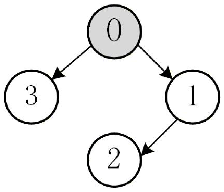
This section presents two examples to verify the effectiveness of the proposed distributed control scheme. The interaction topology among the agents is shown in Figure 2, in which node 0 represents the leader, and nodes 1–3 denote the followers.

4.1. Numerical Example

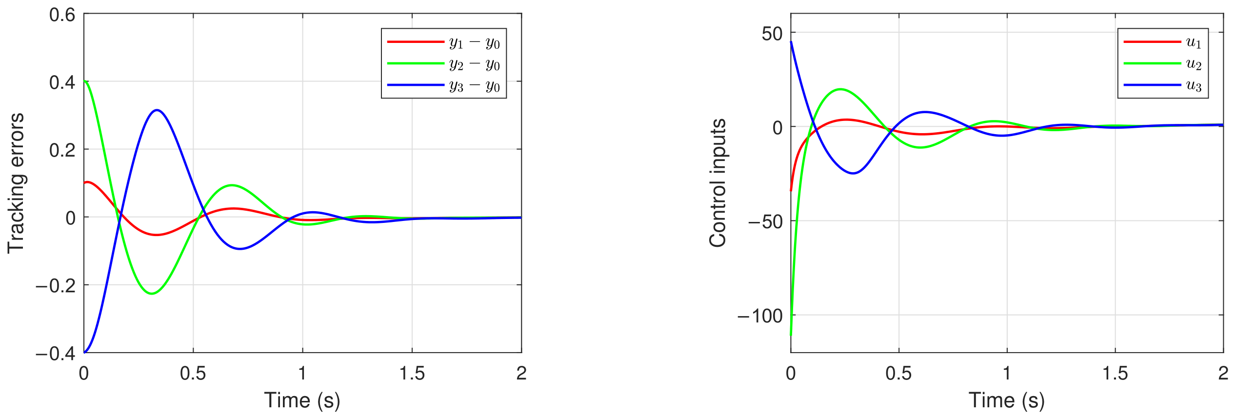
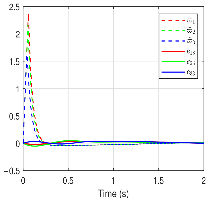
The i-th follower’s dynamics is given by (1), in which f 11 = 0.5 sin ( x 11 ) , f 12 = x 12 cos ( x 11 ) , f 21 = 0.3 sin ( x 21 ) , f 22 = x 22 cos ( x 21 ) , f 31 = x 31 sin ( x 32 ) , f 32 = x 32 cos ( x 31 ) , and d i = 2 cos ( t ) . The leader’s output is set to y 0 = 0.1 cos ( t ) . It is obvious that Assumptions 2 and 3 are satisfied. The follower’s initial states are taken as [ x 11 ( 0 ) , x 12 ( 0 ) ] = [ 0.2 , 0.3 ] , [ x 21 ( 0 ) , x 22 ( 0 ) ] = [ 0.5 , 0.1 ] , and [ x 31 ( 0 ) , x 32 ( 0 ) ] = [ 0.3 , 0.4 ] . The initial values for PTESO are set to zero. The design parameters are chosen as L = 8 , t 0 = 0 , t f = 2 , κ = 1.2 , [ b 11 , b 12 ] = [ 2 , 17.5 ] , [ b 21 , b 22 ] = [ 2 , 13 ] , [ b 31 , b 32 ] = [ 1.5 , 6.66 ] , [ k i 1 , k i 2 , k i 3 ] = [ 2.8 , 5.7 , 2.8 ] , ϵ i = 1 , and
P i = 1.2364 0.4506 0.0896 0.4506 0.5739 0.4577 0.0896 0.4577 0.6842 .
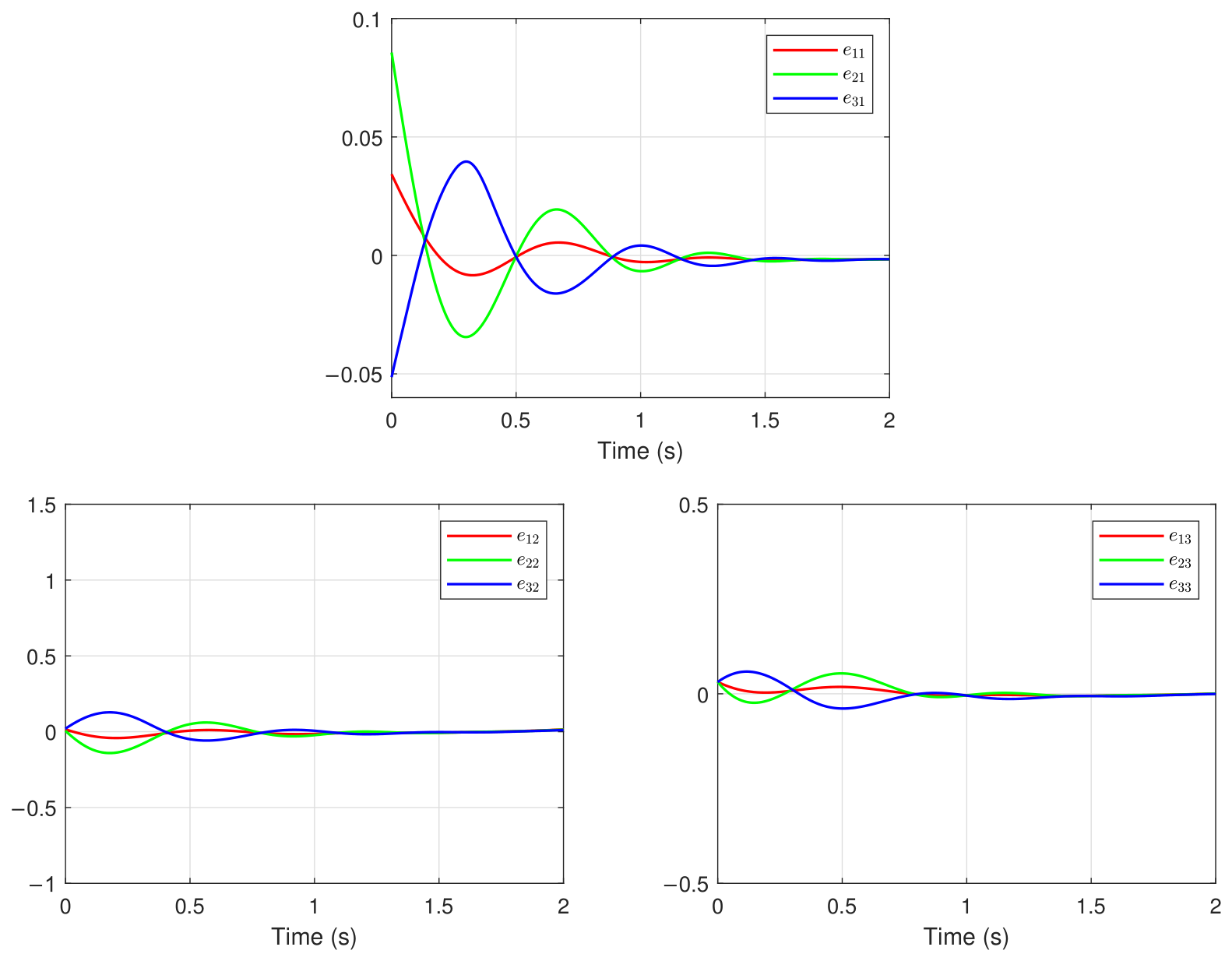
The simulation results are illustrated in Figure 3 and Figure 4. Figure 3 depicts the tracking errors and control inputs, from which it can be observed that the outputs y i of all followers achieve the precise tracking of the leader’s output y 0 within the prescribed time. The observation errors corresponding to z i 1 , z i 2 , and ω i are demonstrated in Figure 4. It is shown that the observation errors e i 1 , e i 2 and e i 3 converge to zero within the prescribed time interval.

4.2. Application Example

To further validate the effectiveness of the proposed method, it was applied to a servo-actuator-driven robotic manipulator system and compared with the observer-based fixed-time synchronization control method proposed in [16]. The dynamics of each robotic manipulator are described as follows:
J i θ ¨ i + B i θ ˙ i + M i g L i sin ( θ i ) = u m i + d m i ,
where θ i and θ ˙ i are the link position and velocity, respectively. u m i represents the torque input. M i and L i denote the link mass and length, respectively. B i is the damping coefficient; J i is the rotational inertia. In practical engineering applications, the physical implementation of the control input is inevitably affected by actuator non-idealities and external loads, resulting in a discrepancy between the actual joint torque applied to the manipulator and the ideal control input. This discrepancy can be equivalently regarded as an unknown disturbance d m i acting on the system.
Let x i , 1 = θ i , x i , 2 = θ ˙ i , then (73) becomes
x ˙ i , 1 = x i , 2 x ˙ i , 2 = ( B i / J i ) x i , 2 ( M i g L i / J i ) sin ( x i , 1 ) + u i + d i ,
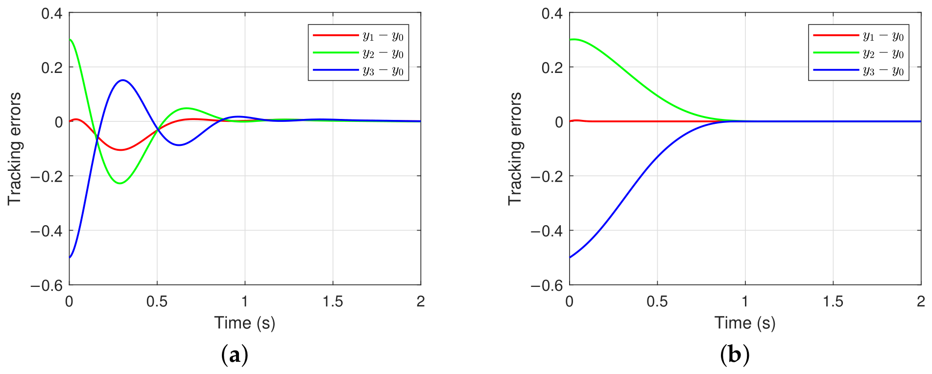
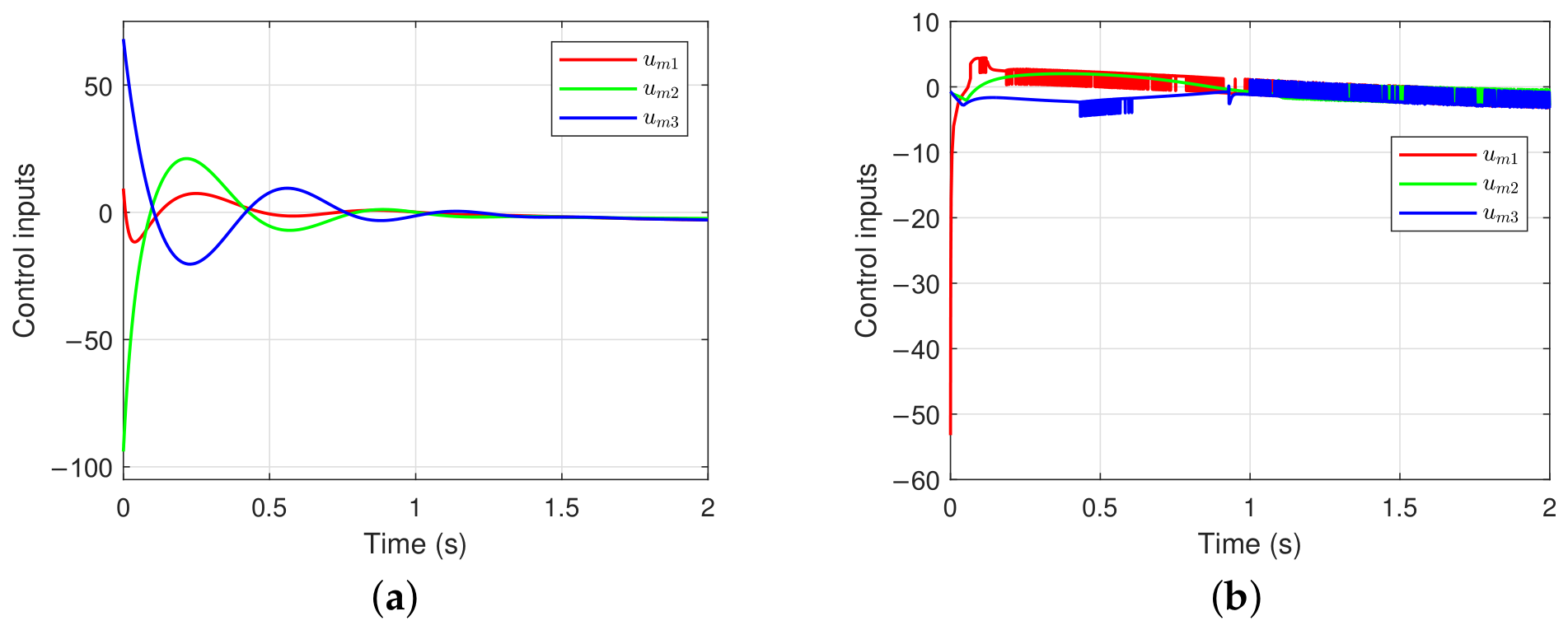
where u i = u m i / J i , d i = d m i / J i . The system parameters are selected as B 1 = B 2 = B 3 = 0.18 , J 1 = J 2 = J 3 = 1.1 , M 1 = M 3 = 1.3 , M 2 = 1 , L 1 = L 3 = 1.2 , L 2 = 0.8 , and g = 9.8 . The external disturbance is chosen as d m i = 2 sin ( t ) , and the leader’s output is given by y 0 = 0.2 cos ( t ) . The controller parameters and the initial conditions of the proposed method are the same as those in Section 4.1. The controller parameters of the method in [16] are selected according to the tuning procedure provided in the original paper. To ensure a fair comparison, both methods were implemented under the same simulation settings, including identical initial conditions, network topology, and external disturbances.
Figure 5, Figure 6 and Figure 7 compare the tracking errors, disturbance estimation errors, and control inputs of the two methods. As shown in Figure 5, both methods achieve satisfactory tracking performance. Figure 6 indicates that both methods provide satisfactory disturbance estimation performance, while the proposed method exhibits a smaller peak disturbance estimation error during the initial stage and a smoother estimation process than the method in [16]. Figure 7 further shows that, although both methods accomplish the control task, the proposed method generates more continuous control inputs with significantly reduced high-frequency chattering, thereby alleviating the adverse effects of frequent actuator switching.

5. Conclusions

This brief addressed the prescribed-time output-feedback consensus tracking problem for nonlinear MASs with mismatched uncertainties and external disturbances. By avoiding conventional state transformations, the proposed approach eliminates the restrictive differentiability assumptions commonly imposed on mismatched nonlinearities, thereby broadening the class of systems to which ADRC can be effectively applied. A PTESO was designed to estimate both unmeasured states and disturbances, which was then integrated with a backstepping-based distributed controller to form a feedforward–feedback composite consensus protocol. The stability analysis, grounded in the homogeneous domination technique and prescribed-time Lyapunov theory, demonstrates that both the tracking errors and observer estimation errors converge to zero within a preassigned time, despite the coupling between the observer and controller dynamics. The simulation results confirm the practical feasibility of the proposed scheme. Future research directions include extending the proposed framework to higher-order MASs with input saturation and exploring event-triggered communication strategies to further reduce network bandwidth consumption in resource-constrained environments.

Author Contributions

Conceptualization, X.S. and J.H.; methodology, X.S. and J.H.; validation, X.S.; investigation, X.S., J.H. and X.W.; writing—original draft preparation, X.S.; writing—review and editing, X.S., J.H. and X.W. All authors have read and agreed to the published version of this manuscript.

Funding

This work was supported in part by the National Key Research and Development Program of China under grant 2022YFE0133100 and in part by Sichuan Science and Technology Program under grant 2025YFHZ0134.

Institutional Review Board Statement

Not applicable.

Informed Consent Statement

Not applicable.

Data Availability Statement

The data used to support the findings of this study are available from the corresponding author upon request.

Conflicts of Interest

The authors declare no conflicts of interest.

References

  1. Shao, J.; Zhou, Q.; Ye, D.; Bernelli-Zazzera, F.; Sun, Z. Feasibility analysis and synchron ization control for underactuated spacecraft formationhovering. IEEE Trans. Control Syst. Technol. 2024, 32, 241–249. [Google Scholar] [CrossRef] [Scilit]
  2. Ye, H.; Wen, C.; Song, Y. Distributed matrix pencil formulations for prescribed-time leader-following consensus of MASs with unknown sensor sensitivity. IEEE Trans. Syst. Man Cybern. Syst. 2026, 56, 629–641. [Google Scholar] [CrossRef] [Scilit]
  3. Zhang, D.; Hu, J.; Cheng, J.; Wu, Z.-G.; Yan, H. A novel disturbance observer based fixed-time sliding mode control for robotic manipulators with global fast convergence. IEEE/CAA J. Autom. Sin. 2024, 11, 661–672. [Google Scholar] [CrossRef] [Scilit]
  4. Yoo, S.J. Distributed consensus tracking for multiple uncertain nonlinear strict-feedback systems under a directed graph. IEEE Trans. Neural Netw. Learn. Syst. 2013, 24, 666–672. [Google Scholar] [CrossRef] [Scilit] [PubMed]
  5. Zhang, X.; Liu, L.; Feng, G. Leader–follower consensus of time-varying nonlinear multi-agent systems. Automatica 2015, 52, 8–14. [Google Scholar] [CrossRef] [Scilit]
  6. Zhang, J.-X.; Yang, G.-H. Distributed fuzzy adaptive output feedback control of unknown nonlinear multiagent systems in strict feedback form. IEEE Trans. Cybern. 2022, 52, 5607–5617. [Google Scholar] [CrossRef] [Scilit] [PubMed]
  7. Shen, Q.; Shi, P. Distributed command filtered backstepping consensus tracking control of nonlinear multiple-agent systems in strict-feedback form. Automatica 2015, 53, 120–124. [Google Scholar] [CrossRef] [Scilit]
  8. Cao, L.; Pan, Y.; Liang, H.; Huang, T. Observer-based dynamic event triggered control for multiagent systems with time-varying delay. IEEE Trans. Cybern. 2023, 53, 3376–3387. [Google Scholar] [CrossRef] [Scilit] [PubMed]
  9. Katsoukis, I.; Rovithakis, G.A. A low complexity robust output synchronization protocol with prescribed performance for high-order heterogeneous uncertain MIMO nonlinear multiagent systems. IEEE Trans. Autom. Control 2022, 67, 3128–3133. [Google Scholar] [CrossRef] [Scilit]
  10. Wang, X.; Wang, H.; Huang, T.; Kurths, J. Neural-network based adaptive tracking control for nonlinear multiagent systems: The observer case. IEEE Trans. Cybern. 2023, 53, 138–150. [Google Scholar] [CrossRef] [Scilit] [PubMed]
  11. Sui, J.; Liu, C.; Niu, B.; Zhao, X.; Wang, D.; Yan, B. Prescribed performance adaptive containment control for full-state constrained nonlinear multiagent systems: A disturbance observer-based design strategy. IEEE Trans. Autom. Sci. Eng. 2025, 22, 179–190. [Google Scholar] [CrossRef] [Scilit]
  12. Zhang, Y.; Sun, J.; Liang, H.; Li, H. Event-triggered adaptive tracking control for multiagent systems with unknown disturbances. IEEE Trans. Cybern. 2020, 50, 890–901. [Google Scholar] [CrossRef] [Scilit] [PubMed]
  13. Jing, Y.H.; Yang, G.H. Fuzzy adaptive quantized fault-tolerant control of strict-feedback nonlinear systems with mismatched external disturbances. IEEE Trans. Syst. Man Cybern. Syst. 2020, 50, 3424–3434. [Google Scholar] [CrossRef] [Scilit]
  14. Zhu, F.; Zhao, Y.; Fu, Y.; Dinh, T.N. Observer-based output consensus control scheme for strict-feedback nonlinear multi-agent systems with disturbances. IEEE Trans. Netw. Sci. Eng. 2024, 11, 2621–2631. [Google Scholar] [CrossRef] [Scilit]
  15. Wang, Z.; Sheng, S. Finite time disturbance observer-based adaptive composite control for disturbed unmanned helicopter. ISA Trans. 2025, 163, 139–150. [Google Scholar] [CrossRef] [Scilit] [PubMed]
  16. Jin, X.; Jiang, J.; Qin, J.; Zheng, W.; Gao, M. Observer-based fixed-time-synchronized control for uncertain Euler–Lagrange systems with bias–actuator faults. IEEE Trans. Cybern. 2025, 55, 3811–3824. [Google Scholar] [CrossRef] [Scilit] [PubMed]
  17. Gao, M.; Ding, L.; Jin, X. Elm-based adaptive faster fixed-time control of robotic manipulator systems. IEEE Trans. Neural Netw. Learn. Syst. 2023, 34, 4646–4658. [Google Scholar] [CrossRef] [Scilit] [PubMed]
  18. Xiao, W.; Ren, H.; Zhou, Q.; Li, H.; Lu, R. Distributed finite-time containment control for nonlinear multiagent systems with mismatched disturbances. IEEE Trans. Cybern. 2022, 52, 6939–6948. [Google Scholar] [CrossRef] [Scilit] [PubMed]
  19. Shen, X.; Hu, J.; Xue, W.; Meng, B. Finite-time output consensus control of nonlinear uncertain multi-agent systems via extended state observer. Syst. Control Lett. 2024, 194, 105967. [Google Scholar] [CrossRef] [Scilit]
  20. Cao, L.; Cheng, Z.; Liu, Y.; Li, H. Event-based adaptive NN fixed-time cooperative formation for multiagent systems. IEEE Trans. Neural Netw. Learn. Syst. 2024, 35, 6467–6477. [Google Scholar] [CrossRef] [Scilit] [PubMed]
  21. Song, Y.; Ye, H.; Lewis, F.L. Prescribed-time control and its latest developments. IEEE Trans. Syst. Man Cybern. Syst. 2023, 53, 4102–4116. [Google Scholar] [CrossRef] [Scilit]
  22. Yang, S.; Liao, C.; Ji, L.; Jin, Q. Prescribed-time tracking control for uncertain nonlinear multiagent systems with matched and mismatched disturbances. IEEE Trans. Syst. Man Cybern. Syst. 2025, 55, 6100–6111. [Google Scholar] [CrossRef] [Scilit]
  23. Kim, H.J.; Yoo, S.J. Disturbance observer-based adaptive chainlike filter approach for prescribed-time consensus tracking of nonlinear multiagent systems via dynamic state and input triggering. IEEE Trans. Cybern. 2025, 55, 4001–4014. [Google Scholar] [CrossRef] [Scilit] [PubMed]
  24. Wang, Z.; Cao, Z.; Zhang, L.; Wang, H.; Xu, N. Active disturbance rejection predefined-time consensus tracking for nonlinear multiagent systems via self-triggered communication. IEEE Trans. Autom. Sci. Eng. 2024, 22, 9810–9820. [Google Scholar]
  25. Lv, J.; Wang, C.; Liu, B.; Kao, Y.; Jiang, Y. Predefined-time output-feedback leader-following consensus of pure-feedback multiagent systems. IEEE Trans. Cybern. 2024, 54, 7754–7766. [Google Scholar] [CrossRef] [Scilit] [PubMed]
  26. Shen, X.; Wu, Y.; Hu, J.; Zhou, Q. Prescribed-time active disturbance rejection control for nonlinear systems with mismatched uncertainties: A non-separation principle approach. IEEE Trans. Autom. Sci. Eng. 2025, 22, 22886–22899. [Google Scholar] [CrossRef] [Scilit]
  27. Zou, A.-M.; Liu, Y.; Hou, Z.-G.; Hu, Z. Practical predefined-time output-feedback consensus tracking control for multiagent systems. IEEE Trans. Cybern. 2023, 53, 5311–5322. [Google Scholar] [CrossRef] [Scilit] [PubMed]
  28. Lin, Y.; Dong, C.; Wang, Q. Practical prescribed-time output tracking control of uncertain nonaffine systems with input saturation based on time base generator. ISA Trans. 2025, 162, 111–118. [Google Scholar] [CrossRef] [Scilit] [PubMed]
  29. Bacciotti, A.; Roiser, L. Liapunov Functions and Stability in Control Theory, 2nd ed.; Springer: Berlin/Heidelberg, Germany, 2005. [Google Scholar]
  30. Hu, J.; Hong, Y. Leader-following coordination of multi-agent systems with coupling time delays. Phys. A Stat. Mech. Its Appl. 2007, 374, 853–863. [Google Scholar] [CrossRef] [Scilit]
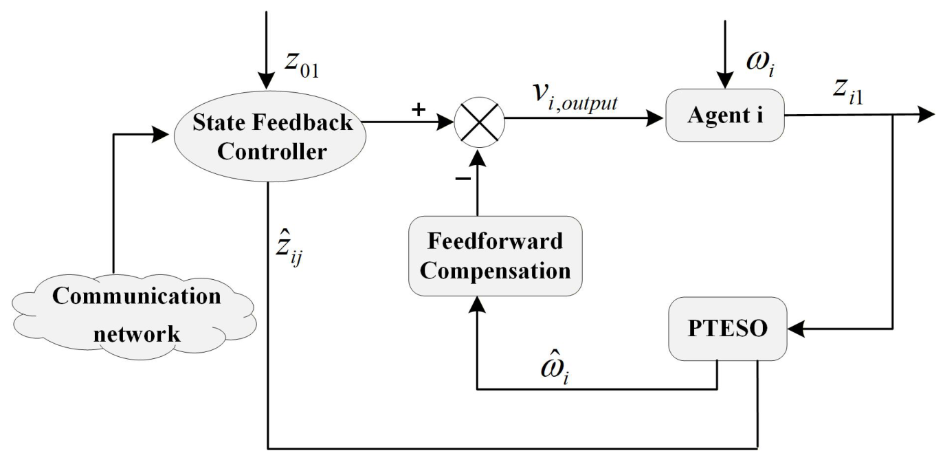
Figure 1. Block diagram of PTESO-based prescribed-time composite control strategy.
Actuators 15 00394 g001
Figure 2. The interaction topology.
Actuators 15 00394 g002
Figure 3. Tracking errors and control inputs.
Actuators 15 00394 g003
Figure 4. The observation errors for z i 1 , z i 2 and ω i .
Actuators 15 00394 g004
Figure 5. Tracking errors. (a) Proposed method. (b) Method in [16].
Actuators 15 00394 g005
Figure 6. Disturbance estimation errors. Dashed: method in [16]; Solid: proposed method.
Actuators 15 00394 g006
Figure 7. Control inputs. (a) Proposed method. (b) Method in [16].
Actuators 15 00394 g007
Disclaimer/Publisher’s Note: The statements, opinions and data contained in all publications are solely those of the individual author(s) and contributor(s) and not of MDPI and/or the editor(s). MDPI and/or the editor(s) disclaim responsibility for any injury to people or property resulting from any ideas, methods, instructions or products referred to in the content.