Adaptive Tracking Control of Nonstrict-Feedback Nonlinear Systems with Actuator Faults and Input Delay via a Fuzzy Funnel Approach

Abstract

This article investigates an adaptive fuzzy funnel control approach for nonstrict-feedback nonlinear systems with actuator faults and input delay. Fuzzy logic systems (FLSs) are utilized to estimate unknown functions, while the Pade approximation technique is applied to address the effects of input delay. By leveraging the approximation capabilities of FLSs and the backstepping control technique, an adaptive funnel control scheme is developed. This scheme ensures that all closed-loop signals are semi-globally uniformly ultimately bounded (SGUUB). Utilizing funnel control, the tracking error is kept within a predefined funnel and converges to a specified interval using a funnel function. The effectiveness of the proposed controller is validated with a real-world example involving an electromechanical system.

1. Introduction

In recent years, nonlinear control systems have found extensive applications in various fields such as manufacturing, defense, and aviation. Research in nonlinear control systems has emerged as a critical frontier, leading to significant advancements. However, the increasing complexity of modern nonlinear systems and the higher demands for control accuracy necessitate further study. Therefore, developing control theories and methods for nonlinear systems is of paramount importance [1,2,3,4]. The backstepping method is a widely used design approach for controlling nonlinear systems. It begins with the lowest order differential equation of the system. Through a step-by-step design process, virtual states and virtual controls are introduced. Ultimately, the real control law is formulated in the final step. In recent decades, considerable attention has been given to the control problems of nonlinear systems with uncertainties. Several significant control methods have been proposed to address various systems with these uncertainties [5,6,7]. Adaptive control is another crucial method for managing nonlinear systems. It excels in approximating unknown parameters and handling uncertain model structures. However, due to practical demands and theoretical challenges, numerous important studies have been conducted to handle the presence of unknown functions in actual systems. Fuzzy logic systems (FLSs) and neural networks (NNs), known for their ability to approximate functions universally, have been incorporated into adaptive control designs to address unknown functions, yielding many promising results [8,9,10]. For instance, a neural network-based adaptive scheme has been reported for nonlinear systems with state constraints on functions [11]. Additionally, an adaptive neural control scheme using approximate models has been introduced for nonlinear systems [12]. For nonlinear systems with state constraints, an adaptive fuzzy finite-time control scheme utilizing an observer has been published [13]. Furthermore, for nonstrict-feedback stochastic nonlinear systems, an adaptive fuzzy control scheme has been developed [14].

Actuators, as the executive components in control systems, play a crucial role in determining control performance. However, they are often subject to faults due to operating under high temperatures, high pressure, and other adverse conditions [15]. Identifying these faults promptly during actuator operation and taking appropriate measures are essential to ensure the safety and stability of automatic control systems. This has led to increased interest in fault-tolerant control (FTC) methods in recent years [16,17,18,19]. For example, an adaptive control approach utilizing neural networks has been developed for fractional-order nonlinear systems with actuator faults [20]. Additionally, a fuzzy control method has been proposed for managing nonlinear systems under actuator faults [21]. For nonlinear uncertain systems experiencing actuator faults, a neural network-based adaptive event-triggered control strategy has been introduced [22].

Time delay significantly impacts the control accuracy of systems, and it is an inevitable issue due to hardware limitations in actual systems. Addressing and mitigating the influence of time delay to enhance control performance has been a critical research area [23,24,25]. Recent improvements in time-delay systems have focused on enhancing delay-dependent analysis and stability requirements. Flexible fragmentation methods for passivity analysis [26] and generalized reciprocally convex inequality-based stability analysis [27] have given effective tools for delayed systems. These advancements further drive the exploration of nonlinear control systems with input delays. In practical systems, input delay is another common type of delay, especially in networked-feedback control systems, where traditional delay approaches are ineffective. To tackle this, adaptive control methods based on the Pade approximation technique have been developed for nonlinear systems. Over decades of intensive research, several effective methods for managing input delay have been proposed [28,29,30]. For example, a fuzzy adaptive control scheme has been introduced for nonlinear strict-feedback systems with input delay [31]. Additionally, a fuzzy finite-time adaptive control approach has been published for active suspension nonlinear systems experiencing input delay [32]. For nonlinear systems with input delay and state constraints, a neural adaptive control scheme has been reported [30]. Furthermore, for nonlinear multi-agent systems with input delay, a fuzzy observer adaptive finite-time control method has been developed [33].

In industrial applications, control systems often face challenges in ensuring both transient and steady-state performance. To tackle this problem, prescribed performance control was developed [34]. This approach guarantees the convergence rate and limits the maximum overshoot of the tracking error. It works by analytically evaluating and defining the desired performance during both transient and steady-state phases, using a prescribed performance function and a coordinate error transformation. However, calculating the partial differential for the transformation error can cause stability problems. Additionally, funnel control has been used to ensure a prescribed transient response, aiming to regulate transient behavior and confine the steady-state tracking error within a specified range. Without needing complex identification and estimation procedures, funnel control has been effectively applied to nonlinear systems. In recent years, numerous successful applications of funnel control in nonlinear systems have been reported [35,36,37]. For instance, a fuzzy adaptive funnel control approach has been developed for nonlinear systems with a dead-zone and saturation [38]. A fuzzy finite-time funnel adaptive control scheme has been published for nonaffine nonlinear systems [39]. Furthermore, for nonlinear systems with hysteresis input and unknown control coefficients, adaptive funnel control via dynamic surface control and observer has been reported [40]. An adaptive event-triggered platoon control strategy for heterogeneous vehicles was developed using a funnel-based predefined-time control framework in [41].

Recent breakthroughs in intelligent and nonlinear control have led to considerable improvements in the robustness and performance of complex engineering systems. Finite-time control for nonlinear UAV systems [42], distributed distributionally robust model predictive control [43], optimization-based UAV trajectory design [44], and reinforcement learning-based robust consensus control for heterogeneous multi-agent systems [45,46] have all shown encouraging results under practical constraints and uncertainties. Adaptive fuzzy funnel control for nonstrict-feedback nonlinear systems with actuator defects and input delay is not covered by these studies, despite the fact that they offer insightful information about intelligent and robust control. Motivated by these problems, this work presents an adaptive fuzzy funnel control technique to achieve excellent tracking performance and closed-loop stability.

This article is motivated by the ongoing difficulties in obtaining high-performance control of nonlinear systems operating under realistic constraints. Due to component deterioration, communication lags, and signal transmission delays, actuator problems and input delays frequently occur concurrently in a variety of engineering applications, including electromechanical systems, robotic manipulators, autonomous cars, and aerospace systems. If not appropriately addressed, the cohabitation of these elements might seriously impair tracking performance and possibly jeopardize system stability. The simultaneous treatment of actuator faults and input delays within a funnel control framework for nonstrict-feedback nonlinear systems has gotten very little attention, despite significant advancements in nonlinear control.This drives the creation of the suggested adaptive fuzzy funnel control approach, which attempts to improve the tracking performance, robustness, and dependability of nonlinear systems facing these real-world difficulties. This paper makes significant contributions compared to existing research:

• Compared with existing results [12,13,14], this paper focuses on addressing nonstrict-feedback nonlinear systems that face challenges like actuator faults and input delay simultaneously. To effectively handle input delay, the paper introduces the Pade approximation technique within a unified framework, making it applicable to a wider range of practical systems. Furthermore, a funnel variable is defined to overcome non-differentiable issues as in [47], ensuring that the output tracking error consistently remains within a predefined boundary.
• The paper proposes an adaptive controller based on the backstepping method and Lyapunov analysis. The proposed controller is designed to ensure that all signals within the closed-loop system are semiglobally uniformly ultimately bounded (SGUUB). It achieves this by adjusting specific design parameters, guaranteeing that the tracking error remains within a specified interval. The feasibility and efficacy of this control method are demonstrated through a simulated example.

The following is the format for the remainder of the paper: The problem statement and the essential preliminaries are introduced in Section 2. We review the controller design procedure and perform stability analysis in Section 3. Section 4 presents an illustrative example to demonstrate the efficacy of the proposed controller. Finally, the paper is concluded in Section 5.

Notation

In this article, $\mathbb{R}$ denotes the set of real numbers, and ${\mathbb{R}}^n$ represents the n-dimensional Euclidean space. The notation ${(·)}^T$ denotes the transpose of a vector. For a signal $x\left(t\right)$, $\left|x\right|$ denotes its absolute value, while $\parallel x\parallel$ denotes the Euclidean norm. $\eta ={[{\eta }_1,{\eta }_2,\dots ,{\eta }_n]}^T\in {\mathbb{R}}^n$ denotes the system state vector, where ${\eta }_i$$(i=1,2,\dots ,n)$ is the ith state. The functions ${\varphi }_i\left(\eta \right)$ represent unknown nonlinear functions satisfying ${\varphi }_i\left(0\right)=0$. The terms $p_i\left(t\right)$ denote bounded external disturbances satisfying $|p_i\left(t\right)|\le {\overline{p}}_i$, where ${\overline{p}}_i$ is a positive constant. The variable $v\left(t\right)$ is the control input, while $u\left(v\right(t-\tau \left)\right)$ denotes the actuator output in the presence of actuator faults and an input delay. The constant $\tau >0$ represents the input delay, and $y={\eta }_1$ is the system output.

2. Problem Statement and Preliminaries

Consider the nonlinear systems in nonstrict-feedback form as

$$\left\{\begin{array}{c}{\dot{\eta }}_i={\varphi }_i\left(\eta \right)+{\eta }_{i+1}+p_i\left(t\right), 1\le i\le n-1,\hfill \\ {\dot{\eta }}_n={\varphi }_n\left(\eta \right)+u\left(v(t-\tau )\right)+p_n\left(t\right),\hfill \\ y={\eta }_1,\hfill \end{array}\right.$$

(1)

with $\eta ={[{\eta }_1,\dots ,{\eta }_n]}^T$ being the state vector, ${\varphi }_i(·)$ being the nonlinear unknown functions with ${\varphi }_i\left(0\right)=0$, and $p_i\left(t\right)$ being the external disturbances with $|p_i\left(t\right)|\le {\overline{p}}_i$, where ${\overline{p}}_i$ is a constant. u is the system output subjected to input delay and actuator faults, $\tau$ indicates the input delay, and y is the system output.

To address the problem of input delay and obtain the real control law v, the Pade approximation, as described in [23], is used, which is defined as

$$\begin{array}{cc}\hfill L\left\{u\right(v(t-\kappa )\left)\right\}& =\exp (-\kappa s)L\left\{u\left(v\left(t\right)\right)\right\}\approx {\displaystyle \frac{1-\frac{\kappa s}{2}}{1+\frac{\tau s}{2}}}L\left\{u\left(v\left(t\right)\right)\right\},\hfill \end{array}$$

(2)

with $L\left\{u\right(v\left(t\right)\left)\right\}$ being the Laplace transform of $u\left(t\right)$ and s being the Laplace variable.

The new variable ${\eta }_{n+1}$ can be formulated as

$$L\left\{{\eta }_{n+1}\left(t\right)\right\}={\displaystyle \frac{1-\frac{\kappa s}{2}}{1+\frac{\kappa s}{2}}}L\left\{u\left(v\left(t\right)\right)\right\}+L\left\{u\left(v\left(t\right)\right)\right\}.$$

(3)

By putting $\rho ={\displaystyle \frac{2}{t_d}}$ and using inverse Laplace transform, we have

$${\dot{\eta }}_{n+1}={\displaystyle \frac{4}{\kappa }}u\left(v\left(t\right)\right)-{\displaystyle \frac{2}{\kappa }}{\eta }_{n+1}=2\rho u\left(v\left(t\right)\right)-\rho {\eta }_{n+1}.$$

(4)

From (2)–(4), (2) becomes

$$\left\{\begin{array}{c}{\dot{\eta }}_i={\varphi }_i\left({\eta }_i\right)+{\eta }_{i+1}+p_i\left(t\right), 1\le i\le n-1,\hfill \\ {\dot{\eta }}_n={\varphi }_n\left({\eta }_n\right)+{\eta }_{n+1}-u\left(v\left(t\right)\right)+p_n\left(t\right),\hfill \\ {\dot{\eta }}_{n+1}=-\rho {\eta }_{n+1}+2\rho u\left(v\left(t\right)\right),\hfill \\ y={\eta }_1,\hfill \end{array}\right.$$

(5)

with $u\left(v\right(t\left)\right)$ being the system inputs influenced by actuator faults which can be formulated as [48]

$$u\left(v\right(t\left)\right)=\gamma \left(t\right)v+\zeta \left(t\right),$$

(6)

where $\gamma \left(t\right)\in (0,1]$ represents the effectiveness factor of the actuator, v is the control input, and $\zeta \left(t\right)$ is the uncontrollable additive actuation fault.

From (6), the system (5) becomes

$$\left\{\begin{array}{c}{\dot{\eta }}_i={\varphi }_i\left({\eta }_i\right)+{\eta }_{i+1}+p_i\left(t\right), 1\le i\le n-1,\hfill \\ {\dot{\eta }}_n={\varphi }_n\left({\eta }_n\right)+{\eta }_{n+1}-\gamma \left(t\right)v-\zeta \left(t\right)+p_n\left(t\right),\hfill \\ {\dot{\eta }}_{n+1}=-\rho {\eta }_{n+1}+2\rho \gamma \left(t\right)v+2\rho \zeta \left(t\right),\hfill \\ y={\eta }_1,\hfill \end{array}\right.$$

(7)

Remark 1.

The variable ${\eta }_{n+1}$ is a recently introduced element designed to handle input delay effectively. It functions as an intermediate parameter rather than being regarded as a primary system state variable [23].

The main goal in control is to ensure that the tracking error $e_1=y\left(t\right)-y_d\left(t\right)$ remains within a predetermined range, referred to as a funnel. This funnel is mathematically defined as $F:=\{(t,e_1)\in {\mathbb{R}}^{+}\times \mathbb{R}\mid |e_1|<F_{\psi }\left(t\right)\}$, where the boundary of the funnel is denoted by $\partial F\left(t\right)=F_{\psi }\left(t\right)$. Essentially, for any given time $t>0$, we aim for $(t,e_1)$ to be part of the set F. The specific form of $F_{\psi }\left(t\right)$ is chosen as follows [38]

$$F_{\psi }\left(t\right)=({\beta }_0-{\beta }_{\infty })e^{-\alpha t}+{\beta }_{\infty }$$

(8)

where ${\beta }_0>0$, ${\beta }_{\infty }>0$, and $\alpha >0$ are design parameters; it is notable that ${\lim }_{t\to \infty }{F}_{\psi }={\beta }_{\infty }$.

In study [38], the authors introduced a funnel variable ${\xi }_1={\displaystyle \frac{e_1}{F_{\psi }^2-\left|e_1\right|}}$. However, it is observed that ${\xi }_1$ becomes non-differentiable at $e_1\left(t\right)=0$, which does not align with the controller design requirements based on backstepping.

To resolve the non-differentiability problem in [47], a funnel error transformation is introduced as

$${\xi }_1={\displaystyle \frac{e_1}{\sqrt{F_{\psi }^2-e_1^2}}}$$

(9)

with $e_1={\eta }_1-y_d$. The time-derivative of ${\xi }_1$ is expressed as

$${\dot{\xi }}_1={{\rm Y}}_1\left({\dot{\eta }}_1-{\dot{y}}_d-{\displaystyle \frac{e_1{\dot{F}}_{\psi }}{F_{\psi }}}\right)$$

(10)

where ${{\rm Y}}_1={\displaystyle \frac{F_{\psi }^2}{{(F_{\psi }^2-e_1^2)}^3}}$.

Remark 2.

It is noted that the proposed funnel transformation ${\xi }_1={\displaystyle \frac{e_1}{\sqrt{F_{\psi }^2-e_1^2}}}$ is well-defined under the condition $|e_1\left(t\right)|<F_{\psi }\left(t\right)$, which is guaranteed by the funnel constraint definition. Since $F_{\psi }\left(t\right)>0$ for all $t\ge 0$, the denominator satisfies $F_{\psi }^2\left(t\right)-e_1^2\left(t\right)>0$, $\forall t\ge 0$, which ensures that ${\xi }_1$ remains finite for all admissible trajectories. Furthermore, as long as the tracking error remains strictly inside the funnel boundary, the mapping $e_1\mapsto {\xi }_1$ is continuously differentiable with respect to time. In particular, both $e_1\left(t\right)$ and $F_{\psi }\left(t\right)$ are continuously differentiable functions, and the denominator never approaches zero. Hence, no singularity occurs as $e_1\left(t\right)$ approaches the funnel boundary, since the control design guarantees that $|e_1\left(t\right)|<F_{\psi }\left(t\right)$ is preserved for all $t\ge 0$. Therefore, the proposed funnel transformation is smooth ($C^1$) over the entire admissible funnel region and fully compatible with the backstepping-based adaptive control design.

The objective of the control approach is to create an adaptive fuzzy funnel tracking controller v for the system described in (1). This controller must ensure that all signals in the closed-loop system demonstrate SGUUB characteristics. Moreover, the controller should keep the tracking error within a defined funnel boundary.

Assumption 1

([24]). The reference signal $y_d\left(t\right)$ and its nth derivatives with respect to time are continuous and bounded.

Assumption 2

([48]). The functions $\gamma \left(t\right)$ and $\zeta \left(t\right)$ defined in (6) satisfy ${\gamma }_{\min }<\gamma \left(t\right)\le 1$ and $\left|\zeta \left(t\right)\right|\le {\zeta }_{\max }$, where ${\gamma }_{\min }>0$ and ${\zeta }_{\max }>0$ are constants.

Remark 3.

Assumption 1 ensures that the reference signal $y_d\left(t\right)$ and its time derivatives $y_d^{\left(n\right)}\left(t\right)$ remain bounded, guaranteeing the boundedness of all variables throughout the backstepping procedure. This assumption is commonly employed in the design of adaptive controllers, as supported by various studies, including references [25,28,49]. Assumption 2 states that the control gain $\gamma \left(t\right)$ and the unknown additive actuator fault $\zeta \left(t\right)$ are not predetermined. Therefore, the conventional stability criterion cannot be applied [48].

Lemma 1

([50]). For all $(a,b)\in {\mathbb{R}}^2$, $ϵ>0$, one has

$$ab\le {\displaystyle \frac{{ϵ}^c}{c}}{\left|a\right|}^c+{\displaystyle \frac{1}{d{ϵ}^c}}{\left|b\right|}^d,$$

(11)

where $c>1$, $d>1$, and $(c-1)(d-1)=1$.

Fuzzy logic systems [21]: A fuzzy logic system can be created by following these steps to approximate a continuous function $\varphi \left(X\right)$ specified on a compact set $\Omega$. The following is how we define a collection of If–Then fuzzy rules:

$$R^l:\mathrm{If} {\eta }_1 \mathrm{is} F_1^l \mathrm{and} \dots \mathrm{and} {\eta }_n \mathrm{is} F_n^l, \mathrm{then} y \mathrm{is} G^l, l=1,2,\dots ,g,$$

(12)

where the input vector is $X={[{\eta }_1,\dots ,{\eta }_n]}^T$ and the fuzzy system’s output is y. The membership functions ${\mu }_{F_j^l}\left({\eta }_j\right)$ and ${\mu }_{G^l}\left(y\right)$ are connected to the fuzzy sets $F_j^l$ and $G^l$, respectively, where g represents the number of rules.

The fuzzy system’s output can be written as

$$y\left(X\right)={\displaystyle \frac{{\sum }_{l=1}^g{W}_l{\prod }_{j=1}^n{\mu }_{F_j^l}\left({\eta }_j\right)}{{\sum }_{l=1}^g{\prod }_{j=1}^n{\mu }_{F_j^l}\left({\eta }_j\right)}},$$

(13)

where $W_l={\max }_{y\in \mathbb{R}}{\mu }_{G^l}\left(y\right)$. We also define the fuzzy basis function as

$$S_l\left(X\right)={\displaystyle \frac{{\prod }_{j=1}^n{\mu }_{F_j^l}\left({\eta }_j\right)}{{\sum }_{l=1}^g{\prod }_{j=1}^n{\mu }_{F_j^l}\left({\eta }_j\right)}},$$

(14)

which enables the fuzzy logic system to be designed as

$$y\left(X\right)=W^{T}P\left(X\right),$$

(15)

where $\theta ={[{\theta }_1,{\theta }_2,\dots ,{\theta }_g]}^T$ and $P\left(X\right)={[P_1\left(X\right),P_2\left(X\right),\dots ,P_g\left(X\right)]}^T$.

Lemma 2

([21]). Consider a continuous function $\varphi \left(X\right)$ defined on a compact set Ω. There is a fuzzy logic system that, for any constant $ϵ>0$, can be presented as

$$\underset{X\in \Omega }{\sup }\left|\varphi \left(X\right)-{\theta }^{T}P\left(X\right)\right|\le ϵ.$$

(16)

3. Controller Design and Stability Analysis

This section focuses on using the backstepping method to create an adaptive fuzzy funnel controller. We start by implementing a coordinate transformation into practice as

$$\begin{array}{cc}\hfill z_1& ={\xi }_1 \hfill \end{array}$$

(17)

$$\begin{array}{cc}\hfill z_i& ={\eta }_i-{\alpha }_{i-1}, i=2,\dots ,n\hfill \end{array}$$

(18)

where the virtual control signal that needs to be designed is denoted by ${\alpha }_{i-1}$.

Step 1: The Lyapunov function is considered as

$$V_1={\displaystyle \frac{1}{2}}{\xi }_1^2+ {\displaystyle \frac{1}{2{\varsigma }_1}}{\tilde{\omega }}_1^2$$

(19)

where ${\tilde{\theta }}_1={\omega }_1-{\widehat{\omega }}_1$ denotes the approximation error with ${\widehat{\omega }}_1$ being the estimation of ${\omega }_1$, defined as ${\omega }_1={\parallel {\theta }_1^{\ast }\parallel }^2$, and ${\varsigma }_1$ is a design positive parameter.

The derivative of $V_1$ produces

$$\begin{array}{ccc}\hfill {\dot{V}}_1& =\hfill & \hfill {\xi }_1\left({{\rm Y}}_1{z}_2+{{\rm Y}}_1{\alpha }_1+{\overline{\varphi }}_1\right)-{\displaystyle \frac{1}{{\varsigma }_1}}{\tilde{\omega }}_1{\dot{\widehat{\omega }}}_1,\end{array}$$

(20)

where ${\overline{\varphi }}_1={{\rm Y}}_1\left({\varphi }_1-{\dot{y}}_d-{\displaystyle \frac{e_1{\dot{F}}_{\psi }}{F_{\psi }}}\right)$.

Lemma 1 indicates that the fuzzy logic system ${\theta }_1^{\ast T}{P}_1\left(X_1\right)$ is applied to approximate the unknown function ${\overline{\varphi }}_1$, ensuring that for any specified ${ϵ}_1>0$

$${\overline{\varphi }}_1\left(X_1\right)={\theta }_1^{\ast T}{P}_1\left(X_1\right)+{\delta }_1\left(X_1\right), \left|{\delta }_1\left(X_1\right)\right|\le {ϵ}_1,$$

(21)

where $X_1={[{\eta }_1,\dots ,{\eta }_n]}^T$, and ${\delta }_1\left(X_1\right)$ represents the estimation error.

Through the use of Lemmas 1 and 2, it is established that

$$\begin{array}{cc}\hfill {\xi }_1{\overline{f}}_1\left(X_1\right)& ={\xi }_1\left({\theta }_1^{\ast T}{P}_1\left(X_1\right)+{\delta }_1\left(X_1\right)\right)\hfill \\ \hfill & \le |{\xi }_1|\left(\parallel {\theta }_1^{\ast }\parallel \parallel P_1\left(X_1\right)\parallel +{ϵ}_1\right)\hfill \\ \hfill & \le |{\xi }_1|\left(\parallel {\theta }_1^{\ast }\parallel \parallel P_1\left(Z_1\right)\parallel +{ϵ}_1\right)\hfill \\ \hfill & \le {\displaystyle \frac{1}{2a_1^2}}{\xi }_1^2{\omega }_1{P}_1^T\left(Z_1\right)P_1\left(Z_1\right)+{\displaystyle \frac{a_1^2}{2}}+{\displaystyle \frac{{\xi }_1^2}{2}}+{\displaystyle \frac{{ϵ}_1^2}{2}},\hfill \end{array}$$

(22)

where ${\omega }_1={\parallel {\theta }_1^{\ast }\parallel }^2$, $Z_1={\left[{\eta }_1\right]}^T$, and $a_1>0$ is a constant.

Utilizing Lemma 1, it is evident that

$${\xi }_1{p}_1\left(t\right)\le {\displaystyle \frac{{\xi }_1^2}{2}}+{\displaystyle \frac{{\overline{p}}_1^2}{2}},$$

(23)

with ${\overline{p}}_1>0$ being a constant.

The formulation of the virtual controller ${\alpha }_1$ can be represented as

$$\begin{array}{cc}\hfill {\alpha }_1& =-{\displaystyle \frac{1}{{\Gamma }_1}}\left(k_1{\xi }_1+{\displaystyle \frac{1}{2}}{\xi }_1+{\displaystyle \frac{1}{2a_1^2}}{\xi }_1{\widehat{\omega }}_1{P}_1^T\left(Z_1\right)P_1\left(Z_1\right)\right),\hfill \end{array}$$

(24)

where $k_1>0$ and $a_1>0$ represent the design parameters.

Using Lemma 1 along with (24), we have

$$\begin{array}{cc}\hfill {\xi }_1{\alpha }_1& \le -{\displaystyle \frac{1}{{{\rm Y}}_1}}\left(k_1{\xi }_1^2+{\displaystyle \frac{1}{2a_1^2}}{\xi }_1^2{\widehat{\omega }}_1{P}_1^T\left(Z_1\right)P_1\left(Z_1\right)\right),\hfill \end{array}$$

(25)

Substituting (22)–(25) into (20), we have

$$\begin{array}{cc}\hfill {\dot{V}}_1& \le -k_1{\xi }_1^2+\left({\displaystyle \frac{1}{2a_1^2}}{\xi }_1^2{P}_1^T\left(Z_1\right)P_1\left(Z_1\right)\right)({\omega }_1-{\widehat{\omega }}_1)+{\displaystyle \frac{{\overline{p}}_1^2}{2}}+{\displaystyle \frac{a_1^2}{2}}+{\displaystyle \frac{{\xi }_1^2}{2}}+{\displaystyle \frac{{ϵ}_1^2}{2}}-{\displaystyle \frac{1}{{\varsigma }_1}}{\tilde{\omega }}_1{\dot{\widehat{\omega }}}_1\hfill \end{array}$$

(26)

Given that ${\tilde{\omega }}_1={\omega }_1-{\widehat{\omega }}_1$, we can rewrite (26) as

$$\begin{array}{cc}\hfill {\dot{V}}_1& \le -k_1{\xi }_1^2+{\displaystyle \frac{{\overline{p}}_1^2}{2}}+{\displaystyle \frac{a_1^2}{2}}+{\displaystyle \frac{{\xi }_1^2}{2}}+{\displaystyle \frac{{ϵ}_1^2}{2}}+{\displaystyle \frac{1}{{\varsigma }_1}}{\tilde{\omega }}_1\left({\displaystyle \frac{1}{2a_1^2}}{\varsigma }_1{\xi }_1^2{P}_1^T\left(Z_1\right)P_1\left(Z_1\right)-{\dot{\widehat{\omega }}}_1\right)\hfill \end{array}$$

(27)

The adaptive law ${\dot{\widehat{\omega }}}_1$ is expressed as

$$\begin{array}{cc}\hfill {\dot{\widehat{\omega }}}_1& ={\displaystyle \frac{{\varsigma }_1}{2a_1^2}}{z}_1^2{P}_1^T\left(Z_1\right)P_1\left(Z_1\right)-{\vartheta }_1{\widehat{\omega }}_1, {\widehat{\omega }}_1\left(0\right)\ge 0,\hfill \end{array}$$

(28)

with ${\varsigma }_1$ and $a_1$ being the design positive parameters.

By inserting (28) into (27), one obtains

$${\dot{V}}_1\le -k_1^2{\chi }_1^2+{\rm Y}{\chi }_1{z}_2+{\displaystyle \frac{1}{{\varsigma }_1}}{\vartheta }_1{\tilde{\omega }}_1{\widehat{\omega }}_1+{\displaystyle \frac{a_1}{2}}+{\displaystyle \frac{{ϵ}_1^2}{2}}+{\displaystyle \frac{{\overline{p}}_1^2}{2}}.$$

(29)

Step i ($2\le n-1$): By utilizing (17) and (7), one has

$${\dot{z}}_i={\dot{\eta }}_i-{\dot{\alpha }}_{i-1}={\varphi }_i\left(\eta \right)+{\eta }_{i+1}+p_i\left(t\right)-{\dot{\alpha }}_{i-1}.$$

(30)

with

$${\dot{\alpha }}_{i-1}={\displaystyle \sum _{j=0}^{i-1}}{\displaystyle \frac{\mathsf{\partial }{\alpha }_{i-1}}{\mathsf{\partial }{y}_d^{\left(j\right)}}}{y}_r^{(j+1)}+{\displaystyle \sum _{j=1}^{i-1}}{\displaystyle \frac{\mathsf{\partial }{\alpha }_{i-1}}{\mathsf{\partial }{\eta }_j}}({\varphi }_j\left(\eta \right)+{\eta }_{j+1}+p_j\left(t\right))+{\displaystyle \sum _{j=1}^{i-1}}{\displaystyle \frac{\mathsf{\partial }{\alpha }_{i-1}}{\mathsf{\partial }{\omega }_j}}{\dot{\omega }}_j.$$

(31)

Choose the Lyapunov function as

$$V_i=V_{i-1}+{\displaystyle \frac{1}{2}}{z}_i^2+{\displaystyle \frac{1}{2{\varsigma }_i}}{\tilde{\omega }}_i^2,$$

(32)

where ${\tilde{\omega }}_i={\omega }_i-{\widehat{\omega }}_i$, and ${\varsigma }_i$ is a positive design constant.

The derivative of $V_i$ produces

$$\begin{array}{cc}\hfill {\dot{V}}_i& \le {\dot{V}}_{i-1}+z_i({\varphi }_i\left(\eta \right)+z_{i+1}+{\alpha }_i+p_i\left(t\right)-{\dot{\alpha }}_{i-1})-{\displaystyle \frac{1}{{\varsigma }_i}}{\tilde{\omega }}_i{\dot{\widehat{\omega }}}_i.\hfill \end{array}$$

(33)

From (29), one has

$${\dot{V}}_{i-1}\le -{\displaystyle \sum _{j=1}^{i-1}}{k}_j{\xi }_j^2+z_{i-1}{z}_i+{\displaystyle \sum _{j=1}^{i-1}}{\displaystyle \frac{1}{{\varsigma }_j}}{\vartheta }_j{\tilde{\omega }}_j{\widehat{\omega }}_j+{\displaystyle \sum _{j=1}^{i-1}}\left({\displaystyle \frac{a_j^2}{2}}+{\displaystyle \frac{{ϵ}_j^2}{2}}+{\displaystyle \frac{{\overline{p}}_j^2}{2}}\right)$$

(34)

Upon substituting (34) into (35), we obtain

$$\begin{array}{cc}\hfill {\dot{V}}_i& \le -k_1{\xi }_1^2-{\displaystyle \sum _{j=2}^{i-1}}+z_{i-1}{z}_i+{\displaystyle \sum _{j=1}^{i-1}}{\displaystyle \frac{1}{{\varsigma }_j}}{\delta }_j{\tilde{\omega }}_j{\widehat{\omega }}_j+{\displaystyle \sum _{j=1}^{i-1}}\left({\displaystyle \frac{a_j^2}{2}}+{\displaystyle \frac{{ϵ}_j^2}{2}}+{\displaystyle \frac{{\overline{d}}_j^2}{2}}\right)\hfill \\ & +z_i({\overline{\varphi }}_i\left(X_i\right)+z_{i+1}+p_i\left(t\right)+{\alpha }_i)-{\displaystyle \frac{1}{{\varsigma }_i}}{\tilde{\omega }}_i{\dot{\widehat{\omega }}}_i-{\displaystyle \frac{1}{2}}{z}_i^2,\hfill \end{array}$$

(35)

where ${\overline{\varphi }}_i\left(X_i\right)={\varphi }_i\left(x\right)-{\dot{\alpha }}_{i-1}+{\displaystyle \frac{1}{2}}{z}_i$.

Lemma 2 indicates that the fuzzy logic system ${\theta }_i^{\ast T}{P}_i\left(X_i\right)$ is applied to approximate the unknown function ${\overline{\varphi }}_i$, such that for any specified ${ϵ}_i>0$

$${\overline{\varphi }}_i\left(X_i\right)={\theta }_i^{\ast T}{P}_i\left(X_i\right)+{\delta }_i\left(X_i\right), \left|{\delta }_i\left(X_i\right)\right|<{\epsilon }_i,$$

(36)

where $X_i={[{\eta }_1,\dots ,{\eta }_n,{\widehat{\omega }}_1,\dots ,{\widehat{\omega }}_{i-1}]}^T$.

By employing a method similar to that in (22), we have

$$z_i{\overline{\varphi }}_i\le {\displaystyle \frac{1}{2a_i^2}}{z}_i^2{\omega }_i{P}_i^T\left(Z_i\right)P_i\left(Z_i\right)+{\displaystyle \frac{a_i^2}{2}}+{\displaystyle \frac{z_i^2}{2}}+{\displaystyle \frac{{ϵ}_i^2}{2}},$$

(37)

where $Z_i={[{\eta }_1,\dots ,{\eta }_i,{\widehat{\omega }}_1,\dots ,{\widehat{\omega }}_{i-1}]}^T$, ${\omega }_i={\parallel {\theta }_i^{\ast }\parallel }^2$, and $a_i$ is a positive design parameter.

Utilizing Lemma 1, we have

$$z_i{p}_i\left(t\right)\le {\displaystyle \frac{z_i^2}{2}}+{\displaystyle \frac{{\overline{p}}_i^2}{2}},$$

(38)

with ${\overline{p}}_i$ being a positive constant.

The formulation for the virtual controller ${\alpha }_i$ is given as

$$\begin{array}{cc}\hfill {\alpha }_i& =-k_i{z}_i-z_{i-1}-{\displaystyle \frac{1}{2a_i^2}}{z}_i{\widehat{\omega }}_i{P}_i^T\left(Z_i\right)P_i\left(Z_i\right),\hfill \end{array}$$

(39)

with $k_i$ and $a_i$ being the design positive constants.

One can derive from Lemma 1 and (39) that

$$\begin{array}{cc}\hfill z_i{\alpha }_i& \le =-k_i{z}_i^2-z_i{z}_{i-1}-{\displaystyle \frac{1}{2a_i^2}}{z}_i^2{\widehat{\omega }}_i{P}_i^T\left(Z_i\right)P_i\left(Z_i\right),\hfill \end{array}$$

(40)

Substituting (37)–(40) into (35), one has

$$\begin{array}{cc}\hfill {\dot{V}}_i& \le -k_1{\xi }_1^2-{\displaystyle \sum _{j=2}^i}{k}_j{z}_j^2+{\displaystyle \sum _{j=1}^{i-1}}{\displaystyle \frac{1}{{\varsigma }_j}}{\vartheta }_j{\tilde{\omega }}_j{\widehat{\omega }}_j+{\displaystyle \sum _{j=1}^i}\left({\displaystyle \frac{a_j^2}{2}}+{\displaystyle \frac{{ϵ}_j^2}{2}}+{\displaystyle \frac{{\overline{p}}_j^2}{2}}\right)\hfill \\ \hfill & +\left({\displaystyle \frac{1}{2a_i^2}}{z}_i^2{P}_i^T\left(Z_i\right)P_i\left(Z_i\right)\right)({\omega }_i-{\widehat{\omega }}_i)-{\displaystyle \frac{1}{{\varsigma }_i}}{\tilde{\omega }}_i{\dot{\widehat{\omega }}}_i\hfill \end{array}$$

(41)

Since ${\tilde{\omega }}_i={\omega }_i-{\widehat{\omega }}_i$, (3.25) produces

$$\begin{array}{cc}\hfill {\dot{V}}_i& \le -k_1{\xi }_1^2-{\displaystyle \sum _{j=2}^i}{k}_j{z}_j^2+{\displaystyle \sum _{j=1}^{i-1}}{\displaystyle \frac{1}{{\varsigma }_j}}{\vartheta }_j{\tilde{\omega }}_j{\widehat{\omega }}_j+{\displaystyle \sum _{j=1}^i}\left({\displaystyle \frac{a_j^2}{2}}+{\displaystyle \frac{{ϵ}_j^2}{2}}+{\displaystyle \frac{{\overline{p}}_j^2}{2}}\right)\hfill \\ \hfill & +{\displaystyle \frac{1}{{\varsigma }_1}}{\tilde{\omega }}_i\left({\displaystyle \frac{1}{2a_i^2}}{\varsigma }_i{z}_i^2{P}_i^T\left(Z_i\right)P_i\left(Z_i\right)-{\dot{\widehat{\omega }}}_i\right)\hfill \end{array}$$

(42)

The formulation for the adaptive law ${\dot{\widehat{\omega }}}_i$ is given as

$$\begin{array}{cc}\hfill {\dot{\widehat{\omega }}}_i& ={\displaystyle \frac{{\varsigma }_i}{2a_i^2}}{z}_i^2{S}_i^T\left(Z_i\right)S_i\left(Z_i\right)-{\vartheta }_i{\widehat{\omega }}_i,\hfill \end{array}$$

(43)

where ${\varsigma }_i$ and ${\vartheta }_i$ stand for the design positive constants.

Substituting (43) into (42), one has

$$\begin{array}{cc}\hfill {\dot{V}}_i& \le -k_1{\xi }_1^2{\displaystyle \sum _{j=2}^i}{k}_j{z}_j^2+{\displaystyle \sum _{j=1}^i}{\displaystyle \frac{1}{{\varsigma }_j}}{\vartheta }_j{\tilde{\omega }}_j{\widehat{\omega }}_j+{\displaystyle \sum _{j=1}^i}\left({\displaystyle \frac{a_j^2}{2}}+{\displaystyle \frac{{ϵ}_j^2}{2}}+{\displaystyle \frac{{\overline{p}}_j^2}{2}}\right).\hfill \end{array}$$

(44)

Step n: The time derivative of $z_n$ according to (17) and (7) is given as

$${\dot{z}}_n={\dot{x}}_n-{\dot{\alpha }}_{n-1}={\varphi }_n\left(\eta \right)+{\eta }_{n+1}-\gamma \left(t\right)v-\zeta \left(t\right)+p_n\left(t\right)-{\dot{\alpha }}_{n-1}+{\displaystyle \frac{{\dot{\eta }}_{n+1}}{\rho }},$$

(45)

where the formulation of ${\alpha }_{n-1}$ can be expressed as

$${\dot{\alpha }}_{n-1}={\displaystyle \sum _{j=0}^{n-1}}{\displaystyle \frac{\partial {\alpha }_{n-1}}{\partial y_d^{\left(j\right)}}}{y}_r^{(j+1)}+{\displaystyle \sum _{j=1}^{n-1}}{\displaystyle \frac{\partial {\alpha }_{n-1}}{\partial x_j}}(f_j\left(x\right)+x_{j+1}+d_j\left(t\right))+{\displaystyle \sum _{j=1}^{n-1}}{\displaystyle \frac{\partial {\alpha }_{n-1}}{\partial {\omega }_j}}{\dot{\omega }}_j.$$

(46)

The Lyapunov function can be expressed as

$$V_n=V_{n-1}+{\displaystyle \frac{1}{2}}{z}_n^2+{\displaystyle \frac{1}{2{\varsigma }_n}}{\tilde{\omega }}_n^2,$$

(47)

with ${\tilde{\omega }}_n={\omega }_n-{\widehat{\omega }}_n$, and ${\varsigma }_n$ as the design positive constant.

The derivative of $V_n$ is formulated as

$$\begin{array}{cc}\hfill {\dot{V}}_n& \le {\dot{V}}_{n-1}+z_n({\varphi }_n\left(\eta \right)+{\eta }_{n+1}-\gamma \left(t\right)v-\zeta \left(t\right)+p_n\left(t\right)-{\dot{\alpha }}_{n-1}+{\displaystyle \frac{-\rho {\eta }_{n+1}}{\rho }}\hfill \\ \hfill & +{\displaystyle \frac{2\rho \gamma \left(t\right)v}{\rho }}+{\displaystyle \frac{2\rho \zeta \left(t\right)}{\rho }})-{\displaystyle \frac{1}{{\varsigma }_n}}{\tilde{\omega }}_n{\dot{\widehat{\omega }}}_n\hfill \\ \hfill & \le {\dot{V}}_{n-1}+z_n({\varphi }_n\left(\eta \right)+{\eta }_{n+1}-\gamma \left(t\right)v-\zeta \left(t\right)+p_n\left(t\right)-{\dot{\alpha }}_{n-1}-et{a}_{n+1}\hfill \\ \hfill & +2\gamma \left(t\right)v+2\zeta \left(t\right))-{\displaystyle \frac{1}{{\varsigma }_n}}{\tilde{\omega }}_n{\dot{\widehat{\omega }}}_n\hfill \\ \hfill & \le {\dot{V}}_{n-1}+z_n\left({\varphi }_n\left(\eta \right)+\gamma \left(t\right)v+\zeta \left(t\right)+p_n\left(t\right)-{\dot{\alpha }}_{n-1}\right)-{\displaystyle \frac{1}{{\varsigma }_n}}{\tilde{\omega }}_n{\dot{\widehat{\omega }}}_n.\hfill \end{array}$$

(48)

with

$${\dot{V}}_{n-1}\le -k_1{\xi }_1^2-{\displaystyle \sum _{j=2}^{n-1}}{k}_j{z}_j^2+{\displaystyle \sum _{j=1}^{n-1}}{\displaystyle \frac{1}{{\varsigma }_j}}{\vartheta }_j{\tilde{\omega }}_j{\widehat{\omega }}_j+{\displaystyle \sum _{j=1}^{n-1}}\left({\displaystyle \frac{a_j^2}{2}}+{\displaystyle \frac{{ϵ}_j^2}{2}}+{\displaystyle \frac{{\overline{p}}_j^2}{2}}\right).$$

(49)

By inserting (49) into (48), we obtain

$$\begin{array}{cc}\hfill {\dot{V}}_n& \le -k_1{\xi }_1^2-{\displaystyle \sum _{j=2}^{n-1}}{k}_j{z}_j^2+{\displaystyle \sum _{j=1}^{n-1}}{\displaystyle \frac{1}{{\varsigma }_j}}{\delta }_j{\tilde{\omega }}_j{\widehat{\omega }}_j+{\displaystyle \sum _{j=1}^{n-1}}\left({\displaystyle \frac{a_j^2}{2}}+{\displaystyle \frac{{ϵ}_j^2}{2}}+{\displaystyle \frac{{\overline{p}}_j^2}{2}}\right)\hfill \\ & +z_n\left({\overline{\varphi }}_n\left(X_n\right)+\gamma \left(t\right)v+\zeta \left(t\right)+p_n\left(t\right)\right)-{\displaystyle \frac{1}{{\varsigma }_n}}{\tilde{\omega }}_n{\dot{\widehat{\omega }}}_n-{\displaystyle \frac{1}{2}}{z}_n^2,\hfill \end{array}$$

(50)

where ${\overline{\varphi }}_n\left(X_n\right)={\varphi }_n\left(\eta \right)-{\dot{\alpha }}_{n-1}+{\displaystyle \frac{1}{2}}{z}_n$.

Lemma 1 indicates that the fuzzy logic system ${\theta }_n^{\ast T}{P}_n\left(X_n\right)$ is applied to approximate the unknown function ${\overline{\varphi }}_n$, such that for any specified ${ϵ}_n>0$

$${\overline{\varphi }}_n\left(X_n\right)={\theta }_n^T{P}_n\left(X_n\right)+{\delta }_n\left(X_n\right), \left|{\delta }_n\left(X_n\right)\right|<{\epsilon }_n,$$

(51)

where $X_n={[{\eta }_1,\dots ,{\eta }_n,{\widehat{\omega }}_1,\dots ,{\widehat{\omega }}_{n-1}]}^T$.

By employing a similar method as described in (22), one obtains

$$z_n{\overline{\varphi }}_n\le {\displaystyle \frac{1}{2a_n^2}}{z}_n^2{\omega }_n{P}_n^T\left(Z_n\right)P_n\left(Z_n\right)+{\displaystyle \frac{a_n^2}{2}}+{\displaystyle \frac{z_n^2}{2}}+{\displaystyle \frac{{ϵ}_n^2}{2}},$$

(52)

where $Z_n={[{\eta }_1,\dots ,{\eta }_n,{\widehat{\omega }}_1,\dots ,{\widehat{\omega }}_{n-1}]}^T$, ${\omega }_n={\parallel {\theta }_n^{\ast }\parallel }^2$, and $a_n>0$ represents the design parameter.

By utilizing Lemma 1, we have

$$z_n{p}_n\left(t\right)\le {\displaystyle \frac{z_n^2}{2}}+{\displaystyle \frac{{\overline{p}}_n^2}{2}},$$

(53)

with ${\overline{p}}_n$ being a positive constant.

By employing Lemma 1 alongside Assumption 2, one has

$$z_n\zeta \left(t\right)\le {\displaystyle \frac{z_n^2}{2}}+{\displaystyle \frac{{\zeta }_{\max }^2}{2}}.$$

(54)

The formulation of real controller v is given as

$$\begin{array}{cc}\hfill v& =-k_n{z}_n-z_{n-1}-{\displaystyle \frac{1}{2a_n^2}}{z}_n{\widehat{\omega }}_n{P}_n^T\left(Z_n\right)P_n\left(Z_n\right),\hfill \end{array}$$

(55)

with $k_n$ and $a_n$ being the positive constants.

Applying Assumption 2, Lemma 1, and (55) leads to

$$\begin{array}{cc}\hfill z_{n}v& \le =-k_n{\gamma }_{\min }{z}_n^2-z_n{z}_{n-1}-{\displaystyle \frac{1}{2a_n^2}}{z}_n^2{\widehat{\omega }}_n{P}_n^T\left(Z_n\right)P_n\left(Z_n\right).\hfill \end{array}$$

(56)

Substituting (52)–(56) into (50), one obtains

$$\begin{array}{cc}\hfill {\dot{V}}_i& \le -k_1{\xi }_1^2-{\displaystyle \sum _{j=2}^{n-1}}{k}_j{z}_j^2-k_n{\gamma }_{\min }{z}_n^2+{\displaystyle \sum _{j=1}^{i-1}}{\displaystyle \frac{1}{{\varsigma }_j}}{\vartheta }_j{\tilde{\omega }}_j{\widehat{\omega }}_j+{\displaystyle \sum _{j=1}^i}\left({\displaystyle \frac{a_j^2}{2}}+{\displaystyle \frac{{ϵ}_j^2}{2}}+{\displaystyle \frac{{\overline{p}}_j^2}{2}}\right)+{\displaystyle \frac{{\zeta }_{\max }^2}{2}}\hfill \\ \hfill & +\left({\displaystyle \frac{1}{2a_n^2}}{z}_n^2{P}_n^T\left(Z_n\right)P_n\left(Z_n\right)\right)({\omega }_n-{\widehat{\omega }}_n)-{\displaystyle \frac{1}{{\varsigma }_n}}{\tilde{\omega }}_i{\dot{\widehat{\omega }}}_n\hfill \end{array}$$

(57)

Since ${\tilde{\omega }}_n={\omega }_n-{\widehat{\omega }}_n$, (57) produces

$$\begin{array}{cc}\hfill {\dot{V}}_n& \le -k_1{\xi }_1^2-{\displaystyle \sum _{j=2}^{n-1}}{k}_j{z}_j^2-k_n{\gamma }_{\min }{z}_n^2+{\displaystyle \sum _{j=1}^{n-1}}{\displaystyle \frac{1}{{\varsigma }_j}}{\vartheta }_j{\tilde{\omega }}_j{\widehat{\omega }}_j+{\displaystyle \sum _{j=1}^n}\left({\displaystyle \frac{a_j^2}{2}}+{\displaystyle \frac{{ϵ}_j^2}{2}}+{\displaystyle \frac{{\overline{p}}_j^2}{2}}\right)+{\displaystyle \frac{{\zeta }_{\max }^2}{2}}\hfill \\ \hfill & +{\displaystyle \frac{1}{{\varsigma }_n}}{\tilde{\omega }}_n\left({\displaystyle \frac{1}{2a_n^2}}{\varsigma }_n{z}_n^2{P}_n^T\left(Z_n\right)P_n\left(Z_n\right)-{\dot{\widehat{\omega }}}_n\right).\hfill \end{array}$$

(58)

The formulation of the adaptive law ${\dot{\widehat{\omega }}}_n$ is given as

$$\begin{array}{cc}\hfill {\dot{\widehat{\omega }}}_n& ={\displaystyle \frac{{\varsigma }_n}{2a_n^2}}{z}_n^2{P}_n^T\left(Z_n\right)P_n\left(Z_n\right)-{\vartheta }_n{\widehat{\omega }}_n,\hfill \end{array}$$

(59)

where ${\varsigma }_n$ and ${\vartheta }_n$ are the positive constants.

By substituting (59) into (58) and incorporating Assumption 2, we have

$$\begin{array}{cc}\hfill {\dot{V}}_n& \le -k_n{\xi }_n^2-{\displaystyle \sum _{j=2}^{n-1}}{k}_j{z}_j^2-k_n{\gamma }_{\min }{z}_n^2+{\displaystyle \sum _{j=1}^n}{\displaystyle \frac{1}{{\varsigma }_j}}{\vartheta }_j{\tilde{\omega }}_j{\widehat{\omega }}_j+{\displaystyle \sum _{j=1}^n}\left({\displaystyle \frac{a_j^2}{2}}+{\displaystyle \frac{{ϵ}_j^2}{2}}+{\displaystyle \frac{{\overline{p}}_j^2}{2}}\right)+{\displaystyle \frac{{\gamma }_{\max }^2}{2}}.\hfill \end{array}$$

(60)

Theorem 1.

Considering the system (1) along with Assumptions 1 and 2, the proposed control strategy, including the virtual control signals as described in (24) and (39), the real control signal as given in (55), and the adaptive laws as given in (28), (43), and (59), ensures that all signals within the closed-loop system exhibit SGUUB behavior with $|e_1\left(0\right)|<|F_{\psi }\left(0\right)|$, and it guarantees that the tracking error remains within a specified funnel and has the capability to converge to a predetermined boundary.

Proof. 

Since

$${\tilde{\omega }}_j{\widehat{\omega }}_j\le {\omega }_j^2-{\tilde{\omega }}_j^2.$$

(61)

by inserting (61) into (60), we have

$$\begin{array}{cc}\hfill {\dot{V}}_n& \le -k_1{\xi }_1^2-{\displaystyle \sum _{j=2}^{n-1}}{k}_j{z}_j^2+k_n{\gamma }_{\min }{z}_n^2+{\displaystyle \sum _{j=1}^n}{\displaystyle \frac{1}{{\varsigma }_j}}{\vartheta }_j{\omega }_j^2-{\displaystyle \sum _{j=1}^n}{\displaystyle \frac{1}{{\varsigma }_j}}{\vartheta }_j{\tilde{\omega }}_j^2+{\displaystyle \sum _{j=1}^n}\left({\displaystyle \frac{a_j^2}{2}}+{\displaystyle \frac{{ϵ}_j^2}{2}}+{\displaystyle \frac{{\overline{p}}_j^2}{2}}\right)+{\displaystyle \frac{{\zeta }_{\max }^2}{2}}\hfill \\ \hfill & =-{\displaystyle \sum _{j=1}^{n-1}}{k}_j{z}_j^2+k_n{\gamma }_{\min }{z}_n^2-{\displaystyle \sum _{j=1}^n}{\displaystyle \frac{1}{{\varsigma }_j}}{\vartheta }_j{\tilde{\omega }}_j^2+{\displaystyle \sum _{j=1}^n}\left({\displaystyle \frac{1}{{\varsigma }_j}}{\vartheta }_j{\omega }_j^2+{\displaystyle \frac{a_j^2}{2}}+{\displaystyle \frac{{ϵ}_j^2}{2}}+{\displaystyle \frac{{\overline{p}}_j^2}{2}}\right)+{\displaystyle \frac{{\zeta }_{\max }^2}{2}}\hfill \\ \hfill & \le -c_0\left({\displaystyle \frac{1}{2}}{\xi }_2^2+{\displaystyle \sum _{j=2}^n}{\displaystyle \frac{1}{2}}{z}_j^2+{\displaystyle \sum _{j=1}^n}{\displaystyle \frac{1}{2{\varsigma }_j}}{\tilde{\omega }}_j^2\right)+d_0\hfill \\ \hfill & \le -c_0{V}_n+d_0,\hfill \end{array}$$

(62)

with $c_0=2m$, $m=\min \{k_1,\dots ,k_n{\gamma }_{\min },{\vartheta }_1,\dots ,{\vartheta }_n\}$, and $d_0={\sum }_{j=1}^n\left({\displaystyle \frac{{\vartheta }_j{\omega }_j^2}{{\varsigma }_j}}+{\displaystyle \frac{a_j^2}{2}}+{\displaystyle \frac{{ϵ}_j^2}{2}}+{\displaystyle \frac{{\overline{p}}_j^2}{2}}\right)+{\displaystyle \frac{{\zeta }_{\max }^2}{2}}$. From (62), we have

$$0\le V_n\le \left(V\left(0\right)-{\displaystyle \frac{d_0}{c_0}}\right)e^{-c_{0}t}+{\displaystyle \frac{d_0}{c_0}},$$

(63)

which means that all signals within the closed-loop system are SGUUB and $V\left(t\right)$ is bounded by ${\displaystyle \frac{d_0}{c_0}}$.

Additionally, from (63), we obtain

$${\displaystyle \frac{1}{2}}{\xi }_1^2\le \left(V\left(0\right)-{\displaystyle \frac{d_0}{c_0}}\right)e^{-c_{0}t}+{\displaystyle \frac{d_0}{c_0}}\le V\left(0\right)e^{-c_{0}t}+{\displaystyle \frac{d_0}{c_0}}.$$

(64)

By substituting (9) into (64), we obtain

$${\displaystyle \frac{e_1^2}{F_{\psi }^2-e_1^2}}\le 2V\left(0\right)+2{\displaystyle \frac{d_0}{c_0}},$$

(65)

which leads to

$$e_1^2\left(1+2V\left(0\right)+2{\displaystyle \frac{d_0}{c_0}}\right)\le \left(2V\left(0\right)+2{\displaystyle \frac{d_0}{c_0}}\right)F_{\psi }^2.$$

(66)

Furthermore, we have

$$|e_1|\le \sqrt{{\displaystyle \frac{2V\left(0\right)+2\frac{d_0}{c_0}}{1+2V\left(0\right)+2\frac{d_0}{c_0}}}}|F_{\psi }|<|F_{\psi }|,$$

(67)

which indicates that with precise adjustment of the design parameters, it is possible to minimize tracking errors within the specified boundary. □

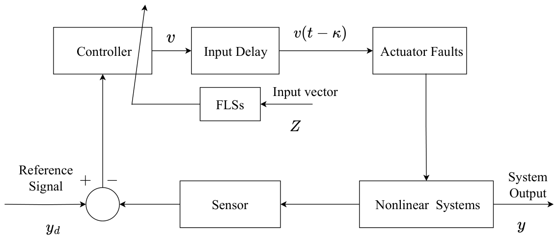
The diagram of the proposed control method is shown in Figure 1.

Remark 4.

The choice of design parameters has a significant impact on the controller’s performance; thus, choosing them wisely is essential. The tracking error tends to decrease as the parameters $k_i$ and ${\vartheta }_i$ are increased and $b_i$ is decreased. On the other hand, choosing extremely high values for $k_i$ and ${\vartheta }_i$ may lead to a higher control energy usage. Usually, a trial-and-error methodology is used to set both the beginning conditions and the design parameters. The system performance is then assessed and changes are made as necessary.

Remark 5.

In the Lyapunov-based stability analysis, the ultimate boundedness of the closed-loop system is affected by several sources of uncertainty, including fuzzy approximation errors, actuator faults, external disturbances, and input delay. Specifically, the fuzzy logic system approximation error satisfies $|{\delta }_1\left(X_1\right)|\le {ϵ}_1$, where ${ϵ}_1>0$ is a known constant. The actuator fault signals are bounded according to Assumption 2, where ${\gamma }_{\min }<\gamma \left(t\right)\le 1$ and $\left|\zeta \left(t\right)\right|\le {\zeta }_{\max }$, with ${\gamma }_{\min },{\zeta }_{\max }>0$. The external disturbances satisfy $|p_i\left(t\right)|\le {\overline{p}}_i$, where ${\overline{p}}_i$ are known positive constants. In addition, the input delay is constant and is handled via the Padé approximation, resulting in a bounded approximation error. Consequently, all uncertainty terms are uniformly bounded and appear additively in the Lyapunov derivative. Therefore, the final SGUUB bound depends explicitly on ${ϵ}_1$, ${\zeta }_{\max }$, ${\overline{p}}_i$, and the Padé approximation error. This shows that each source of uncertainty contributes in a quantifiable manner to the ultimate bound, and reducing these bounds or selecting appropriate controller gains can directly reduce the size of the ultimate tracking error set.

Remark 6.

The actuator effectiveness factor $\gamma \left(t\right)$ satisfies ${\gamma }_{\min }<\gamma \left(t\right)\le 1$, where ${\gamma }_{\min }>0$. As $\gamma \left(t\right)$ approaches its lower bound ${\gamma }_{\min }$, the control input remains well-defined and bounded due to the positivity of ${\gamma }_{\min }$. In this case, the proposed adaptive control law is still capable of compensating the reduced control authority, and the closed-loop system preserves SGUUB stability. However, a degradation in tracking performance may occur, reflected in a larger ultimate bound, when the actuator effectiveness decreases significantly.

Remark 7.

The input-delay system is converted into an enhanced delay-free representation using the Padé approximation. Although this approximation includes a modeling error, it remains confined for a constant input delay τ. This approximation mistake is regarded as an additional disturbance factor in the Lyapunov stability analysis. As a result, it makes an additive contribution to the closed-loop system’s final boundedness. As a result, the ultimate tracking performance is affected within a restricted range that is dictated by the Padé approximation error, but the SGUUB stability is maintained.

Remark 8.

The first-order Padé approximation is utilized to translate the input-delay system into an equivalent augmented delay-free model, hence enabling the adaptive backstepping controller design. Higher-order Padé approximations raise the system order, computational complexity, and difficulty of the relevant Lyapunov stability analysis, even though they may offer a more realistic depiction of the delayed dynamics. Therefore, the first-order Padé approximation is used as a compromise between approximation accuracy and implementation complexity. Furthermore, the approximation error introduced by the first-order Padé approximation stays confined for a constant input delay and is considered as extra uncertainty in the stability analysis. Consequently, the suggested controller preserves the SGUUB feature while maintaining adequate tracking performance with a very basic control structure.

Remark 9.

The proposed controller combines various fuzzy logic systems and adaptive parameter update rules to correct for unknown nonlinearities, actuator defects, and input delay. The online computations primarily incorporate fuzzy basis function evaluations, algebraic operations, and first-order adaptive parameter update rules, despite the fact that these components increase the computational overhead as compared to conventional controllers. Real-time implementation does not require matrix inversion or iterative optimization. The suggested control method is therefore computationally efficient and appropriate for implementation on contemporary embedded control platforms with enough processing power since the computational complexity increases roughly linearly with the number of fuzzy rules and system states.

4. Simulation Results

In this section, a practical example featuring an electromechanical system is provided to demonstrate the effectiveness of the presented control strategy.

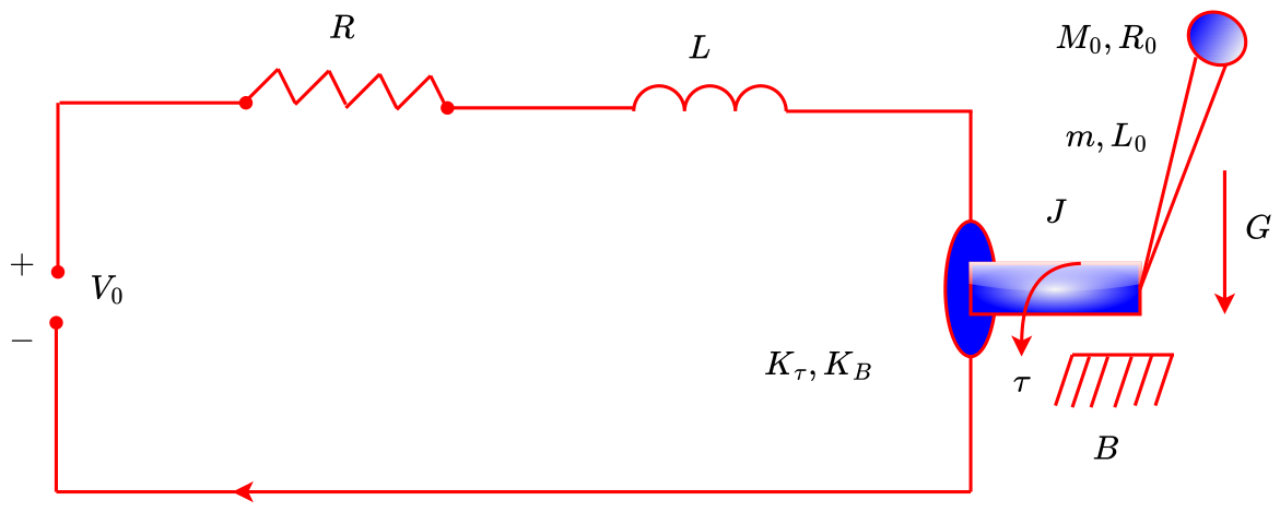
Example 1.

Consider the electromechanical system depicted in Figure 2 as presented in [51]:

$$\left\{\begin{array}{c}M\ddot{q}+B\dot{q}+N\sin \left(q\right)=\tau \hfill \\ L\dot{I}=V_0-RI-K_{\tau }\dot{q}\hfill \end{array}\right.$$

(68)

To simplify the analysis, we introduce variable changes as ${\eta }_1=q$, ${\eta }_2=\dot{q}$, ${\eta }_3=\tau$, and $u\left(v\right(t-\kappa \left)\right)=V$. This transforms the system’s dynamic model into the form

$$\left\{\begin{array}{c}{\dot{\eta }}_1={\eta }_2+f_1\left(\eta \right)+p_1\left(t\right)\hfill \\ {\dot{\eta }}_2={\eta }_3+f_2\left(\eta \right)+p_2\left(t\right)\hfill \\ {\dot{\eta }}_3=u\left(v(t-\kappa )\right)+f_3\left(\eta \right)+p_3\left(t\right)\hfill \\ y={\eta }_1\hfill \end{array}\right.$$

(69)

where $f_1\left(\eta \right)={\eta }_1^2\sin \left({\eta }_2{\eta }_3\right)$, $f_2\left(\eta \right)=-{\displaystyle \frac{N}{M}}\sin {\eta }_1-{\displaystyle \frac{B}{M}}{\eta }_2+{\displaystyle \frac{B}{M}}\cos {\eta }_2\sin {\eta }_3$, $f_3\left(\eta \right)=-{\displaystyle \frac{K}{L}}-{\displaystyle \frac{R}{L}}{\eta }_3$, $p_1\left(t\right)=0.2\cos \left(t\right)$, $p_2\left(t\right)=\cos \left(0.5t\right)$, $p_3\left(t\right)=0.2\sin \left(t\right)$, and $\kappa =1.5$ s. The system parameters and their values can be found in the existing work [51]. The reference trajectory is given as $y_d\left(t\right)=\sin \left(t\right)$.

The actuator fault model is formulated as

$$u\left(v\right)=\left\{\begin{array}{cc}v\hfill & \mathrm{if} t<10\hfill \\ (0.4+0.6\exp (-0.2t))v+{\cos }^2\left(x_1\right)x_2\hfill & \mathrm{if} t\ge 10\hfill \end{array}\right.$$

(70)

$\gamma \left(t\right)=0.4+0.6\exp (-0.2t)$, and $\zeta \left(t\right)={\cos }^2\left(x_1\right)x_2$.

The funnel function is formulated as

$$F_{\psi }\left(t\right)=(3-0.15)e^{-0.3t}+0.15,$$

(71)

where ${\beta }_0=3$, ${\beta }_{\infty }=0.15$, and $\alpha =0.3$.

We define fuzzy sets for each state variable within the interval $[-2,2]$, choosing specific partitioning points at $-2$, $-1.5$, $-0.5$, $0.5$, $1.5$, and 2. The membership functions for these fuzzy sets are formulated as follows ${\mu }_{F_j^1}\left(X\right)=\exp \left(-{\displaystyle \frac{{(X+2)}^2}{2}}\right)$, ${\mu }_{F_j^2}\left(X\right)=\exp \left(-{\displaystyle \frac{{(X+1.5)}^2}{2}}\right)$, ${\mu }_{F_j^3}\left(X\right)=\exp \left(-{\displaystyle \frac{{(X+0.5)}^2}{2}}\right)$, ${\mu }_{F_j^4}\left(X\right)=\exp \left(-{\displaystyle \frac{{(X-0.5)}^2}{2}}\right)$, ${\mu }_{F_j^5}\left(X\right)=\exp \left(-{\displaystyle \frac{{(X-1.5)}^2}{2}}\right)$, and ${\mu }_{F_j^6}\left(X\right)=\exp \left(-{\displaystyle \frac{{(X-2)}^2}{2}}\right)$. The virtual control ${\alpha }_1$, $alph{a}_2$, real control input v, and the adaptive laws ${\dot{\widehat{\omega }}}_i$ are constructed as

$$\begin{array}{cc}\hfill {\alpha }_1& =-{\displaystyle \frac{1}{{{\rm Y}}_1}}\left(-k_1{\xi }_1+{\displaystyle \frac{1}{2}}{\xi }_1-{\displaystyle \frac{1}{2a_i^2}}{e}_i{\widehat{\omega }}_i{S}_i^T\left(Z_i\right)S_i\left(Z_i\right)\right),\hfill \\ \hfill {\alpha }_2& =-k_2{z}_2-z_1-{\displaystyle \frac{1}{2a_2^2}}{z}_2{\widehat{\omega }}_2{S}_2^T\left(Z_2\right)S_2\left(Z_2\right),\hfill \\ \hfill v& =-k_3{z}_3-z_2-{\displaystyle \frac{1}{2a_3^2}}{z}_3{\widehat{\omega }}_3{S}_3^T\left(Z_3\right)S_3\left(Z_3\right),\hfill \\ \hfill {\dot{\widehat{\omega }}}_i& ={\displaystyle \frac{{\varsigma }_i}{2a_i^2}}{z}_i^2{S}_i^T\left(Z_i\right)S_i\left(Z_i\right)-{\vartheta }_i{\widehat{\omega }}_i, i=1,2,3.\hfill \end{array}$$

(72)

The controller parameters are chosen through a trial-and-error process as $k_1=4$, $k_2=4$, $k_3=6$, ${\vartheta }_1=1$, ${\vartheta }_2=1$, ${\vartheta }_3=1$, $a_1=a_2=a_3=2$, ${\varsigma }_1=1$, ${\varsigma }_2=1$, ${\varsigma }_3=1$. The initial conditions for the simulation are set through trial-and-error as ${[{\eta }_1\left(0\right),{\eta }_2\left(0\right),{\eta }_3\left(0\right)]}^T={[0.5,0.5,0.5]}^T$ and ${[{\widehat{\omega }}_1\left(0\right),{\widehat{\omega }}_2\left(0\right),{\widehat{\omega }}_3\left(0\right)]}^T={[0,0,0]}^T$.

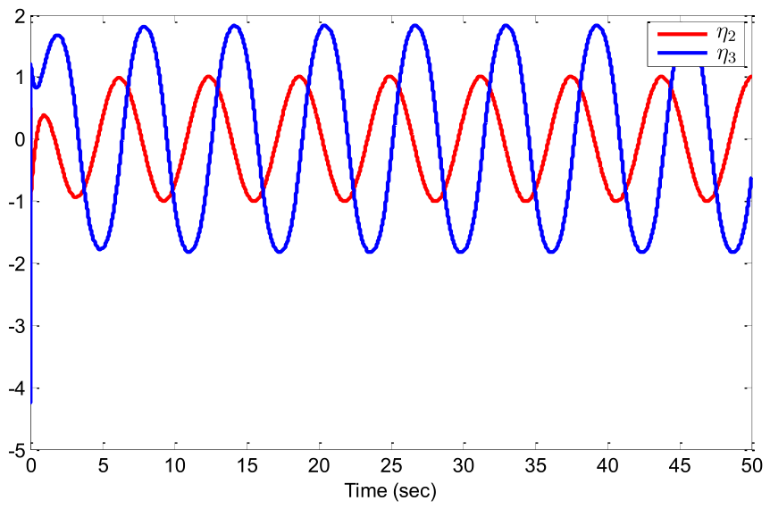
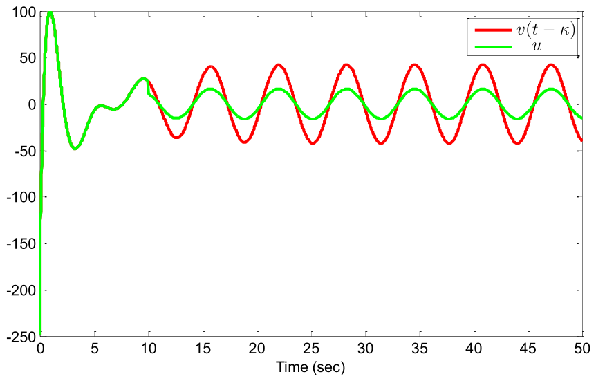
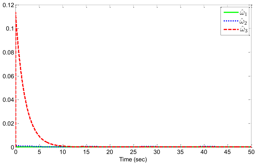
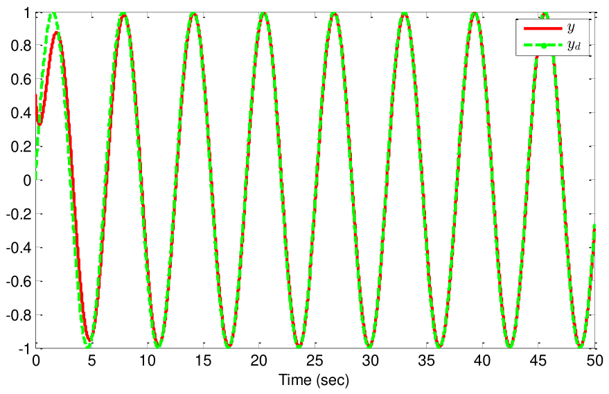
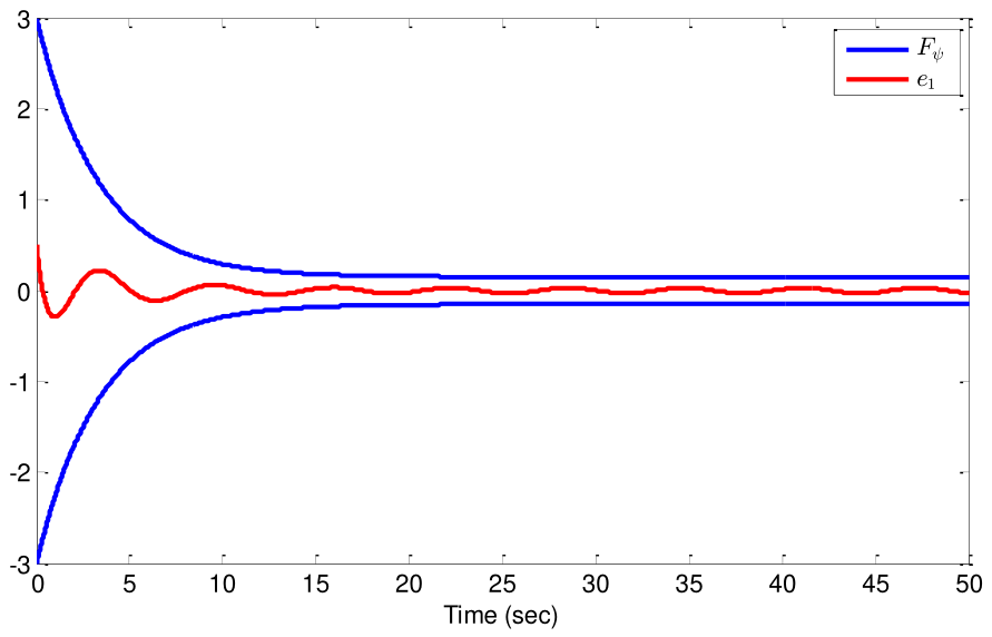
The results from the simulation are depicted in Figure 3, Figure 4, Figure 5, Figure 6, Figure 7 and Figure 8. Figure 3 illustrates the system output y alongside the reference signal $y_d$, showcasing successful tracking. The tracking error curve, as demonstrated in Figure 4, remains within the predefined funnel boundary. Figure 5 exhibits the input signals v and u. Additionally, Figure 6 and Figure 7 display the state variables ${\eta }_2$ and ${\eta }_3$, as well as the curves of the adaptive laws ${\widehat{\omega }}_1$, ${\widehat{\omega }}_2$, and ${\widehat{\omega }}_3$, all demonstrating bounded behavior.

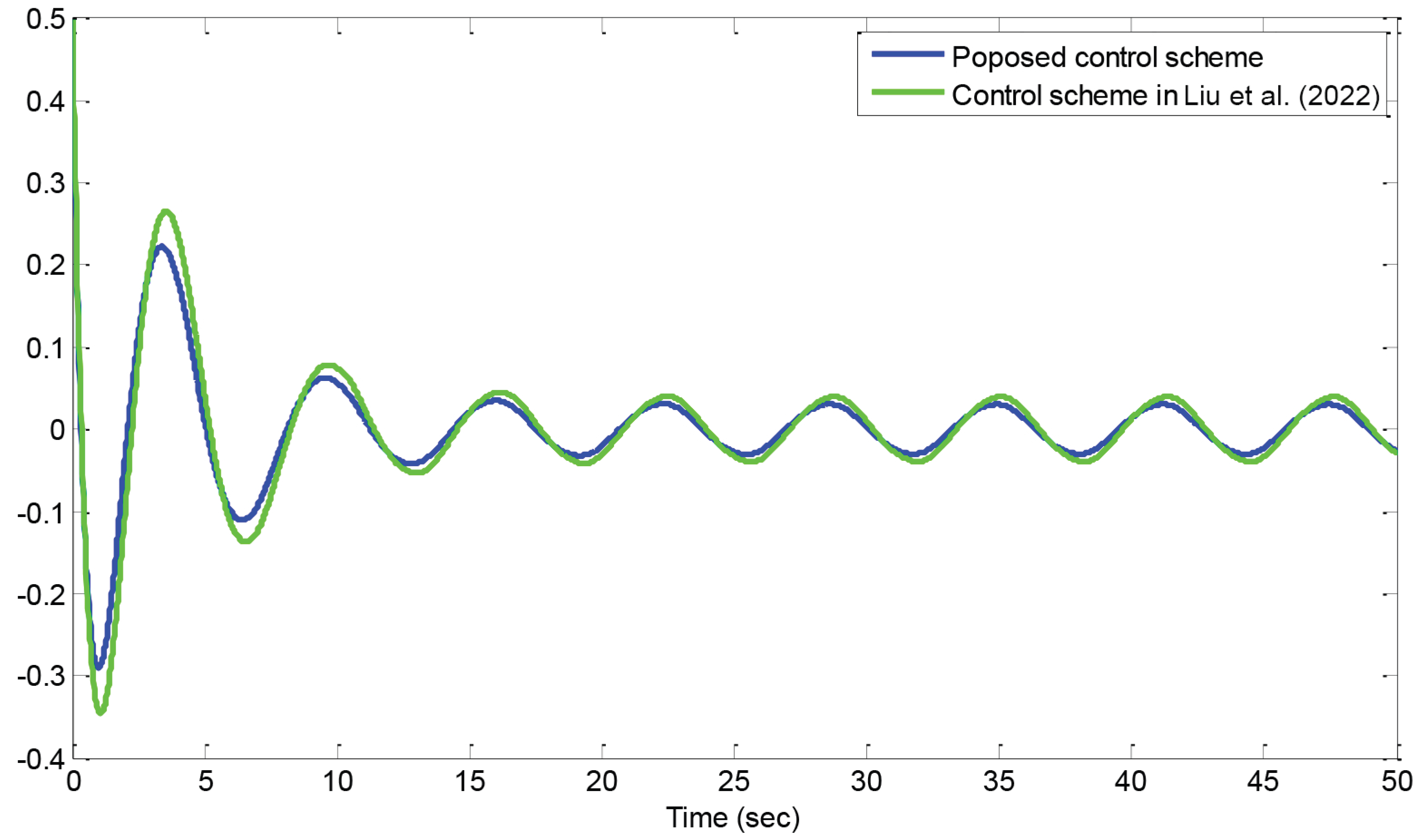
Comparative results: The proposed method is compared with an existing approach from a previous paper [40]. The existing paper addressed the problem of a nonlinear system with input delay, without considering the effect of actuator faults. Additionally, it did not utilize any funnel control scheme. In contrast, this paper introduces a funnel control method for nonlinear systems. Figure 8 presents the comparison results, demonstrating that the tracking error with the proposed method is slightly improved compared to the previous method [40], thereby confirming the effectiveness of the proposed approach.

Parameter sensitivity analysis: To further demonstrate the robustness of the proposed adaptive fuzzy funnel control scheme, a parameter sensitivity analysis is carried out by considering three different sets of controller parameters. The initial conditions are kept unchanged to ensure that the influence of the controller parameters can be evaluated independently. The initial conditions are selected as ${[{\eta }_1\left(0\right),{\eta }_2\left(0\right),{\eta }_3\left(0\right)]}^T={[0.5,0.5,0.5]}^T,$ and ${[{\widehat{\omega }}_1\left(0\right),{\widehat{\omega }}_2\left(0\right),{\widehat{\omega }}_3\left(0\right)]}^T={[0,0,0]}^T.$ The controller parameters for the three cases are chosen as follows:

• Case 1: $k_1=3$, $k_2=3$, $k_3=5$, ${\vartheta }_1={\vartheta }_2={\vartheta }_3=0.8$, $a_1=a_2=a_3=1.5$, ${\varsigma }_1={\varsigma }_2={\varsigma }_3=0.8$.
• Case 2 (Nominal Case): $k_1=4$, $k_2=4$, $k_3=6$, ${\vartheta }_1={\vartheta }_2={\vartheta }_3=1$, $a_1=a_2=a_3=2$, ${\varsigma }_1={\varsigma }_2={\varsigma }_3=1$.
• Case 3: $k_1=5$, $k_2=5$, $k_3=7$, ${\vartheta }_1={\vartheta }_2={\vartheta }_3=1.2$, $a_1=a_2=a_3=2.5$, ${\varsigma }_1={\varsigma }_2={\varsigma }_3=1.2$.

To quantitatively evaluate the influence of the controller parameters on the tracking performance, the following performance indices are adopted:

$$\begin{array}{cc}\hfill \mathrm{MAE}& =\underset{1\le t\le N}{\max }|y\left(t\right)-y_r\left(t\right)|,\hfill \end{array}$$

(73)

$$\begin{array}{cc}\hfill \mathrm{SSE}& ={\displaystyle \sum _{t=1}^N}{\left(y\left(t\right)-y_r\left(t\right)\right)}^2,\hfill \end{array}$$

(74)

$$\begin{array}{cc}\hfill \mathrm{MSE}& ={\displaystyle \frac{1}{N}}{\displaystyle \sum _{t=1}^N}{\left(y\left(t\right)-y_r\left(t\right)\right)}^2,\hfill \end{array}$$

(75)

$$\begin{array}{cc}\hfill \mathrm{RMSE}& =\sqrt{{\displaystyle \frac{1}{N}}{\sum }_{t=1}^N{\left(y\left(t\right)-y_r\left(t\right)\right)}^2},\hfill \end{array}$$

(76)

$$\begin{array}{cc}\hfill \mathrm{NMSE}& ={\displaystyle \frac{{\sum }_{t=1}^N{\left(y\left(t\right)-y_r\left(t\right)\right)}^2}{{\sum }_{t=1}^N{\left(y_r\left(t\right)-{\overline{y}}_r\right)}^2}},\hfill \end{array}$$

(77)

$$\begin{array}{cc}\hfill \mathrm{BFR}& =\left(1-{\displaystyle \frac{\sqrt{{\sum }_{t=1}^N{\left(y\left(t\right)-y_r\left(t\right)\right)}^2}}{\sqrt{{\sum }_{t=1}^N{\left(y_r\left(t\right)-{\overline{y}}_r\right)}^2}}}\right)\times 100\%.\hfill \end{array}$$

(78)

The corresponding quantitative results are summarized in

Table 1. Parameter sensitivity analysis under different controller parameter settings.

Case	MSE	RMSE	SSE	NMSE	MAE	BFR (%)
Case 1	0.0054	0.0735	0.5427	0.0115	0.0568	96.83
Case 2	0.0031	0.0557	0.3118	0.0068	0.0415	97.94
Case 3	0.0018	0.0424	0.1823	0.0041	0.0316	98.75

. It can be observed that the proposed controller maintains satisfactory tracking performance under different controller parameter settings. Although slight variations in the transient response are observed, the tracking error remains within the prescribed funnel, and all closed-loop signals remain bounded. These results demonstrate that the proposed adaptive fuzzy funnel control scheme is robust to moderate variations in the controller parameters.

Qualitative comparison with existing methods: A qualitative comparison with a number of exemplary adaptive nonlinear control systems is shown in

Table 2. Qualitative comparison of the proposed method with representative existing approaches.

Method	Actuator	Input	Funnel	Nonstrict	Stability	Complexity
	Faults	Delay	Control	Feedback
Ref. [39]	×	×	✓	×	SGUUB	Moderate
Ref. [11]	×	×	×	×	UUB	Moderate
Ref. [18]	✓	×	×	×	SGUUB	Moderate
Ref. [23]	×	✓	×	✓	SGUUB	Moderate
Proposed	✓	✓	✓	✓	SGUUB	Moderate

to further emphasize the efficacy and usefulness of the suggested adaptive fuzzy funnel control scheme. The comparison focuses on essential properties, including actuator-fault accommodation, input-delay compensation, funnel control, application to nonstrict-feedback nonlinear systems, stability guarantees, and computing complexity. It can be seen that each existing solution handles only a subset of these challenges. For example, the method in [39] constructs an adaptive finite-time fuzzy funnel controller but does not address actuator defects or input latency. Funnel control, actuator defects, and input delay are not included in the adaptive learning control approach in [11], which deals with nonlinear systems with full-state constraints. Actuator defects are compensated for by the adaptive fuzzy fault-tolerant controller suggested in [18]; however, input delay and funnel performance are not addressed. Similarly to this, the adaptive fuzzy controller in [23] takes input delay into account for nonstrict-feedback nonlinear systems but ignores funnel control and actuator defects. In contrast, the suggested approach simultaneously addresses actuator defects, input delay, and funnel performance for nonstrict-feedback nonlinear systems while assuring the semi-globally uniformly ultimately boundedness (SGUUB) of all closed-loop signals. As a result, the suggested controller offers a more thorough framework for nonlinear systems functioning under several realistic restrictions.

5. Conclusions

This study introduced an adaptive fuzzy funnel control strategy tailored for nonstrict-feedback nonlinear systems, tackling issues associated with actuator faults and input delays. The approach involved developing an adaptive funnel control mechanism using fuzzy logic systems (FLSs) to estimate unknown functions. Additionally, the Padé approximation method was employed to mitigate the impact of input delays. Integrating FLSs with the backstepping control technique guaranteed that all signals within the closed-loop system exhibited SGUUB behavior. The utilization of funnel control ensured that the tracking error remained within a predefined funnel, facilitating convergence to a specified interval through a funnel function. The practical applicability and effectiveness of the proposed controller were demonstrated through a real-world example involving an electromechanical system. Future research will focus on extending the proposed adaptive fuzzy funnel control framework to stochastic nonlinear switched systems with both actuator and sensor faults. In addition, the proposed methodology will be investigated for systems with communication constraints, event-triggered control mechanisms, and cyber–physical applications to further improve the robustness, reliability, and practical applicability of nonlinear control systems in complex and uncertain environments.