Multi-Link Kinematic Calibration with Photogrammetry

Abstract

Industrial robotic arms are fundamental components of modern automated production lines, executing critical tasks such as welding, painting, and assembly. Such high-precision operations often require careful manual tool positioning during the initial setup. To automate and refine this process, a highly accurate kinematic model of the robot is essential. In this paper, the authors propose a novel algorithm for kinematic parameter calibration using photogrammetry to track multiple robot links simultaneously. The proposed multi-link calibration approach provides a more precise parameter estimation and introduces the practical possibility of continuous parameter refinement while the robot executes its primary operational tasks. The superior accuracy and robustness of the proposed methodology are confirmed through comprehensive simulation experiments, and the feasibility of the approach is successfully demonstrated on a real robotic arm.

1. Introduction

Modern manufacturing processes frequently employ various robotic systems in automated production lines. The demand for technologically advanced and precise manufacturing continues to grow, imposing significant constraints on the positioning errors of the end-effector and its attached tools, for instance, during welding. Due to the stringent accuracy requirements, mechanical machining often relies on CNC machines rather than industrial robots [1]. Furthermore, human-like tool positioning and object manipulation tasks [2] place high demands on kinematic accuracy. Low tool positioning precision in robotic applications can stem from the manipulator’s manufacturing process, installation errors, harsh operating conditions, mechanical wear, and temperature variations [3,4].

An effective and well-known way to reduce the positioning error is calibration or refinement of the geometric parameters of the manipulator’s kinematic chain (e.g., DH parameters [5]), which involves a process of minimizing the discrepancies between the theoretical and real position of the mechanism in space [3,6]. Beyond geometric parameters, non-geometric calibration might be required to achieve high absolute accuracy. This involves compensating for factors such as joint compliance, gear backlash, and thermal expansion, which is particularly important when performing heavy-duty operations that induce elastic deformations [1,7,8]. The main component (90%) of the positioning error for a manipulator is caused by inaccurate geometric parameters of the kinematic chain [9] so this paper focuses precisely on these factors. For example, in [10], the positioning error for the ABB IRB 1600 is 2.158 mm and 0.696 mm before and after the calibration of geometric parameters, respectively. In other cases, depending on the manipulator model, positioning technique, and optimization (or identification) algorithm, the positioning accuracy after calibration improves by 3–5 times and can vary in the range of 0.08–0.5 mm [11,12]. However, kinematic accuracy and repeatability are subject to temperature and environmental conditions, as discussed in [4]. Therefore, to reach sufficient accuracy, stable environmental conditions and a proper warm-up are required. The papers [11,13,14,15] emphasize the problem of instability in the kinematic calibration of a manipulator, the importance of assessing the condition number of the Jacobian for the optimization problem, and the correct choice of the set of calibration poses or the “training set” for subsequent parameter estimation.

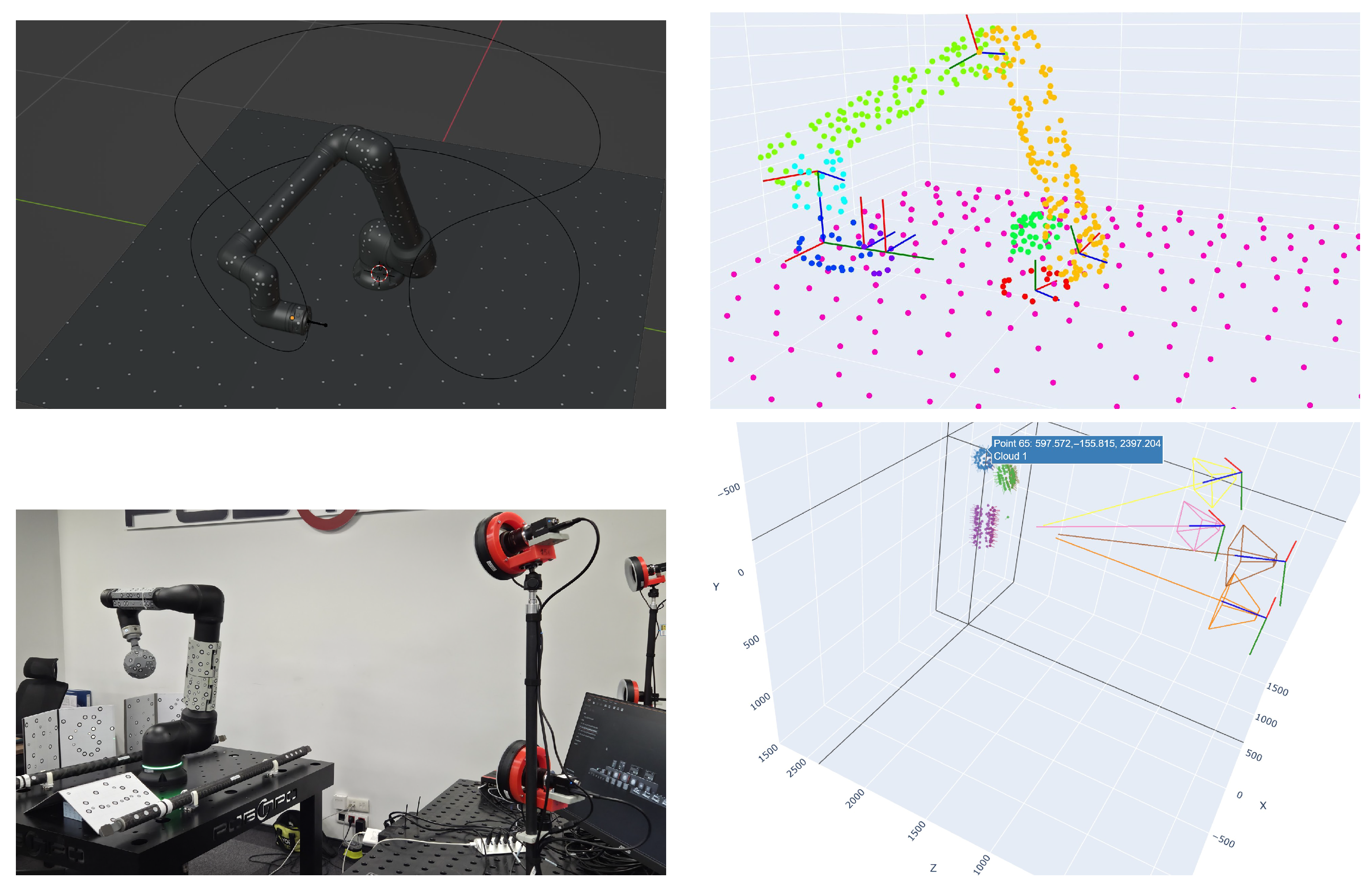
Using artificial circular markers on the surface of the robotic links (Figure 1), it is possible to track them with photogrammetry [16]. This is the key part of the authors’ kinematic calibration framework.

2. Algorithms for Calibrating Kinematic Parameters

Calibration of manipulator kinematic parameters by the end-effector is widespread and quite well represented in the scientific literature [3,11,18,19,20,21,22,23]. Calibration methods can be categorized into those with and without constraints on the manipulator’s degrees of freedom. These are commonly referred to as closed-loop and open-loop methods, respectively. In closed-loop methods, the end-effector’s movement is mechanically restricted, for example, by maintaining contact with a surface of known shape like a plane [23,24,25] or by rotating around a fixed point [26]. A mechanical loop can also be established by connecting the end-effector to a coordinate measuring machine, another manipulator, or a measuring tape [21]. Conversely, open-loop calibration methods do not impose mechanical constraints on the robot’s movement. Instead, they rely on determining the position of the end-effector using an external measuring device. For instance, a special tracking probe can be mounted on the end-effector to measure its pose with a theodolite [7] or laser tracker [10,11,23,27].

Digital camera systems [3,22], RGB-D cameras [28] and structured-light 3D scanners [12,20] are also actively employed for the calibration task. However, the performance of such vision-based approaches can be sensitive to harsh industrial conditions, such as heavy dust or smoke, occlusions, or inconsistent lighting. Consequently, calibration and primary operational tasks are typically performed at separate times. In specific applications such as robotic computed tomography, the X-ray imaging system itself can be utilized to calibrate the kinematics of the dual-robot setup [29]. With the growth of the computing power of computer systems, it becomes possible to solve more versatile and complex automation tasks like processing feedback images from computer vision systems during the work operation of the robotic system, simultaneously acquiring information about the position of various objects in the workspace. This information can be used for kinematic calibration using photogrammetry. Photogrammetry is a method for obtaining (reconstructing) 3D coordinates of points based on the analysis of digital images from one or more cameras [16,30]. This technology allows measuring highly accurate 3D coordinates of points on the surface of a robot, tool, or part in space, which makes photogrammetry a convenient tool for calibrating manipulator kinematics [3,12,22].

In this paper, similarly to [3,23], in the experimental setup, cameras observe the work area, as opposed to the scheme with a camera or sensors mounted on the robot [12,29]. Observation of the workspace by multiple cameras allows simultaneous tracking of multiple robotic links (or corresponding point clouds), which is the basis of the new approach proposed by the authors for multi-link kinematic calibration. To the best of the authors’ knowledge, utilizing simultaneous multi-link photogrammetric tracking for kinematic calibration represents a highly novel approach that has not been previously encountered in the literature, as prior works predominantly focus solely on end-effector tracking.

The proposed multi-link approach offers several significant advantages over traditional single-link methods. First, it enables the utilization of a substantially broader range of robot configurations, particularly in practical scenarios where the end-effector might be partially or entirely occluded from camera views. Second, by incorporating spatial data from multiple links simultaneously, the overall robustness and accuracy of the kinematic calibration are notably enhanced. Finally, continuous multi-link spatial tracking introduces the possibility of performing dynamic calibration concurrently with the robot’s primary operational tasks. In the proposed methodology, close-range photogrammetry utilizing artificial retro-reflective circular markers (or targets) serves as a fundamental building block. In contrast to other modern approaches relying on RGB-D cameras [28] or X-ray sensors [29], close-range photogrammetry can compete directly with laser trackers in terms of accuracy [16,30]. The effectiveness of the proposed method is verified in the experimental part.

While the transition to a multi-link formulation inherently increases the dimensionality of the objective function, modern computational frameworks effectively manage this complexity. To efficiently solve the expanded optimization problem and refine the kinematic model parameters via the Levenberg–Marquardt method, the analytical Jacobian is computed using automatic differentiation tools from a Python 3.12 machine learning library JAX [31], similarly to [29]. An open-source Python library [32] demonstrates a real-time solution for the inverse kinematics problem for heavy closed-loop chains using JAX-based Jacobian estimation for Levenberg–Marquardt optimization.

3. Mathematical Problem Statement

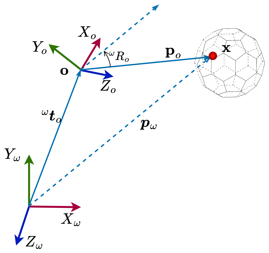
Bold font will be used to denote vector quantities, and uppercase for matrices. The position of a rigid body (robot links, tools, etc.) relative to a certain coordinate frame (CF) is described by a transformation matrix ${}^{w}M_o\in \mathit{SE}\mathbf{3}$, which maps the 3D coordinates of a point of this body into the new CF (Figure 2):

$${\mathit{p}}_w={}^{w}M_o·{\mathit{p}}_o=\left[\begin{array}{cc}{}^{w}R_o^{3\times 3}& {}^w\mathit{t}_o\\ {\mathbf{0}}^T& 1\end{array}\right]\left[\begin{array}{c}{x}_o\\ y_o\\ z_o\\ 1\end{array}\right]$$

(1)

• ${}^w\mathit{t}_o$—defines three degrees of freedom, the position of the center of the local CF of the object relative to the World CF (WF) (it is convenient to tie the WF to the measuring system—the master camera in photogrammetry or a laser tracker);
• ${\mathit{p}}_o\in {\mathbb{R}}^3$—local homogeneous (the last dimension is auxiliary and needed only for the brevity of algebraic notations) 3D coordinates of a point relative to the object CF;
• ${\mathit{p}}_w\in {\mathbb{R}}^3$—position of the point in the WF;
• ${}^{w}R_o^{3\times 3}\in \mathit{SO}\mathbf{3}$—rotation matrix (constructed from three rotation angles using Rodrigues’ formula or the Euler angles formula [33,34,35]);
• $\mathit{SO}\mathbf{3}\subset {\mathbb{R}}^{3\times 3}$—special orthogonal group of rotations: ${}^{w}R_o^T={}^{w}R_o^{-1}$, $det{(}^w{R}_o)=1$;
• $\mathit{SE}\mathbf{3}\subset {\mathbb{R}}^{4\times 4}$—Euclidean motion group [33,36] or similarity transformation with unit scale, describes the movement of a rigid body in space.

Thus, the kinematic model of an n-link robot is described by a chain of transformations:

$${}^{b}M_{l_n}={}^{b}M_{{\mathit{l}}_1}·{}^{l_1}M_{{\mathit{l}}_2}\dots {}^{l_{i-1}}M_{{\mathit{l}}_i}\dots {}^{l_{n-1}}M_{{\mathit{l}}_n},$$

(2)

${}^{b}M_{l_n}\in \mathit{SE}\mathbf{3}$—position of the end-effector link $l_n$ relative to the robot base CF b or $l_0$. For a manipulator having r and p revolute and prismatic joints, respectively, the minimum number of parameters for the robot model will be $4r+2p+6$ [19]. This sum also includes the transformation between the WF and the robot base, as well as the end-effector link and the tool, since in practice (2) has the following form:

$${}^{w}M_t={}^{w}M_b{}^{b}M_{l_n}{}^{l_n}M_t,$$

(3)

${}^{w}M_t\in \mathit{SE}\mathbf{3}$—tool position relative to the measuring system; ${}^{l_n}M_t\in \mathit{SE}\mathbf{3}$—tool position relative to the end-effector link.

The kinematic model of the manipulator (3) relies on parameters that define the spatial transformations ${}^{l_{i-1}}M_{l_i}$ between adjacent links. The Denavit–Hartenberg (DH) parameterization scheme is the most widely known convention [5]:

$${}^{l_{i-1}}M_{l_i}({\theta }_i,d_i,a_i,{\alpha }_i)=R_z\left({\theta }_i\right)T_z\left(d_i\right)T_x\left(a_i\right)R_x\left({\alpha }_i\right),$$

(4)

• $T_{·}(·)\in \mathit{SE}\mathbf{3}$—linear translation matrix along the corresponding CF axis. The translations $d_i$ (link offset along the Z axis) and $a_i$ (link length along the X axis) are constant for any configuration of a robot with revolute joints;
• $R_x\left({\alpha }_i\right)\in \mathit{SE}\mathbf{3}$—rotation matrix around the X axis of the link $l_i$ CF by an angle ${\alpha }_i$ (link twist), constant for any robot configuration;
• $R_z\left({\theta }_i\right)\in \mathit{SE}\mathbf{3}$—rotation matrix around the Z axis of the link $l_{i-1}$ CF by an angle ${\theta }_i$ (joint angle), variable for a robot with revolute joints. It includes the actuator rotation angle $q_i$ and a constant correction (zero offset): ${\theta }_i=q_i+{\mathsf{\Delta }}_{{\theta }_i}$. For simplicity, without loss of generality, we will further consider a robot manipulator with revolute joints.

Using photogrammetry (next section), one can obtain the tool position ${}^{w}M_{t,j}$ at a specific moment in time $j\in [1..m]$ for the corresponding robot configuration ${\left\{{\mathit{q}}_j\right\}}_{j=1}^m,{\mathit{q}}_j={(q_{1,j},\dots ,q_{n,j})}^T$. Thus, the task of kinematic calibration consists of solving Equation (3) in the form:

$${}^{w}M_{t,j}^{-1}{}^{w}M_b{}^{b}M_{l_n}\left({\mathit{q}}_j\right){}^{l_n}M_t=I_{4\times 4},$$

(5)

for m different configurations with a known ${}^{w}M_{t,j}$. Let us separate the known part and the unknown part from the DH parameters:

$$\begin{array}{c}\hfill {\mathsf{\theta }}_j={\mathit{q}}_j+{\mathsf{\Delta }}_{\mathsf{\theta }},\\ \hfill \mathit{d}={\mathit{d}}_0+{\mathsf{\Delta }}_{\mathit{d}},\\ \hfill \mathit{a}={\mathit{a}}_0+{\mathsf{\Delta }}_{\mathit{a}},\\ \hfill \mathsf{\alpha }={\mathsf{\alpha }}_0+{\mathsf{\Delta }}_{\mathsf{\alpha }},\end{array}$$

(6)

• ${\mathit{q}}_j\in {\mathbb{R}}^n$—known vector of actuators rotation angles for the j-th manipulator configuration;
• ${\mathit{d}}_0,{\mathit{a}}_0,{\mathsf{\alpha }}_0\in {\mathbb{R}}^n$—parameters usually known from the specification;
• ${\mathsf{\Delta }}_{·}\in {\mathbb{R}}^n$—the unknown corrections to be estimated for the model parameters. Let us combine the target parameters into the vector ${\mathsf{\Delta }}_{\mathit{x}}={({{\mathsf{\Delta }}_{\mathsf{\theta }}}^T,{{\mathsf{\Delta }}_{\mathit{d}}}^T,{{\mathsf{\Delta }}_{\mathit{a}}}^T,{{\mathsf{\Delta }}_{\mathsf{\alpha }}}^T)}^T\in {\mathbb{R}}^{4n}$.

Considering that the position of the robot base ${}^{w}M_b$ in the WF and the tool position ${}^{l_n}M_t$ on the robot (comprising 12 degrees of freedom in total) also require estimation, Equation (3) initially yields $4n+12$ independent unknowns. However, studies [11,12,37] note that the parameters defining the base frame ${}^{w}M_b$ are mathematically coupled (inseparable) with the first joint’s parameters ${\mathsf{\Delta }}_{{\theta }_1},{\mathsf{\Delta }}_{d_1}$. Similarly, the tool frame parameters ${}^{l_n}M_t$ are inseparable from the parameters of the end-effector link ${\mathsf{\Delta }}_{{\theta }_n},{\mathsf{\Delta }}_{d_n},{\mathsf{\Delta }}_{a_n},{\mathsf{\Delta }}_{{\alpha }_n}$. To avoid kinematic parameter redundancy and singularities during optimization, these six DH parameters can be treated as constants, leaving only a subset to be optimized. For brevity, let us denote this reduced subset as ${\mathsf{\Delta }}_{\mathit{x}}\in {\mathbb{R}}^{4n-6}$. Thus, the final number of effectively independent unknowns in (3) becomes $4n+12-6=4n+6$ [19]. For instance, the kinematic model (3) for the robot shown in Figure 1 includes $4·6+6=30$ parameters optimized during calibration, 18 of which are internal DH parameters ${\mathsf{\Delta }}_{\mathit{x}}$.

The set of m observed configurations allows formulating the optimization problem for the kinematic calibration:

$$\begin{array}{c}\hfill {\mathsf{\Delta }}_{\mathit{x}}^{\ast },{}^{w}M_b^{\ast },{}^{l_n}M_t^{\ast },=\underset{\begin{array}{c}{\mathsf{\Delta }}_{\mathit{x}}\in {\mathbb{R}}^{4n-6},\\ {}^{w}M_b\in \mathit{SE}\mathbf{3},\\ {}^{l_n}M_t\in \mathit{SE}\mathbf{3}\end{array}}{\mathrm{argmin}}\mathcal{L}({\mathsf{\Delta }}_{\mathit{x}},{}^{w}M_b,{}^{l_n}M_t),\\ \hfill \mathcal{L}({\mathsf{\Delta }}_{\mathit{x}},{}^{w}M_b,{}^{l_n}M_t)={\displaystyle \sum _{j=1}^m}{\displaystyle \sum _{k=1}^8}\left|\right|{\mathit{e}}_{j,k}{\left|\right|}_2^2.\end{array}$$

(7)

The spatial residual vector ${\mathit{e}}_{j,k}\in {\mathbb{R}}^3$ represents the 3D deviation for point k in configuration j:

$${\mathit{e}}_{j,k}{=}^{ w}{M}_{t,j}^{-1}·{}^{w}M_b·{}^{b}M_{l_n}({\mathit{q}}_j,{\mathsf{\Delta }}_{\mathit{x}})·{}^{l_n}M_t·{\mathit{p}}_k-{\mathit{p}}_k,$$

(8)

where ${\mathit{p}}_k$ denotes the eight predefined bounding box corner points of the end-effector or tool.

The strategic incorporation of these bounding boxes points to the cost function, which provides several critical advantages. First, it naturally unifies orientation and translation errors into a single, physically meaningful metric (Euclidean distance). Directly penalizing rotation matrices and translation vectors usually requires assigning arbitrary weighting factors to balance radians and millimeters. By evaluating the spatial residuals of the bounding box corners, angular and positional discrepancies are inherently balanced according to the actual physical dimensions of the tracked link. Second, it significantly improves the numerical stability of the gradient estimation. Directly minimizing angular deviations often involves the inverse cosine function (arccos, inverse Rodrigues’ formula [33]), whose derivative approaches infinity as the target angle error nears zero. Point-based $L_2$-norm residuals bypass this particular singularity completely, ensuring robust gradient convergence during optimization. Finally, utilizing just the eight corner points is mathematically sufficient to fully constrain the spatial 3D pose.

Assuming the parameterization scheme ${}^{l_{i-1}}M_{l_i}$ is appropriately chosen and initialized with accurate a priori estimates, the optimization problem (7) can be efficiently solved using numerical techniques such as the Gauss–Newton or Levenberg–Marquardt algorithms [11,19]. However, the classical DH convention (4) exhibits singularities for pairs of joints with parallel or near-parallel axes. This is caused by the linear dependency between the parameters $d_{i-1}$ and $d_i$, which severely degrades the numerical stability of the optimization (7). To address this, several studies employ a combined DH parameterization [11,12]:

$${}^{l_{i-1}}M_{l_i}({\theta }_i,d_i,a_i,{\alpha }_i,{\beta }_i)=R_z\left({\theta }_i\right)T_z\left(d_i\right)T_x\left(a_i\right)R_x\left({\alpha }_i\right)R_y\left({\beta }_i\right).$$

(9)

Depending on whether the adjacent joint axes are orthogonal or parallel, either ${\beta }_i$ or $d_i$ is kept fixed, respectively.

Consequently, the kinematic model (3) remains non-redundant (strictly four parameters per link) and computationally stable during the calibration process. Once the optimal parameters are identified, the calibrated combined DH model can be seamlessly converted back to the standard DH representation (or any other convention) using the algorithm proposed in [35]. The following section details how the unknown spatial poses ${}^{w}M_{t,j}$ can be acquired via photogrammetry to facilitate this kinematic calibration.

4. Multi-Link Calibration with Photogrammetry

Photogrammetry, as a 3D reconstruction technology, is widely used, for example, in aerial photography to build a 3D model of the landscape by analyzing natural texture features on the earth’s surface (buildings, roads, trees, etc.). In fact, the main requirement for photogrammetry during measurements is the presence of contrasting texture features on the object’s surface in order to obtain an accurate 3D model. In this paper, for the best accuracy and reliability of the result, the authors used artificial circular markers widely used in industrial photogrammetry [16,30,34,38,39]. We also note that photogrammetry is often primarily used to obtain the 3D coordinates of surface points, but in this context, the primary task is determining the position of the robot links in space (pose tracking).

A custom implementation of photogrammetry algorithms was utilized to conduct the robot kinematic calibration experiments, analyzing images of circular markers attached to the surfaces of each moving link and the ground plane. While the comprehensive details of this photogrammetric pipeline are elaborated in [16], its key aspects relevant to this study are summarized below. The algorithms initially identify high-contrast texture features (circular markers) located on the surfaces of different robot links. Subsequently, numerical optimization is employed to compute the 3D coordinates of these markers, segmenting them into distinct point clouds for each link (illustrated by differently colored dots in Figure 1). Crucially, the photogrammetry system estimates the spatial poses of these 3D point clouds over time relative to the main camera’s CF.

To achieve high precision in both 3D coordinate reconstruction and link pose tracking, photogrammetry typically requires a large dataset of images captured from multiple viewpoints, in addition to the use of high-contrast markers [16]. Mathematically, moving the camera (or cameras) around a stationary object is fundamentally equivalent to moving the object in front of a stationary camera rig. Consequently, an automated robotic capture process proves highly advantageous. This approach enables the simultaneous acquisition of the data needed for both kinematic parameter identification (e.g., ${\mathsf{\Delta }}_{\mathit{x}}$) and photogrammetric tracking (3D coordinates and time-varying spatial poses ${}^{w}M_{c_i,j}\in \mathit{SE}\mathbf{3}$) within a single, unified procedure. In the physical experimental setup, a multi-camera rig comprising four 12-megapixel HikRobot industrial global-shutter cameras was employed (refer to the bottom row of Figure 1). The primary stages of this photogrammetric pipeline are as follows:

(1)

acquiring 2D images of the robot’s motion using the multi-camera rig, synchronously logging the joint configurations ${\left\{{\mathit{q}}_j\right\}}_{j=1}^m$ at every discrete time step $j\in [1..m]$;

(2)

matching observed 2D features across multiple camera views to reconstruct 3D point clouds for each moving link ${\{{\mathit{p}}_{i,k}\in {\mathbb{R}}^3\}}_{k=1}^{N_{pts}^i},i\in [1..n]$ within an independent local CF $c_i$ (the origin is located at the center of mass, and the coordinate axes are aligned with the principal directions of the point cloud);

(3)

Aggregating 2D markers by their corresponding 3D links and calculating the spatial pose of each link’s point cloud ${}^{w}M_{c_i,j}\in \mathit{SE}\mathbf{3}$ relative to the World Frame (WF), which is anchored to the main camera.

With the spatial poses of the links ${}^{w}M_{c_i,j}$ obtained, the objective function from (7) must be reformulated to accommodate multi-link kinematic calibration:

$$\mathcal{L}({\mathsf{\Delta }}_{\mathit{x}},{}^{w}M_b,{}^{l_1}M_{c_1},\dots ,{}^{l_n}M_{c_n})={\displaystyle \sum _{i=1}^n}{\displaystyle \sum _{j=1}^m}{\displaystyle \sum _{k=1}^8}\left|\right|{\mathit{e}}_{i,j,k}{\left|\right|}_2^2,$$

(10)

where the multi-link spatial residual vector ${\mathit{e}}_{i,j,k}\in {\mathbb{R}}^3$ is defined for each tracked link i:

$${\mathit{e}}_{i,j,k}{=}^{ w}{M}_{c_i,j}^{-1}·{}^{w}M_b·{}^{b}M_{l_i}({\mathit{q}}_j,{\mathsf{\Delta }}_{\mathit{x}})·{}^{l_i}M_{c_i}·{\mathit{p}}_{i,k}-{\mathit{p}}_{i,k}.$$

(11)

Simultaneously, a fixed transformation representing the relative pose between each point cloud CF and its corresponding link CF is introduced into the set of parameters to be estimated: ${}^{l_i}M_{c_i}\in \mathit{SE}\mathbf{3}$. Similarly to the previous definition, ${\mathit{p}}_{i,k}$ denotes the link i bounding box corner points. Conceptually, this scheme extends the standard approach: instead of relying exclusively on the tool CF (t in ${}^{l_n}M_t$) as seen in problem (7), the multi-link formulation (10) independently utilizes the CF of the surface point cloud attached to each individual link ($c_i$ in ${}^{l_i}M_{c_i}$). As in (7), the optimization aims to minimize the spatial residuals between the measured link poses and the poses predicted by the kinematic model.

It is worth noting that while the multi-link formulation (10) increases the total number of unknowns compared with the single-link version (7), there is a huge benefit due to the increase in quadratic terms within the objective function because the total number of residual equations scales linearly with the number of calibration configurations m. A clear comparison of the equation-to-unknown ratios for both approaches is provided in

Table 1. Settings for kinematic calibration.

Problem	Quantity
	Calibration Configurations	$\mathit{x},\mathit{y},\mathit{z}$-Residual Equations	Unknowns
Single-link calibration	200	4800	30
	100	2400
	50	1200
	25	600
	13	312
Multi-link calibration	200	28,800	60
	100	14,400
	50	7200
	25	3600
	13	1872

.

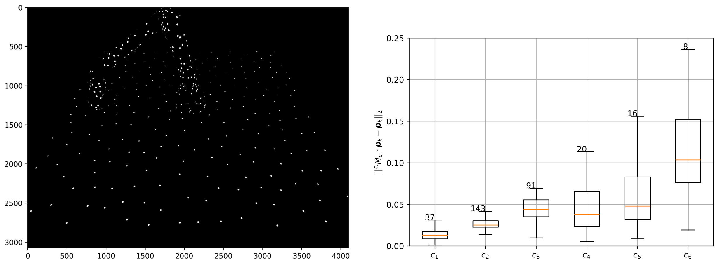
To evaluate the capability of the selected photogrammetric pipeline to solve the multi-link tracking problem, simulated source images were generated by rendering an animated robot model within the Blender3D environment (simulating observation via a multi-camera rig continuously tracking attached high-contrast markers), left image in Figure 3. By utilizing the known ground-truth positions (${}^{c_i}M_{c_i}={}^{w}M_{c_i}^{-1 }{}^{w}M_{c_i}^{\mathit{GT}}$), the accuracy of the photogrammetric tracking as point position error can be carefully assessed, as illustrated in Figure 3. The figure visualizes the distribution of point position errors ($L_2$-norm) using box-and-whisker plots. Each distribution aggregates position errors using the link’s cloud points coordinates $p_k$ across $m=10$ distinct spatial configurations of the robot.

As depicted in Figure 3, the photogrammetric tracking error for links 1 through 5 remains tightly constrained, not exceeding 0.16 mm (in terms of whisker span, which encompasses approximately 99% of the measurements). For the end-effector link, the error reaches 0.25 mm. A primary factor influencing pose estimation accuracy is the quantity of visible markers on a given link at any temporal instance, indicated above each box plot. Empirical observations suggest that maintaining a minimum of 20 visible markers per link yields optimal tracking performance.

For the real-world experiment (bottom left image in Figure 1), photogrammetric carbon-fiber scale bars were placed into the test scene to resolve scale ambiguity [16]. The scale bars were calibrated in advance, with the distances between their targets measured using precise metrological equipment. The accuracy of the point-wise measurements was validated against these scale bars, ensuring that the spatial error of the reconstructed point clouds remains below 0.1 mm. Markers were attached to the robot using custom 3D-printed sleeves and an end-effector fixture. All three parts (the two sleeves and the end-effector fixture) act as rigid bodies with an associated 3D point cloud of markers in their respective local coordinate frames, which are used for tracking their poses relative to the main camera (bottom right image in Figure 1). To compute the intrinsic 3D layout of the point clouds associated with the mechanical links, the same set of robot configurations acquired for kinematic calibration is utilized. However, unlike the approach in [12], the estimation of the rigid point clouds is mathematically decoupled from the actual kinematic parameter calibration. This allows the point clouds for the sleeves to be estimated once and seamlessly reused to calibrate multiple physical robots of the same model. If some markers on a sleeve become damaged during usage, or if a completely different robot model requires tracking, the point cloud reconstruction only has to be repeated for the affected or new sleeve. This modularity makes the process highly flexible. A notable limitation of the vision-based photogrammetry system is its inability to operate reliably in environments with heavy dust and smoke, such as during automated welding. Nonetheless, the inherent redundancy of simultaneously tracking multiple links across a multi-camera rig provides a higher resilience to partial occlusions and environmental degradation than conventional single-target laser-tracker configurations.

5. Multi-Link Calibration Stability

To illustrate the inner structure of the calibration problems, let ${\mathit{e}}_i\in {\mathbb{R}}^{24m}$ denote the stacked vector of spatial residuals over all m configurations and 8 bounding box points for link i, and ${{\mathsf{\Delta }}_{\mathit{x}}}^{\left(k\right)}$ represent the subset of active DH parameters associated with link k. It should be noted that some internal parameter sub-vectors ${{\mathsf{\Delta }}_{\mathit{x}}}^{\left(k\right)}$ can have zero length if their respective parameters are not optimized to prevent the previously discussed theoretical redundancy, and the partial derivatives for the external frame alignments (${}^{w}M_b$ and ${}^{l_i}M_{c_i}$) are omitted in this schematic for brevity. For a 6-DoF robot ($n=6$, yielding 18 optimized DH parameters), the conventional single-link Jacobian $J_{EE}\in {\mathbb{R}}^{24m\times 18}$ for the optimization problem (7) (tracking only Link 6) takes the following dense form:

$$J_{EE}=\left[\begin{array}{cccccc}{\displaystyle \frac{\partial {\mathit{e}}_6}{\partial {\mathsf{\Delta }}_{\mathit{x}}^{\left(1\right)}}}& {\displaystyle \frac{\partial {\mathit{e}}_6}{\partial {\mathsf{\Delta }}_{\mathit{x}}^{\left(2\right)}}}& {\displaystyle \frac{\partial {\mathit{e}}_6}{\partial {\mathsf{\Delta }}_{\mathit{x}}^{\left(3\right)}}}& {\displaystyle \frac{\partial {\mathit{e}}_6}{\partial {\mathsf{\Delta }}_{\mathit{x}}^{\left(4\right)}}}& {\displaystyle \frac{\partial {\mathit{e}}_6}{\partial {\mathsf{\Delta }}_{\mathit{x}}^{\left(5\right)}}}& {\displaystyle \frac{\partial {\mathit{e}}_6}{\partial {\mathsf{\Delta }}_{\mathit{x}}^{\left(6\right)}}}\end{array}\right].$$

(12)

In contrast, when simultaneously tracking Link 2, Link 3, and Link 6 for the multi-link optimization problem (10), the spatial pose of a proximal link (one closer to the robot base) depends solely on its preceding parameters, resulting in strictly zero partial derivatives with respect to any subsequent distal links (those further from the robot base). Consequently, the concatenated multi-link Jacobian $J_{multi}\in {\mathbb{R}}^{72m\times 18}$ expands into a block lower-triangular structure:

$$J_{multi}=\left[\begin{array}{cccccc}{\displaystyle \frac{\partial {\mathit{e}}_2}{\partial {\mathsf{\Delta }}_{\mathit{x}}^{\left(1\right)}}}& {\displaystyle \frac{\partial {\mathit{e}}_2}{\partial {\mathsf{\Delta }}_{\mathit{x}}^{\left(2\right)}}}& \mathbf{0}& \mathbf{0}& \mathbf{0}& \mathbf{0}\\ {\displaystyle \frac{\partial {\mathit{e}}_3}{\partial {\mathsf{\Delta }}_{\mathit{x}}^{\left(1\right)}}}& {\displaystyle \frac{\partial {\mathit{e}}_3}{\partial {\mathsf{\Delta }}_{\mathit{x}}^{\left(2\right)}}}& {\displaystyle \frac{\partial {\mathit{e}}_3}{\partial {\mathsf{\Delta }}_{\mathit{x}}^{\left(3\right)}}}& \mathbf{0}& \mathbf{0}& \mathbf{0}\\ {\displaystyle \frac{\partial {\mathit{e}}_6}{\partial {\mathsf{\Delta }}_{\mathit{x}}^{\left(1\right)}}}& {\displaystyle \frac{\partial {\mathit{e}}_6}{\partial {\mathsf{\Delta }}_{\mathit{x}}^{\left(2\right)}}}& {\displaystyle \frac{\partial {\mathit{e}}_6}{\partial {\mathsf{\Delta }}_{\mathit{x}}^{\left(3\right)}}}& {\displaystyle \frac{\partial {\mathit{e}}_6}{\partial {\mathsf{\Delta }}_{\mathit{x}}^{\left(4\right)}}}& {\displaystyle \frac{\partial {\mathit{e}}_6}{\partial {\mathsf{\Delta }}_{\mathit{x}}^{\left(5\right)}}}& {\displaystyle \frac{\partial {\mathit{e}}_6}{\partial {\mathsf{\Delta }}_{\mathit{x}}^{\left(6\right)}}}\end{array}\right].$$

(13)

To provide strong evidence of this structural advantage, consider a scenario where both approaches rely on the exact same amount of observational data. Let the conventional single-link calibration (7) acquire m end-effector configurations, providing $24m$ residual equations. Alternatively, let the proposed multi-link strategy (10) use $m^{\prime }$ configurations tracking three links, providing $72m^{\prime }$ residuals. Even if the amount of available residuals is equalized ($24m=72m^{\prime }$, meaning $m=3m^{\prime }$), the resulting Jacobian structures are remarkably different.

While increasing configurations reduces statistical noise, the single-link Jacobian $J_{EE}$ simply becomes a taller dense matrix. It fails to efficiently eliminate the mathematical coupling among the internal Denavit–Hartenberg parameters. Because $J_{EE}$ lacks constraints on intermediate geometry, the optimization is prone to overfitting. The proximal parameters typically become the “victims” of this process; being furthest from the only observed point (the end-effector), they can be artificially distorted by the solver to incorrectly compensate for smaller parameter errors in the distal links.

In contrast, the multi-link Jacobian $J_{multi}$ features a vast number of exact zeros forming a block lower-triangular structure. These zero blocks structurally decouple the estimated parameters. Because distal parameters have no mathematical influence on the proximal spatial residuals, the proximal parameters are strictly anchored by their own local observations at the intermediate links.

Another practical approach to evaluate how well the parameters can be estimated via a Gauss–Newton-like process (e.g., the Levenberg–Marquardt algorithm) is by examining the condition number c of the approximate Hessian $H=J^{T}J$:

$$c={\displaystyle \frac{{\lambda }_{max}}{{\lambda }_{min}}}$$

(14)

where ${\lambda }_{max}$ and ${\lambda }_{min}$ are the maximum and minimum eigenvalues of H, respectively. Fundamentally, the condition number acts as an error amplification factor that dictates how observational noise within the spatial residuals propagates into the variance of the estimated parameters. A lower condition number implies better linear independence of the Jacobian columns, greater numerical stability, and inherently higher resilience to measurement noise. Results supporting these conclusions for the multi-link calibration are presented in the experimental section.

6. Initial Estimation for the Multi-Link Calibration

The objective functions for both single-link (7) and multi-link (10) calibration represent highly non-linear optimization problems. As with most numerical optimization techniques (e.g., Levenberg–Marquardt), convergence to the global minimum is heavily dependent on the quality of the initial parameter estimates. Therefore, before refining the kinematics, it is crucial to perform a robust, mathematically structured initial estimation of the spatial alignments, specifically the location of the robot base ${}^{w}M_b$ and the cloud-to-link transformations ${}^{l_i}M_{c_i}$. This estimation process is well known as the classical hand-eye calibration problem, fundamentally formulated as solving matrix equations of the form $AX=XB$ or $AX=YB$ on the Euclidean group [33,40,41].

Based on (3), to establish the initial approximation for each cloud-to-link (or “${\mathrm{hand}\text{-}\mathrm{eye}}^{-1}$” (where both “eye” and “cloud”, as well as “link” and “hand”, denote the same CFs) rigid transformation ${}^{l_i}M_{c_i}$ and the overall global transformation base-to-camera ${}^{w}M_b$, the measured spatial relationships at any timestamp j can be reorganized as slightly modified $AX=YB$:

$$A_j=Y·B_j·X_i,$$

(15)

where:

• $A_j={}^{w}M_{c_i,j}$ represents the spatial pose of the link’s point cloud directly measured by the photogrammetry tracking system;
• $B_j={}^{b}M_{l_i}\left({\mathit{q}}_j\right)$ is the pose calculated using the nominal a priori forward kinematics based on the current actuator angle;
• $Y={}^{w}M_b$ is the shared, globally unknown base-to-camera transformation (constant across the entire setup);
• $X_i={}^{l_i}M_{c_i}$ is the unknown cloud-to-link transformation mapping the photogrammetric markers (also known as targets) to the respective link frame (constant for a specific link i).

Structuring the problem as $A_j=Y·B_j·X_i$ allows for the decoupling of the unknown variables. By analyzing the relative motion between two discrete temporal frames, $j_1$ and $j_2$, the static internal transformation $X_i$ cancels out mathematically:

$$A_{j_2}·A_{j_1}^{-1}=Y·B_{j_2}·B_{j_1}^{-1}·Y^{-1}.$$

(16)

With sufficient non-degenerate relative motions, the global frame alignment Y (${}^{w}M_b$) can be robustly identified using standard closed-form algebraic solutions [33,40]. Following the determination of Y, the link-specific initial approximations $X_i$ (${}^{l_i}M_{c_i}$) are recovered in a similar manner. The resulting initial estimates reduce the risk of falling into local minima during the subsequent Levenberg–Marquardt non-linear optimization of the complete multi-link formulation (10).

7. Computational Experiment Results

The experimental part consists of a computational experiment with known ground truth data and the real experiment based on data captured from two different robots of the same model (used and brand new), as shown in Figure 1. In both cases, kinematic calibration was performed using two approaches: the conventional single-link formulation (7), which tracks only the end-effector link, and the proposed multi-link formulation (10), which simultaneously tracks the poses of multiple links. In all cases, tracking was conducted using photogrammetry.

The computational experiment utilized synthetic data generated in the Blender3D modeling environment [17]. To evaluate the robustness of the calibration against possible real-world positioning errors, random noise was injected into the tracked poses of the links. This noise level intentionally exceeded typical photogrammetry tracking deviations to more clearly illustrate the performance differences between the comparative methods. The added tracking errors were uniformly distributed, with linear and angular deviations bounded by $\pm 10$ mm and $\pm 5$ degrees, respectively. The parameter settings for both optimization tasks are detailed in Table 1. The number of residual equations corresponds to the scalar x, y, and z coordinate constraints evaluated within the objective function of the calibration problems (7) and (10).

The accuracy of the resulting kinematic models was evaluated on an independent test set of $m_t=100$ robot configurations, distinct from the calibration dataset. This evaluation relies on an objective function where the calibrated DH parameters ${\mathsf{\Delta }}_{\mathit{x}}$ are held constant:

$$\mathcal{L}({}^{w}M_b,{}^{l_n}M_{c_n})={\displaystyle \sum _{j=1}^{m_t}}{\displaystyle \sum _{k=1}^8}\left|\right|{\mathit{e}}_{n,j,k}{\left|\right|}_2^2.$$

(17)

As previously defined in (11), the spatial residual vector ${\mathit{e}}_{n,j,k}$ represents the deviation of the bounding box points attached to the end-effector link (link n) at each configuration step $j\in [1..m_t]$. These deviations quantify the discrepancy between the point poses determined by the spatial tracking system and those predicted by the robot’s forward kinematic model. In essence, evaluating this metric requires solving a reduced version of (7) that estimates only the minimal necessary subset of parameters: the transformation of the robot base relative to the WF ${}^{w}M_b$, and the relative transformation between the end-effector link and its corresponding CF ${}^{l_n}M_{c_n}$. Optimizing this localized subset minimizes the influence of reference frame misalignment, allowing for a pure assessment of the predicted tool pose based solely on the quality of the calibrated DH parameters. This methodology enables an objective comparison between parameter sets obtained via fundamentally different calibration schemes. Furthermore, this assessment technique remains broadly compatible with various end-effector tracking devices, including photogrammetry setups, laser trackers, and coordinate measuring machines.

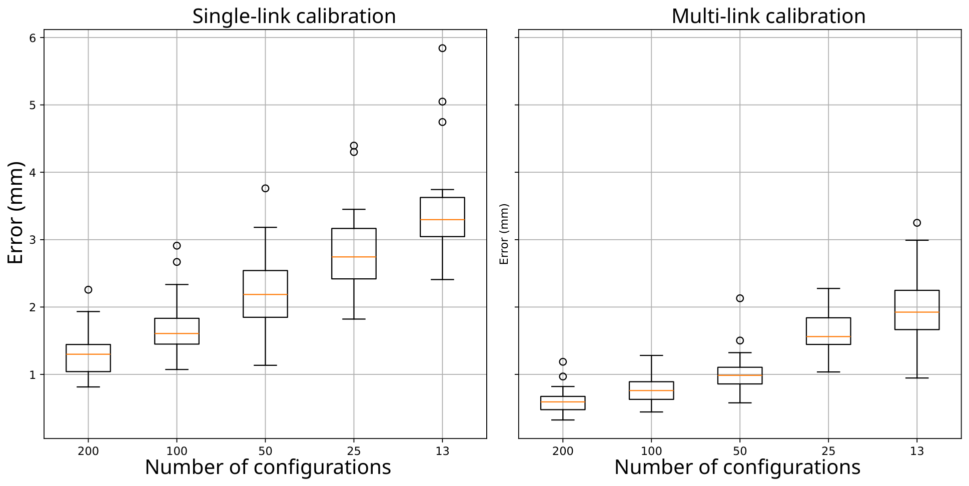
Subsequently, across Figure 4, the resulting end-effector positioning error (17) (vertical axis) achieved by the DH parameters calibrated under both multi-link and single-link approaches is illustrated. This tracking error is evaluated against different numbers of robot calibration configurations used for optimization (horizontal axis). As previously stated, these tracked poses were intentionally corrupted with uniform noise up to 10 mm in translation and 5° in rotation to rigorously stress-test the algorithms. The plot clearly demonstrates the superior robustness and accuracy of the proposed multi-link technique. Even in the presence of severe tracking noise during calibration, the multi-link kinematic calibration methodology consistently achieves sub-millimeter precision in marker localization.

8. Real Experiment Results

For the real experiments, two different units of the ROBOPRO RC-10 collaborative robot were used for parameter calibration: a brand-new unit and a used demo unit. Instead of applying markers directly to the link surfaces (as in the simulation test), special 3D-printed sleeves were attached to Link 2 and Link 3, with markers glued to them. Using detachable sleeves and an end-effector sphere provides high flexibility during data acquisition, particularly when testing multiple robot units. Tracking was omitted for the other links due to their limited surface area.

In the proposed multi-link approach, three links were used during calibration: Link 2, Link 3, and the end-effector. In contrast, the single-link calibration relied solely on the end-effector. For the demo and brand-new robots, 96 and 190 configurations were recorded, respectively. The data acquisition followed the same trajectories used in the synthetic experiment, with the tool center motion depicted as a black spline in the top-left image of Figure 1. The primary objective of these trajectories was to ensure a sufficiently large range of rotation for the majority of the joints while avoiding any collisions. Of all the robot configurations captured and tracked via photogrammetry, 75% were utilized for kinematic parameter refinement (the training set), while the remaining 25% (the validation set) were used to evaluate kinematic accuracy using the positioning residuals defined in (17). For both calibration methods, the tracking error (spatial residuals) was computed across all three monitored links.

To reinforce the theoretical claims about numerical stability derived from the Jacobian structure, the condition numbers c of the approximate Hessian were calculated (14) for the experimental datasets. The metrics are provided using $50\%$ and $75\%$ training set splits of the total available configurations (

Table 2. Condition numbers of the approximate Hessian evaluated on the experimental datasets (50% and 75% data splits). Smaller values indicate better numerical stability and lower error amplification; optimal results are highlighted in bold.

Method	Demo Robot		Brand-New Robot
	50% Split	75% Split	50% Split	75% Split
Single-link	1383	1120	328	339
Multi-link	239	260	219	220

). These results demonstrate that the condition number for the multi-link approach remains stable and relatively low even when the size of the training dataset is significantly reduced.

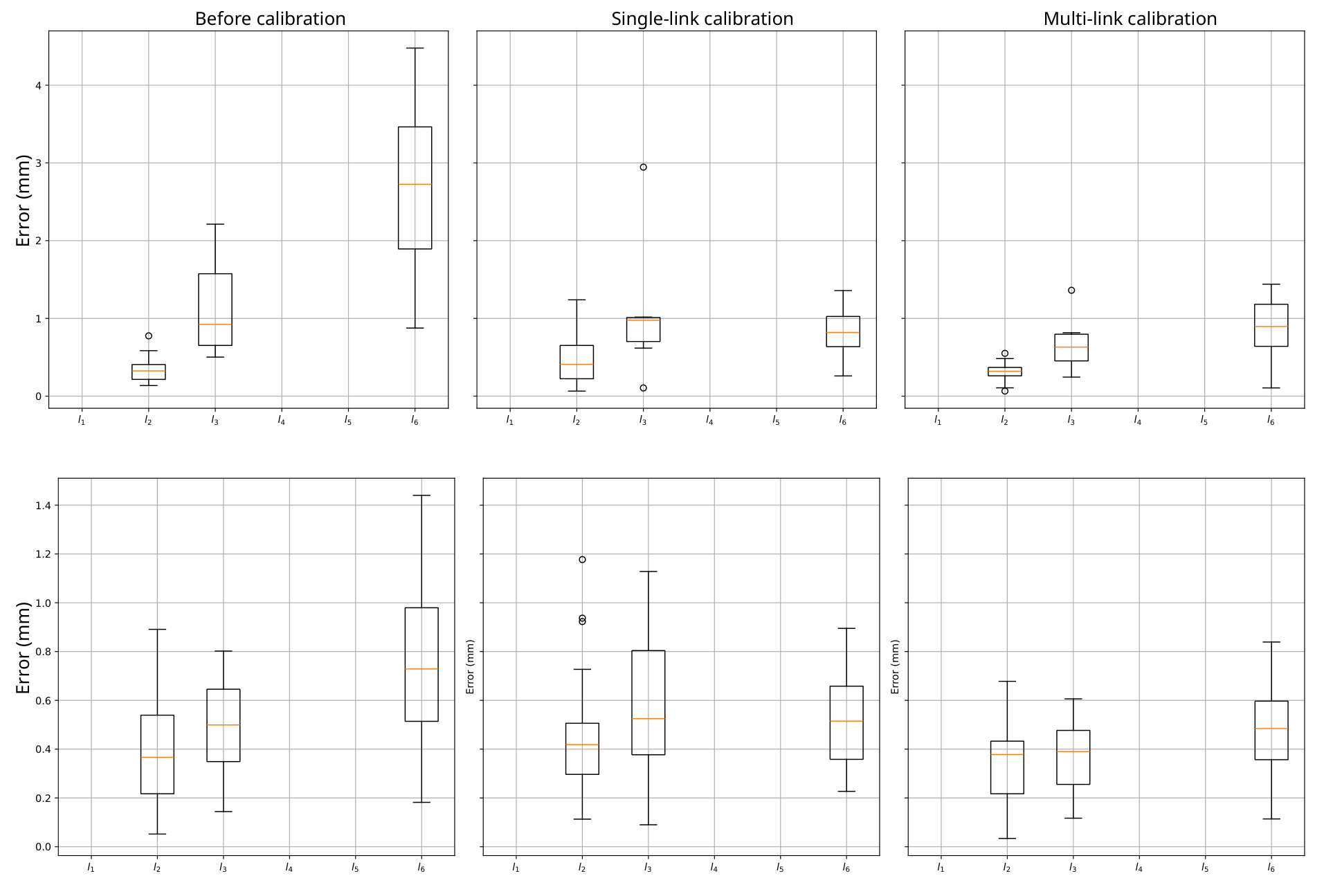
The resulting spatial residuals for both calibration approaches are presented in Figure 5.

For the demo robot (top row of Figure 5), both single- and multi-link calibration approaches demonstrate a roughly 3.5-fold improvement in the median residual compared with the default DH parameters from the manufacturer’s specifications (first column). Multi-link tracking provides a source of additional information: it allows observing how the kinematic model can diverge for intermediate links that were not explicitly included in the calibration objective. Strictly speaking, none of the above residuals are directly optimized as only validation residuals are demonstrated. But for the single-link approach, only end-effector used in optimization from the train set data. As seen for both robots (second column of Figure 5), the spatial residuals for Link 2 and Link 3 actually worsen with single-link calibration. Conversely, these residuals improve under the multi-link strategy. This degradation strongly indicates an overfitting problem within the single-link parameter identification. For the brand-new robot (bottom row of Figure 5), the overall improvement in median kinematic accuracy after calibration is less pronounced, decreasing from 0.74 mm (default) to 0.50 mm and 0.48 mm for single- and multi-link calibrations, respectively. Comparing the 99th percentile of kinematic residuals (the upper whisker) of the calibrated links, we observe that the error distribution is notably narrower for the multi-link approach for Link 2 and Link 3, indicating that this methodology provides more robust, consistent, and reliable calibration results overall.

To further evaluate the robustness of the calibration algorithms against poor initial estimates, an additional stress test was conducted on the demo robot dataset using the 50% training split. In this experiment, massive artificial uniform noise (up to 100 m in translation and ${360}^{\circ }$ in rotation) was intentionally injected into the predefined initial frame alignments, specifically the global base transform (${}^{w}M_b$) and the rigid cloud-to-link transforms (${}^{l_i}M_{c_i}$). The optimization process was restarted 30 times independently for both the single-link and multi-link problems. A run was considered successful if the Levenberg–Marquardt solver naturally converged based on the objective function variation threshold, rather than terminating prematurely due to an iteration limit. Under these severe initial distortions, the single-link calibration successfully converged in 66.7% of the cases (20 out of 30 trials). In contrast, the multi-link calibration demonstrated significantly higher sustainability, converging successfully in 76.7% of the trials (23 out of 30). This result suggests that observing multiple spatial constraints simultaneously widens the basin of attraction, making the multi-link optimization less prone to divergence even with highly inaccurate initial spatial constraints.

9. Conclusions

In this paper, a novel approach to the kinematic calibration of industrial robotic manipulators is presented. The study introduces a generalized objective function formulation for multi-link kinematic calibration utilizing photogrammetric pose tracking (10). By simulating the ROBOPRO RC-10 collaborative robot in the Blender3D environment (Figure 1), the authors evaluated the precision of the point cloud and link tracking backed by photogrammetry (Figure 3). Using custom calibration software built with machine learning-based automatic differentiation tools [31,32], simulation experiments successfully demonstrated the superior robustness and accuracy of the novel multi-link calibration strategy compared with traditional single-link approaches (Figure 4). The high potential of the new approach was further demonstrated through real experiments, confirming its enhanced numerical stability.