Article

Design of Dual-Motor Drive Composite Control Strategy Based on Iterative Learning Feedforward Control and Super-Twisting Sliding Mode Observer

1
School of Software, Shandong University, Jinan 250061, China
2
Key Laboratory of High Efficiency and Clean Mechanical Manufacture of Ministry of Education, Shandong University, Jinan 250061, China
3
School of Mechanical Engineering, Shandong University, Jinan 250061, China
*
Author to whom correspondence should be addressed.
Actuators 2026, 15(6), 343; https://doi.org/10.3390/act15060343
Submission received: 7 May 2026 / Revised: 12 June 2026 / Accepted: 14 June 2026 / Published: 17 June 2026
(This article belongs to the Section Control Systems)

Abstract

Periodic and non-periodic disturbances significantly affect the tracking accuracy of servo systems. A dual-motor drive composite control strategy based on iterative learning feedforward control and super-twisting sliding mode observer is proposed. Initially, a novel reaching law capable of dynamically adjusting gain coefficients based on system states is introduced, leading to the design of a sliding mode controller with proven asymptotic stability. To address non-periodic total disturbances, a super-twisting sliding mode observer is developed, and Lyapunov stability theory is employed to demonstrate system stability and error convergence to zero. A resonant controller is designed to suppress medium- to high-frequency periodic disturbances. For periodic total disturbances, a parameterized feedforward controller based on iterative learning is devised, and an input-shaping filter is introduced to refine the input trajectory. The feedforward control parameters are iteratively updated using a data-driven approach. Experiments are conducted on a differential dual-drive servo system. The nut motor adopts the sliding mode controller with an observer. The screw motor employs the iterative learning feedforward controller. Results show effective suppression of the disturbances. Speed ripple is reduced, and tracking accuracy is significantly improved. The study demonstrates the feasibility and advantage of combining robust control with iterative learning in high-precision servo systems.

1. Introduction

Servo feed systems based on permanent magnet synchronous motors (PMSMs) are widely applied in various ultra-precision instruments and equipment, such as high-end machine tools, 3D printers, and robots. Due to inherent structural characteristics, servo feed systems composed of PMSMs and ball screws inevitably suffer from nonlinear friction, backlash, vibration, deformation, and other influences. Moreover, PMSMs themselves are subject to nonlinear disturbances, parameter uncertainties, torque ripples, and other perturbations. These factors severely affect the tracking accuracy of servo feed systems and increase the difficulty of control [1,2].
Disturbances in servo feed systems can be classified into non-periodic disturbances and periodic disturbances. To mitigate the effects of non-periodic disturbances, high-performance algorithms have been continuously researched and improved by numerous scholars. An adaptive robust fault-tolerant controller based on a disturbance observer [3] was proposed for controlling dual-valve hydraulic systems. Yao [4] proposed an adaptive disturbance-observer-based composite control that estimates rotor imbalance and handles residual disturbances with unknown variation. Cui [5] embedded an adaptive fine disturbance observer into a PI controller using a second-order generalized integrator PLL but incurred high computational load and hardware demands. An online robust adaptive friction compensation scheme [6] enhances tracking at low speed and during zero-speed crossings and identifies parameters online without offline tests. And a neural-network-based finite-time command-filtered adaptive backstepping method [7] guarantees finite-time convergence and improves tracking. A proportional-integral adaptive robust controller based on a state equalizer [8] was used to reduce the impact of high-frequency disturbances on system stability. However, the speed closed-loop strategy of the state equalizer leads to a large phase lag.
Sliding mode control (SMC) remains a major focus. An adaptive terminal sliding mode reaching law based on continuous fast terminal sliding mode control [9] has been utilized to improve the speed control performance of PMSMs, achieving feedforward compensation of disturbances through a sliding mode disturbance observer. SMC is usually combined with disturbance observers. This combination [10] mitigates disturbance effects in speed regulation. Non-singular terminal sliding mode control methods [11,12] have been continuously optimized; by improving the scaling function, they avoid issues of unbounded gains and derivative singularities. Gao [13] introduced a high-gain observer that can effectively estimate system speed and acceleration, enhancing the system’s robustness and control accuracy.
Although the aforementioned highly robust controllers can effectively estimate and compensate for disturbances, their suppression performance on periodic disturbances is not ideal. For medium- and high-frequency periodic disturbances, a resonant controller [14] is a good choice. By connecting the resonant term in parallel with the feedback controller, suppression of medium- and high-frequency periodic disturbances is achieved.
Iterative Learning Control (ILC) is the most effective method for suppressing periodic disturbances, especially those related to absolute position and speed occurring under repetitive-motion conditions. A hybrid adaptive iterative learning sliding mode control method [15] can reduce the impact of periodic disturbances and suppress higher-order nonlinear disturbances. Iterative learning has been used to improve and optimize traditional high-gain observers; based on this, a fast integral terminal sliding mode hybrid control technique [16] was proposed. The introduction of iterative learning significantly enhanced the observer’s estimation accuracy for periodic disturbances. Iterative learning can also be combined with feedforward control [17]. An iterative feedforward tuning method [18] can eliminate the need for prior system knowledge in feedforward control and enhance the extrapolation capability of iterative learning. To reduce torque ripple, Huang [19] proposed a two-degree-of-freedom controller based on an extended sliding mode observer. Using a cascaded iterative learning design, it suppressed periodic disturbances while preserving dynamic response. Zhang [20] combined adaptive control and iterative learning for repetitive position tasks. By updating controller parameters using information from the previous cycle, the method effectively suppresses the influence of force ripples on speed tracking performance.
However, ILC improves the control performance of the current iteration cycle by learning from the control errors of previous iterations and requires the controlled system to have the same initial state each time it operates. This limitation means that ILC lacks the ability to compensate for non-repetitive disturbances. Therefore, ILC is usually employed as a feedforward control, combined with feedback control to achieve two-degree-of-freedom control. In the design of feedforward controllers based on ILC, it is usually necessary to know the precise Z-domain transfer function of the feedback controller, which implies that the feedback controller is linear. However, feedback controllers that can significantly suppress non-repetitive disturbances are usually nonlinear. This makes it difficult to combine the aforementioned highly robust feedback controllers with feedforward controllers based on ILC. To solve this problem, a composite control strategy integrating robust controllers and feedforward controllers is implemented on a differential dual-drive servo system [21,22]. Different control strategies are assigned to the two actuators of a differential dual-drive servo system based on their disturbance characteristics. Existing methods based on STSMO primarily enhance the robustness of a single feedback loop by estimating total disturbances, but their effectiveness in compensating for repetitive periodic errors is limited. Meanwhile, existing feedforward approaches based on ILC can effectively reduce periodic tracking errors during repetitive motions, yet they typically require co-design with linear feedback controllers and depend on precise closed-loop transfer functions—a requirement that restricts their direct integration with nonlinear robust controllers such as SMC. In contrast, the proposed hybrid strategy leverages the dual-motor structure itself as a control decoupling mechanism, thereby avoiding these conflicts. The nut motor is controlled by an STSMO-SMC to suppress non-periodic and time-varying disturbances in real time, while the screw motor employs a parameterized ILFFC to learn and compensate for repetitive periodic disturbances. Thus, this method provides a practical approach to integrating nonlinear robust feedback control with iterative learning feedforward compensation in high-precision dual-motor servo systems.
Based on the transmission mechanism and advantages of the differential dual-drive servo system, this paper further studies the high-performance servo control algorithm to achieve high-precision position tracking performance. The main contributions of this paper are summarized as follows:
(1)
A disturbance-oriented composite control framework is proposed for the differential dual-drive servo system. Unlike conventional dual-motor schemes that apply similar control laws to both motors, the proposed method assigns different disturbance-suppression tasks to two actuators. The nut motor is responsible for robust real-time suppression of non-periodic disturbances, and the screw motor is responsible for iterative compensation of repetitive periodic disturbances.
(2)
A super-twisting sliding mode observer is designed for the nut motor to suppress the non-periodic total disturbance, and an SMC based on the improved new reaching law is proposed. Through Lyapunov theory, it is proven that the control system is asymptotically stable, the error is bounded and the convergence is zero.
(3)
A parametric feedforward controller based on an input-shaping filter is designed for the screw motor. The parameters are optimized iteratively in the process of iterative learning by a data-driven method.
The remainder of this paper is organized as follows. Section 2 introduces the operating principle of the differential dual-drive servo system and analyzes the disturbance-suppression problem. Section 3 designs a sliding mode controller with a new reaching law and a super-twisting sliding mode observer. Section 4 proposes a parameterized feedforward controller with an input-shaping filter. Section 5 reports the experimental validation.
The complete nomenclature is shown in Table 1.

2. Differential Dual-Drive Servo System Model and Problem Statement

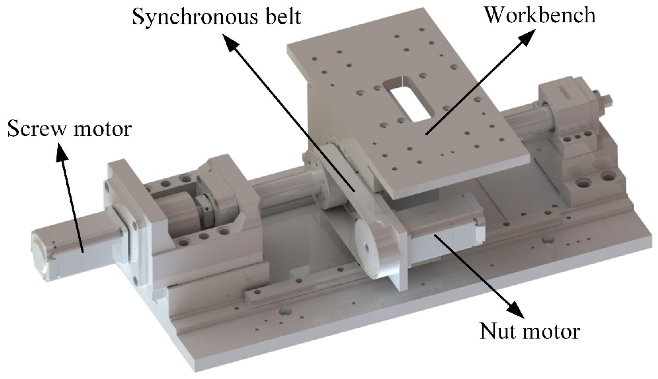
The differential dual-drive servo system is shown in Figure 1. It is a new type of feed system in which both the screw and the nut can be rotated. The screw motor directly drives the screw to rotate through the coupling, and the nut motor drives the nut to rotate through the synchronous belt. The rotation directions of the two are the same, and the synthesized speed is the feed speed of the table. The speed of the two motors is higher than the critical speed of the crawling phenomenon, avoiding the low-speed creeping area of the motor. The workbench can move uniformly at an extremely low speed without a crawling phenomenon. Compared with the traditional servo system, the differential dual-drive servo system significantly improves low-speed performance, reduces tracking error, and can achieve higher precision feed and positioning. However, since the speed of the workbench is synthesized by the speed of two motors, this leads to an increase in the disturbance and vibration sources of the system. All kinds of interference of the two motors are mapped to the worktable, which affects the tracking accuracy of the worktable. Therefore, it is very important to suppress the disturbance of the two motors to improve the control performance of the system.
The screw drive shaft and nut drive shaft in the differential dual-drive servo system are both PMSM-based servo systems. Therefore, the research object of this paper can be regarded as a servo feed system based on a permanent magnet synchronous motor. In order to facilitate the subsequent mathematical model establishment and related controller design, the following assumptions are first made for PMSM:
(1)
The magnetic core is unsaturated, that is, the magnetic circuit saturation is ignored;
(2)
The three-phase windings are symmetrically distributed, and the axes of each winding are 120 degrees apart in space;
(3)
The core permeability is infinite, ignoring the eddy current loss and hysteresis loss of the stator and rotor core;
(4)
Constant winding resistance and inductance;
(5)
The end effect and alveolar effect are ignored.
Based on the above assumptions, in the synchronous rotating reference frame, the dq axis voltage equation can be expressed as
u d = R i d + L d d i d d t ω e L q i q u q = R i q + L q d i q d t + ω e ( L d i d + ψ f )
In the equation, u d and u q are the d-axis and q-axis voltages, i d and i q are the d-axis and q-axis currents, R is the stator winding resistance, L d and L q are the d-axis and q-axis inductances, ψ f is the permanent magnet flux linkage, ω e = n P ω m , ω e is the rotor electrical angular velocity, n P is the pole pair, and ω m is the rotor mechanical angular velocity.
According to Newton’s second law, the dynamic equation of PMSM can be expressed as
J ω ˙ m = T e B ω m T L
where T e is the electromagnetic torque, J is the moment of inertia of the motor, B is the damping viscosity coefficient, and T L is the load torque.
Using magnetic field-oriented control, when the d-axis current is zero, the output torque reaches the maximum. For PMSM, the d-axis inductance is equal to the q-axis inductance, that is, L d = L q = L , and the electromagnetic torque T e can be expressed as
T e = 3 2 n p i q [ i d ( L d L q ) + ψ f ] = 3 2 n p ψ f i q = K t i q
where K t is the torque coefficient.
Equation (2) represents the dynamic equation of the PMSM derived under ideal conditions, ignoring the influence of various disturbances on the motor’s operational performance. However, under practical operating conditions, the PMSM servo feed system is subjected to various internal and external disturbances. For example, nonlinear friction is generated at the contact surfaces of mechanical transmission components such as ball screw–nut pairs and guide rails. Torque ripples are induced by end effects and cogging effects. Parameter uncertainties arise from unmodeled system dynamics and inaccurate parameter identification. Additionally, unknown disturbances originate from the external environment. Combined with Equation (3), Equation (2) is further modified as
( J + Δ J ) ω ˙ m = ( K t + Δ K t ) i q ( B + Δ B ) ω m T L T f
where Δ J is the deviation between the identified value and the actual value of the moment of inertia, Δ K t is the deviation between the theoretical value and the actual value of the torque coefficient, Δ B is the uncertainty of the damping viscosity coefficient, and T f is the external total disturbance.
Equation (4) can be expressed as
J ω ˙ m = K t i q B ω m T ω T r
where T r = T r L + T r f + Δ B ω m + Δ J ω ˙ m Δ K t i q denotes non-periodic total disturbances, primarily including non-repeating external load torques T r L , friction changes T r f caused by temperature rise, contact condition changes and parameter uncertainties Δ B ω m ,   Δ J ω ˙ m ,   Δ K t i q . Periodic total disturbances are represented by T ω . They refer to disturbances that exhibit periodic variations or repetitive disturbances with fixed relationships to absolute position and speed. Examples of periodic disturbances include flux-linkage harmonics generated by PMSMs, current sampling errors, inverter nonlinearities, and cogging torque. Additionally, under repetitive-motion conditions, disturbances related to absolute position and speed, such as ball screw manufacturing errors and installation backlash, are also considered periodic disturbances.
For the system represented by (5), the state space equation can be further expressed as
J x ˙ 1 = K t u B x 1 T ω T r x ˙ 2 = x 1 y = x
where x = [ x 1 , x 2 ] T , x 1 = ω m , x 2 = θ m , u is the control quantity of the system, u = i q , and y is the output of the system.
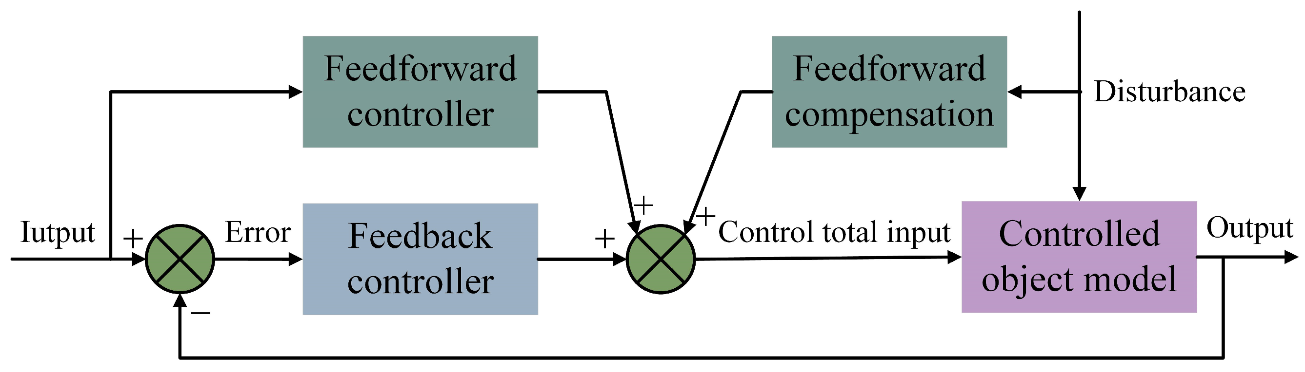
The ultra-precision servo motion control based on PMSM generally adopts a two-degree-of-freedom control structure combining feedback control and feedforward control, as shown in Figure 2. The feedback controller can achieve high-precision trajectory tracking, suppress disturbance and reduce tracking error. However, the error source cannot be completely compensated, and the suppression ability will be limited by the modal of the mechanical structure. The feedforward controller can compensate for the trajectory error and external disturbance in time on the basis of feedback control to stabilize the closed-loop system and further improve the response speed and motion accuracy of the system.
The aperiodic total disturbance and periodic total disturbance in Equation (6) will eventually be mapped to the servo feed motion of the workbench. In order to reduce the influence of various disturbances on the performance of the servo system, on the one hand, a disturbance observer can be designed to estimate the disturbances and feed them back to the controller for compensation. On the other hand, the disturbances can be approximated and compensated by iterative learning. However, this method requires that the disturbances are periodic. For the servo feed system of high-precision machine tools, there are a large number of working conditions in which the reference trajectory is completely repeated, which will produce periodic disturbances related to the absolute position. Moreover, the cogging torque, flux harmonics and current measurement errors of the motor will also cause the PMSM to generate harmonic torque, causing periodic disturbances. Compared with the disturbance observer, the iterative learning method has a better compensation effect on periodic disturbances. Therefore, in order to achieve a better suppression effect on the disturbances, it is necessary to design relevant algorithms to suppress the aperiodic and periodic total disturbances, respectively.
The parametric feedforward controller based on iterative learning is used as the feedforward control of the two-degree-of-freedom control structure to achieve effective suppression of periodic disturbances. However, in the design of a feedforward controller, it is required to know the exact z-domain transfer function of the feedback controller, which requires the feedback controller to be linear, such as the common PI controller. However, the robust performance of such control schemes is poor, and it is difficult to suppress non-repetitive disturbances in time. Feedback controllers with high robustness, such as adaptive controllers and sliding mode controllers, are usually nonlinear. Such controllers cannot be described by accurate transfer functions, so they are difficult to use as feedback controllers in two-degree-of-freedom control structures.
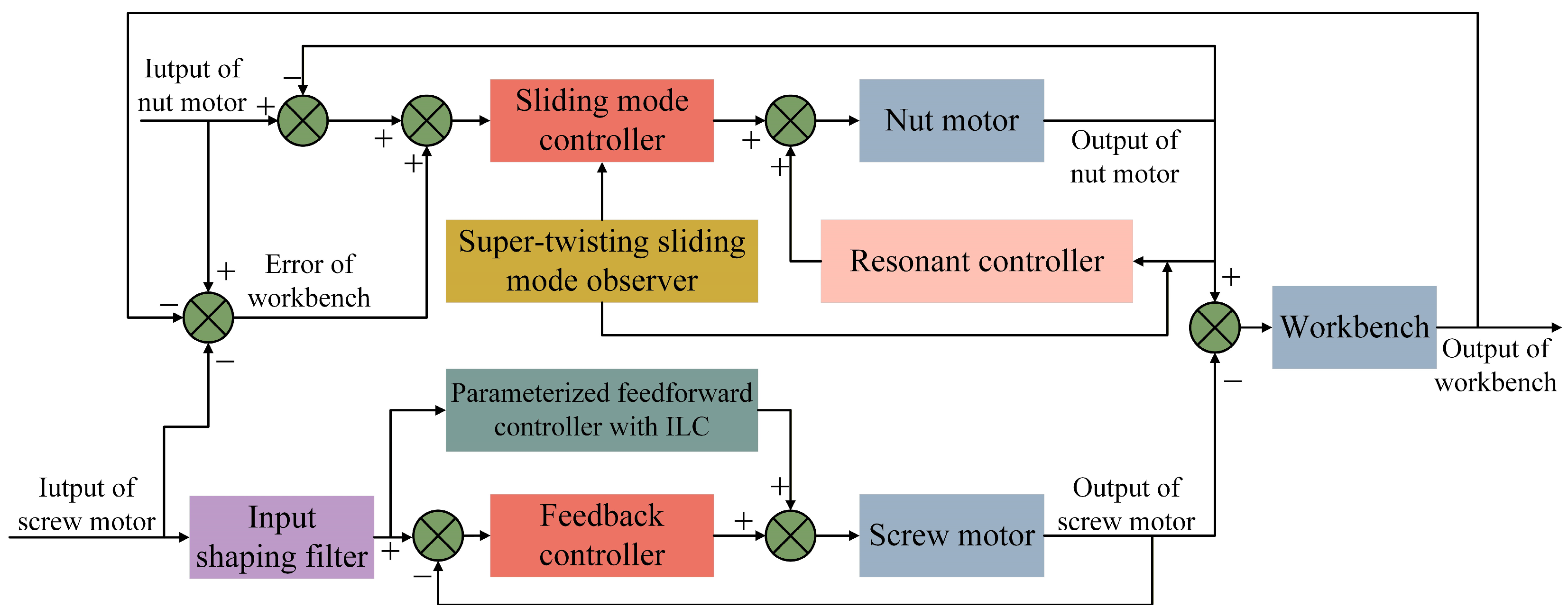
In order to solve this problem, the dual-motor drive composite control strategy is proposed as shown in Figure 3. In the differential dual-drive servo system, the nut motor adopts a sliding mode controller based on the super-twisting sliding mode observer. The non-periodic disturbances and non-repetitive time-varying disturbances of the workbench are fed back to the nut motor to suppress and improve the robust performance of the system. The screw motor adopts a parametric feedforward controller based on iterative learning. The periodic disturbance of the workbench is feedforward-compensated by the screw motor, and the tracking accuracy is continuously improved through iterative learning. Through the above scheme, the parametric feedforward controller and the high robustness feedback controller can be combined and used for the control of the servo feed table. It not only suppresses the periodic disturbance but also reduces the speed fluctuation. It ensures the high-precision motion control of the system, takes into account the robustness of the system, and can achieve timely and effective suppression of time-varying aperiodic disturbances. Therefore, this paper designs two controllers to reduce speed fluctuation and improve feed accuracy.

3. Design of Sliding Mode Controller Based on Super-Twisting Sliding Mode Observer

3.1. Design of Sliding Mode Controller Based on New Reaching Law

In order for the sliding mode controller to converge and effectively track the system trajectory, the sliding mode reaching condition must be satisfied
s s ˙ < 0
where s is the sliding surface. The key to the design of the sliding mode controller is the design of the sliding mode surface and the design of the reaching law. An appropriate reaching law can effectively reduce the chattering of the system.
The tracking error of the system is defined as e m = x r x 1 , and x r = ω r is the desired angular velocity. The sliding surface is further designed as follows
s = k e m + p 0 t e m d t
where k is the proportional coefficient and p is the integral coefficient. k > 0 and p > 0 .
Derivation of Equation (8) can be obtained as follows
s ˙ = k e ˙ m + p e m
In this section, the influence of the periodic total disturbance in Equation (6) on the system is temporarily ignored and substituted into Equation (8).
s ˙ = k K t J u + k B J x 1 + k J T r + k x ˙ r + p e m
Equation (10) can be interpreted as the dynamic expression of the sliding surface. s = 0 defines the motion of the system staying on the sliding surface. A new reaching law is further designed to make the system converge to zero in finite time and minimize the adverse effects of chattering on system performance. The reaching law is designed as follows
s ˙ = ζ ( e m , s ) s i g m o i d ( s )
where ζ ( e m , s ) < 0 is a variable gain coefficient that can suppress the chattering phenomenon, which can be expressed as
ζ ( e m , s ) = c e δ s ε + ( 1 + 1 e m 2 ε ) e δ s
where c is the control gain, c > 0 , δ is the exponential decay rate, δ > 0 , 0 < ε < 1 , and the value of ε affects the degree of system chattering and the length of convergence time. According to the analysis of Equation (12), when s increases, that is, when the system is far away from the sliding mode surface, e δ s tends to zero and e δ s > 1 and increases with the increase of s . ζ ( e m , s ) tends to c e δ s ε . It can be seen that the absolute value of the gain coefficient variable is greater than the control gain, and the value increases with the increase of s . This means that when the system is far away from the sliding mode surface, it will obtain greater gain, so that the system can reach the sliding mode surface at a faster speed and shorten the convergence time. When s decreases, that is, when the system is close to the sliding mode surface, e δ s and e δ s tend to one, ζ ( e m , s ) tends to c e m 2 e m 2 + 1 , and the system tracking error e m gradually decreases and tends to zero, which means that the variable gain coefficient tends to zero, which can reduce the chattering of the system. Therefore, the reaching law can dynamically adjust the variable gain coefficient according to the system state to achieve better control performance.
Using the function shown in Equation (13) instead of the sign function can effectively reduce the system chattering.
s i g m o i d ( s ) = 2 1 + e s 1
Combined with Equations (10) and (11), the control quantity of the system is designed as follows
u = B K t x 1 + 1 K t T r + J K t x ˙ r + J k K t p e m J k K t ζ ( e m , s ) s i g m o i d ( s )
The non-periodic total disturbances T r will subsequently design an observer to estimate its size.
Theorem 1.
The system described in Equation (6) is asymptotically stable, and the error converges to zero.
Proof. 
Define the Lyapunov function as
V 1 = 1 2 s 2
Taking the derivative of Equation (15), it follows that
V ˙ 1 = s s ˙
Combining Equations (10), (11) and (14), we can further obtain
V ˙ 1 = s ζ ( e m , s ) s i g m o i d ( s )
It is known that ζ ( e m , s ) < 0 , when s > 0 , s i g m o i d ( s ) > 0 , then V ˙ 1 < 0 ; when s 0 , s i g m o i d ( s ) 0 , then V ˙ 1 0 . Therefore, V ˙ 1 0 ; the system is asymptotically stable. That is, s 0 , s ˙ 0 . Furthermore, it follows that
k e m + p 0 t e m d t = 0
Take the derivative of (18) to get
k e ˙ m + p e m = 0
By solving the linear differential equation, it follows that
e m = e m ( t 0 ) exp ( p k ( t t 0 ) )
where t is the time and t 0 is the initial time. As the time t increases, the tracking error e m gradually approaches zero. Therefore, both the sliding variable s and the tracking error e m asymptotically converge to zero. Hence, the system is asymptotically stable. Theorem 1 is proven. □

3.2. Design of Super-Twisting Sliding Mode Observer for Non-Periodic Total Disturbances

The aperiodic disturbances will seriously affect the motion accuracy of the servo feed system. It is necessary to design a disturbance observer that can observe and compensate for the aperiodic disturbances in real time. Compared with the traditional extended state observer, the observer based on sliding mode control theory has better adaptability and robustness. Sliding mode control based on the super-twisting algorithm is a kind of second-order sliding mode control, which can effectively solve the chattering problem of traditional sliding mode control and has better control performance.
In the permanent magnet synchronous motor servo feed system, the sampling frequency of the position loop and the speed loop is much higher than the change frequency of the disturbances, which means that the change in the disturbances is very slow in a single control period. Therefore, it is assumed that the disturbance derivative is bounded and sufficiently slow-varying within one sampling period. The expanded expression of system (6) is
x ˙ 1 = B J x 1 1 J T r + K t J u
Define the integral sliding surface s o b as
s o b = e o b + c o b 0 t e o b d t
where c o b is the integral constant, e o b is the observation error, and e o b = ω m ω ^ m = x 1 x ^ 1 .
Furthermore, the super-twisting sliding mode observer is designed in the following form
x ^ ˙ 1 T ^ ˙ r = B J 1 J 0 0 x ^ 1 T ^ r + K t J 0 u + w ( s o b ) v ( s o b )
where x ^ 1 is the observation value of the system state variable, T ^ r is the observation value of the non-periodic integrated total disturbances, and w ( s o b ) and v ( s o b ) are the sliding mode control laws. Based on the super-twisting algorithm, the sliding mode control law is designed as follows
w ( s o b ) = ( c o b B J ) e o b + λ s o b 1 2 sgn ( s o b ) v ( s o b ) = α sgn ( s o b )
where α and λ is the observer gain and α > 0 , λ > 0 . sgn ( ) is a symbol function.
The error of the super-twisting sliding mode observer can be obtained by subtracting Equation (21) from Equation (23)
e ˙ o b e ˙ o r = 0 T ˙ r + B J 1 J 0 0 e o b e o r + w ( s o b ) v ( s o b )
where e o r = T r T ^ r .
Theorem 2 ([23]).
Given that the first-order derivative of the total disturbance T ˙ r is bounded, there exists a constant ρ such that 1 J T ˙ r ρ . If the observer parameters satisfy λ > 2 and α J > λ 2 + 4 ρ 2 4 ( λ 2 ) , then the observer error converges to zero in finite time, and the observer is stable.
Proof. 
Take the derivative of Equation (22) to get
s ˙ o b = e ˙ o b + c o b e o b
Combining Equations (24) and (25) yields
s ˙ o b = λ s o b 1 / 2 sgn ( s o b ) + η
where η = 1 J e o r . And its derivative is
η ˙ = 1 J ( c v ( s o b ) ) = α J sgn ( s o b ) + Δ ( t )
where Δ ( t ) = 1 J T ˙ r and
Δ ( t ) ρ
Define the auxiliary vector ξ as
ξ = ξ 1 ξ 2 = = s o b 1 / 2 sgn ( s o b ) η
From Equation (30), it can be known that s o b = ξ 1 ξ 1 , s ˙ o b = 2 ξ 1 ξ ˙ 1 . According to Equation (27), we can obtain 2 ξ 1 ξ ˙ 1 = λ ξ 1 + ξ 2 . The state dynamics can be expressed as
ξ ˙ 1 = 1 ξ 1 ( λ 2 ξ 1 + 1 2 ξ 2 )
ξ ˙ 2 = 1 ξ 1 ( α J ξ 1 + ξ 1 Δ ( t ) )
Combining Equation (30), the following is obtained
ξ ˙ = 1 ξ 1 ( A ξ + B φ )
where A = λ 2 1 2 α J 0 , B = 0 1 , and φ = ξ 1 Δ ( t ) . According to Equation (29), the following is obtained
φ 2 ρ 2 ξ 1 2
In order to analyze the stability of the super-twisting sliding mode observer, the following Lyapunov function is defined as
V 2 = ξ T P ξ
where P = 1 2 λ 2 + 4 α J λ λ 2 . Since P is a symmetric positive definite matrix, there exist positive numbers P min and P max such that
P min ξ 2 2 V 2 P max ξ 2 2
where 2 denotes the Euclidean norm of a vector. Take the derivative of Equation (35) to get
V ˙ 2 = 1 ξ ξ φ T A T P + P A P B B T P 0 ξ φ
According to Equation (34), ρ 2 ξ 1 2 φ 2 0 . Therefore,
V ˙ 2 1 ξ ξ φ T A T P + P A + ρ 2 C P B B T P 1 ξ φ 1 ξ ξ T Q ξ
where Q = ( A T P + P A + ρ 2 C + P B B T P ) = 1 2 λ 3 1 2 λ 2 + 2 λ α J 2 ρ 2 λ 2 + λ λ 2 + λ λ 2 . If Q is a positive definite matrix, the following conditions hold.
λ 2 > 0 ( λ 3 1 2 λ 2 + 2 λ α J 2 ρ 2 ) ( λ 2 ) ( λ 2 + λ ) 2 > 0
So, λ > 2 , α J > λ 2 + 4 ρ 2 4 ( λ 2 ) . Under these conditions, Q is a positive definite matrix, and there exists a positive number Q min such that
ξ T Q ξ Q min ξ 2 2
Combining Equation (38), it follows that
V ˙ 2 Q min ξ 1 ξ 2 2 ζ V 2
where ζ = Q min P max > 0 .
Therefore, when λ > 2 and α J > λ 2 + 4 ρ 2 4 ( λ 2 ) , V ˙ 2 ζ V 2 . According to the finite-time stability theory [23], it follows that ξ 1 and ξ 2 converge to zero within a finite time, that is, the disturbance observation error e o r converges to zero within a finite time, and the system is stable. Theorem 2 is proven. □

3.3. Design of Resonant Controller for Medium- and High-Frequency Periodic Disturbances

The super-twisting sliding mode observer designed in the previous section can effectively observe and compensate for non-periodic disturbances. In fact, it also has a certain suppression effect on periodic disturbances with a lower frequency. However, the feedback control based on the super-twisting sliding mode observer cannot fully compensate for the influence of periodic disturbances on control accuracy. Especially for high-frequency periodic disturbances such as electrical disturbances and harmonic torques, the observer has little effect on their suppression. The resonant controller and the observer-based feedback control are designed in parallel to further suppress the influence of high-frequency periodic disturbances on velocity fluctuation and positioning accuracy.
The transfer function of the resonant controller is usually expressed as
G r c ( s ) = κ s s 2 + ω 0 2
where ω 0 is the resonant frequency and κ is the gain of the resonant controller. By introducing the adjustable phase angle term φ r , the stability of the resonant controller is improved, and Equation (42) is further optimized to be
G r c ( s ) = κ ( s cos φ r ω 0 sin φ r ) s 2 + ω 0 2
The resonant controller has a good suppression effect mainly for high-frequency periodic disturbances. The high-frequency disturbance of the servo AC motor mainly comes from the electrical part, such as current sampling error, inverter nonlinearity and flux-linkage harmonics. The periodic disturbances caused by inverter nonlinearity and flux harmonics are small, and the related compensation algorithm needs to be completed in the current loop. The designed resonant controller mainly suppresses the disturbances caused by the current sampling error. Other periodic disturbance components that are not compensated will be further addressed in the iterative feedforward method in the future.
The torque error caused by current sampling makes the output torque have the same harmonic component, which further leads to speed fluctuation at the same frequency. The torque error caused by direct current bias can be expressed as
Δ T 1 = K f o 2 3 Δ i a _ d c 2 + Δ i a _ d c Δ i b _ d c + Δ i b _ d c 2 cos ( ω e t + φ e )
The torque error caused at frequency 2 ω e can be described as
Δ T 2 = S a S b S a S b K f o i 3 cos ( 2 ω e + π 3 ) + S a S b S a S b K f o i 2 3
where S a and S b are proportional factors, which will cause the output torque to produce the same frequency of torque harmonics at 2 ω e .
From Equations (44) and (45), it can be seen that the current sampling error will introduce the torque harmonic component, whose frequency is the sum, which can be equivalent to the periodic disturbance of the position loop and the speed loop. According to the above analysis, the resonant controller is designed as follows
G r c 1 ( s ) = κ 1 ( s cos φ r 1 ω e sin φ r 1 ) s 2 + ω e 2
G r c 2 ( s ) = κ 2 ( s cos φ r 2 2 ω e sin φ r 2 ) s 2 + ( 2 ω e ) 2
By connecting the above resonant controller in parallel with the feedback controller, the periodic disturbances can be effectively suppressed, thereby reducing the speed fluctuation under steady state.

4. Design of Feedforward Controller Based on Iterative Learning

The sliding mode controller based on the super-twisting sliding mode observer and the parallel resonant controller can suppress the non-periodic disturbances and the periodic disturbances in the finite frequency range, but there are still some periodic disturbances that have not been suppressed. Feedforward control based on iterative learning is one of the best methods to suppress periodic disturbances. The control scheme of iterative feedforward is realized on the screw motor. By learning the control error of the previous iteration period of the workbench, the control performance of the uncompensated periodic disturbance’s residual component in the current iteration period can be effectively improved.

4.1. Parameterized Feedforward Controller Based on Input-Shaping Filter

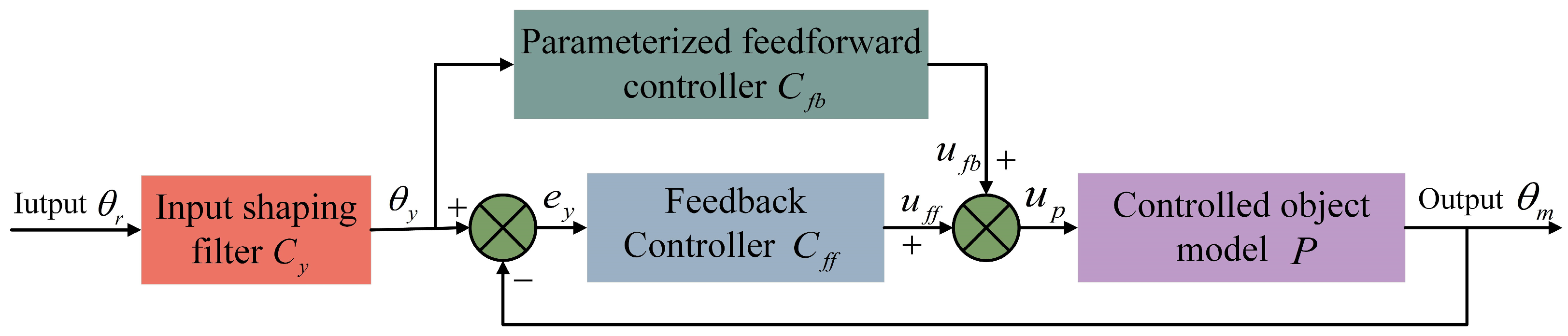
The two-degree-of-freedom control block diagram including the input-shaping filter and the parameterized feedforward controller is shown in Figure 4. The feedforward controller adopts the parameterized feedforward control method and updates the parameters of the feedforward controller by iterative feedforward tuning.
In Figure 4, C y is the input-shaping filter, C f f is the parameterized feedforward controller, C f b is the feedback controller, P is the controlled object, θ r is the desired input trajectory signal, θ y is the input trajectory signal after shaping, e y is the trajectory tracking error, u f f is the feedforward control signal, u f b is the feedback control signal, u p is the integrated control signal, and θ m is the system output trajectory signal. By introducing the basis function, the input-shaping filter and the feedforward controller can be expressed as
Ω = ( C y , C f f ) | C y = A ( z 1 , θ ) ,   C f f = B ( z 1 , θ ) ,   θ R n a + n b
By parameterizing the input-shaping filter and the feedforward controller based on the polynomial basis function FIR filter, then
A ( z 1 , θ ) = 1 + i = 1 n a φ i ( z 1 ) θ i
B ( z 1 , θ ) = i = n a + 1 n a + n b φ i ( z 1 ) θ i
where θ is the feedforward controller parameter, θ = [ θ 1 , θ 2 , , θ n a , , θ n a + n b ] T , φ is the basis function vector, and φ = [ φ 1 , φ 2 , , φ n a , φ n a + n b ] .
In the (k + 1)th iteration, the input-shaping filter and the feedforward controller are iteratively updated based on the iterative learning theory, and the update formula can be expressed as
C y k + 1 = C y k + C y Δ = 1 + i = 1 n a φ i ( z 1 ) θ i k + i = 1 n a φ i ( z 1 ) θ i Δ
C f f k + 1 = C f f k + C f f Δ = i = n a + 1 n a + n b φ i ( z 1 ) θ i k + i = n a + 1 n a + n b φ i ( z 1 ) θ i Δ
where θ Δ is the parameter variation in the current iteration period, θ Δ = [ θ 1 Δ , θ 2 Δ , , θ n a Δ , , θ n a + n b Δ ] T .
According to Equations (51) and (52), after the basis function φ is determined, it is also necessary to obtain the iterative update law of the parameter θ . The objective function is usually defined as J o b = e 2 2 , and the least squares method and gradient descent method are used to solve the parameter update law. However, the parameter θ obtained in this way is unconstrained. When its variation is too large, it may cause the feedforward control signal to be too large, which in turn causes the control signal to exceed the signal output range and seriously deteriorate the performance of the system. Therefore, it is necessary to constrain the control signal and its variation.
Firstly, the tracking error is defined as
e y = θ y θ m
Without considering the interference, the expressions of the shaped input trajectory signal θ y k and the tracking error e y k obtained by the kth iteration are
θ y k = θ r C y k
e y k = θ y k θ m k
According to the system block diagram, the system output signal, control signal and error of the kth iteration can be expressed as
θ m k = S P ( C f b C y k + C f f k ) θ r
u k = S ( C f b C y k + C f f k ) θ r
where S is the system closed-loop sensitivity function, which is defined as S = ( 1 + P C f b ) 1 . S P represents the transfer relationship from equivalent control input to output. The sensitivity function C 0 is defined as
C 0 = C f b C y + C f f
S and SP are highly correlated with system model parameters. The data-driven method is used to eliminate the dependence of S and SP on the model. Equations (56) and (57) can be rewritten as
S P θ r = C 0 1 θ m k
S θ r = C 0 1 u k
The error e y k of the kth iteration can be expressed as e y k = S ( C y k P C f f k ) θ r . Combining Equations (59) and (60) can yield
e y k = C y k C 0 1 u k C f f k C 0 1 θ m k

4.2. Iterative Parameter Update Based on a Data-Driven Method

In order to control the amplitude of the control parameter variation θ Δ and prevent the control signal from exceeding the execution range of the motor, the optimal iterative feedforward parameter algorithm is adopted, and the control parameters are iteratively updated by a data-driven method. The control signal and its variation are directly constrained, and the new objective function is defined as
J o b = e y 2 2 + ρ 1 u 2 2 + ρ 2 Δ u 2 2
where ρ 1 and ρ 2 are the constraint coefficients of the control signal u and the control signal variation Δ u , respectively. Based on the data-driven theory, according to the kth iteration data, the objective function (62) should be minimized at the (k + 1)th iteration, that is
min J o b = min e y k + 1 2 2 + ρ 1 u k + 1 2 2 + ρ 2 Δ u k + 1 2 2
According to Equations (57) and (61), the expression of the relevant variables can be obtained as follows
e y k + 1 = e y k + S ( C y Δ P C f f Δ ) = e y k + C y Δ C 0 1 u k C f f Δ C 0 1 θ m k
u k + 1 = u k + S ( C f b C y Δ + C f f Δ ) θ r = u k + ( C f b C y Δ + C f f Δ ) C 0 1 u k
Δ u = ( C f b C y Δ + C f f Δ ) C 0 1 u k
The partial derivative of Equation (61) can be obtained as follows
e y k θ k = C y k θ k C f f k θ k C 0 1 u k θ m k = φ C 0 1 u k θ m k
Let w D = φ C 0 1 u k θ m k ; w D denotes the influence matrix of feedforward parameter variations on the tracking error in the next iteration. Then we can obtain
e y k + 1 = e y k w D θ Δ
u k + 1 = u k + w L θ Δ
Δ u = w L θ Δ
where w L = [ C f b φ 1 , , C f b φ n a , φ n a + 1 , , φ n a + n b ] C 0 1 u k . w L represents the influence matrix of feedforward parameter variations on the control input and its increment. Then the objective function can be expressed as
J o b = ( e y k w D θ Δ ) T ( e y k w D θ Δ ) + ρ 1 ( u k + w L θ Δ ) T ( u k + w L θ Δ ) + ρ 2 ( w L θ Δ ) T ( w L θ Δ )
Let the objective function take the minimum value, and let its derivative be zero; then we can obtain
J Δ θ = 2 w D T ( e y k w D θ Δ ) + 2 ρ 1 w L T ( u k + w L θ Δ ) + 2 ρ 2 w L T w L θ Δ = 0
According to Equation (72), we can obtain
θ Δ = [ w D T w D + ( ρ 1 + ρ 2 ) w L T w L ] 1 ( w D T e y k ρ 1 w L T u k )
It can be seen from Equation (73) that by setting the values of parameters ρ 1 and ρ 2 , the size of parameter variation θ Δ is directly constrained, which affects the convergence speed and value range of feedforward controller parameter θ . Further, indirectly limiting the size of the control signal and its variation can effectively prevent the control performance instability caused by the excessive control signal.
Feedforward control can effectively suppress periodic disturbances so that the tracking error and speed fluctuation are continuously reduced. The input-shaping filter can suppress vibration and smooth the trajectory without reducing the overall performance of the system. In addition, the parametric feedforward controller and input-shaping filter will not affect the stability of the whole system.

4.3. Algorithm Procedure

The algorithm procedure of the Optimal iterative feedforward parameter algorithm is shown in Algorithm 1. In the first iteration cycle, the initial values of the parameterized feedforward controller and the input-shaping filter are both zero; that is, only the feedback controller is used to carry out the closed-loop experiment. The system output signal and other related data of the first cycle are collected, and the feedforward controller and the input-shaping filter for the next cycle are updated. With the increase in the iteration cycle, the tracking error of the reference trajectory decreases continuously.
Algorithm 1. Optimal iterative feedforward parameter algorithm
  • Select the appropriate basis function φ , and give the appropriate initial value to the parameter vector θ to be identified;
  • Initialize parameterized feedforward controller C f f and input-shaping filter C y ;
  • Initialize the constraint coefficients ρ 1 and ρ 2 , and set the values of e y 1 , u 1 and θ m 1 to 0;
  • for each step, k = 1, 2, …, k max , do
  • The closed-loop experiment of the system is carried out, and the output signal θ m k , control signal u k and error signal e y k of the system are collected;
  • Calculate the values of w D and w L in the current iteration period. w D = φ C 0 1 u k θ m k , w L = [ C f b φ 1 , , C f b φ n a , φ n a + 1 , , φ n a + n b ] C 0 1 u k ;
  • Calculate the variation of parameter θ , θ Δ = [ w D T w D + ( ρ 1 + ρ 2 ) w L T w L ] 1 ( w D T e y k ρ 1 w L T u k ) ;
  • Update the parameterized feedforward controller C f f k + 1 and input shaping filter C y k + 1 for the next cycle;
  • end for.

5. Experimental Verification

5.1. Experimental Equipment and Parameter Setting

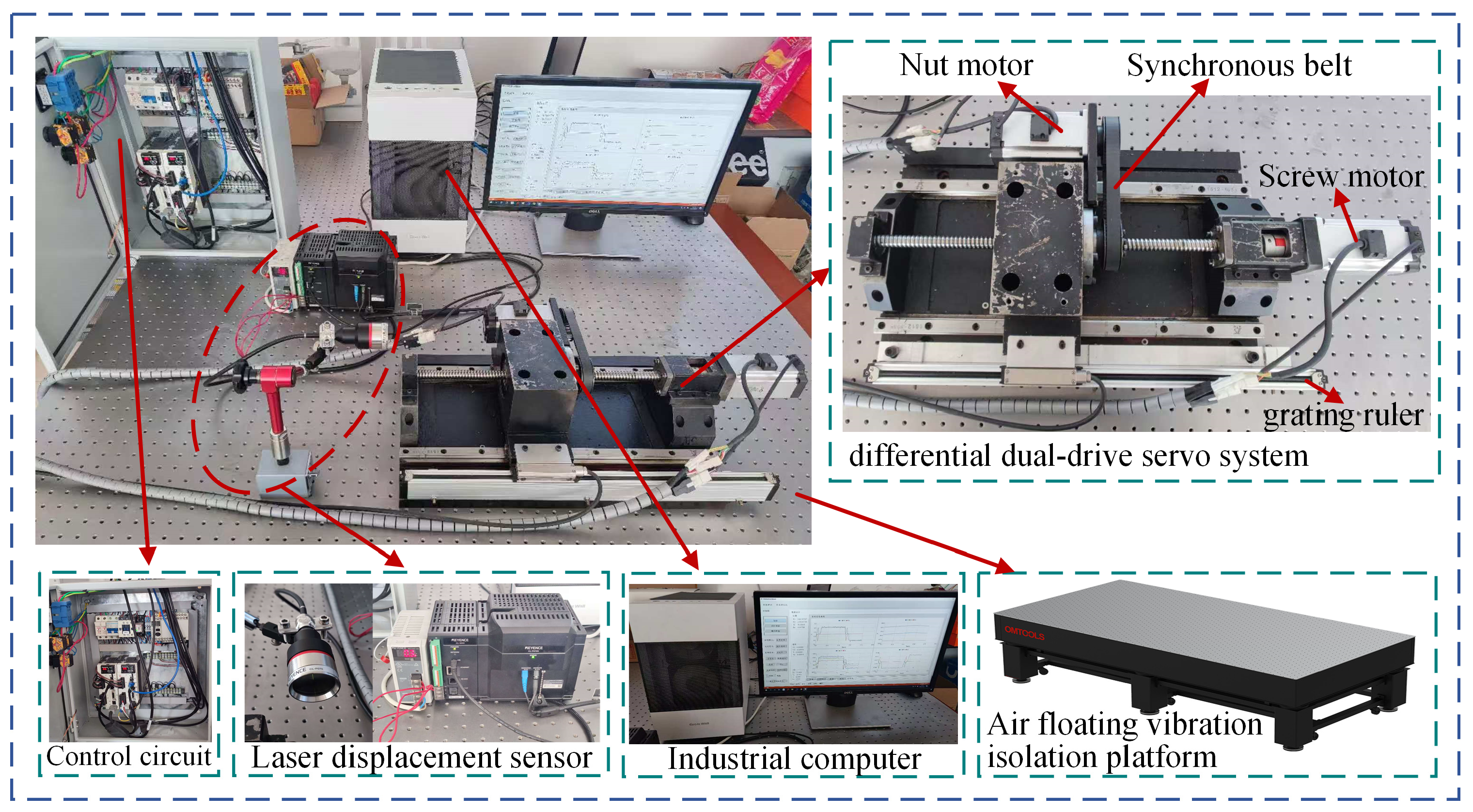
In order to verify the effectiveness of the proposed control scheme, the experimental verification is carried out in the differential dual-drive servo system. The hardware structure is shown in Figure 5. It includes an industrial computer, control circuit, differential dual-drive servo system, EtherCAT communication driver, laser displacement sensor and air floating vibration isolation platform. The differential dual-drive servo system includes a screw–nut pair, a screw motor that drives the screw rotation, a nut motor that drives the nut rotation, a synchronous belt, a grating ruler, a LM guide rail, and a workbench. The screw motor and the nut motor are equipped with an absolute rotary encoder. The model of the roller screw–nut pair is DIR1605-THK, and the model of the precision grating ruler is GVS600T001E, with a resolution of 10 nm.
The feedforward controller based on iterative learning requires the initial state of each experiment to be the same. The laser displacement sensor of model CL-3000 is fixed on the air bearing platform to detect the absolute position of the worktable. The absolute position of the two motors is detected by an absolute rotary encoder so as to ensure that the initial state of the workbench and the two motors are consistent in each iteration experiment. The whole experimental system is arranged on the air floating vibration isolation platform, which can reduce the influence of environmental disturbance on the experimental measurement results.
In the experiments, periodic disturbances mainly arose from repetitive errors inherent to the system, rather than from additional injection by external devices. Specifically, the periodic disturbances included cogging torque, flux-linkage harmonics, installation errors, and repetitive friction. The worktable position, motor angle, and motion speed showed strong repeatability across different iterations. Therefore, these disturbances reappeared in a manner related to the absolute position. In addition, non-periodic disturbances included parameter uncertainty, unmodeled dynamics, non-repetitive friction caused by state changes, and external sudden disturbances. In the experiments, sudden disturbances were introduced by applying an equivalent load torque. A step disturbance with an equivalent control input was applied to the motor torque channel to simulate an external sudden load or disturbance. The disturbance rejection performance was evaluated by the speed fluctuation and the position tracking error. The rotational inertia was taken as the equivalent rotational inertia of the system. This parameter was identified by frequency-sweep experiments and the least-squares method [24]. The worktable position was measured by a high-precision linear encoder and was used to calculate the worktable tracking error and evaluate the final positioning accuracy. The angular positions of the screw motor and the nut motor were measured by their respective absolute rotary encoders to obtain the motor-side position and speed information. A laser displacement sensor was used to detect the absolute position of the worktable, mainly to ensure a consistent initial position before each iterative experiment. The speed signal was obtained by differentiating the position measurement signal. To reduce the high-frequency noise introduced by differentiation, the speed signal was processed by a digital low-pass filter before being used for feedback control, speed fluctuation analysis, and frequency-domain analysis. All experimental data, including the worktable position, motor position, speed signal, tracking error, and control input, were synchronously collected at a sampling frequency consistent with that of the control signal.
For the designed parametric feedforward controller, the basis function is selected: φ 1 = z 1 z T s , φ 2 = φ 5 = ( z 1 z T s ) 2 , φ 3 = φ 6 = ( z 1 z T s ) 3 , φ 4 = φ 7 = ( z 1 z T s ) 4 . T s is the sampling period. The discrete transfer function of the controlled object can be expressed as P ( z ) = 0.0002147 z + 0.0002086 z 2 1.917 z + 0.9174 , and the feedback controller adopts PD control, C f b ( z ) = 0.026 z 2 0.00086 z + 0.00087 z 2 1.96 z . The parameter vector to be identified is θ = [ 0 , 0 , 0 , 0 , 0 , 0 , 0 ] T . In addition, ρ 1 = 5 × 10 9 and ρ 2 = 2 × 10 8 .
For the designed sliding mode controller based on the super-twisting sliding mode observer, the control parameters are continuously adjusted by means of engineering tuning. Finally, the parameters are selected as follows: k = 0.06 , p = 30 , c = 0.003 , ε = 0.1 , δ = 0.8 , c o b = 5 , α = 80 , λ = 1000 . The parameters of the resonant controller are as follows: κ 1 = 5 , φ r 1 = π 18 , κ 2 = 8 , φ r 2 = π 9 .
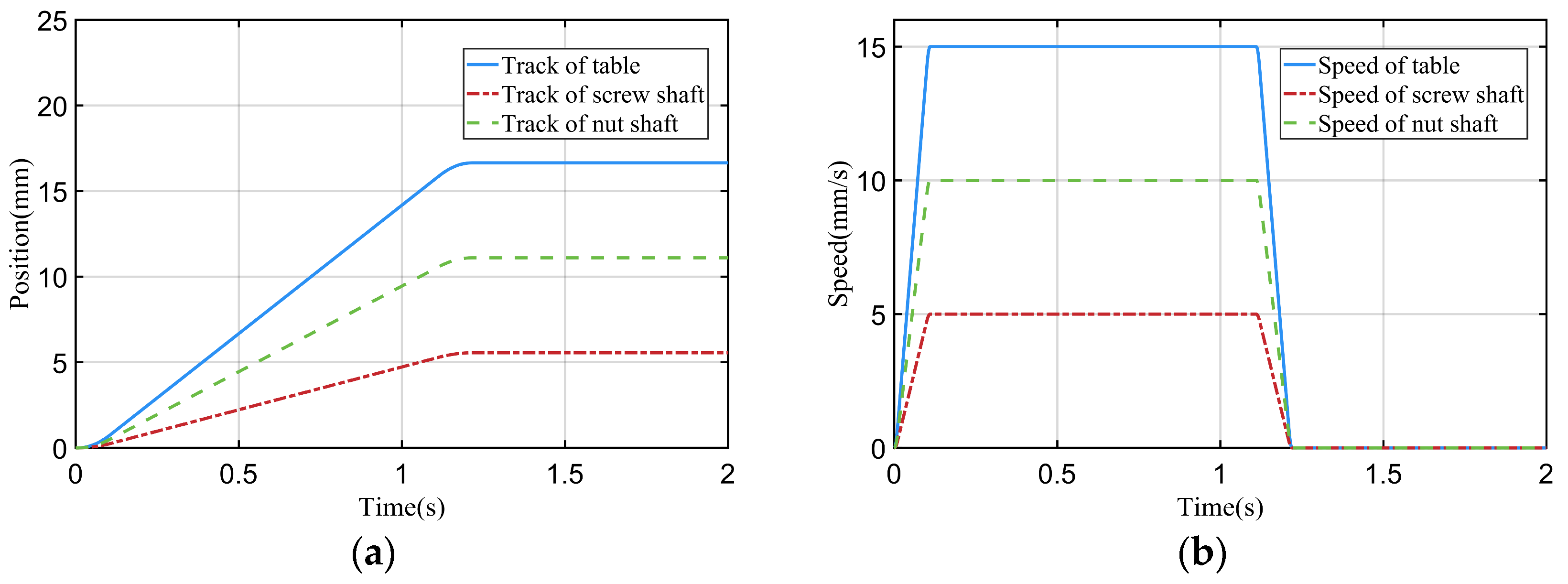
The experimental reference trajectory is a fourth-order S-shaped curve, as shown in Figure 6. Displacement, velocity and acceleration are smooth and continuous signals, which are suitable for high-speed and high-precision tracking control. According to the movement, it is divided into an acceleration stage, a uniform speed stage, a deceleration stage and a zero-speed stage. The sampling frequency is the same as the control signal transmission frequency, which is 4000 Hz. During the experiment, the rotating motion signal of the motor is equivalent to the linear motion signal of the screw shaft and the nut shaft. The transmission ratio of linear motion and rotary motion is r = P h / ( 2 π η ) . Among them, P h is the screw lead and η is the transmission efficiency of the servo system. The parameters of the differential dual-drive servo system are shown in Table 2, and the model parameters of the screw motor and the nut motor are exactly the same.

5.2. Experimental Results and Discussion

Experiments are carried out in the differential dual-drive servo system shown in Figure 5. The nut motor adopts the sliding mode controller based on the super-twisting sliding mode observer proposed in this study for feedback control. The screw motor adopts the feedforward controller based on iterative learning proposed in this study, which is combined with the PD controller to realize the two-degree-of-freedom control combining feedback control and feedforward control. The disturbance of various mechanical transmission components such as the screw motor, the nut motor and the workbench will be reflected in the tracking error of the workbench. The nut motor realizes the suppression of non-periodic disturbances and time-varying disturbances through the error of the current control cycle feedback and can cope with events such as sudden load changes. Through continuous iterative learning of the error of the previous iterative process, the screw motor can reduce tracking error and improve tracking accuracy.
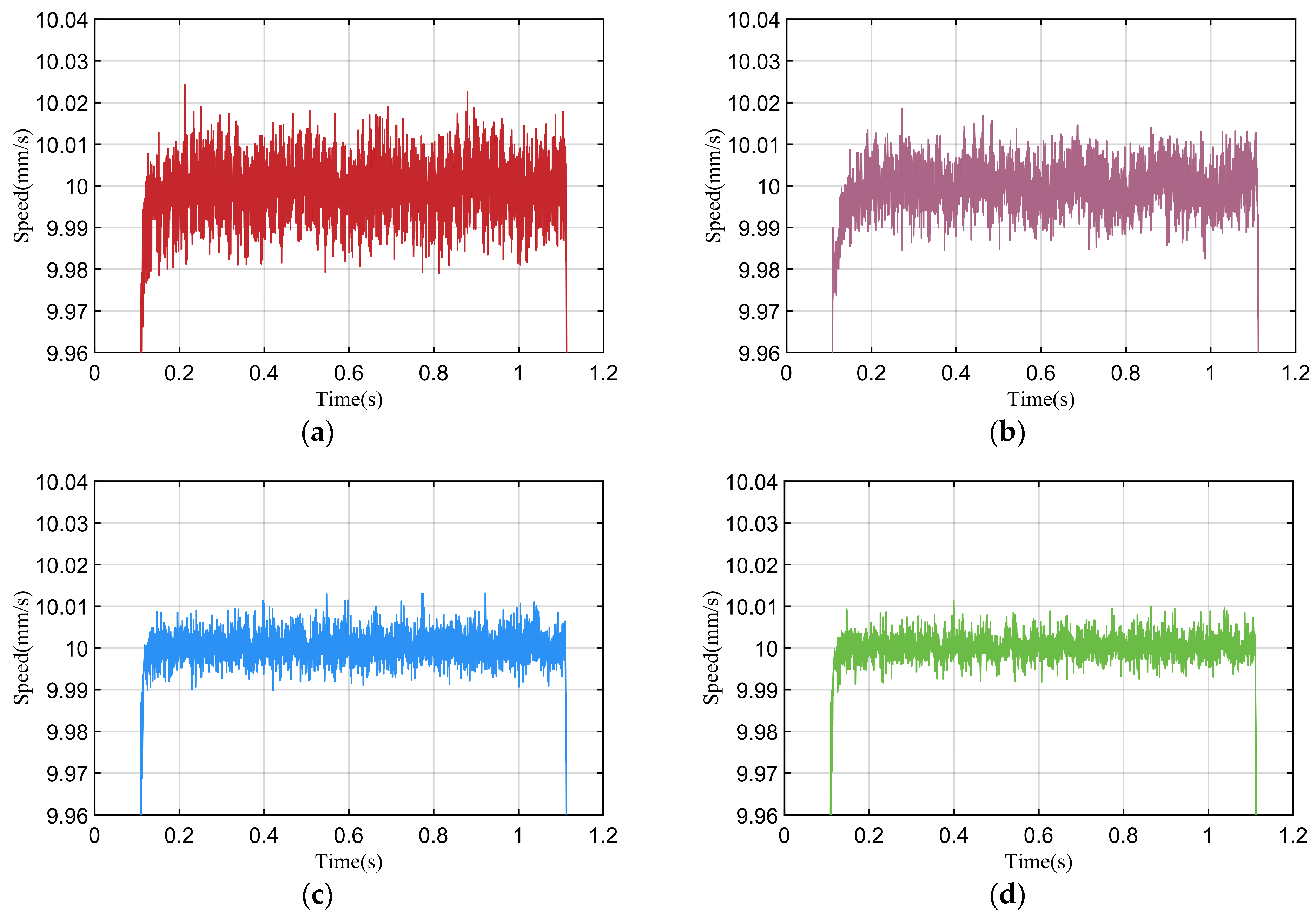
Figure 7 shows the speed tracking of the workbench under different iterations. The figure mainly shows the speed response of the workbench in the uniform speed stage. Figure 7a shows the speed tracking results of the first iteration, and the speed fluctuates from 9.979 mm/s to 10.024 mm/s. The velocity has large oscillations and obvious low-frequency sinusoidal fluctuation. Figure 7b is the result of the velocity tracking experiment of the fifth iteration, and the velocity fluctuates from 9.983 mm/s to 10.018 mm/s. The velocity fluctuation is slightly improved compared to the first iteration result, but there is still a significant low-frequency sinusoidal fluctuation with the same frequency as the first iteration. This is because the differential dual-drive servo system is composed of a screw motor, nut motor, workbench, synchronous belt and guide rail. In the process of repeated movement, the elastic deformation of the synchronous belt will cause periodic torque fluctuation. In addition, manufacturing errors such as clearance and pitch errors of transmission parts such as roller screw–nut pairs and installation errors such as couplings and bearings will cause periodic disturbances to a certain extent, further causing periodic errors of the workbench. These errors are generally manifested as low-frequency components. Figure 7c is the result of the velocity tracking experiment of the 10th iteration, and the velocity fluctuation is obviously reduced. The speed is stable in the range of 9.991 mm/s to 10.014 mm/s. Figure 7d is the experimental result of the 15th iteration, and the speed is stable in the range of 9.998 mm/s to 10.012 mm/s. The speed tracking performance is significantly improved compared with the first iteration, and it is also improved to a certain extent compared with the 10th iteration. From the 10th iteration, the experimental results begin to converge, and the 15th iteration is completely convergent. The experimental results of the subsequent iterations are very different. After the 10th iteration, the low-frequency sinusoidal fluctuation is obviously suppressed. At the beginning of each iteration, the laser displacement sensor, encoder and other sensors are used to ensure that the initial state of the motor and the workbench is consistent. This means that the periodic disturbances caused by installation error, manufacturing error and transmission error are the same in each iteration. Through the iterative learning of the workbench error, the parameters of the feedforward controller are continuously optimized to achieve a strong suppression of periodic disturbances.
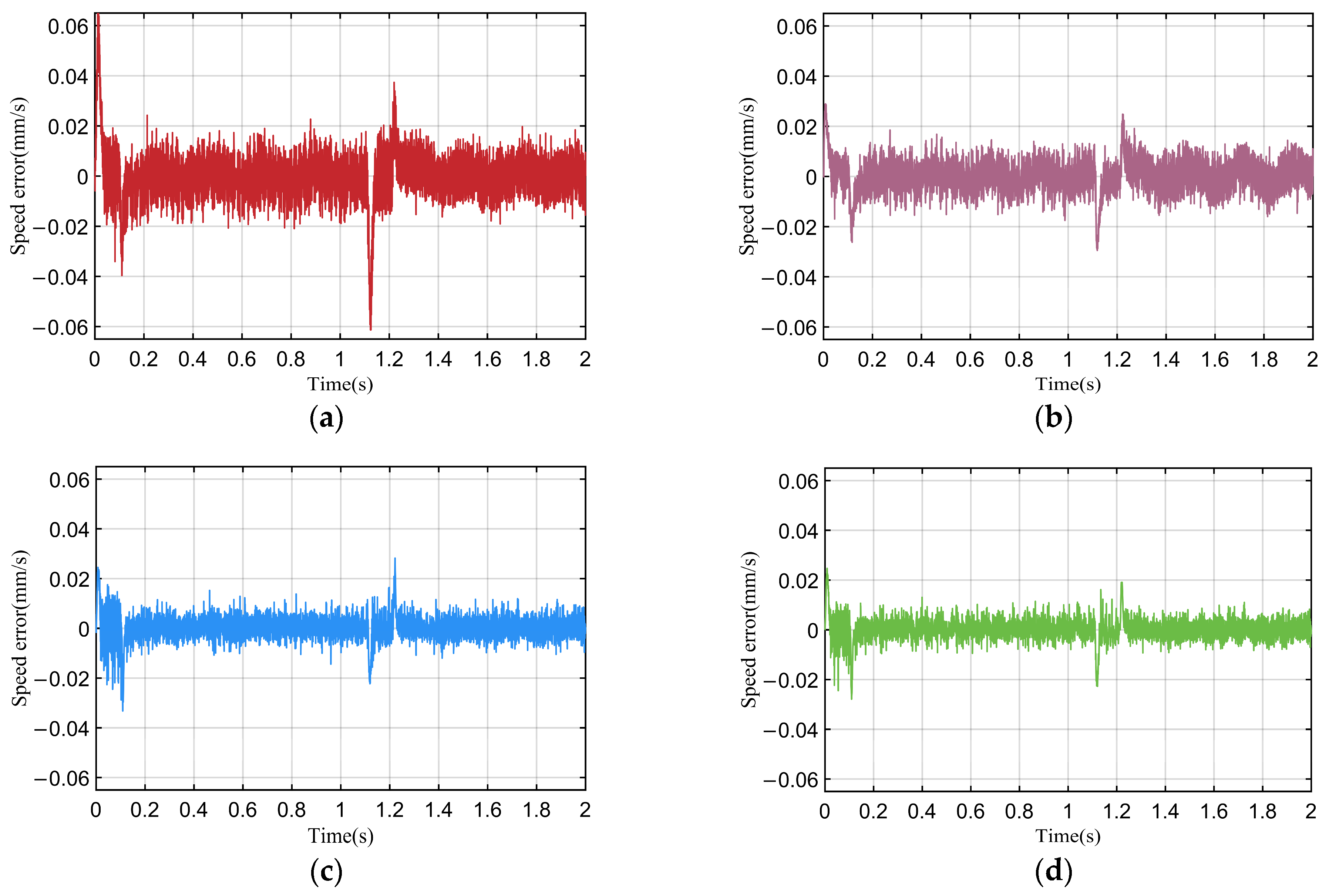
The speed tracking error curve is shown in Figure 8. The figure shows the speed tracking errors of the acceleration, uniform speed, deceleration and zero-speed stages of the fourth-order S-shaped trajectory tracking curve. Figure 8a is the velocity error of the first iteration. In the acceleration phase and the deceleration phase, the acceleration increases first, and the error then accumulates rapidly. When the acceleration is constant, the error decreases and fluctuates around the zero value. Then the acceleration is reduced to complete the acceleration and deceleration processes. Due to the change in acceleration, the error increases again. Compared with the uniform speed and zero-speed stage, the error is larger, reaching 0.063 mm/s. In the uniform speed and zero-speed stage, the speed error is stable within ±0.022 mm/s. Figure 8b shows the velocity error of the fifth iteration. The error in the acceleration and deceleration stages is significantly reduced, and the maximum value is only 0.028 mm/s. The uniform speed and zero-speed stages also have a certain degree of improvement, and the error fluctuates within ±0.019 mm/s. Figure 8c is the velocity error of the 10th iteration. At this time, the iteration has begun to converge gradually, and the velocity tracking error is further reduced. Figure 8d is the speed error of the 15th iteration, and the iteration is completely convergent. The maximum error in the acceleration and deceleration phases is only 0.023 mm/s. The tracking accuracy is improved by 63.49% compared with the first iteration. The velocity error in the uniform speed and zero-speed stages is stable at ±0.012 mm/s, which is 45.45% lower than in the first iteration.
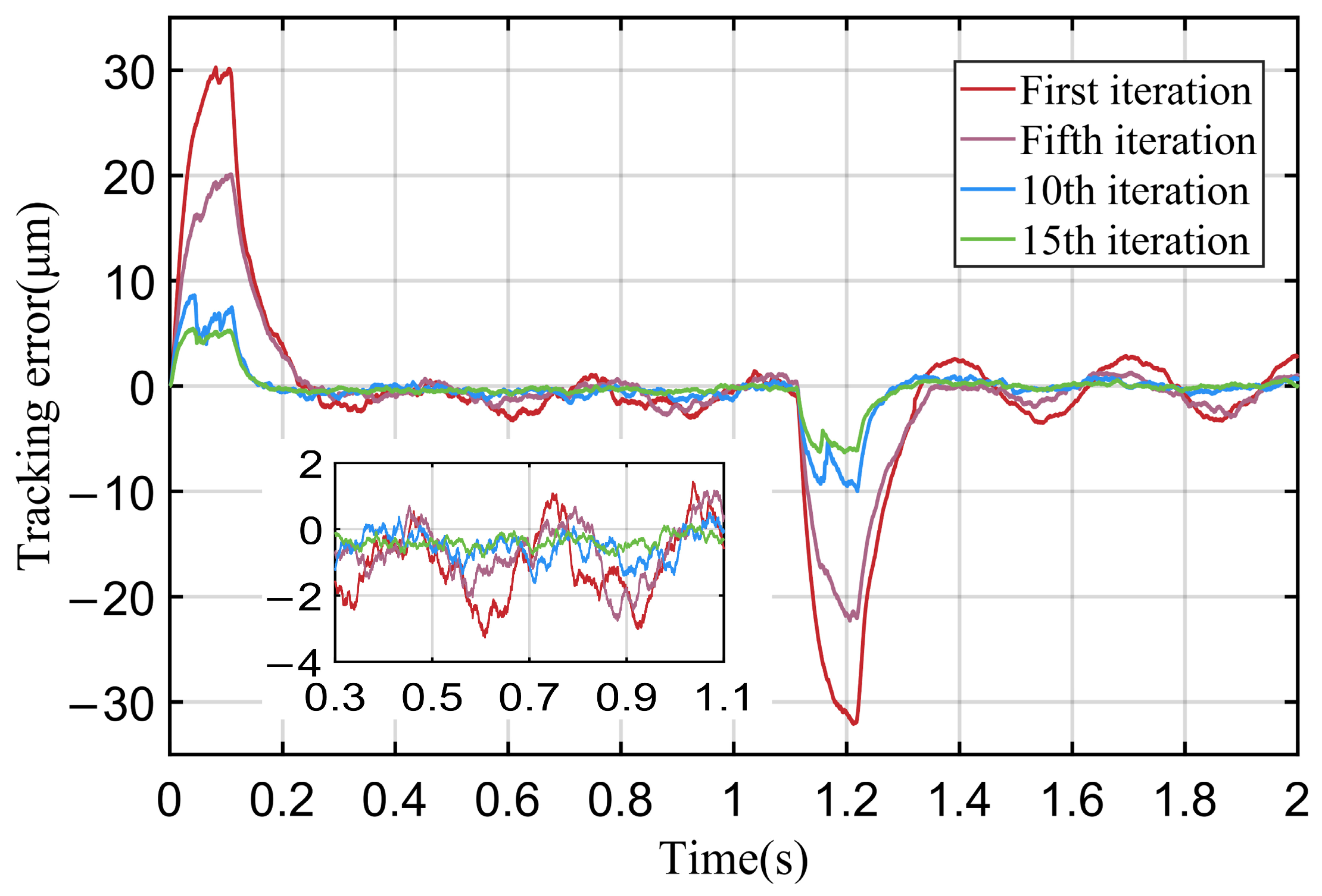
The displacement tracking error is further analyzed. Figure 9 shows the displacement tracking error of the workbench in different iterative processes. In the first iteration, the tracking error gradually increases in the acceleration phase and gradually decreases after reaching 30 μm. In the uniform phase, the tracking error is stable in the range of −4 μm to 2 μm. In the deceleration phase, the tracking error again accumulates to −32 μm. In the zero-speed stage, the error is stable in the range of ±4 μm. As the number of iterations increases, the tracking error gradually decreases. In the fifth iteration, the tracking error reaches a maximum of 22 μm in the deceleration phase. In the 10th iteration, the tracking error in the acceleration phase reaches a maximum of 9 μm, the tracking error in the deceleration phase reaches a maximum of 10 μm, and the tracking error in the uniform phase is stable in the range of −1.8 μm to 0.8 μm. The tracking error is significantly improved in the 15th iteration. In the acceleration stage, the error tends to be stable after reaching 5 μm. When entering the uniform stage, the error decreases rapidly and stabilizes in the range of −1 μm to 0.2 μm. The error accumulates to −6.5 μm again during deceleration. When the speed is zero, the error approaches zero and fluctuates in a very small range, and the positioning accuracy is continuously adjusted. Compared with the first iteration, the tracking accuracy is significantly improved. The tracking error in the acceleration stage is reduced by 83.3%, the tracking error in the uniform speed stage is reduced by 75%, and the error in the deceleration stage is reduced by 79.7%. In addition, in the first iteration, the error tends to be stable at 0.25 s when transitioning from the acceleration phase to the uniform phase. In the 15th iteration, the error tends to be stable at 0.18 s, and the time for the error to reach the stable stage is significantly reduced. In summary, with the increase in the number of iterations, the proposed control scheme can significantly suppress the disturbance and improve the tracking accuracy of the system.
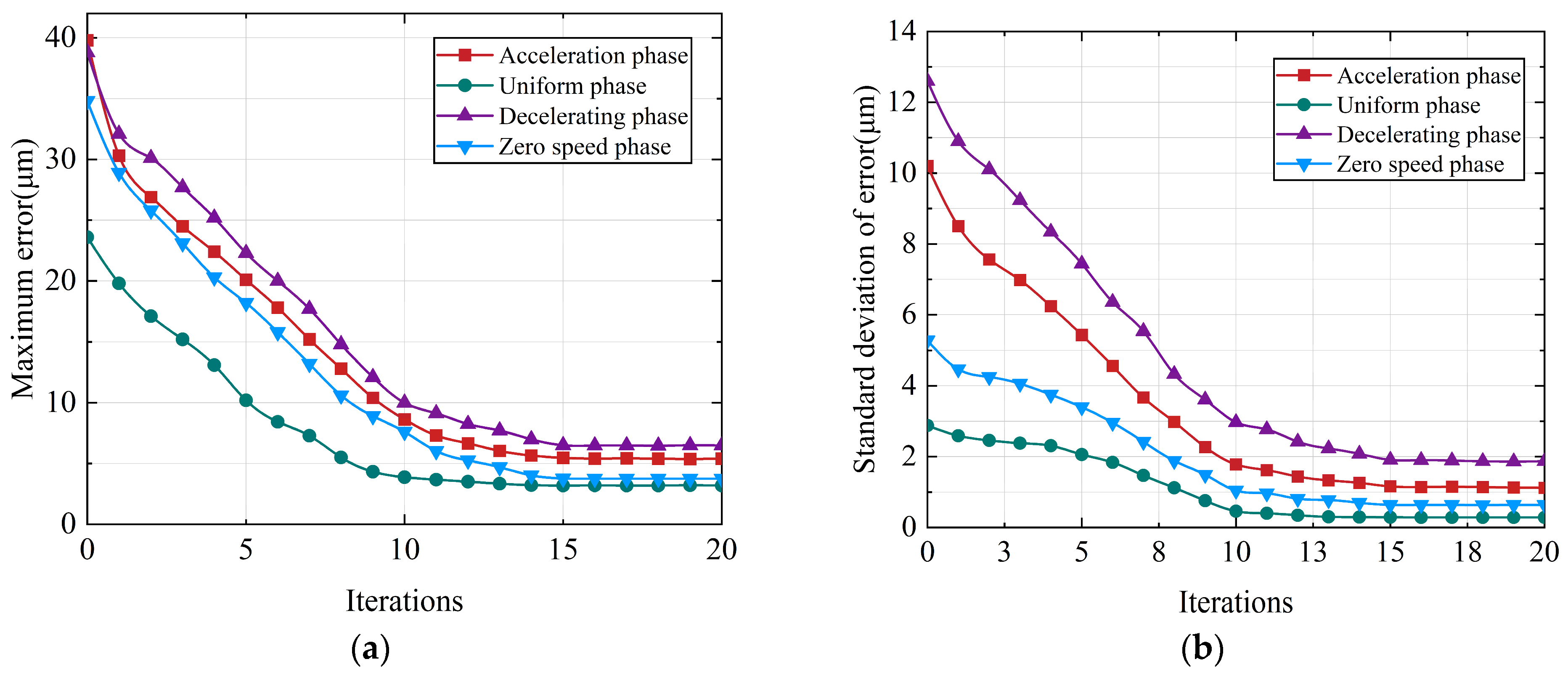
Figure 10 shows the convergence of error iteration in each motion stage. Figure 10a is the maximum value of the tracking error, and Figure 10b is the standard deviation of the tracking error. In the whole movement process, 0–0.12 s is the acceleration movement stage, 0.12–1.1 s is the uniform movement stage, 1.1–1.22 s is the deceleration movement stage, and 1.22–2 s is the zero-speed movement stage. It can be seen from Figure 10a that the maximum tracking error of the four motion stages gradually decreases with the increase in the number of iterations, and it is significantly reduced and begins to converge at the 10th iteration. After the 15th iteration, the error is completely convergent. Figure 10b shows the convergence of the standard deviation in each stage. In the initial iteration, the standard deviation is large. This means that the tracking error of each stage has a wide range of fluctuation, a large degree of dispersion, and a relatively scattered data distribution. As the number of iterations increases, the standard deviation of each stage gradually decreases and converges. After the 15th iteration, the standard deviation of the error in the deceleration stage is 1.91 μm, the standard deviation of the error in the acceleration stage is 1.16 μm, the standard deviation of the error in the uniform speed stage is 0.288 μm, and the standard deviation of the error in the zero-speed stage is 0.639 μm. Compared with the first iteration, the error fluctuation of each stage is significantly reduced, and the error data distribution is more concentrated. In the whole iteration process, the maximum error and standard deviation in the acceleration and deceleration stages are greater than those in the uniform speed and zero-speed stages due to the change in nonlinear disturbance such as nonlinear friction caused by the change in speed.
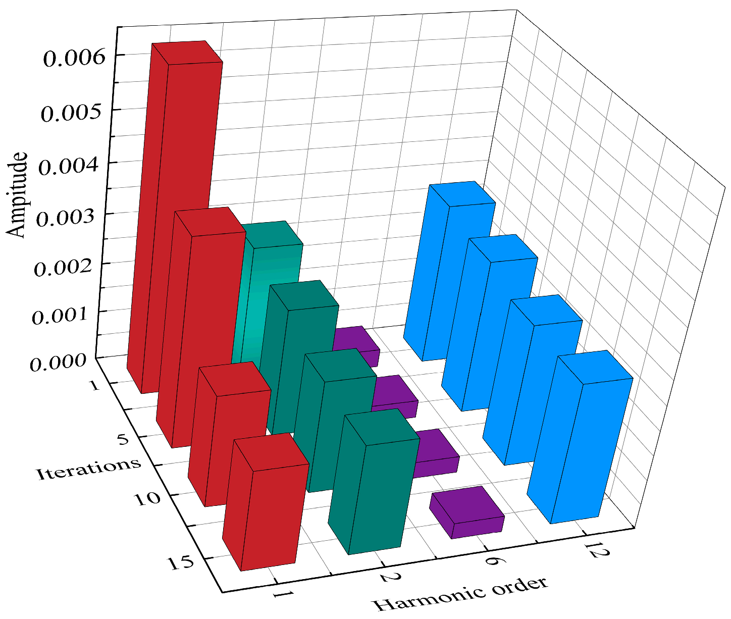
Figure 11 shows the velocity harmonic amplitude in the uniform speed stage. The data collected when the speed reaches a stable state are selected for Fourier transform, and the changes in the 1st harmonic, 2nd harmonic, 6th harmonic and 12th harmonic throughout the iterative process are counted. It can be seen from the figure that the amplitude of the first harmonic decreases significantly with the increase in the number of iterations, and the amplitude of the second harmonic decreases to a certain extent in the 15th iteration. However, the degree of reduction is relatively lower than that of the first harmonic. The 6th harmonic and 12th harmonic are not obvious in the iterative process. It can be seen that the control scheme proposed in this paper can reduce the amplitude of the first harmonic and the second harmonic. This means that the iterative process reduces the amplitude of the low-frequency band to varying degrees. However, the iterative process has no significant effect on reducing the amplitude of the 6th and 12th harmonics.
Relevant literature [22] has proven that the differential dual-drive motion mode has better low-speed performance than the traditional conventional single-drive mode, which can significantly improve the motion accuracy. Therefore, this paper conducts comparative experiments in the differential dual-drive motion mode to verify the effectiveness of the control scheme proposed in this paper. The reference trajectory shown in Figure 6 is adopted, and the comparative experiments are carried out according to the experimental scheme in Table 3. In method 1–method 5, the workbench is driven by a screw motor and a nut motor at the same time. And in method 1–method 4, the screw motor and the nut motor adopt the same control algorithm. Method 1 is an adaptive friction compensation controller (AFCC) [25]. Method 2 is a PD controller based on friction feedforward compensation (PD-FFFC) [24]. Method 3 is a sliding mode controller based on a generalized extended state observer (GESO-SMC). Method 4 is a sliding mode controller based on the super-twisting sliding mode observer (STSMO-SMC) proposed in this paper. In method 5, the screw motor and the nut motor adopt different control methods. The nut motor adopts STSMO-SMC, and the screw motor adopts the feedforward controller based on iterative learning (ILFFC) proposed in this paper.
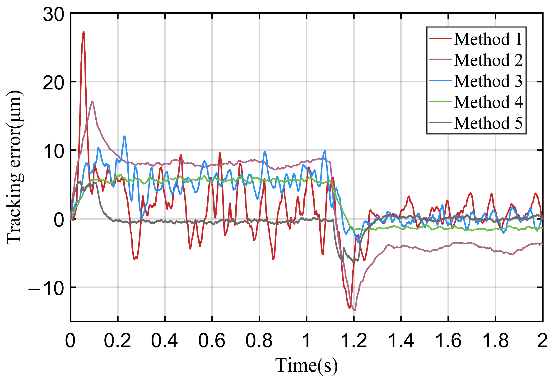
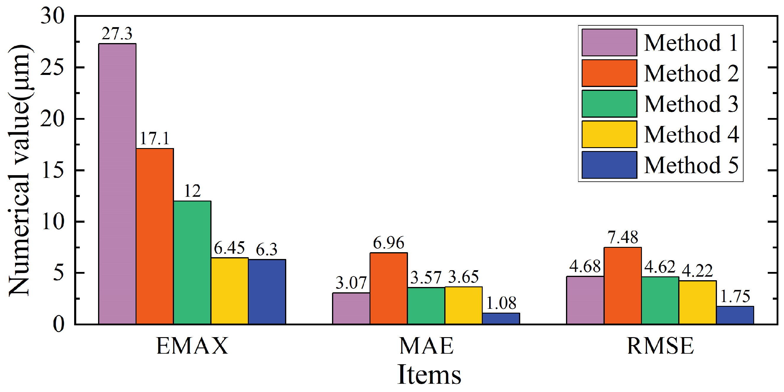
Figure 12 shows the experimental results of the workbench tracking error under various control methods. Figure 13 shows the statistical result of the tracking error of the workbench. The evaluation indicators are the maximum absolute error (EMAX), the mean absolute error (MAE), and the root mean square error (RMSE) so that the methods can be assessed comprehensively in terms of peak deviation, overall average error, and error fluctuation. The maximum tracking error of method 1 is 27.3 μm, which appears in the acceleration phase. In the uniform stage, the error is stable within −6 μm to 9 μm. The error of the zero-speed stage is stable within 4 μm. In the process of adaptive adjustment, the control parameters change greatly, resulting in a large fluctuation of tracking error. Method 2 introduces friction feedforward compensation on the basis of PI control. In the uniform speed stage, the friction force almost does not change, and the friction compensation effect is more obvious. Compared with the acceleration and deceleration phases, the tracking error is significantly reduced and stabilized at about 8 μm. The error in the zero-speed stage is stable at about −4 μm. The generalized extended state observer of method 3 can estimate and compensate for the external disturbance. The error of the uniform movement stage fluctuates in the range of 0–12 μm. The error in the zero-speed stage is stable within ±3 μm. Method 4 has small error fluctuation due to the accurate observation of the disturbances by the super-twisting sliding mode observer. The RMSE is 4.22 μm, and the uniform speed stage fluctuates in a small range around 5 μm. At the zero-speed stage, the error is about −2 μm. According to the above analysis, through the comparison of methods 1 to 4, it is found that the sliding mode controller based on the super-twisting sliding mode observer proposed in this paper has stable performance, a significant improvement in accuracy, and a more excellent control effect. The control effect of Method 5 is significantly improved. The error reaches a maximum of 6.3 μm in the acceleration and deceleration phases. The error in the uniform stage fluctuates in the range of −1 μm to 0.2 μm. The error of the zero-speed stage is stable at ±0.5 μm. And compared with other methods, the proposed method has the smallest RMSE and MAE. The results indicate that the proposed method exhibits superior suppression performance for periodic disturbances under repetitive trajectories. This is because the introduction of iterative learning feedforward control suppresses the residual errors that feedback control is unable to compensate for. This significantly improves the control accuracy of the proposed method.
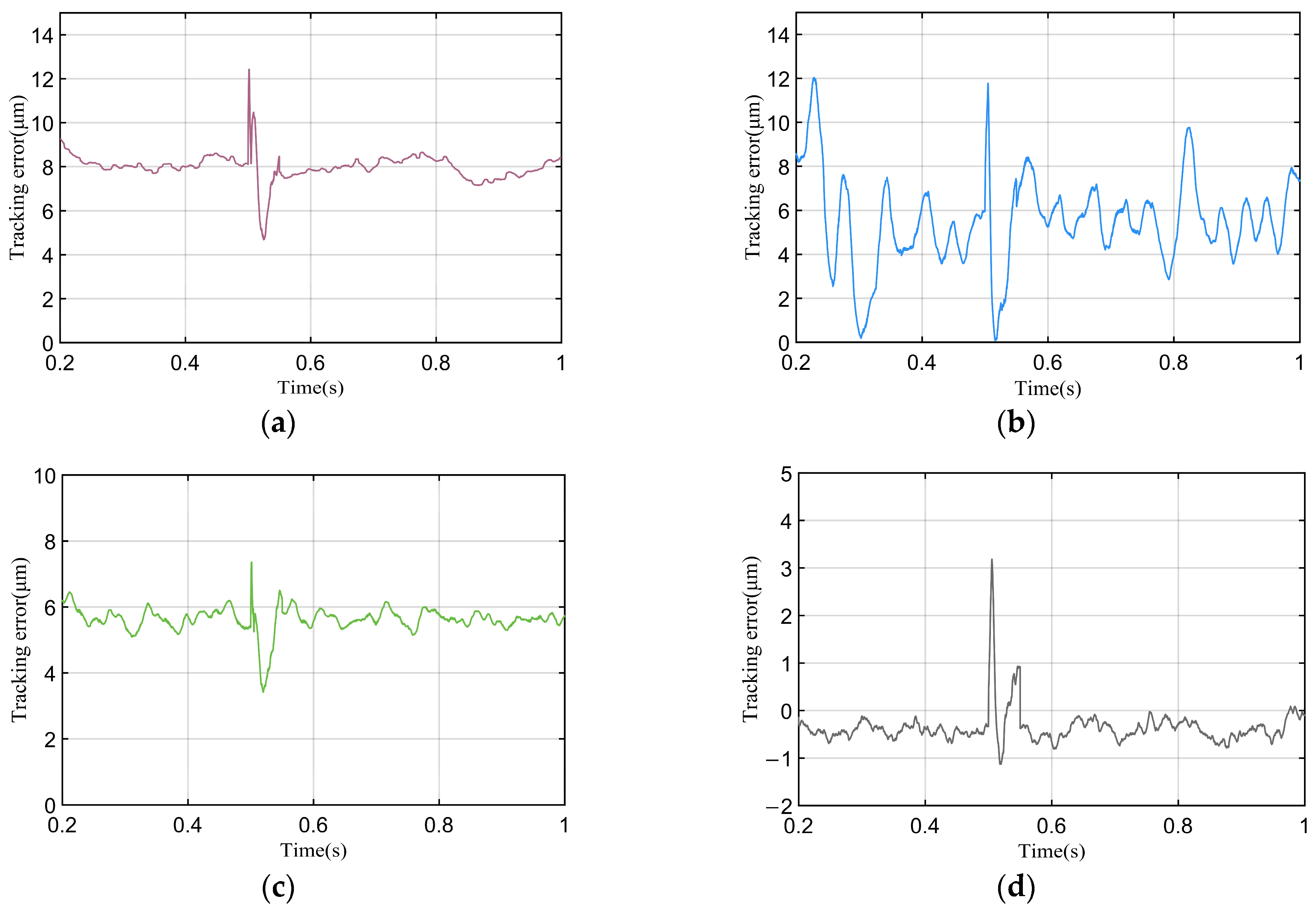
In order to verify the resistance of the proposed control scheme to the sudden disturbance, a sudden disturbance of 0.15 Nm is applied at 0.5 s. The adaptive friction compensation controller does not have good resistance to abrupt interference, so the other four methods are compared. The displacement tracking error curve of the workbench in the uniform speed stage is shown in Figure 14. Statistical results of mutation perturbation inhibition are shown in Table 4. The four methods have certain resistance to the disturbance mutation and can quickly adjust and stabilize the error. Figure 14a shows the error curve of method 2 when an abrupt perturbation is applied. After the disturbance is applied, the error increases rapidly, and the change value reaches 7.8 μm. From Figure 14b, it can be seen that the error change value of method 3 is 12 μm after the disturbance is applied. Figure 14c is the error curve of method 4 when abrupt perturbation is applied. The error change value reaches 3.9 μm, and the recovery time is 0.045 s. Figure 14d is the error curve of method 5 when an abrupt disturbance is applied. The maximum error change reaches 4.2 μm, and the recovery time is 0.048 s. The maximum error change and recovery time of method 4 and method 5 are less than those of method 2 and method 3 when an abrupt disturbance is applied. This proves that the STSMO-SMC proposed in this paper has a better suppression effect on sudden disturbance. For method 5, when a sudden disturbance occurs, its influence is mapped to the tracking accuracy of the workbench. The nut motor observes the disturbance using the super-twisting sliding mode observer based on the current feedback error signal. The disturbance is compensated in real time by the nut motor. The screw motor updates the feedforward controller parameters according to the error of the previous iteration cycle to achieve precise feedforward control. And the RMSE of Method 5 when it reaches stability after the disturbance is applied is also the lowest among the other methods. This means that the STSMO-based feedback loop mainly contributes to the fast rejection of sudden non-periodic disturbances, while the ILFFC component further improves steady-state tracking accuracy.

6. Conclusions

In order to reduce the influence of periodic disturbances and non-periodic disturbances on the tracking performance of the servo system, a dual-motor drive compound control strategy based on an iterative learning feedforward controller and super-twisting sliding mode observer is proposed in this paper. Firstly, a sliding mode controller based on a super-twisting sliding mode observer is proposed to suppress the influence of non-periodic disturbances, and a new reaching law, which can dynamically adjust the variable gain coefficient according to the system state and improve the control performance of the system, is designed. The resonant controller is designed and connected in parallel with the SMC to suppress the influence of medium- and high-frequency disturbances. Secondly, in order to reduce the influence of periodic disturbances on the control accuracy of the system, a parametric feedforward controller based on iterative learning is proposed on the basis of the two-degree-of-freedom control structure and the input-shaping filter. The parameters are iteratively updated in a data-driven manner. By learning the error of the previous iteration period, the periodic disturbances in the current iteration process are effectively suppressed. A differential dual-drive servo system model is established. The motion of the workbench is composed of two motors that drive the screw and nut rotation. The nut motor adopts STSMO-SMC, and the screw motor adopts ILFFC. The periodic and non-periodic disturbances of the workbench can be effectively suppressed by the two motors. This solves the problem that the parametric feedforward controller based on iterative learning and the high robustness controller are difficult to combine. Experiments show that the STSMO-based feedback loop mainly contributes to fast rejection of sudden non-periodic disturbances, while the ILFFC component further improves steady-state tracking accuracy. Therefore, this method not only improves the tracking accuracy of the system but also takes into account the robust performance of the system.

Author Contributions

Conceptualization, A.W. and X.F.; methodology, A.W.; software, A.W.; validation, A.W., H.W. and X.F.; formal analysis, M.Y.; investigation, M.Y.; resources, X.F.; data curation, A.W. and H.W.; writing—original draft preparation, A.W.; writing—review and editing, A.W.; visualization, X.F.; supervision, X.F.; project administration, A.W.; funding acquisition, X.F. All authors have read and agreed to the published version of the manuscript.

Funding

This research was funded by the National Natural Science Foundation of China, grant number 51875325; and the Key Research and Development Plan of Shandong Province, grant number 2022CXGC010101.

Institutional Review Board Statement

Not applicable.

Informed Consent Statement

Not applicable.

Data Availability Statement

The datasets generated or analyzed during this study are available from the corresponding author on reasonable request.

Acknowledgments

The authors would like to thank the Key Laboratory of High Efficiency and Clean Mechanical Manufacture of the Ministry of Education for their support of the research and experiments.

Conflicts of Interest

The authors declare no conflicts of interest.

Abbreviations

The following abbreviations are used in this manuscript:
SMCSliding mode control
ILCIterative Learning Control
PMSMPermanent magnet synchronous motor
AFCCAdaptive friction compensation controller
GESO-SMCSliding mode controller based on generalized extended state observer
STSMO-SMCSliding mode controller based on super-twisting sliding mode observer
ILFFCFeedforward controller based on iterative learning

References

  1. Qian, L.; Sun, L.; Wang, K.; Tong, M. Fusion of Position Estimation Techniques for a Swing Servo by a Permanent-Magnet Synchronous Machine. IEEE Trans. Ind. Electron. 2023, 70, 6551–6562. [Google Scholar] [CrossRef] [Scilit]
  2. Sun, L.; Li, X.; Chen, L.; Shi, H.; Jiang, Z. Dual-Motor Coordination for High-Quality Servo With Transmission Backlash. IEEE Trans. Ind. Electron. 2023, 70, 1182–1196. [Google Scholar] [CrossRef] [Scilit]
  3. Wang, T.; Zhang, Q.; Fang, J.; Lai, Z.; Feng, R.; Wei, J. Active fault-tolerant control for the dual-valve hydraulic system with unknown dead-zone. ISA Trans. 2023, 145, 399–411. [Google Scholar] [CrossRef] [Scilit] [PubMed]
  4. Yao, X.; Zhang, L.; Cui, Y. Adaptive Refined Disturbance Observer-Based Velocity-Tracking Control for Gimbal Servo System With Multiple Disturbances. IEEE Trans. Syst. Man Cybern. Syst. 2024, 54, 7170–7181. [Google Scholar] [CrossRef] [Scilit]
  5. Cui, Y.; Zhu, Y.; Liu, J.; Wang, C.; Zhao, L. Analysis, Estimation, and Rejection of Multi-Frequency Unknown Disturbances in CMG Gimbal Servo Systems. IEEE Trans. Circuits Syst. II-Express Briefs 2024, 71, 4501–4505. [Google Scholar] [CrossRef] [Scilit]
  6. Tang, C.; Fan, Y.; Yang, C.; Cheng, M.; Lee, C.H.T. Friction Identification and Compensation for SPMSM Using Robust Adaptive Observer. IEEE J. Emerg. Sel. Top. Power Electron. 2024, 12, 4754–4766. [Google Scholar] [CrossRef] [Scilit]
  7. Niu, S.; Wang, J.; Zhao, J.; Shen, W. Neural network-based finite-time command-filtered adaptive backstepping control of electro-hydraulic servo system with a three-stage valve. ISA Trans. 2024, 144, 419–435. [Google Scholar] [CrossRef] [Scilit] [PubMed]
  8. Li, J.; Li, Y.; Li, X.; Mao, D.; Zhang, B. Adaptive Disturbance Suppression Method for Servo Systems Based on State Equalizer. Sensors 2024, 24, 4418. [Google Scholar] [CrossRef] [Scilit] [PubMed]
  9. Junejo, A.K.; Xu, W.; Mu, C.; Ismail, M.M.; Liu, Y. Adaptive Speed Control of PMSM Drive System Based a New Sliding-Mode Reaching Law. IEEE Trans. Power Electron. 2020, 35, 12110–12121. [Google Scholar] [CrossRef] [Scilit]
  10. Hou, Q.; Ding, S.; Yu, X. Composite Super-Twisting Sliding Mode Control Design for PMSM Speed Regulation Problem Based on a Novel Disturbance Observer. IEEE Trans. Energy Convers. 2021, 36, 2591–2599. [Google Scholar] [CrossRef] [Scilit]
  11. Shi, S.; Dai, L.; Min, H.; Yang, J.; Li, S. Prescribed-Time Nonsingular Terminal Sliding Mode Control and Its Application in PMSM Servo Systems. IEEE Trans. Ind. Electron. 2024, 72, 3072–3081. [Google Scholar] [CrossRef] [Scilit]
  12. Zhufu, G.; Wang, S.; Wang, X. Finite time disturbance observer based sliding mode control for PMSM with unknown disturbances. Int. J. Robust Nonlinear Control 2024, 34, 7547–7564. [Google Scholar] [CrossRef] [Scilit]
  13. Gao, Y.; Shen, G.; Li, X.; Zhu, Z.; Wang, Q. An Improved Nonlinear Extended Disturbance Observer for Sliding Mode Control in Electro-Hydraulic Servo System. IEEE/ASME Trans. Mechatron. 2024, 30, 2155–2164. [Google Scholar] [CrossRef] [Scilit]
  14. Sun, Y.; Yang, M.; Wang, B.; Chen, Y.; Xu, D. Precise Position Control Based on Resonant Controller and Second-Order Sliding Mode Observer for PMSM-Driven Feed Servo System. IEEE Trans. Transp. Electrif. 2023, 9, 196–209. [Google Scholar] [CrossRef] [Scilit]
  15. Zhang, C.; Qi, R.; Li, B.; Riaz, S. Experimental validation and analysis of hybrid adaptive iterative learning sliding mode control for PMSM seeker coordinator. Eng. Sci. Technol. Int. J. 2024, 58, 101826. [Google Scholar] [CrossRef] [Scilit]
  16. Yang, T.; Deng, Y.; Li, H.; Sun, Z.; Cao, H.; Wei, Z. Fast integral terminal sliding mode control with a novel disturbance observer based on iterative learning for speed control of PMSM. ISA Trans. 2023, 134, 460–471. [Google Scholar] [CrossRef] [Scilit]
  17. Dumanli, A.; Sencer, B. Data-Driven Iterative Trajectory Shaping for Precision Control of Flexible Feed Drives. IEEE-ASME Trans. Mechatron. 2021, 26, 2735–2746. [Google Scholar] [CrossRef] [Scilit]
  18. Fu, X.; Yang, X.; Zanchetta, P.; Tang, M.; Liu, Y.; Chen, Z. An Adaptive Data-Driven Iterative Feedforward Tuning Approach Based on Fast Recursive Algorithm: With Application to a Linear Motor. IEEE Trans. Ind. Inform. 2023, 19, 6160–6169. [Google Scholar] [CrossRef] [Scilit]
  19. Huang, M.; Deng, Y.; Li, H.; Wang, J. Torque ripple attenuation of PMSM using improved robust two-degree-of-freedom controller via extended sliding mode parameter observer. ISA Trans. 2022, 129, 558–571. [Google Scholar] [CrossRef] [Scilit] [PubMed]
  20. Zhang, W.; Nan, N.; Yang, Y.; Zhong, W.; Chen, Y. Force ripple compensation in a PMLSM position servo system using periodic adaptive learning control. ISA Trans. 2019, 95, 266–277. [Google Scholar] [CrossRef] [Scilit] [PubMed]
  21. Wang, Z.; Feng, X.; Du, F.; Li, H.; Su, Z. A novel method for smooth low-speed operation of linear feed systems. Precis. Eng. 2019, 60, 215–221. [Google Scholar] [CrossRef] [Scilit]
  22. Du, F.; Li, P.; Wang, Z.; Yue, M.; Feng, X. Modeling, identification and analysis of a novel two-axis differential micro-feed system. Precis. Eng. 2017, 50, 320–327. [Google Scholar] [CrossRef] [Scilit]
  23. Liu, Y.C.; Laghrouche, S.; Depernet, D.; N’Diaye, A.; Djerdir, A.; Cirrincione, M. Super-twisting sliding-mode observer-based model reference adaptive speed control for PMSM drives. J. Frankl. Inst. 2023, 360, 985–1004. [Google Scholar]
  24. Lu, Z.; Feng, X.; Su, Z.; Liu, Y.; Yao, M. Friction Parameters Dynamic Change and Compensation for a Novel Dual-Drive Micro-Feeding System. Actuators 2022, 11, 236. [Google Scholar] [CrossRef] [Scilit]
  25. Qiong, W.; Zongxia, J.; Jun, W.; Shuting, L.I. Control of Pneumatic Position Servo with LuGre Model-based Friction Compensation. J. Mech. Eng. 2018, 54, 131–138. [Google Scholar] [CrossRef] [Scilit]
Figure 1. The structure diagram of differential dual-drive servo system.
Actuators 15 00343 g001
Figure 2. The structure diagram of the two-degree-of-freedom control.
Actuators 15 00343 g002
Figure 3. The dual-motor drive composite control strategy.
Actuators 15 00343 g003
Figure 4. Block diagram of two-degree-of-freedom control based on a parametric feedforward controller.
Actuators 15 00343 g004
Figure 5. Hardware diagram of the experimental equipment.
Actuators 15 00343 g005
Figure 6. Fourth-order S-type reference trajectory: (a) displacement; (b) velocity.
Actuators 15 00343 g006
Figure 7. The experimental results of speed tracking of workbench: (a) 1st iteration; (b) 5th iteration; (c) 10th iteration; (d) 15th iteration.
Actuators 15 00343 g007
Figure 8. The results of the workbench speed tracking error: (a) 1st iteration; (b) 5th iteration; (c) 10th iteration; (d) 15th iteration.
Actuators 15 00343 g008
Figure 9. Displacement tracking error curve of worktable.
Actuators 15 00343 g009
Figure 10. The error iterative convergence curve of each motion stage: (a) maximum value of the tracking error; (b) standard deviation of tracking error.
Actuators 15 00343 g010
Figure 11. The error iterative convergence curve in the uniform speed stage.
Actuators 15 00343 g011
Figure 12. The comparative experimental results of the tracking error of the workbench.
Actuators 15 00343 g012
Figure 13. Statistical results of the tracking error of the workbench.
Actuators 15 00343 g013
Figure 14. The tracking error of the workbench when the load is suddenly increased: (a) method 2; (b) method 3; (c) method 4; (d) method 5.
Actuators 15 00343 g014
Table 1. Nomenclature.
SymbolDescriptionSymbolDescription
u d , u q D-axis and q-axis voltages i d , i q D-axis and q-axis currents
R Stator winding resistance L d , L q D-axis and q-axis inductances
ψ f Permanent magnet flux linkage ω e Rotor electrical angular velocity
n P Pole pair ω m Rotor mechanical angular velocity
T e Electromagnetic torque T L Load torque
B Damping viscosity coefficient J Moment of inertia of the motor
K t Torque coefficient Δ J Deviation of the moment of inertia
Δ K t Deviation of the torque coefficient Δ B Uncertainty of the damping coefficient
T r Non-periodic total disturbances T ω Periodic total disturbances
u Control quantity of the system y Output of the system
s Sliding surface e m Tracking error
k Proportional coefficient p Integral coefficient
ζ ( e m , s ) Variable gain coefficient c Control gain
δ Exponential decay rate s o b Integral sliding surface
c o b Integral constant e o b Observation error
w ( s o b ) Sliding mode control law v ( s o b ) Sliding mode control law
α , λ Observer gain κ Gain of the resonant controller
sgn ( ) Symbol function S a , S b Proportional factors
φ r Adjustable phase angle term C f f Parameterized feedforward controller
C y Input-shaping filter C f b Feedback controller
θ r Desired input trajectory signal θ y Input trajectory signal after shaping
e y Trajectory tracking error u f f Feedforward control signal
u f b Feedback control signal u p Integrated control signal
θ m System output trajectory signal θ Feedforward controller parameter
φ Basis function vector θ Δ Parameter variation
S System closed-loop sensitivity function S P Transfer relationship from equivalent control input to output
C 0 Sensitivity function ρ 1 , ρ 2 Constraint coefficients of control signal
w D Influence matrix of feedforward parameter variations on the tracking error in the next iteration w L Influence matrix of feedforward parameter variations on the control input and its increment
Table 2. Differential dual-drive servo system parameters.
ParameterValueParameterValue
Lead of screw5 mmRated current2.1 A
Worktable weight20 kgRotor inertia0.58 × 10−4 kg m2
Transmission efficiency0.9Number of pole-pairs4
Rated power400 WFlux linkage0.015 Wb
Rated Torque1.27 NViscous damping coefficient0.02 N m s
Table 3. Contrastive experimental scheme.
MethodNut MotorScrew Motor
Method 1AFCC
Method 2PD-FFFC
Method 3GESO-SMC
Method 4STSMO-SMC
Method 5STSMO-SMCILFFC
Table 4. Statistical results of mutation perturbation inhibition.
MethodMaximum Error Change (μm)Recovery Time (s)RMSE (μm)
Method 27.80.0937.96
Method 3120.0819.83
Method 43.90.0455.64
Method 54.20.0484.32
Disclaimer/Publisher’s Note: The statements, opinions and data contained in all publications are solely those of the individual author(s) and contributor(s) and not of MDPI and/or the editor(s). MDPI and/or the editor(s) disclaim responsibility for any injury to people or property resulting from any ideas, methods, instructions or products referred to in the content.