Modeling and Experimental Validation of Inflatable Tube Robot with External Shaping Actuator Under Combined Bending, Indentation and Wrinkling

Abstract

Soft robots have attracted extensive attention owing to their high flexibility. Inflatable membrane tubes offer lightweight and safe environmental interaction, and external shaping actuators have further expanded their applicability. However, modeling such rigid-flexible gas coupled systems remains challenging due to the internal pressure, external loads, and complex deformations including bending, indentation, and wrinkling. To address curvature variation caused by tube deformation hysteresis, this study presents a static model based on virtual work and a segmented approach for inflatable robots. In the actuator unit, the irregular curvature variation and centerline deviation are quantified. In the cantilever unit, the effective bending moment, as well as the wrinkling and failure criteria are derived. The post-buckling deflection equation characterizes the abrupt curvature variation at the tube root caused by the local wrinkling and collapse. A multi-sensor experimental platform is conducted. The experimental results show that the proposed models achieve superior performance in static parameter identification and kinematic prediction. The bending torque error is below 7%, and the tip position error is less than 5% within the bending angle range of 0° to 100°, which confirm that the proposed models accurately predict the coupled deformation and provide a theoretical basis for the precise control of rigid–flexible gas coupled systems.

1. Introduction

Unlike conventional rigid robots, soft robots exhibit inherent high compliance and multiple degrees of freedom, rendering them well suited for interactive scenarios [1] such as unstructured environments [2] and human–robot collaboration [3]. Consequently, soft robotics has emerged as a highly active and pivotal research area in robotics over the past decade. Recent technological advances have spurred the development of diverse soft robotic designs, including electro-responsive flapping-wing micro-flyers [4], cable-driven continuum robots such as Festo’s Bionic Handling Assistant [5,6], inflatable robots inspired by vine [7,8,9] or elephant trunk [10,11] structures, and soft truss robots [12,13] integrated with external actuation modules. Soft actuators have been extensively applied in diverse fields [14,15,16], such as rehabilitation engineering, rescue and exploration missions and wearable equipment. A variety of actuation mechanisms can be employed in soft robots, including pneumatics [17,18], hydraulics [19], electrochemical reactions [20], electromagnetism [21], shape memory materials [22], and others. Compared with other actuation strategies, pneumatic actuators exhibit distinct advantages owing to their high power-to-weight ratio, simple manufacturing, and eco-friendly characteristics [23]. As a typical representative of pneumatic soft structures, inflatable membrane tubes [24,25,26] serve as a foundational technology for the development of flexible manipulators, deployable aerospace components, and medical devices.

Recently, the rapid development of inflatable robotics has introduced a variety of innovative design paradigms, each tailored to specific application requirements. Vine- inspired robots [8], for instance, realize axial extension through pneumatic eversion and rely on frictional environmental contact for steering, making them ideal for exploration in narrow and confined spaces. The elephant trunk robot [11] achieves continuous bending at predefined locations via pressure differences in pneumatic chambers, allowing precise manipulation for grasping objects in unstructured environments. However, none of these designs enable controllable large-angle bending at arbitrary positions. In contrast, the truss robots can achieve large-angle bending and structural reconfiguration with the assistance of external actuators. Thus, to facilitate safe interaction and agile locomotion in narrow and long spaces, this paper introduces a novel inflatable tube robot equipped with an external shaping actuator [27], capable of moving along a tube at a speed of 10 mm/s, achieving 120° bending and 360° rotation. Yet, precise control of such a rigid–flexible gas coupled robotic system presents significant challenges, the key to which lies in developing a fast and reliable theoretical model [28].

Technically, modeling approaches for soft robots depend on the actuator state and the robot’s geometric configuration. The Cosserat rod model [29], a widely adopted modeling method for continuum robots, treats each segment as a rigid body undergoing rotational motion, thereby simplifying the complex deformation of flexible structures. Building on this work, Jones et al. [30] developed a kinematic model for the centerline of continuum robots by integrating Hooke’s law with force and moment balance equations, achieving a tip position error of only 0.61%. For multi-segment pneumatic manipulators, the Piecewise Constant Curvature (PCC) model is the most commonly used modeling approach. For instance, Rolf et al. [6] approximated the backbone of Festo’s Bionic Handling Assistant as a series of discrete constant curvature arcs. To overcome the limitations of the constant curvature method in describing complex curved configurations, Chirikjian and Burdick [31] proposed a variable curvature method, in which the backbone shape of hyper-redundant manipulators is expressed as a linear combination of basis shape functions (e.g., trigonometric functions, polynomial functions, or wavelets). This method provides a more flexible and accurate description of complex deformations for hyper-redundant manipulators.

Webster and Jones [32] systematically categorized the continuum robots’ kinematics into robot-specific and robot-independent components. The robot-independent mapping can be obtained through exponential coordinates, integral representation or a Serret– Frenet frame. Owing to the widespread use and ease of measurement of cable-driven actuators [28,33,34], most studies have focused on the actuator-length-to-configuration transformation specific to such robots. Moreover, because soft truss robots are fully inflated and externally reinforced with high-strength nylon fabric, the direct stiffness model adopted by Hammond et al. [13] is considered reliable for describing the structural characteristics of soft truss robots. Yet, these modeling approaches fail to consider the combined influence of internal pressure and external payloads on the deformation behavior of inflatable tubes.

The static behavior [35] of inflatable tubes has been extensively investigated. Le van and Wielgosz [36] established classical solutions for the bending pressurized cylindrical shells, providing a theoretical basis for understanding the linear bending behavior of inflatable tubes under small loads. Euler-Bernoulli beam theory [37], a classical framework for analyzing elastic beam bending, assumes that plane cross-sections remain plane and neglects shear deformation. As noted in [38], it is only reliable for slender beams with a length-to-radius ratio greater than 100. Sayyad and Ghugal [39] further defined deformation boundaries. Euler-Bernoulli theory is valid for bending angles below 5°, while Timoshenko beam theory can accurately capture large bending behavior up to and beyond 90°. Proposed in the early 20th century, Timoshenko beam theory [40] extends the Euler–Bernoulli formulation by relaxing the assumption of cross-section normality and explicitly including transverse shear deformation [41]. Continuously modified to account for large deflections and pressure–structure coupling, this theory [42] is now widely adopted in analyzing inflatable structures and soft robotic systems.

Additionally, the predictive capability of existing studies is limited by their tendency to treat bending [41], indentation [43,44], and wrinkling [45,46,47] as separate phenomena. Recently, researchers have developed dynamic models based on the Euler-Lagrange [48,49,50] or Newton–Euler equations [51]. Based on the principle of virtual work, Eugster et al. [52,53] derived a Cosserat rod equation with a nonlinear pressure-dependent constitutive law to describe the kinematic behavior of a three-chamber pneumatic actuator. Moreover, high-fidelity finite element analysis (FEA) [23] such as SOFA (v23.06) and COMSOL Multiphysics (v5.6) has been widely adopted for simulating the complex nonlinear behavior of soft robots, including large deformation, material nonlinearity, and contact interaction. Yet, these FEA-based methods [54] often incur high computational costs and convergence difficulties, particularly under contact scenarios and large deformation. To address this issue, researchers have employed various sensors [55], including cameras, force sensors and pressure sensors, to estimate tube configuration and measure interaction forces, thereby compensating for coupling load effects. This work aims to develop an efficient analytical model capable of capturing coupled deformation behaviors while circumventing the high computational cost and convergence difficulties inherent to FEA, which is critical for the real-time control of rigid–flexible gas coupled robotic systems.

Specifically, under bending compression of the actuator, geometric asymmetry induces a pronounced centerline deviation in the inflatable tube, which conventional models fail to capture. Furthermore, the bending deformation of the inflatable tube lags behind the rotation of the actuator, creating a curvature discontinuity at the contact point between the tube and the actuator. Neglecting this deformation hysteresis phenomenon reduces the overall fidelity of the robotic system model, leading to inaccurate control performance. Additionally, under external payloads, the inflatable membrane tube is prone to localized wrinkling at the root, resulting in an abrupt change in the centerline direction that cannot be described by classical beam theory. Although these phenomena are crucial for accurately predicting the overall deformation and pose of the robotic system, they have received insufficient attention in the existing research.

This study accounts for deformation hysteresis, geometric asymmetry, and root wrinkling. The main contributions of this work are summarized as follows:

• A static model for the rigid–flexible gas coupled robotic system is established accord- ing to the principle of virtual work to address the discontinuous curvature and tensile-side membrane slippage caused by deformation hysteresis between the inflatable tube and rigid mechanism, significantly improving modeling accuracy.
• Geometric analysis quantifies the irregular curvature variation in inflatable tubes under different bending states due to geometric asymmetry, overcoming the limitation of the continuous curvature assumption in classical beam theory.
• To mitigate curvature evolution in cantilevered tubes due to root wrinkling under large loads, the effective bending moment with initial angular deflection is derived, and the wrinkling and failure criteria are established. A deflection equation incorporating post-buckling changes in the deflection angle and total length is developed, extending classical beam theory to deformation scenarios involving buckling.

The remainder of this paper is organized as follows. Section 2 presents the system architecture and deformation characteristics of the inflatable tube robot. Section 3 and Section 4 describe the static analysis and segmented modeling approach for inflatable tubes, respectively. Section 5 presents the experimental results. Section 6 discusses the proposed modeling framework and compares it with traditional modeling methods for soft robots. The paper ends with conclusions and future work in Section 7.

2. System Architecture and Deformation Characteristics

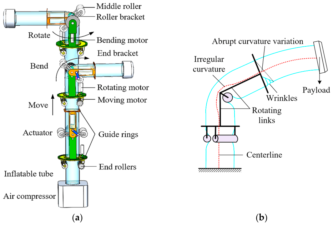
Figure 1a presents the system architecture and locomotion modes of the inflatable tube robot. The moving motor drives an end roller, and the friction generated between the three circumferentially arranged end rollers and tube wall enables the actuator to move freely along the tube. The rotation motor transfers torque to the base of the lower rotating link through a gear mechanism, thereby realizing tube rotation. The bending motor delivers torque to the guide rings through a bevel gear drive, inducing tube bending. The middle roller compresses the tube wall to form a local indentation for shaping control.

Under large bending compression loads, as shown in Figure 1b, the inflatable tube exhibits irregular deformation within the actuator, accompanied by a significant deviation in the outer tube’s centerline from the actuator’s midpoint line. Specifically, an abrupt curvature variation and local wrinkling appear near the tube root under large loads. These phenomena, together with the geometric asymmetry of the rigid mechanism, deformation lag, and potential buckling behavior, highlight the necessity of incorporating such effects into the mathematical model.

3. Static Model of Inflatable Membrane Tubes

Based on the principle of virtual work, a mapping is established from driven variables (motor moving torque ${\tau }_m$, rotation torque ${\tau }_{\varphi }$, and bending torque ${\tau }_{\theta }$) and loads to the actuation variables (actuator rotation angle ${\varphi }_a$, bending angle ${\theta }_a$, and moving arc length ${\mathcal{l}}_a$). Hawkes et al. [7] derived the eversion growth force of vine robots as a function of the path length and curvature, expressed as follows:

$${\left(pA\right)}_{eversion}=YA+{\left(1/\lambda v\right)}^{1/n}A+{\mu }_{r}w{\mathcal{l}}_a+C{e}^{{\mu }_{\theta }\theta },$$

(1)

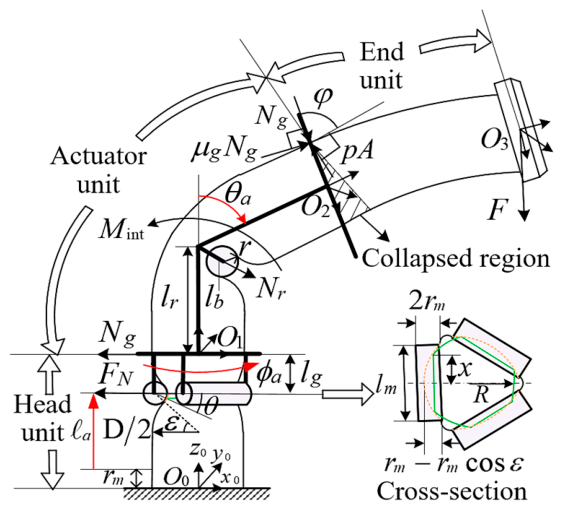
where $p$ is the internal pressure. $A$ is the cross-sectional area. $Y$ denotes the yield pressure required for tube material eversion. $\lambda$ is the material extensibility, and $v$ is the tip velocity. ${\mu }_r$ denotes the path length-dependent friction coefficient [56], and $w$ denotes the normal force exerted per unit length by the robot’s growing component. C is a fitting constant [56], and ${\mu }_{\theta }$ is the friction coefficient associated with the tube bending angler $\theta$ [56]. In Figure 2, $\theta ={\theta }_a-\phi$, where $\phi$ denotes the angle between the tube wall and upper guide ring surface, as defined in Equation (18). The eversion growth force considered in this work is provided by the moving torque. At low growth velocities, Equation (1) yields

$${\tau }_m\delta {\theta }_m=\left({\mu }_r{F}_N+C{e}^{{\mu }_{\theta }\theta }\right)\delta {\mathcal{l}}_a,$$

(2)

where ${\theta }_m$ is the rotation angle of the end rollers. The normal force exerted by the inflatable tube on the end roller can be denoted as $F_N=wf\left({\mathcal{l}}_a\right)$. Based on Hawkes et al. [7], $f\left({\mathcal{l}}_a\right)={\mathcal{l}}_a$. As shown in Figure 2, the normal force exerted per unit length is written as follows:

$$w=2p{\displaystyle {\int }_0^{\epsilon }\cos \theta dS}=2p{\displaystyle {\int }_0^{\arccos \left(\mathrm{D}/\left(2r_m+\mathrm{D}\right)\right)}\cos \theta dS},$$

(3)

where $\mathrm{D}$ represents the tube diameter. $r_m$ represents the end roller radius. From Figure 2, the cross-sectional area at angle $\theta$ can be deduced as follows:

$$S=R^2\left(\pi -3\arccos \left(\left(\mathrm{D}/2-r_m\cos \theta \right)/R\right)\right)+3x\left(\mathrm{D}/2-r_m\cos \theta \right),$$

(4)

where $R=\sqrt{x^2+{\left(\mathrm{D}/2-r_m\cos \theta \right)}^2}$. The contact region between the tube and end roller is elliptical, with a semi-major axis length $l_m/2$ and a semi-minor axis length $r_m-r_m\cos \epsilon$. $l_m$ is the end roller length. For the intersection line between this ellipse and the cross-section at angle $\theta$, the horizontal coordinate is $x=l_m/2\sqrt{1-{\left(1-\cos \theta \right)}^2{\left(r_m+\mathrm{D}/2\right)}^2/r_m^2}$.

Moreover, as depicted in Figure 2, the work performed by the rotational torque equals the work performed by the frictional torque, leading to the following equation:

$${\tau }_{\varphi }\delta {\varphi }_a=2{\mu }_g{N}_g{L}_g\delta \varphi +{\mu }_r{N}_r{L}_r\delta \varphi ,$$

(5)

where ${\mu }_g$ is the friction coefficient at the guide rings. The moment arms are $L_g=\mathrm{D}/2$ and $L_r=\sqrt{l_r^2+{\left(l_b-r\right)}^2-2l_r\left(l_b-r\right)\sin \left({\theta }_a/2\right)}$. $l_r$ is the length of the rotating link, $l_b$ denotes the middle roller bracket length, and $r$ is the middle roller radius. $\varphi$ is the tube rotation angle. $N_g$ denotes the normal force exerted by the tube on the guide ring, expressed as follows:

$$N_g=2T\sin \left(\left(\pi /2-\phi \right)/2\right)+2p\pi \mathrm{D}{d}_g,$$

(6)

where the tension is $T=p\pi {\mathrm{D}}^2/4$. $d_g$ is the width of the guide rings. As compression from the middle roller directly induces indentation of the tube, the normal force $N_r$ exerted by the tube on the roller [13], derived in [12], is written as follows:

$$N_r=pdV/dh,$$

(7)

where the volume change $dV$ and the tube clearance variation $dh$ induced by bending are solved via Equations (13) and (16).

Due to hysteresis between tube deformation and upper guide ring rotation, the tension-side membrane slides out by arc length ${\mathcal{l}}_s$. The bending torque work is governed by frictional dissipation and elastic deformation energy [57,58].

$${\tau }_{\theta }\delta {\theta }_a-{\mu }_g{N}_g\left(\phi \right){\mathcal{l}}_s+p{\displaystyle \frac{dV}{d\theta }}\delta {\theta }_a=0,$$

(8)

4. Kinematics of the Inflatable Tube Robot

Based on the PCC model’s segmented concept [6], the tube is divided into initial, actuator and end units (see Figure 2). The initial tube end is coaxially fixed to the actuator’s lower guide ring. At sufficient pressure, the initial unit centerline remains vertical with a constant cross-section. Within the actuator unit, the inner tube exhibits irregular curvature, while the outer tube centerline deviates from the actuator’s midpoint line. Under end-effector gravity, wrinkling at the end unit root causes curvature discontinuity. Outside the collapsed region, the tube deformation follows classical beam theory.

4.1. Robot Unit Kinematics

4.1.1. Actuator Unit Kinematics Under Bending and Indentation

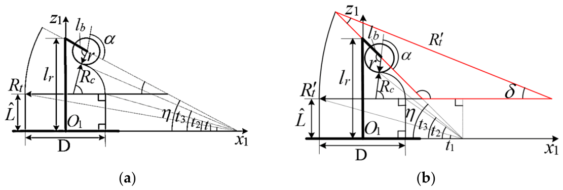
Under small bending (Figure 3a), tube deformation is governed primarily by bending loads. Under large bending (Figure 3b), compression dominates. For clarity of description, we define $\eta ={\theta }_a/2$. The boundaries of the angular parameter $\theta$ for the tensile (left) and compressive (right) paths of the tube are derived as follows:

$$\left\{\begin{array}{l}{t}_1=\arctan \left(\widehat{L}/\left[l_r\cot \eta +\mathrm{D}/2\right]\right)\hfill \\ t_2=\arctan \left(\widehat{L}/\left[l_r\cot \eta -\mathrm{D}/2\right]\right)\hfill \\ t_3=\arctan \left(\left[\widehat{L}+R_c\sin \left(\alpha -\eta \right)\right]/\sqrt{r^2+l_c^2+2r{l}_c\cos \alpha }\right)\hfill \end{array}\right.,$$

(9)

As illustrated in Figure 3a,b, the left path consists of a straight segment and a circular arc with radius $R_t$ or ${R^{\prime }}_t$, while the right path is composed of a straight segment, a circular arc with radius $R_c$, and a circular arc with radius $r$. Based on the geometric relationships in Figure 3, the x-coordinates of the paths in the local coordinate system are:

$$x_t=\left\{\begin{array}{ll}-\mathrm{D}/2\hfill & \theta \in \left[0,\right.\left.t_1\right)\hfill \\ R_t-\mathrm{D}/2-R_t\cos \left(\arcsin \left(\sin \theta /R_t\left(\widehat{L}\cot t_1-R_t-\widehat{L}\cot \theta \right)\right)+\theta \right)\hfill & \theta \in \left[t_1,\eta \right]\hfill \end{array}\right.,$$

(10)

$$x_c=\left\{\begin{array}{ll}\mathrm{D}/2\hfill & \theta \in \left[0,t_2\right)\hfill \\ \mathrm{D}/2-R_c+R_c\cos \left(\arcsin \left(\sin \theta /R_c\left(\widehat{L}\cot t_2+R_c-\widehat{L}\cot \theta \right)\right)-\theta \right)\hfill & \theta \in \left[t_2,t_3\right)\hfill \\ l_r\cot \eta -l_c\cos {\theta }_a+r\cos \left(\arcsin \left(\sin \theta /r\left[l_c\cos {\theta }_a-l_c\sin \eta \cot \theta \right]\right)-\theta \right)\hfill & \theta \in \left[t_3,\eta \right]\hfill \end{array}\right.,$$

(11)

where $l_c=l_r/\sin \eta -l_b$. $\widehat{L}$, $R_t$, $R_c$ and $\alpha$ are obtained via the geometric relationships in Figure 3. The paths have equal lengths, and drawing perpendicular lines from their starting points to the symmetry axis yields a geometric constraint [12]. The law of sines relates the angle $\delta$ and radius ${R^{\prime }}_t$ under large bending compression conditions.

$$\left\{\begin{array}{l}\left(2l_r-{\mathcal{l}}_s\right)/2=\widehat{L}+R_c\left(\alpha -\eta \right)+r\alpha =\widehat{L}+R_t\eta =\widehat{L}+{R^{\prime }}_t\delta \hfill \\ \begin{array}{l}\left(l_r\cot \eta -\mathrm{D}/2\right)\sin \eta =\left(r+R_c\right)\sin \alpha -R_c\sin \eta +\widehat{L}\cos \eta \\ \hfill =\widehat{L}/\sin t_1\sin \left(\eta -t_1\right)+\left(\widehat{L}-\mathrm{D}\right)\cos \eta \end{array}\hfill \\ {R^{\prime }}_t/\sin \left(\pi -\eta \right)=\left({R^{\prime }}_t-\widehat{L}\cot t_1+\widehat{L}\cot \eta \right)/\sin \left(\eta -\delta \right)\hfill \end{array}\right.,$$

(12)

where ${\mathcal{l}}_s$ is dependent on the bending angle, which can be obtained experimentally.

Based on Equations (10) and (11), the tube path clearance is derived as follows:

$$h=\left(x_c-x_t\right)/\cos \theta ,$$

(13)

Assuming the cross-sectional perimeter remains constant, the semi-major axis length of the cross-section at the bracket is obtained using Ramanujan’s approximation formula:

$$a=\mathrm{D}/2-h/3+\sqrt{3}\mathrm{D}/6\sqrt{3-4h/\mathrm{D}+4h^2/{\mathrm{D}}^2-h^3/{\mathrm{D}}^3},$$

(14)

From Figure 3, the arc length of the central path is deduced as follows:

$$\mathcal{l}\left(\theta \right)=\sqrt{{\left(d\left(x_c+x_t\right)/d\theta \right)}^2+{\left(d\left(\left(x_c-x_t\right)\tan \theta \right)/d\theta \right)}^2},$$

(15)

From Equations (12)–(14), the tube volume change is expressed as follows:

$$dV=\pi {\mathrm{D}}^2/2\mathcal{l}\left({\theta }_a/2\right)-2{\displaystyle {\int }_0^{{\theta }_a/2}\pi ah\frac{d\mathcal{l}\left(\theta \right)}{d\theta }d\theta },$$

(16)

The restoring moment generated by internal pressure is $M_r=\pi p{\left(ah/2\right)}^{3/2}$. Based on the approach of Hawkes et al. [7], the moment balance equation is

$$M_{\mathrm{int}}=N_g\left[l_r+\left(h/2+r+l_b\right)\sin \left({\theta }_a/2\right)\right]-{\mu }_g{N}_g\left[\mathrm{D}/2-\left(h/2+r+l_b\right)\cos \left({\theta }_a/2\right)\right],$$

(17)

Substituting Equation (6) into Equation (17) yields

$$\phi ={\displaystyle \frac{\pi }{2}}-2\arcsin \left({\displaystyle \frac{ah\sqrt{ah/2}/{\mathrm{D}}^2}{\left[l_r+\left(h/2+r+l_b\right)\sin \left({\theta }_a/2\right)\right]-{\mu }_g\left[\mathrm{D}/2-\left(h/2+r+l_b\right)\cos \left({\theta }_a/2\right)\right]}}-{\displaystyle \frac{4d_g}{\mathrm{D}}}\right),$$

(18)

4.1.2. End Unit Kinematics Under Wrinkling

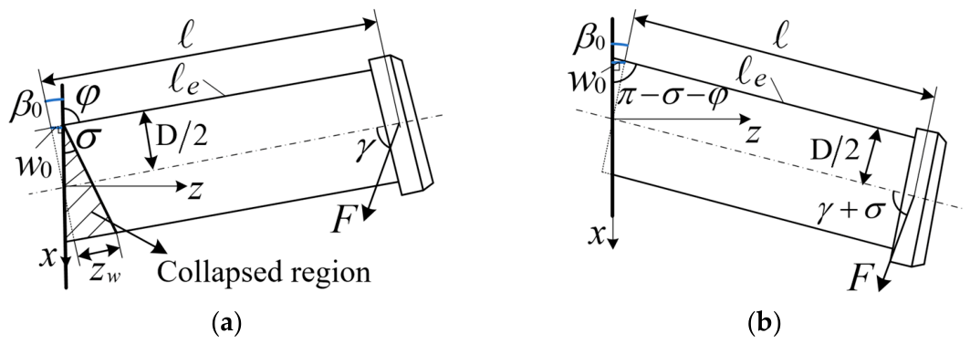
In Figure 4a, $\gamma ={\theta }_a-\phi$ denotes the initial deflection angle between the payload and axial direction of the end unit. $\mathcal{l}$ is the equivalent arc length of the end unit. The bending moment of the cross-section at the coordinate $z\in \left[0,\mathcal{l}\right]$ in the local coordinate system is deduced as follows:

$$M\left(z\right)=F\sin \gamma \left(\mathcal{l}-z\right)+F\cos \gamma \left(v\left(\mathcal{l}\right)-v\left(z\right)\right),$$

(19)

Based on membrane theory [8], the wrinkling moment and failure moment are $M_w=\pi p{\mathrm{D}}^3/16$, and $M_{cr}=\pi p{\mathrm{D}}^3/8$, respectively. Based on Equation (19), the wrinkling and failure criteria of the cantilevered tube can be defined as:

$$\left\{\begin{array}{ll}M\left(0\right)<M_w\hfill & no wrinkling\hfill \\ M\left(0\right)=M_w\hfill & wrinkling\hfill \\ M\left(0\right)\ge M_{cr}\hfill & failure\hfill \end{array}\right.,$$

(20)

IAs shown in Figure 4, the deflection angle and deflection of the cross-section at coordinate z are $\beta \left(z\right)$ and $v\left(z\right)$. Based on the modified Timoshenko beam theory [43],

$$\left\{\begin{array}{l}\beta \left(z\right)=\mathrm{A}{e}^{\mathsf{\Omega }z}+\mathrm{B}{e}^{-\mathsf{\Omega }z}+{\delta }_1\hfill \\ v\left(z\right)={\displaystyle \frac{1}{\mathsf{\Omega }}}{\displaystyle \frac{K{G}^{\ast }{S}^{\ast }+P}{K{G}^{\ast }{S}^{\ast }}}\left(\mathrm{A}{e}^{\mathsf{\Omega }z}-\mathrm{B}{e}^{-\mathsf{\Omega }z}\right)+{\displaystyle \frac{K{G}^{\ast }{S}^{\ast }}{K{G}^{\ast }{S}^{\ast }-P}}{\delta }_{1}z+{\delta }_2\hfill \end{array}\right.,$$

(21)

where $\mathsf{\Omega }=P/\sqrt{K{E}^{\ast }{I}^{\ast }{G}^{\ast }{S}^{\ast }}$. $P=p\pi {\mathrm{D}}^2/4$ is the pressure force. $K$ is the shear coefficient in Cowper’s theory [59]. $t$ is the tube thickness. $E$ is the Young’s modulus. $G$ is the shear modulus. $I$ denotes the second moment. $E^{\ast }=Et$, $I^{\ast }=It$, $G^{\ast }=Gt$, and $S^{\ast }=\pi {\mathrm{D}}^2/4t$. ${\delta }_1=F_{bc}\left(K{G}^{\ast }{S}^{\ast }-P\right)/P^2$. The shear stress equation implies $F_{bc}=F\sin \gamma$. Based on the boundary conditions $v\left(0\right)=v_0$, $\beta \left(0\right)={\beta }_0$, and $M\left(\mathcal{l}\right)=0$, it can be obtained as follows:

$$\left\{\begin{array}{l}\mathrm{A}=\left({\beta }_0+F_{bc}{\displaystyle \frac{P-K{G}^{\ast }{S}^{\ast }}{P^2}}\right){\displaystyle \frac{e^{-\mathsf{\Omega }\mathcal{l}}}{2ch\mathsf{\Omega }\mathcal{l}}}=\mathrm{B}{e}^{-2\mathsf{\Omega }\mathcal{l}}\hfill \\ {\delta }_2=v_0-{\displaystyle \frac{1}{\mathsf{\Omega }}}{\displaystyle \frac{K{G}^{\ast }{S}^{\ast }+P}{K{G}^{\ast }{S}^{\ast }}}\left({\beta }_0+F_{bc}{\displaystyle \frac{P-K{G}^{\ast }{S}^{\ast }}{P^2}}\right){\displaystyle \frac{e^{-\mathsf{\Omega }\mathcal{l}}-e^{\mathsf{\Omega }\mathcal{l}}}{2ch\mathsf{\Omega }\mathcal{l}}}\hfill \end{array}\right.,$$

(22)

Substituting Equation (22) into Equation (21), the solution can be derived as follows:

$$\left\{\begin{array}{l}\beta \left(z\right)={\beta }_0{\displaystyle \frac{ch\mathsf{\Omega }\left(\mathcal{l}-z\right)}{ch\mathsf{\Omega }\mathcal{l}}}+F_{bc}{\displaystyle \frac{P-K{G}^{\ast }{S}^{\ast }}{P^2}}{\displaystyle \frac{ch\mathsf{\Omega }\left(\mathcal{l}-z\right)-ch\mathsf{\Omega }\mathcal{l}}{ch\mathsf{\Omega }\mathcal{l}}}\hfill \\ v\left(z\right)=v_0+\left({\beta }_0+F_{bc}{\displaystyle \frac{K{G}^{\ast }{S}^{\ast }-P}{P^2}}\right){\displaystyle \frac{K{G}^{\ast }{S}^{\ast }+P}{K{G}^{\ast }{S}^{\ast }\mathsf{\Omega }}}{\displaystyle \frac{sh\mathsf{\Omega }\left(\mathcal{l}-z\right)-sh\mathsf{\Omega }\mathcal{l}}{ch\mathsf{\Omega }\mathcal{l}}}+{\displaystyle \frac{K{G}^{\ast }{S}^{\ast }}{P^2}}{F}_{bc}z\hfill \end{array}\right.,$$

(23)

where ${\beta }_0$, $v_0$ and $\mathcal{l}$ when the cantilevered tube is unstressed (Figure 4a) are deduced as follows:

$$\left\{\begin{array}{l}{\beta }_0=\pi /2-\phi \hfill \\ v_0=\mathrm{D}/2\sin {\beta }_0=\mathrm{D}/2\cos \phi \hfill \\ \mathcal{l}={\mathcal{l}}_e+\mathrm{D}/2\tan {\beta }_0={\mathcal{l}}_e+\mathrm{D}/2\cot \phi \hfill \end{array}\right.,$$

(24)

where ${\mathcal{l}}_e$ denotes the arc length of the end unit. In addition, ${\beta }_0$, $v_0$ and $\mathcal{l}$ when the tube root collapses (Figure 4b) are derived as follows:

$$\left\{\begin{array}{l}{\beta }_0=\sigma +\phi -\pi /2\hfill \\ v_0=\mathrm{D}/2\sin {\beta }_0=-\mathrm{D}/2\cos \left(\sigma +\phi \right)\hfill \\ \mathcal{l}={\mathcal{l}}_e-\mathrm{D}/2\tan {\beta }_0={\mathcal{l}}_e+\mathrm{D}/2\cot \left(\sigma +\phi \right)\hfill \\ F_{bc}=F\sin \left(\gamma +\sigma \right)\hfill \end{array}\right.,$$

(25)

where the angle $\sigma$ can be solved via Equations (26) and (27). Set ${\beta }_0=v_0=0$ and substitute them into Equation (23) to obtain $v\left(\mathcal{l}\right)$ and $v\left(z\right)$. Then, substituting the results and the wrinkling moment into Equation (19) yields a transcendental equation as follows:

$$\begin{array}{l}\left(1+{\displaystyle \frac{K{G}^{\ast }{S}^{\ast }}{P^2}}F\cos \left({\theta }_a-\phi \right)\right)z+F\cos \left({\theta }_a-\phi \right){\displaystyle \frac{K^2{G}^{\ast 2}{S}^{\ast 2}-P^2}{P^{2}K{G}^{\ast }{S}^{\ast }\mathsf{\Omega }}}{\displaystyle \frac{sh\mathsf{\Omega }\left(\mathcal{l}-z\right)-sh\mathsf{\Omega }\mathcal{l}}{ch\mathsf{\Omega }\mathcal{l}}}\\ \hfill =-{\displaystyle \frac{\pi p{\mathrm{D}}^3}{16F\sin \left({\theta }_a-\phi \right)}}+\mathcal{l}+v\left(\mathcal{l}\right)\cot \left({\theta }_a-\phi ,\right)\end{array}$$

(26)

Solving Equation (26) via the Newton–Raphson method gives the initial wrinkling position $z=z_w$. Using the law of sines and law of cosines, the angle $\sigma$ is obtained as follows:

$$\sigma =\arcsin {\displaystyle \frac{\left(\mathrm{D}/2\cos \phi +z_w\right)\sin \phi }{\sqrt{{\left(\mathrm{D}/\sin \phi \right)}^2+{\left(\mathrm{D}/2\cos \phi +z_w\right)}^2-2\mathrm{D}/\sin \phi \left(\mathrm{D}/2\cos \phi +z_w\right)\cos \phi }}},$$

(27)

Equation (24) is substituted into Equation (23) to obtain the deflection angle ${\beta }_{nf}\left(z\right)$ and deflection $v_{nf}\left(z\right)$ under the non-collapsed condition. Equation (25) is substituted into Equation (23) to derive the deflection angle ${\beta }_f\left(z\right)$ and deflection $v_f\left(z\right)$ under the collapsed condition. This resolves the curvature variation at root wrinkling in the cantilever tube.

4.2. Segmental Kinematic Modeling of the Inflatable Tube Robot

The forward kinematics [5] of the robotic system is defined as a mapping from the actuator state $\mathit{q}={\left[\begin{array}{ccc}{\varphi }_a& {\theta }_a& {\mathcal{l}}_a\end{array}\right]}^T$ to the configuration state $\mathit{g}={\left[\begin{array}{ccc}\varphi & \theta & \mathcal{l}\end{array}\right]}^T$ and then to the task state $\mathit{X}={\left[\begin{array}{llllll}x\hfill & y\hfill & z\hfill & {\theta }_x\hfill & {\theta }_y\hfill & {\theta }_z\hfill \end{array}\right]}^T$. $\mathit{X}$ denotes the absolute coordinate vector of the centerline points. In Figure 2, $\mathit{g}$ is divided into the configuration state ${\mathit{g}}_k=$${\left[\begin{array}{ccc}{\varphi }_k& {\theta }_k& {\mathcal{l}}_k\end{array}\right]}^T$ of the unit k (k = 1, 2, 3). Given the actuator state, ${\mathit{g}}_k$ can be expressed as follows:

$${\mathit{g}}_1={\left[\begin{array}{ccc}0& 0& {\mathcal{l}}_1\end{array}\right]}^T={\left[\begin{array}{ccc}0& 0& r_m+{\mathcal{l}}_a+l_g\end{array}\right]}^T,$$

(28)

$${\mathit{g}}_2={\left[\begin{array}{ccc}{\varphi }_2& {\theta }_2& {\mathcal{l}}_2\end{array}\right]}^T={\left[\begin{array}{ccc}{\varphi }_a& {\theta }_a-\phi & 2\mathcal{l}\left({\theta }_a/2\right)\end{array}\right]}^T,$$

(29)

$${\mathit{g}}_3={\left[\begin{array}{ccc}{\varphi }_3& {\theta }_3& {\mathcal{l}}_3\end{array}\right]}^T=\left\{\begin{array}{ll}{\left[\begin{array}{ccc}0& {\beta }_{nc}\left(\mathcal{l}\right)& \mathcal{l}\end{array}\right]}^T\hfill & no collapse\hfill \\ {\left[\begin{array}{ccc}0& {\beta }_c\left(\mathcal{l}\right)& \mathcal{l}\end{array}\right]}^T\hfill & collapse\hfill \end{array}\right.,$$

(30)

where ${\mathcal{l}}_e=L-{\mathcal{l}}_1-{\mathcal{l}}_2$. $L$ denotes the total tube length.

As depicted in Figure 2, $O_{k-1}{x}_{k-1}{y}_{k-1}{z}_{k-1}$ is the base frame of unit k. The rotation and transformation matrices of the frame $O_k{x}_k{y}_k{z}_k$ relative to the previous frame are given by:

$${\mathit{R}}_k=\left[\begin{array}{ccc}\cos {\varphi }_k\left(\cos {\theta }_k-1\right)+1& \sin {\varphi }_k\cos {\varphi }_k\left(\cos {\theta }_k-1\right)& \cos {\varphi }_k\sin {\theta }_k\\ \sin {\varphi }_k\cos {\varphi }_k\left(\cos {\theta }_k-1\right)& {\cos }^2{\varphi }_k\left(1-\cos {\theta }_k\right)+\cos {\theta }_k& \sin {\varphi }_k\sin {\theta }_k\\ -\cos {\varphi }_k\sin {\theta }_k& -\sin {\varphi }_k\sin {\theta }_k& \cos {\theta }_k\end{array}\right],$$

(31)

$${\mathit{O}}_k=\left\{\begin{array}{ll}{\mathcal{l}}_k/{\theta }_k{\left[\begin{array}{ccc}\cos {\varphi }_k\left(1-\cos {\theta }_k\right)& \sin {\varphi }_k\left(1-\cos {\theta }_k\right)& \sin {\theta }_k\end{array}\right]}^T\hfill & {\theta }_k\ne 0\hfill \\ {\left[\begin{array}{ccc}0& 0& {\mathcal{l}}_k\end{array}\right]}^T\hfill & {\theta }_k=0\hfill \end{array}\right.,$$

(32)

The homogeneous transformation matrix of the robotic system is derived as follows:

$$\mathit{H}=\left[\begin{array}{cc}{\mathit{R}}_0& {\mathit{O}}_0\\ {\mathbf{0}}_{1\times 3}& 1\end{array}\right]\left[\begin{array}{cc}{\mathit{R}}_1& {\mathit{O}}_1\\ {\mathbf{0}}_{1\times 3}& 1\end{array}\right]\dots \left[\begin{array}{cc}{\mathit{R}}_3& {\mathit{O}}_3\\ {\mathbf{0}}_{1\times 3}& 1\end{array}\right]=\left[\begin{array}{cccc}{h}_1& h_4& h_7& h_{10}\\ h_2& h_5& h_8& h_{11}\\ h_3& h_6& h_9& h_{12}\\ 0& 0& 0& 1\end{array}\right],$$

(33)

where ${\mathit{R}}_0$ and ${\mathit{O}}_0$ are the rotation and transformation matrices of the starting point ${\mathit{X}}_0$ with respect to the world frame. The position vector of ${\mathit{X}}_0$ is defined as ${\mathit{x}}_0={\left[\begin{array}{ccc}{x}_0& y_0& z_0\end{array}\right]}^T$. ${\mathit{O}}_0={\mathit{x}}_0$. ${\mathit{R}}_0$ has the same form as ${\mathit{R}}_k$, with angles defined as ${\theta }_0=\arctan \left(\sqrt{x_0^2+y_0^2}/z_0\right)$, and ${\varphi }_0=\arctan \left(y_0/x_0\right)$. Based on [5] and Rodrigues’ rotation formula [60], the task state is

$$\mathit{X}={\left[\begin{array}{llllll}{h}_{10}\hfill & h_{11}\hfill & h_{12}\hfill & \arctan \left(-h_8/h_9\right)\hfill & \arctan \left(h_7/h_9\right)\hfill & \arctan \left(h_8/h_7\right)\hfill \end{array}\right]}^T,$$

(34)

Algorithm 1 details the modeling procedure for the inflatable tube robot.

Algorithm 1: Static Parameter Identification and Kinematic Modeling.

$\mathbf{Input}\mathbf{:} \mathrm{Driven} \mathrm{variables} {\tau }_m$$, {\tau }_{\varphi }$$, {\tau }_{\theta }$ internal pressure $p$, payload $F$$, \mathrm{actuation} \mathrm{variables} {\varphi }_a$$, {\theta }_a$$, {\mathcal{l}}_a$$, \mathrm{physical} \mathrm{parameters} l_r$, $r$$, \mathrm{D}, l_b$$, d_g$$, r_m$$, l_m$$, l_g$, $L$$, K, G, t, \mathrm{and} \mathrm{starting} \mathrm{position} \mathrm{vector} {\mathit{x}}_0$

$\mathbf{Output}\mathbf{:} \mathrm{Static} \mathrm{parameters} {\mu }_r$, $C$$, {\mu }_{\theta }$$, {\mu }_g$, and end-effector pose $\mathit{X}$

1:   Compute $\widehat{L}$$, R_t$$, R_c$, $\alpha$$, {R^{\prime }}_t$$\mathrm{using} \mathrm{Equation} \left(12\right) \mathrm{with} {\theta }_a$, D, $r$.

$2:\hspace{1em} \mathrm{Compute} x_t$$, x_c$ using Equations (10) and (11) with $\widehat{L}$$, R_t$$, R_c$, $\alpha$$, {R^{\prime }}_t$.

$3:\hspace{1em} h\leftarrow \left(x_c-x_t\right)/\cos \theta$$; a\leftarrow \mathrm{D}/2-h/3+\sqrt{3}\mathrm{D}/6\sqrt{3-4h/\mathrm{D}+4h^2/{\mathrm{D}}^2-h^3/{\mathrm{D}}^3}$;

4:   Compute $\phi$ using Equation (18) with $a$, $h$$, \mathrm{D}, l_r$, $r$$, l_b$$, {\theta }_a$$, d_g$.

$5:\hspace{1em} \mathrm{Fit} {\mu }_r$$, f\left({\mathcal{l}}_a\right)$, $C$$, {\mu }_{\theta }$$\mathrm{using} \mathrm{Equations} \left(2\right)–\left(4\right) \mathrm{with} l_m$$, r_m$, D, $p$$, {\tau }_m$$, {\theta }_m$, $\phi$$, {\theta }_a$$, {\mathcal{l}}_a$.

$6:\hspace{1em} \mathcal{l}\left(\theta \right)\leftarrow \sqrt{{\left(d\left(x_c+x_t\right)/d\theta \right)}^2+{\left(d\left(\left(x_c-x_t\right)\tan \theta \right)/d\theta \right)}^2}$;

7:   $dV\leftarrow \pi {\mathrm{D}}^2/2\mathcal{l}\left({\theta }_a/2\right)-2{\int }_0^{{\theta }_a/2}\pi ahd\mathcal{l}(\theta )/d\theta d\theta$;

$8:\hspace{1em} N_r\leftarrow pdV/dh;N_g\leftarrow p\pi {\mathrm{D}}^2/2\sin ((\pi /2-\phi )/2)+2p\pi \mathrm{D}{d}_g;$

$9:\hspace{1em} \mathrm{Fit} {\mu }_g$$\mathrm{using} \mathrm{Equation} \left(5\right) \mathrm{with} {\tau }_{\varphi }$$, {\varphi }_a$$, N_g$$, \mathrm{D}, {\mu }_r$$, N_r$$, l_r$, $r$$, l_b$.

$10:\hspace{1em} \mathrm{Fit} {\tau }_{\theta }$$\mathrm{using} \mathrm{Equation} \left(8\right) \mathrm{with} {\theta }_a$$, {\mu }_g$$, N_g$, $p$$, {\theta }_a$$, dV$.

$11:\hspace{1em} {\mathit{g}}_1\leftarrow {\left[\begin{array}{ccc}0& 0& r_m+{\mathcal{l}}_a+l_g\end{array}\right]}^T$$;{\mathit{g}}_2\leftarrow {\left[\begin{array}{ccc}{\varphi }_a& {\theta }_a-\phi & 2\mathcal{l}\left({\theta }_a/2\right)\end{array}\right]}^T$;

$12:\hspace{1em} \mathrm{Compute} {\beta }_0$$, v_0$, $\mathcal{l}$ using Equation (24) with $\phi$, D, $L$$, {\mathit{g}}_1$$, {\mathit{g}}_2$.

$13:\hspace{1em} \mathrm{Compute} v\left(\mathcal{l}\right)$$\mathrm{using} \mathrm{Equation} \left(23\right) \mathrm{with} v_0$$, {\beta }_0$, $F$, $\phi$$, {\theta }_a$, $p$, D, K, G, t, $\mathcal{l}$.

$14:\hspace{1em} M\left(0\right)\leftarrow F\sin \left({\theta }_a-\phi \right)\mathcal{l}+F\cos \left({\theta }_a-\phi \right)v\left(\mathcal{l}\right)$;

$15:\hspace{1em} \mathbf{if} M\left(0\right)<M_{cr}=p\pi {\mathrm{D}}^3/8$$\mathbf{then} \mathrm{Compute} {\beta }_{nc}\left(\mathcal{l}\right)$ using Equation (23).

$16:\hspace{1em}\hspace{1em}{\mathit{g}}_3\leftarrow {\left[\begin{array}{ccc}0& {\beta }_{nc}\left(\mathcal{l}\right)& \mathcal{l}\end{array}\right]}^T$;

17:   else

18:    Compute $\sigma$ using Equations (26) and (27) with K, G, t, D, $p$, $F$, $\phi$$, {\theta }_a$, $\mathcal{l}$.

$19:\hspace{1em}\hspace{1em}\hspace{1em}\mathrm{Compute} {\beta }_0$, $\mathcal{l}$$, F_{bc}$ using Equation (25) with $\sigma$, $\phi$, D, $L$$, {\mathit{g}}_1$$, {\mathit{g}}_2$, $F$.

$20:\hspace{1em}\hspace{1em}\hspace{1em}\mathrm{Compute} {\beta }_c\left(\mathcal{l}\right)$$\mathrm{using} \mathrm{Equation} \left(23\right) \mathrm{with} {\beta }_0$, $\mathcal{l}$$, F_{bc}$, $\phi$$, {\theta }_a$, $p$, D, K, G, t, $\mathcal{l}$.

$21:\hspace{1em}\hspace{1em}{\mathit{g}}_3\leftarrow {\left[\begin{array}{ccc}0& {\beta }_c\left(\mathcal{l}\right)& \mathcal{l}\end{array}\right]}^T$;

22:   Compute $\mathit{X}$$\mathrm{using} \mathrm{Equations} \left(31\right)–\left(34\right) \mathrm{with} {\mathit{g}}_1$$, {\mathit{g}}_2$$, {\mathit{g}}_3$$, {\mathit{x}}_0$.

5. Experiments and Results

5.1. Experimental Setup

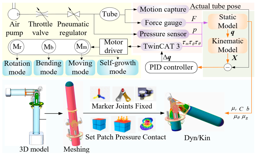
Figure 5 shows the main components of the robotic system, including a pneumatic supply system, a thermoplastic polyurethane (TPU) membrane tube, and an actuator. The pneumatic supply system consists of an air pump (FB550DO-10A25, Taizhou Feibao Air Compressor Co., Ltd., Wenling, China, 0.7 MPa) integrated with a pressure regulator and a throttle valve. The actuator is driven by servo motors (DCX-19S, Maxon Motor AG, Sachseln, Switzerland, 12 V) with a maximum torque of 0.0115 N·m, and is controlled via the TwinCAT 3 development environment (Beckhoff Automation GmbH & Co. KG, Verl, Germany). The multi-sensor measurement system comprises a motion capture system (Prime 13, OptiTrack, Corvallis, OR, USA) for recording the tube curve, an SH-20 digital force sensor (±0.1 N, Sundoo Instruments, Wenzhou, China) for quantifying loads, and a pressure sensor (ZSE30AF, SMC Corporation, Tokyo, Japan, ±100 kPa, 0.1 kPa resolution) for monitoring of the internal pressure within the inflatable tube. The physical parameters of the inflatable tube robot are presented in

Table 1. Geometric robot data and contact property.

Parameter	Value	Description
L	1000 mm	Tube length
D	62 mm	Tube diameter
t	0.25 mm	Thickness
$l_m$	30 mm	End roller length
$r_m$	8 mm	End roller radius
$l_g$	20 mm	End roller bracket length
r	18 mm	Middle roller radius
$l_b$	50 mm	Middle roller bracket length
$l_r$	100 mm	Rotating link length
$d_g$	2 mm	Guide ring thickness

.

Experimental data measured by the multi-sensor system were employed to identify the static parameters. A rigid–flexible gas coupled simulation framework was established, incorporating a 3D model constructed in 3D modeling software. The TPU tube was meshed using ANSYS Workbench 19.0, while the complex interactions among the actuator, the inflatable TPU tube, and the payload were simulated via RecurDyn V9R2. The key parameters were configured as follows: Young’s modulus of 30 MPa, Poisson’s ratio of 0.4, contact stiffness of 1 × 10⁶ N/m, and viscous damping coefficient of 1 × 10³ N·s/m. The simulation results and experimental motion sequences of the robot are provided in the Supplementary Materials (Video S1).

5.2. Static Parameter Identification

To systematically evaluate the model prediction performance, we use cross-valid-ation on prototype experiments covering diverse operating conditions: internal pressure (8–14 kPa), bending angle (0–100°), moving arc length (0–400 mm), and external load (0–1.4 N). The experimental data are split into training and test sets: the training set is used for parameter fitting, while the test set validates the prediction accuracy.

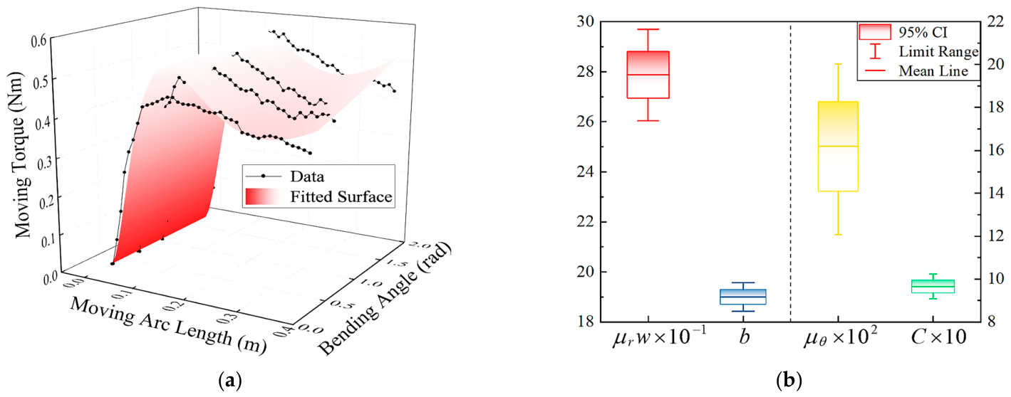
Based on experimental data obtained for bending angles ranging from 0° to 100° and moving arc lengths from 0 to 400 mm, $f\left({\mathcal{l}}_a\right)$ was modified as $e^{-b{\mathcal{l}}_a}{\mathcal{l}}_a$, leading to the derivation of Equation (1) as ${\tau }_m\delta {\theta }_m={\mu }_{r}w{e}^{-b{\mathcal{l}}_a}{\mathcal{l}}^{2a}+C{e}^{{\mu }_{\theta }\theta }{\mathcal{l}}_a$. When fitted at a bending angle of 0°, ${\mu }_{r}w$, $b$ and $C$ were obtained to be 303.92 ± 15.49, 21.68 ± 0.47, and 1.08 ± 0.02, respectively, with a coefficient of determination of R² = 0.9624, which shows excellent goodness of fit. Using these identified parameters as initial guesses, the improved moving torque was modeled as a fitting surface, as shown in Figure 6a. The fitting results for ${\mu }_{r}w$, $b$, $C$ and ${\mu }_{\theta }$ are shown in Figure 6b. The fitting surface yields an R² value of 0.926, suggesting a satisfactory and reliable fitting performance. Finally, in combination with the derived result ${\mu }_{r}w=278.75\pm 9.31$ and Equation (3), ${\mu }_r=54.00\pm 1.80$.

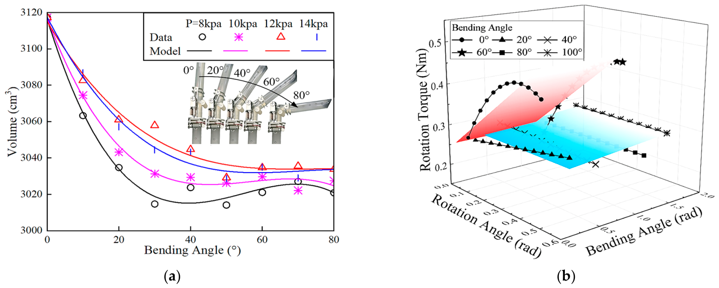
The actual volume and the volume described by Equation (15) are shown in Figure 7a. A comparison of the results indicates that the fitted curve of tube volume is highly reliable. When ${\theta }_a=0^{\circ }~{40}^{\circ }$, the indentation depth of the middle roller increases, resulting in a significant decrease in volume. When ${\theta }_a={40}^{\circ }~{60}^{\circ }$, wrinkles form on the membranes on both sides of the roller and gradually fold, leading to a slower volume change. Between 60° and 80°, the indentation depth remains constant, and the volume remains almost unchanged. When ${\theta }_a>{80}^{\circ }$, the volume continues to decrease slowly, as the membranes on both sides gradually wrap around the middle roller under large bending.

Based on the obtained volume and the experimental measurements, Equation (5) was fitted to the dataset. As shown in Figure 7a, the volume remains nearly constant under $p=12\mathrm{kPa}$ and ${\theta }_a=0^{\circ },{60}^{\circ }$. Following compensation for pressure fluctuations, the fitted surface for the rotation torque at ${\theta }_a=0^{\circ },{60}^{\circ }$ is shown in Figure 7b, with the initial value of ${\mu }_g$ obtained as 0.86 ± 0.07. After initializing the parameters in Equation (5), the fitted surface at ${\theta }_a={20}^{\circ },{40}^{\circ },{80}^{\circ },{100}^{\circ }$ is depicted in Figure 7b. The relative errors of the proposed rotation motor torque model are 8.92% and 3.38% for the two operating conditions, respectively, demonstrating that the model achieves excellent prediction accuracy for rotation motor torque of the inflatable robot.

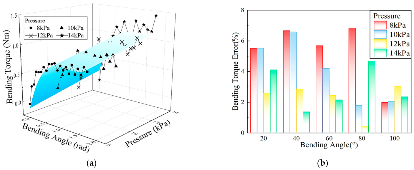
Based on the measured volume variation, Equation (8) was fitted to the dataset, yielding the fitted surface of the actuator’s bending motor torque shown in Figure 8a. The relative errors of the bending torque under different pressures are presented in Figure 8b. The relative errors of bending torque across all tested bending angles (0–100°) and pressures (8–14 kPa) are consistently below 7%, with most values remaining under 5%. These results show that our model achieves high accuracy and reliability in predicting the bending motor torque of the inflatable robot, thereby verifying its predictive power and generalization capability for practical engineering applications.

5.3. Kinematics Validation

5.3.1. End Unit Kinematic Validation

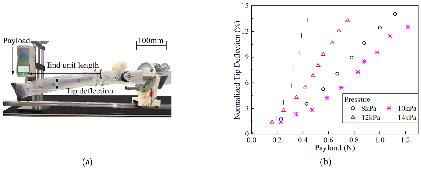
Static loading tests (Figure 9a) were conducted to characterize the load–deflection responses of inflatable tubes, with the results shown in Figure 9b. At low loads (0–0.2 N), the normalized tip deflection remains below 3% and increases linearly, showing good agreement with the modified Timoshenko beam theory [43]. In the medium-load regime (0.2–0.8 N), the deflection grows faster than the linear prediction, while at high loads (>0.8 N), it rises abruptly, accompanied by local wrinkling and buckling at the tube root. Furthermore, the tip deflection increases gently at low pressures (8, 10 kPa) but rises rapidly at high pressures (12, 14 kPa), exceeding 13% at 0.4 N under 14 kPa. High pressure pre-tensions the membrane, making the tube prone to buckling and wrinkling under large deformations. Given the critical role of high pressure and high load in load-bearing performance, investigating root curvature evolution under large loads is essential.

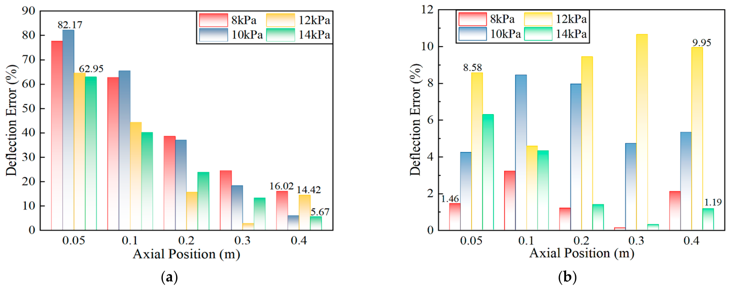
To evaluate the proposed end unit kinematic model’s prediction accuracy, Figure 10 shows the axial distribution of the relative deflection error for cantilever tubes under varying pressures. Timoshenko beam theory [42] yields substantial errors near the tube root across all pressures, peaking at 82.17% at 8 kPa. This discrepancy stems from its small deformation assumption, which fails to capture localized root wrinkling and buckling under large bending loads. In contrast, our model maintains excellent accuracy along the cantilever tube length, with errors consistently below 10% for all tested pressures. At the tip, errors are only 9.95% at 12 kPa and 1.19% at 14 kPa, outperforming the Timoshenko beam theory predictions of 14.42% and 5.67%, respectively. Moreover, the prediction error of Timoshenko beam theory [42] becomes more significant at higher pressures, further showing the superiority of the proposed model. These results confirm that the end unit kinematics model can provide reliable deflection predictions for inflatable actuators.

5.3.2. Robot-Level Kinematic Validation

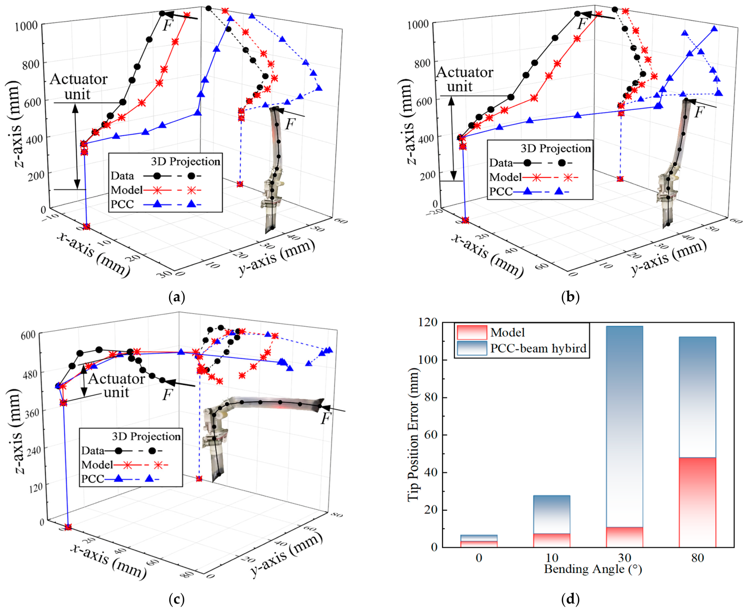
The kinematic performance of the robotic system was systematically validated through experiments at an internal pressure of 12 kPa, a rotation angle of 30°, and an applied load of 1.77 N in the negative x-axis direction, as shown in Figure 11.

The three-dimensional centerlines in Figure 11a–c demonstrate the tube centerline configurations under bending angles of 10°, 30°, and 80°, respectively. The PCC–beam hybrid method combines the PCC model [6] for the actuator unit with the modified Timoshenko beam theory [42] for the end unit. The results show that centerlines from the proposed model are closer to the actual curves than those from the PCC–beam hybrid method, in both the 3D view and x-z plane. In contrast, the hybrid method exhibits significant deviations from the actual curves, especially at large bending angles, where it fails to account for internal pressure, external loads, and complex deformation behaviors. Figure 11d shows a quantitative comparison of endpoint position errors at bending angles of 0°, 10°, 30°, and 80°. The relative error of the proposed model, normalized by the tube length, remains below 5% across the entire range of bending angles. The hybrid method error exceeds 11% at angles above 30°. This comparison directly demonstrates that the proposed model achieves a clear improvement in kinematic accuracy over conventional methods, with distinct advantages under large deformation conditions. The above findings validate the effectiveness of the proposed kinematic model, enabling the fast and accurate kinematic prediction of inflatable robots under large deformation conditions.

6. Discussion

This study presents an inflatable robotic system driven by pneumatic networks and servo motors, achieving 120° bending, 360° rotation, adaptive locomotion, and payload carrying capacity for environmental exploration. For inflatable tubes, the challenge of accurate modeling under coupled loading is addressed via a theoretical framework that integrates the virtual work principle and a segmented modeling strategy. The proposed models are supported by a solid theoretical foundation. Both models incorporate multiple parameters, including the physical properties of the tube material (Poisson’s ratio, elastic modulus, friction coefficient, etc.), geometric parameters (outer diameter, thickness, and length of the inflatable tube), and physical parameters of the actuator mechanism. Physical models of this type inherently have good generalization ability, and the comprehensive parameterization further improves model generalization.

Regarding the static modeling, we revise the path length-dependent term of the eversion growth force for vine robots, which was originally presented by Blumenschein et al. as a linear function of the path length, into an exponential form. Validation of this modified model on a multi-sensor platform shows that the fitting of the driving torque yields a coefficient of determination of 0.926. This result shows that the modified model achieves substantially improved agreement with the experimental torque measurements, thus strengthening the reliability of subsequent motion control. The introduction of a tunable coefficient b further enhances the model’s adaptability to various robot structures and working conditions, extending its flexibility in practical applications.

The identification results of the other static models exhibit favorable accuracy. Under two representative working conditions, the relative errors of the rotational motor torque are 8.92% and 3.38%, respectively. For bending angles from 0° to 100° and internal pressures ranging from 8 to 14 kPa, the bending torque error is maintained below 7%, with most values below 5%. Unlike conventional simplified models that neglect the coupling between pressure and deformation and consequently introduce considerable deviations, the proposed model fully accounts for such coupling effects. Through cross-validation, it achieves stable and reliable torque prediction under various operating conditions. This dependable torque estimation establishes a reliable basis for the precise motion control of inflatable tube robots, addressing a key limitation of earlier work under complex loading scenarios.

Static load tests demonstrate deflection errors of less than 10 percent along the entire tube length, significantly outperforming Timoshenko beam theory, which exhibits a peak error exceeding 60% near the tube root. Kinematic verification shows tip position errors below 5%, superior to the PCC–beam hybrid method, which produces errors greater than 11% for angles exceeding 30°. While the Timoshenko beam theory agrees well with experiments under small deformations (normalized tip deflection < 3%), it cannot capture the coupled effects of internal pressure and external loads under large deformations (normalized tip deflection > 6%). This limitation leads to significant errors in predicting both initial and endpoint positions. In contrast, the segmented kinematic models explicitly incorporate internal pressure, external loads, and large deformation behaviors, which are critical to improving the accuracy of kinematic prediction for inflatable soft robots.

Several limitations remain in the study. The experiments are mainly conducted on cantilever beams under a concentrated load, and the model robustness under multi-directional and combined loading conditions requires further validation. While such loads can theoretically be decomposed into orthogonal components for analysis, this extension awaits experimental verification in future work. And the model is only verified under quasi-static conditions, and its performance under dynamic loads has not yet been evaluated. Moreover, the current framework is limited to single-actuator systems, and extension to multi-actuator platforms is essential for real-world applications.

Future work will aim to overcome these limitations and improve the practical performance of the proposed models. We will extend the experimental validation to multi-load and dynamic working conditions to enhance the model’s reliability in complex environments. The modeling framework will be generalized to multi-actuator inflatable robotic systems to support the development of multi-degree-of-freedom soft robots.

7. Conclusions

This study proposes an inflatable soft robotic system for environmental exploration, and establishes a theoretical framework integrating the virtual work principle and a segmented modeling strategy to address the modeling challenge of inflatable tubes under coupled loading conditions. The linear path length-dependent model of eversion growth force is revised to an exponential form, and high fitting accuracy is obtained in torque prediction. The experimental results show that the proposed static and kinematic models achieve high accuracy in torque, deflection and tip position prediction, which are significantly superior to Timoshenko beam theory and the PCC-based hybrid method, respectively. This work provides a fast and reliable modeling approach for the accurate motion prediction and control of inflatable soft robots.

Future work will focus on developing closed-loop motion control strategies for the robotic system using the proposed high-precision models. We will also explore dynamic modeling, multi-actuator cooperation, and real-world validation to bridge the gap between theoretical analysis and practical deployment. Further research will investigate obstacle-aided path planning in unstructured environments to enhance the autonomy and environmental adaptability of inflatable soft robots.

References

1. Tang, X.; Li, H.; Ma, T.; Yang, Y.; Luo, J.; Wang, H.; Jiang, P. A review of soft actuator motion: Actuation, design, manufacturing and applications. Actuators 2022, 11, 331. [Google Scholar] [CrossRef]
2. Ambaye, G.; Boldsaikhan, E.; Krishnan, K. Soft robot workspace estimation via finite element analysis and machine learning. Actuators 2025, 14, 110. [Google Scholar] [CrossRef]
3. Ghobadi, N.; Sepehri, N.; Kinsner, W.; Szturm, T. Beyond human touch: Integrating soft robotics with environmental interaction for advanced applications. Actuators 2024, 13, 507. [Google Scholar] [CrossRef]
4. Jafferis, N.T.; Helbling, E.F.; Karpelson, M.; Wood, R.J. Untethered flight of an insect-sized flapping-wing microscale aerial vehicle. Nature 2019, 570, 491–495. [Google Scholar] [CrossRef]
5. Mahl, T.; Hildebrandt, A.; Sawodny, O. A variable curvature continuum kinematics for kinematic control of the bionic handling assistant. IEEE Trans. Robot. 2014, 30, 935–949. [Google Scholar] [CrossRef]
6. Rolf, M.; Steil, J.J. Constant curvature continuum kinematics as fast approximate model for the bionic handling assistant. In Proceedings of the 2012 IEEE/RSJ International Conference on Intelligent Robots and Systems (IROS), Algarve, Portugal, 7–12 October 2012; pp. 3440–3446. [Google Scholar]
7. Haggerty, D.A.; Naclerio, N.D.; Hawkes, E.W. Characterizing environmental interactions for soft growing robots. In Proceedings of the 2019 IEEE/RSJ International Conference on Intelligent Robots and Systems (IROS), Macau, China, 4–8 November 2019; pp. 3335–3342. [Google Scholar]
8. Luong, J.; Glick, P.; Ong, A.; deVries, M.S.; Sandin, S.; Hawkes, E.W.; Tolley, M.T. Eversion and retraction of a soft robot towards the exploration of coral reefs. In Proceedings of the 2019 2nd IEEE International Conference on Soft Robotics (Robosoft 2019), Seoul, Republic of Korea, 14–18 April 2019; pp. 801–807. [Google Scholar]
9. Coad, M.M.; Thomasson, R.P.; Blumenschein, L.H.; Usevitch, N.S.; Hawkes, E.W.; Okamura, A.M. Retraction of soft growing robots without buckling. IEEE Robot. Autom. Lett. 2020, 5, 2115–2122. [Google Scholar] [CrossRef]
10. Allen, T.F.; Rupert, L.; Duggan, T.R.; Hein, G.; Albert, K. Closed-form non-singular constant-curvature continuum manipulator kinematics. In 2020 3rd IEEE International Conference on Soft Robotics (Robosoft); Yale University: New Haven, CT, USA, 2020; pp. 410–416. [Google Scholar]
11. Trivedi, D.; Rahn, C.D. Model-based shape estimation for soft robotic manipulators: The planar case. J. Mech. Robot. 2014, 6, 021005. [Google Scholar] [CrossRef]
12. Usevitch, N.S.; Hammond, Z.M.; Schwager, M.; Okamura, A.M.; Hawkes, E.W.; Follmer, S. An untethered isoperimetric soft robot. Sci. Robot. 2020, 5, eaaz0492. [Google Scholar] [CrossRef] [PubMed]
13. Hammond, Z.M.; Usevitch, N.S.; Follmer, S. Grasp analysis and manipulation kinematics for isoperimetric truss robots. In Proceedings of the 2021 IEEE International Conference on Robotics and Automation (ICRA 2021), Xi’an, China, 30 May–5 June 2021; pp. 6140–6146. [Google Scholar]
14. Wang, X.; Kang, H. Soft robotic finger with variable effective length enabled by an antagonistic constraint mechanism. Smart Mater. Struct. 2023, 32, 055001. [Google Scholar] [CrossRef]
15. Ambaye, G.; Boldsaikhan, E.; Krishnan, K. Soft robot design, manufacturing, and operation challenges: A review. J. Manuf. Mater. Process. 2024, 8, 79. [Google Scholar] [CrossRef]
16. Lv, Z.; Xiao, F.; Chen, B.; Dong, R.; Liu, Z.; Wang, Y. Design and performance analysis of wavy nonrotating pneumatic soft actuator. J. Mech. Robot. 2024, 16, 021011. [Google Scholar] [CrossRef]
17. Stölzle, M.; Santina, C.D. Piston-driven pneumatically-actuated soft robots: Modeling and backstepping control. IEEE Control Syst. Lett. 2022, 6, 1837–1842. [Google Scholar] [CrossRef]
18. Liu, J.; Ma, G.; Zhang, T.; Shan, X.; Kang, R.; Zheng, R.; Liu, H. Untethered soft crawling robot based on origami inspired soft-rigid hybrid actuator. J. Bionic Eng. 2025, 22, 1071–1084. [Google Scholar] [CrossRef]
19. Xie, Q.; Zhang, Y.; Wang, T.; Zhu, S. Dynamic response prediction of hydraulic soft robotic arms based on LSTM neural network. Proc. Inst. Mech. Eng. Part I J. Syst. Control Eng. 2023, 237, 1251–1265. [Google Scholar] [CrossRef]
20. Villeda-Hernandez, M.; Baker, B.C.; Romero, C.; Rossiter, J.M.; Dicker, M.P.M.; Faul, C.F.J. Chemically driven oscillating soft pneumatic actuation. Soft Robot. 2023, 10, 1159–1170. [Google Scholar] [CrossRef]
21. Yarali, E.; Noroozi, R.; Yousefi, A.; Bodaghi, M.; Baghani, M. Multi-trigger thermo-electro-mechanical soft actuators under large deformations. Polymers 2020, 12, 489. [Google Scholar] [CrossRef]
22. Patterson, Z.J.; Sabelhaus, A.P.; Majidi, C. Robust control of a multi-axis shape memory alloy-driven soft manipulator. IEEE Robot. Autom. Lett. 2022, 7, 2210–2217. [Google Scholar] [CrossRef]
23. Xavier, M.S.; Tawk, C.D.; Zolfagharian, A.; Pinskier, J.; Howard, D.; Young, T.; Lai, J.; Harrison, S.M.; Yong, Y.K.; Bodaghi, M.; et al. Soft pneumatic actuators: A review of design, fabrication, modeling, sensing, control and applications. IEEE Access 2022, 10, 59442–59485. [Google Scholar] [CrossRef]
24. Satake, Y.; Hirai, S. Extending inflatable actuator with spool mechanism incorporating air supply tubes within its body. Actuators 2026, 15, 176. [Google Scholar] [CrossRef]
25. He, Y.; Chen, W. Experiment and theoretical analysis study of ETFE inflatable tubes. Int. J. Aerosp. Eng. 2014, 2014, 925428. [Google Scholar] [CrossRef]
26. Yan, X.; Yao, Z.; Fuling, G.; He, H.; Xian, H. Parametric model method and deployment simulation of inflatable antenna structures. J. Aerosp. Technol. Manag. 2015, 7, 219–230. [Google Scholar] [CrossRef]
27. Chen, J.; Gao, H.; Cheng, T.; Gong, W.; Tian, B.; Deng, Z.; Yu, H. A novel inflated tube robot with external multimodal shaping joint mechanism. IEEE Trans. Ind. Electron. 2025, 72, 6175–6184. [Google Scholar] [CrossRef]
28. Mazare, M.; Tolu, S.; Taghizadeh, M. Adaptive variable impedance control for a modular soft robot manipulator in configuration space. Meccanica 2021, 57, 1–15. [Google Scholar] [CrossRef]
29. Camarillo, D.B.; Carlson, C.R.; Salisbury, J.K. Configuration tracking for continuum manipulators with coupled tendon drive. IEEE Trans. Robot. 2009, 25, 798–808. [Google Scholar] [CrossRef]
30. Jones, B.A.; Gray, R.L.; Turlapati, K. Three dimensional statics for continuum robotics. In Proceedings of the 2009 IEEE/RSJ International Conference on Intelligent Robots and Systems (IROS), St. Louis, MO, USA, 10–15 October 2009; pp. 2659–2664. [Google Scholar]
31. Chirikjian, G.S.; Burdick, J.W. A modal approach to hyper-redundant manipulator kinematics. IEEE Trans. Robot. Autom. 1994, 10, 343–354. [Google Scholar] [CrossRef]
32. Webster, R.J.; Jones, B.A. Design and kinematic modeling of constant curvature continuum robots: A review. Int. J. Robot. Res. 2010, 29, 1661–1683. [Google Scholar] [CrossRef]
33. Liu, Z.; Cai, Z.; Peng, H.; Zhang, X.; Wu, Z. Morphology and tension perception of cable-driven continuum robots. IEEE/ASME Trans. Mechatron. 2023, 28, 314–325. [Google Scholar] [CrossRef]
34. Chen, Y.; Wu, B.; Jin, J.; Xu, K. A variable curvature model for multi-backbone continuum robots to account for inter-segment coupling and external disturbance. IEEE Robot. Autom. Lett. 2021, 6, 1590–1597. [Google Scholar] [CrossRef]
35. Singh, I.; Amara, Y.; Melingui, A.; Mani Pathak, P.; Merzouki, R. Modeling of continuum manipulators using pythagorean hodograph curves. Soft Robot. 2018, 5, 425–442. [Google Scholar] [CrossRef]
36. Le van, A.; Wielgosz, C. Bending and buckling of inflatable beams: Some new theoretical results. Thin-Walled Struct. 2005, 43, 1166–1187. [Google Scholar] [CrossRef]
37. Bauchau, O.A.; Craig, J.I. Euler-Bernoulli beam theory. In Structural Analysis; Springer: Dordrecht, The Netherlands, 2009; Volume 163, pp. 173–221. [Google Scholar]
38. Żak, A.; Krawczuk, M. Assessment of flexural beam behaviour theories used for dynamics and wave propagation problems. J. Sound Vib. 2012, 331, 5715–5731. [Google Scholar] [CrossRef]
39. Sayyad, A.S.; Ghugal, Y.M. Bending, buckling and free vibration of laminated composite and sandwich beams: A critical review of literature. Compos. Struct. 2017, 171, 486–504. [Google Scholar] [CrossRef]
40. Elishakoff, I. Who developed the so-called Timoshenko beam theory? Math. Mech. Solids 2019, 25, 97–116. [Google Scholar] [CrossRef]
41. Wielgosz, C.; Thomas, J.C. Deflections of inflatable fabric panels at high pressure. Thin-Walled Struct. 2002, 40, 523–536. [Google Scholar] [CrossRef]
42. Ficbter, W.B. A Theory for Inflated Thin-Wall Cylindrical Beams; National Aeronautics and Space Administration: Washington, DC, USA, 1966. [Google Scholar]
43. Avery, J.; Runciman, M.; Fiani, C.; Sanchez, E.M.; Akhond, S.; Liu, Z.; Aristovich, K.; Mylonas, G. Lumen shape reconstruction using a soft robotic balloon catheter and electrical impedance tomography. In Proceedings of the 2022 IEEE/RSJ International Conference on Intelligent Robots And Systems (IROS), Kyoto, Japan, 23–27 October 2022; pp. 3414–3421. [Google Scholar]
44. Ma, R.-Q.; Wei, J.-Z.; Tan, H.-F.; Yang, Z.-H. Modal analysis of inflated membrane cone considering pressure follower force effect. Thin-Walled Struct. 2018, 132, 596–603. [Google Scholar] [CrossRef]
45. Kukathasan, S.; Pellegrino, S. Vibration of prestressed membrane structures in air. In Proceedings of the 43rd AIAA/ASME/ ASCE/AHS/ASC Structures, Structural Dynamics, and Materials Conference, Denver, CO, USA, 22–25 April 2002; p. 1368. [Google Scholar]
46. Wang, C.G.; Du, Z.Y.; Tan, H.F. Initial wrinkling and its evolution of membrane inflated cone in bending. Thin-Walled Struct. 2012, 59, 97–102. [Google Scholar] [CrossRef]
47. Voisembert, S.; Mechbal, N.; Riwan, A.; Barraco, A. A novel inflatable tendon driven manipulator with constant volume. In ASME International Design Engineering Technical Conferences & Computers & Information in Engineering Conference; ASME: Chicago, IL, USA, 2012; Volume 6, p. 1233. [Google Scholar]
48. Hashemi-Pour Moosavi, S.; Ehsani-Seresht, A. Dynamic modeling of the cable-driven continuum robots in hybrid position-force actuation mode. J. Mech. Robot. 2020, 12, 051002. [Google Scholar]
49. Ammar, A.; Chawki, M.; Abdelouahab, Z. Dynamic modeling of a spatial cable-driven continuum robot using Euler-Lagrange method. Int. J. Eng. Technol. Innov. 2020, 10, 60–74. [Google Scholar] [CrossRef]
50. Ahmed, M.; Billah, M.M. Smart material-actuated flexible tendon-based snake robot. Int. J. Adv. Robot. Syst. 2016, 13, 89. [Google Scholar] [CrossRef]
51. Kumar Singh, P.; Krishna, C.M. Continuum arm robotic manipulator: A review. Univers. J. Mech. Eng. 2014, 2, 193–198. [Google Scholar] [CrossRef]
52. Alessi, C.; Falotico, E.; Lucantonio, A. Ablation study of a dynamic model for a 3d-printed pneumatic soft robotic arm. IEEE Access 2023, 11, 37840–37853. [Google Scholar] [CrossRef]
53. Eugster, S.R.; Harsch, J.; Bartholdt, M.; Herrmann, M.; Wiese, M.; Capobianco, G. Soft pneumatic actuator model based on a pressure-dependent spatial nonlinear rod theory. IEEE Robot. Autom. Lett. 2022, 7, 2471–2478. [Google Scholar] [CrossRef]
54. Huang, X.J.; Zou, J.; Gu, G.Y. Kinematic modeling and control of variable curvature soft continuum robots. IEEE/AMSE Trans. Mechatron. 2021, 26, 3175–3185. [Google Scholar] [CrossRef]
55. Liu, Y.G.; Yang, Y.; Peng, Y.; Zhong, S.Y.; Liu, N.; Pu, H.Y. A light soft manipulator with continuously controllable stiffness actuated by a thin mckibben pneumatic artificial muscle. IEEE/ASME Trans. Mechatron. 2020, 25, 1944–1952. [Google Scholar] [CrossRef]
56. Blumenschein, L.H.; Okamura, A.M.; Hawkes, E.W. Modeling of bioinspired apical extension in a soft robot. In Biomimetic and Biohybrid Systems; Springer: Cham, Switzerland, 2017; Volume 10384, pp. 522–531. [Google Scholar]
57. Nesler, C.R.; Swift, T.A.; Rouse, E.J. Initial design and experimental evaluation of a pneumatic interference actuator. Soft Robot. 2018, 5, 138–148. [Google Scholar] [CrossRef] [PubMed]
58. Hammond, Z.M.; Usevitch, N.S.; Hawkes, E.W.; Follmer, S. Pneumatic reel actuator: Design, modeling, and implementation. In Proceedings of the 2017 IEEE International Conference on Robotics and Automation (ICRA), Singapore, 29 May–3 June 2017; pp. 626–633. [Google Scholar]
59. Cowper, G. The shear coefficient in Timoshenko’s beam theory. Int. J. Appl. Mech. 1967, 33, 335–340. [Google Scholar] [CrossRef]
60. Brezov, D. Factorization and generalized roots of dual complex matrices with Rodrigues’ formula. Adv. Appl. Clifford Algebras 2020, 30, 29. [Google Scholar] [CrossRef]
Figure 1. Overview of the inflatable tube robot and its deformations. (a) System architecture and motion modes of the inflatable robot with a shaping actuator. (b) Schematic of tube deformation under various loading conditions. The red dashed line represents the inflatable tube centerline.
Actuators 15 00295 g001
Figure 2. Force conditions and coordinate systems of the inflatable robotic system. O 0 , O 1 , and O 2 are the base coordinate systems of Units 1, 2, and 3, respectively. O 3 is the coordinate system of the end effector. The orange lines denote the outer edges where the tube membrane contacts the rollers. The green lines denote the auxiliary line on the cross-section of the tube at angle θ .
Actuators 15 00295 g002
Figure 3. Geometric relationships of the actuator unit. (a) Small bending-dominated deformation. (b) Large bending compression-dominated deformation.
Actuators 15 00295 g003
Figure 4. Geometric relationships of the cantilevered end unit under gravitational load. (a) Non-collapsed configuration. (b) Collapsed configuration.
Actuators 15 00295 g004
Figure 5. Experimental platform and simulation setup. The yellow, purple, and blue boxes show the robot prototype, sensor system, and rigid–flexible gas coupled simulation framework, respectively.
Actuators 15 00295 g005
Figure 6. Fitting results of the moving motor torque. (a) Fitted surface. (b) Fitted parameter values. The dashed lines indicate the separation between the left and right y-axes.
Actuators 15 00295 g006
Figure 7. Tube volume variation and rotation motor torque under bending conditions. (a) Tube volume vs. bending angle and internal pressure. (b) Fitted surfaces of the rotation motor torque. The red surface represents the fitted torque at bending angles of 0°and 60°, while the blue surface corresponds to bending angles of 20°, 40°, 80°, and 100°.
Actuators 15 00295 g007
Figure 8. Fitted results of the bending motor torque. (a) Fitted surface. (b) Relative error.
Actuators 15 00295 g008
Figure 9. Static load–deflection experiment under different pressures. (a) Experimental setup. (b) Normalized tip deflection.
Actuators 15 00295 g009
Figure 10. Axial distribution comparison of relative deflection error of inflatable cantilever tubes under different internal pressures. (a) Timoshenko beam theory. (b) Model.
Actuators 15 00295 g010
Figure 11. Kinematic verification and comparison of the robot. (ac) Kinematic comparisons at bending angles of 10°, 30° and 80°. The black line denotes the experimental data. The red line denotes the predictions from the proposed model. The blue line represents the predictions from the PCC–beam hybrid method. (d) Tip position errors at bending angles of 0°, 10°, 30° and 80°.
Actuators 15 00295 g011