Three-Vector-Based Model Predictive Direct Speed Control Strategy for Enhanced Target Tracking in Risley Prism Systems

Abstract

When the Risley prism pair is used for target tracking, the nonlinear relationship between beam deflection and prism rotation makes tracking performance highly dependent on precise and stable motor control over a wide speed range. Although the brushless DC motor serves as the preferred drive source, its inherent commutation torque ripples directly induce beam pointing jitter, severely degrading overall tracking accuracy and stability. To address these issues, this paper proposes a three-vector-based model predictive direct speed control method. This approach establishes a direct speed-to-torque control channel by generating reference active power through dynamic equations, eliminating the need for fitting a constant flux linkage and parameter tuning. Simultaneously, combined with three-vector optimization and seven-segment modulation strategies, it achieves a dynamic balance between high-frequency, instantaneous electromagnetic power fine-tuning and inherent mechanical inertia of the rotor. Simulation results demonstrate that the proposed method exhibits superior speed stability compared to the conventional double-vector-based model predictive power control method and maintains high-precision dynamic tracking over a wide speed range. Ultimately, it leads to an average reduction of over 60% in the time-weighted absolute tracking error integral under various target trajectories, providing an effective solution for drive control of target tracking in Risley prism systems.

1. Introduction

As a core component for high-precision beam steering, the Risley prism pair plays a unique and critical role in fields such as lidar, infrared countermeasures, space observation, and laser communication [1,2,3,4,5]. This widespread utility fundamentally stems from its coaxial rotating compact structure, rapid-response characteristics, wide field of view, and excellent pointing accuracy. As optoelectronic tracking applications evolve, integrated optomechanical tracking systems encounter increasingly rigorous demands for expansive coverage, pinpoint accuracy, and agile dynamic response. Contemporary beam steering designs predominantly depend on three architectural paradigms. The first utilizes conventional gimbals or two-axis stabilized platforms as singular steering mechanisms for macro-spatial tracking [6]. The second leverages fast steering mirrors (FSMs) to execute highly dynamic, precision-tracking missions in specialized contexts [7]. The third paradigm attempts to reconcile expansive search fields with high control bandwidths by employing cascaded coarse-fine composite-axis systems that integrate bulky gimbals with FSMs [8]. Nevertheless, these conventional steering mechanisms exhibit critical physical limitations when confronted with modern optoelectronic tracking requirements. Specifically, multi-axis mechanical gimbal linkages inevitably introduce transmission backlash and friction errors, while their massive rotational inertia severely constrains dynamic response and pointing accuracy. As for FSMs, despite possessing exceptional control bandwidths and precision, their constrained deflection angles preclude them from autonomously conducting wide-area spatial searches. Furthermore, even cascaded composite-axis architectures inevitably result in bulky system volumes, surging power consumption, and intractable optomechanical strong-coupling issues.

Compared to the aforementioned beam steering mechanisms, the Risley prism pair achieves beam steering by rotating its two prisms independently. This approach eliminates the need for multi-axis mechanical linkage, thereby reducing mechanical transmission errors and system power consumption. Consequently, it perfectly aligns with the core requirements of modern optoelectronic tracking systems [9,10,11]. However, a strongly nonlinear relationship exists between the emergent beam’s deflection angle and the two prisms’ rotational positions [12,13]. Even when tracking targets moving at a constant velocity, dynamic speed variations of the prism motors are strictly required to match beam steering demands. Moreover, minor fluctuations in rotational speeds of prisms can be magnified into significant beam-pointing errors or jitter. Therefore, implementing precise and stable control of prisms’ rotation speeds across a wide range remains crucial for guaranteeing overall tracking accuracy and stability. To address these challenges, recent studies have predominantly focused on developing advanced methods at the servo control level to suppress external and mechanical disturbances that readily induce speed fluctuations. References [14,15] propose a model-compensation-based cascaded dual-loop control method and a disturbance-observer-based robust control strategy, respectively, to mitigate the impact of mechanical friction and parameter perturbations on the Risley prism’s tracking accuracy. Furthermore, Reference [16] introduces a reinforcement-learning-based fully actuated control approach to overcome control limitations under highly uncertain or time-varying disturbances, thereby enhancing control precision. However, the control law design of these advanced servo strategies inherently relies on the assumption that the drive motor acts as an ideal actuator. When addressing internal electromechanical execution imperfections, these methods either abstract them as generic disturbances for compensation or treat them as environmental uncertainties requiring passive neural network adaptation. Although such approaches alleviate macroscopic speed fluctuations to some extent, they remain largely ineffective against high-frequency and transient torque ripples induced by the motor’s internal microscopic mechanisms. This inadequacy fundamentally stems from the inevitable control bandwidth limitations and feedback delays inherent in outer servo loops. The brushless DC (BLDC) motor, prized for its high power density and rapid response characteristics, is a preferred drive solution the Risley prism pair. However, its inherent commutation torque ripple severely constrains speed control stability [17,18]. This degradation directly induces beam-pointing jitter, rendering the system incapable of meeting high-precision tracking requirements. Therefore, delving directly into the underlying drive mechanism to actively suppress commutation torque ripples constitutes a fundamental prerequisite for achieving high-precision and stable target tracking.

In general, methods for torque ripple suppression fall into two main categories: motor design optimization and control algorithm enhancement. The former improves the back electromotive force (EMF) waveform through design optimizations such as magnet arrangement and winding structure, albeit at the expense of increased manufacturing cost and complexity [19]. The latter compensates for torque ripples through active control strategies. This method offers superior flexibility and engineering practicality, thereby emerging as the predominant research focus. To suppress commutation torque ripples, some scholars have investigated input voltage control strategies. They proposed optimizing pulse width modulation (PWM) schemes or employing DC-DC converters to directly generate appropriate stator input voltages, thereby reducing commutation torque ripples [20,21,22,23]. However, PWM schemes exhibit delayed voltage regulation responses under low-speed conditions, while the use of converters requires additional hardware, not only increasing overall system cost but also introducing hardware losses. Other studies have introduced the harmonic current injection strategy, which utilizes Fourier series analysis to optimize the reference current waveform, thus eliminating certain harmonics specifically [24,25]. However, this approach requires precise measurement of back EMF harmonic characteristics for each motor, resulting in limited universality and an inability to adapt to wide-speed operation scenarios. Additionally, the traditional direct torque control (DTC) strategy cannot be directly applied to BLDC motors due to the non-constant stator flux amplitude caused by non-sinusoidal back EMFs [26]. Although several enhanced schemes—such as three-level hysteresis controllers, PWM-based hysteresis torque controllers, and DTC coupled with a space vector pulse width modulation (SVPWM) or current phase compensation (SCPC) technology [27,28,29,30]—have been developed subsequently, the core issue of torque-flux coupling under non-sinusoidal conditions remains unresolved, which consequently constrains their ability to effectively suppress torque ripples across a broad speed range.

With the development of intelligent control technology, finite control set model predictive control (FCS-MPC) provides a novel solution for addressing torque ripple issues in motors with non-sinusoidal back EMFs [31,32,33,34]. Within the FCS-MPC framework, model predictive power control (MPPC) achieves closed-loop control of active and reactive powers, indirectly applying petal-shaped current waveforms adapted to non-sinusoidal characteristics in the stator windings, thereby suppressing commutation current distortion at its source [35]. This method does not require estimating back EMF harmonic components or relying on rotor orientation. Instead, it achieves torque ripple suppression through stator current detection and back EMF estimation alone. However, traditional MPPC applies only a single voltage vector with fixed direction and magnitude during each control period, resulting in significant current distortion and torque ripple [36]. Given this limitation, a duty-cycle-optimized model predictive direct power control method is proposed in [37]. This approach achieves deadbeat tracking of active power through duty cycle regulation of effective and zero voltage vectors, reducing torque ripple with low computational complexity. However, its modulation precision is constrained because of the consistent use of a zero vector as the second vector and the fixed direction of the synthesized vector. As an improved version, a generalized two-vector-based model predictive power control method is presented in [38]. It enhances modulation flexibility by generalizing the previously fixed zero vector to any fundamental voltage vector, leading to decreased current harmonics and torque ripple. However, this approach is inherently constrained by degrees of freedom in two-vector modulation, making it difficult to further refine the synthesized voltage vector. In recent studies, Reference [39] quantitatively evaluated performance discrepancies among FCS-MPC-based direct power control, predictive current control, and traditional hysteresis control in BLDC drives. This evaluation established the benchmark superiority of direct power control in mitigating electromagnetic torque ripples. Similarly, Reference [40] explored this strategy’s comprehensive potential against traditional current control methods for reducing torque and speed ripples, as well as improving stator current harmonic distortion. This study further demonstrated promising prospects for refined electromagnetic regulation in BLDC motors. However, these approaches primarily focus on macroscopic performance comparisons and overall potential evaluations, failing to fully exploit multi-vector combinational degrees of freedom within a single control period. Furthermore, they retain a cascaded proportional-integral (PI) and MPPC controller architecture. This structure inherently introduces control delays and achieves optimal performance only at specific speeds via parameter tuning, rendering it inadequate for the wide-speed control requirements of Risley prism systems. To address these limitations, model predictive direct speed control (MPDSC) has emerged as a highly promising architecture. Leveraging its exceptional dynamic response and minimalist control structure, MPDSC has been successfully applied to high-performance drives for permanent magnet synchronous motors (PMSMs) [41,42] and induction motors (IMs) [43,44]. Nevertheless, its foundational theory predominantly relies on sinusoidal back EMFs, with control laws heavily dependent on constant stator flux linkage amplitudes. Because BLDC motors exhibit inherent non-sinusoidal back EMF characteristics, forcibly applying traditional MPDSC models compels the controller to track a non-existent constant flux linkage. This mismatch triggers severe flux-torque coupling conflicts, exciting massive low-order current harmonics and resulting in severe torque ripples. Therefore, existing MPDSC architectures cannot be directly applied to BLDC motors. An urgent need exists to explore a novel direct speed mapping pathway that inherently accommodates non-sinusoidal characteristics without requiring constant flux linkage tracking. In summary, existing methods still exhibit limitations in three main aspects: (1) Even with meticulous parameter tuning, existing MPPC methods achieve optimal performance only at specific speeds, failing to meet wide-speed-range control requirements of the Risley prism pair. (2) Conventional MPDSC inherently conflicts with the non-sinusoidal EMF characteristics of BLDC motors. Applying it directly causes severe flux-torque coupling issues, resulting in substantial torque ripples. (3) In high-precision physical environments, combining MPDSC with a single-vector or double-vector strategy renders the system highly vulnerable to physical noise impacts. This combination can lead to severe torque ripples or even system breakdown, thereby severely constraining speed control stability.

To overcome the aforementioned shortcomings, a three-vector-based model predictive direct speed control (TVMPDSC) method for active power is proposed in this paper. This approach establishes a direct speed-to-torque control channel by generating reference active power via dynamic equations, achieving wide-speed adaptability without requiring constant fitting of a constant flux linkage or parameter tuning. Furthermore, integrating a three-vector combination optimization strategy with seven-segment modulation establishes a dynamic equilibrium between instantaneous, high-frequency electromagnetic power fine-tuning and the rotor’s inherent mechanical inertia. Ultimately, these contributions enable the Risley prism pair to achieve enhancement in tracking precision while maintaining high dynamic tracking stability. The main contributions of this article are as follows:

(1)

The proposed control structure establishes a direct control channel from speed to torque based on active power. It directly maps mechanical speed to electromagnetic active power commands via dynamic equations, achieving high-precision speed control over a wide speed range without considering fitting a constant flux linkage and parameter tuning.

(2)

The proposed method combines a high-precision modulation strategy integrating three-vector combination optimization with seven-step modulation. By delivering ultra-high single-cycle voltage execution precision to accurately track noisy high-frequency power commands, it physically filters noise via rotational inertia, ultimately achieving exceptional steady-state speed smoothness.

(3)

The proposed method is validated to substantially improve tracking capability of the Risley prism pair for dynamic targets compared to the conventional double-vector-based model predictive power control method (DVMPPC), thereby furnishing a practical solution for precise tracking control in Risley prism systems.

The remainder of this paper is structured as follows. Section 2 analyzes the beam deflection principle of the Risley prism pair and the selection strategy for its inverse solutions. Section 3 then establishes the mathematical model for instantaneous power of the BLDC motor. Following this, the operating principle of TVMPDSC is elaborated in Section 4. Subsequently, Section 5 and Section 6 present the simulation results for motor speed control and target tracking, respectively. Ultimately, this work concludes in Section 7.

2. Beam Deflection Mechanism and Inverse Solution Strategy for Target Tracking

2.1. Beam Deflection Mechanism and Inverse Solution

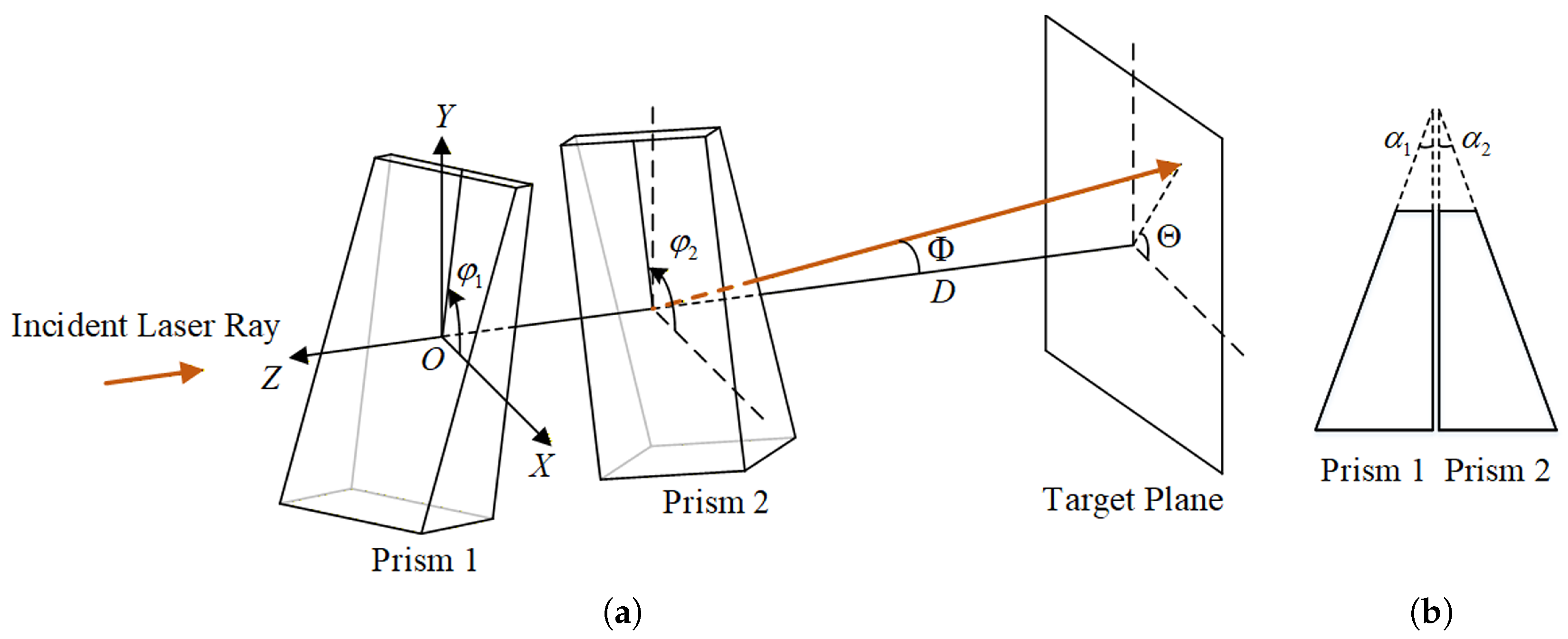
Figure 1 illustrates the beam steering principle of the Risley prism system, alongside its coordinate system and one possible configuration. The system features two refractive prisms rotating independently around a common axis, which concurrently serves as the optical axis. The prism closer to the light source is labeled as Prism 1, while the adjacent prism is labeled as Prism 2. Their respective refractive indices and apex angles are denoted as $n_1$, $n_2$, and ${\alpha }_1$, ${\alpha }_2$, respectively. Rotational angular positions are represented as ${\phi }_1$ and ${\phi }_2$, which are measured from each prism’s thin edge to the positive x-axis, with positive rotations defined toward the positive y-axis within a 2$\pi$ range. The distance between the exit surface of Prism 2 and the target plane is denoted as D. On this plane, the resulting beam position is given by the polar coordinates $(\mathsf{\Phi },\mathsf{\Theta })$, representing deflection and azimuth angles, respectively. Theoretically, full coverage of the accessible deflection range is achieved by appropriately adjusting ${\phi }_1$ and ${\phi }_2$.

Since the Risley prism pair performs target tracking based on a known target motion trajectory, deriving an accurate inverse solution is essential. Therefore, this paper introduces a two-step solution method based on non-paraxial ray tracing theory.

Direction cosines of the beam emerging are given by

$$S^r=(K,L,M)$$

(1)

When the incident beam aligns with the negative z-axis, direction cosines for the resulting emergent ray vector are formulated as

$$\left\{\begin{array}{cc}\hfill K& =d_{1}cos{\phi }_1+d_{3}sin{\alpha }_{2}cos{\phi }_2\hfill \\ \hfill L& =d_{1}sin{\phi }_1+d_{3}sin{\alpha }_{2}sin{\phi }_2\hfill \\ \hfill M& =d_2-d_{3}cos{\alpha }_2\hfill \end{array}\right.$$

(2)

where

$$\left\{\begin{array}{cc}\hfill d_1& ={\displaystyle \frac{n_2}{n_1}}sin{\alpha }_1\left(cos{\alpha }_1-\sqrt{n_1^2-{sin}^2{\alpha }_1}\right)\hfill \\ \hfill d_2& =-{\displaystyle \frac{n_2}{n_1}}\left(\sqrt{n_1^2-{sin}^2{\alpha }_1}cos{\alpha }_1+{sin}^2{\alpha }_1\right)\hfill \\ \hfill d_3& =-\left(d_{1}sin{\alpha }_{2}cos\Delta \phi -d_{2}cos{\alpha }_2\right)\hfill \\ & +\sqrt{1-n_2^2+{\left(d_{1}sin{\alpha }_{2}cos\Delta \phi -d_{2}cos{\alpha }_2\right)}^2}\hfill \\ \hfill \Delta \phi & ={\phi }_2-{\phi }_1\hfill \end{array}\right.$$

Notably, the parameters defined in Equation (2) are only applicable to the prism configuration shown in Figure 1b. For different structural setups, alternative parameter sets are available in [45]. Based on these parameters, the expressions for deflection and azimuth angles are as follows:

$$\mathsf{\Phi }=arccos(-M)$$

(3)

$$\mathsf{\Theta }=\left\{\begin{array}{cccc}\hfill & arctan\left({\displaystyle \frac{L}{K}}\right),\hfill & \hfill & \mathrm{if}K>0\mathrm{and}L\ge 0\hfill \\ \hfill & \hfill & & \mathrm{or}K=0\mathrm{and}L>0\hfill \\ \hfill & arctan\left({\displaystyle \frac{L}{K}}\right)+2\pi ,\hfill & \hfill & \mathrm{if}K\ge 0\mathrm{and}L<0\hfill \\ \hfill & \mathrm{undefined},\hfill & \hfill & \mathrm{if}K=0\mathrm{and}L=0\hfill \\ \hfill & arctan\left({\displaystyle \frac{L}{K}}\right)+\pi ,\hfill & \hfill & \mathrm{otherwise}\hfill \end{array}\right.$$

(4)

Given a target trajectory, deflection and azimuth angles are known. Therefore, the cosine component M is derived from the deflection angle via Equation (3). This value, along with known refractive indices and apex angles, is then used to inversely solve Equation (2), yielding the relative orientation angle $|\Delta \phi |$ between both prisms:

$$|\Delta \phi |=arccos\left({\displaystyle \frac{1}{d_{1}tan{\alpha }_2}}\left\{d_2+{\displaystyle \frac{1}{2(d_2+cos\mathsf{\Phi })}}\left[1-n_2^2-{\left({\displaystyle \frac{d_2+cos\mathsf{\Phi }}{cos{\alpha }_2}}\right)}^2\right]\right\}\right)$$

(5)

Assuming Prism 1 remains stationary at the zero position, Prism 2 rotates forward until their orientation angle reaches $|\Delta \phi |$ (i.e., ${\phi }_1=0$, ${\phi }_2=|\Delta \phi |$). Substituting deflection angular positions of the two prisms into Equation (2) yields cosine components $K_a$ and $L_a$, from which the corresponding beam azimuth angle ${\mathsf{\Theta }}_a$ is obtained via Equation (4). Subsequently, both prisms rotate synchronously through a common angle $\mathsf{\Theta }-{\mathsf{\Theta }}_a$ to steer the emergent beam to the desired azimuth angle $\mathsf{\Theta }$. Consequently, rotational angular positions are determined as follows:

$$\left\{\begin{array}{cc}\hfill {\phi }_1{)}_a& =\mathsf{\Theta }-{\mathsf{\Theta }}_a\hfill \\ \hfill {\phi }_2{)}_a& =\mathsf{\Theta }-{\mathsf{\Theta }}_a+|\Delta \phi |\hfill \end{array}\right.$$

(6)

Alternatively, to derive the second solution branch, Prism 1 remains fixed at zero while Prism 2 rotates backward until their orientation angle reaches $|\Delta \phi |$ (i.e., ${\phi }_1=0$, ${\phi }_2=-|\Delta \phi |$). Reapplying Equation (2) with these updated coordinates generates new cosine components $K_b$ and $L_b$, which subsequently determine the intermediate azimuth angle ${\mathsf{\Theta }}_b$ through Equation (4). Finally, applying a synchronous rotational shift $\mathsf{\Theta }-{\mathsf{\Theta }}_b$ to both prisms aligns the emergent beam with the target azimuth angle $\mathsf{\Theta }$. Consequently, the second set of rotational angular positions is given by

$$\left\{\begin{array}{cc}\hfill {\phi }_1{)}_b& =\mathsf{\Theta }-{\mathsf{\Theta }}_b\hfill \\ \hfill {\phi }_2{)}_b& =\mathsf{\Theta }-{\mathsf{\Theta }}_b-|\Delta \phi |\hfill \end{array}\right.$$

(7)

2.2. Selection of the Inverse Solution for Target Tracking

As indicated by Equations (6) and (7), the inverse problem for target tracking yields two independent analytical solutions. However, controlling singularities at the center or edges of the observation field can induce a critical issue: if only a single solution branch is employed for tracking, the required prism rotation angles or rotation speeds increase sharply, potentially exceeding the motor’s driving capabilities. Notably, while singularities in a small range near the edges of the observation field have minimal impact on practical tracking applications, those in the central region are far more critical and require special attention. Therefore, this paper adopts an optimal solution strategy [46]. This strategy leverages the angular difference characteristics of the two sets of solutions to mitigate severe jumps in the target azimuth angle within the central region, thereby alleviating the driving demands on the prism motors.

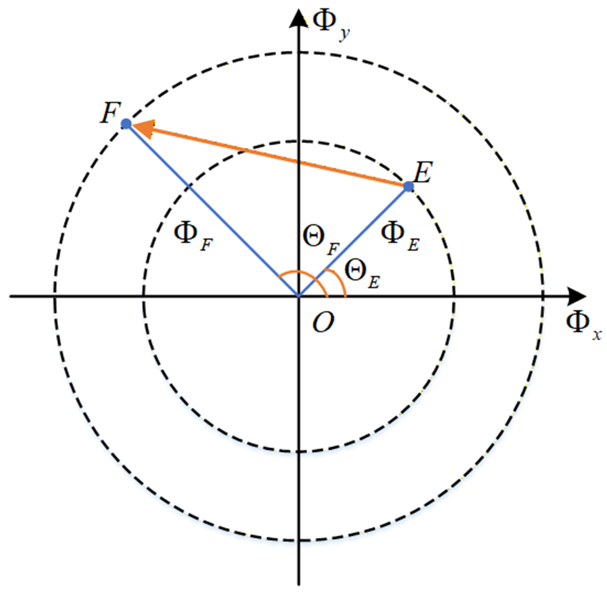
As depicted in Figure 2, assuming the emergent beam tracks a target from point E to point F over a single control period, the corresponding deflection and azimuth angles are denoted as ${\mathsf{\Phi }}_E$, ${\mathsf{\Phi }}_F$, and ${\mathsf{\Theta }}_E$, ${\mathsf{\Theta }}_F$, respectively. Utilizing Equations (5)–(7), two sets of angular position values for the two prisms can be derived. During actual tracking, the initial angular positions of the two prisms at point E can adopt either the first solution set, ${\left({\phi }_{1E}\right)}_a$, ${\left({\phi }_{2E}\right)}_a$, or the second, ${\left({\phi }_{1E}\right)}_b$, ${\left({\phi }_{2E}\right)}_b$. Similarly, the final angular positions at point F can adopt either the first set, ${\left({\phi }_{1F}\right)}_a$, ${\left({\phi }_{2F}\right)}_a$, or the second, ${\left({\phi }_{1F}\right)}_b$, ${\left({\phi }_{2F}\right)}_b$.

During the process of steering the emergent beam from point E to point F, rotation angles required for two prisms are denoted as $|\Delta {\phi }_1|$ and $|\Delta {\phi }_2|$, which represent the differences between the final angular position values corresponding to points F and E. Consequently, two primary scenarios emerge. In the first scenario, the prism system operates within the same solution set. This means if the initial state adopts the first set, the final state remains in the first set:

$$\left\{\begin{array}{cc}\hfill \Delta {\phi }_1& ={\left({\phi }_{1F}\right)}_a-{\left({\phi }_{1E}\right)}_a\hfill \\ \hfill \Delta {\phi }_2& ={\left({\phi }_{2F}\right)}_a-{\left({\phi }_{2E}\right)}_a\hfill \end{array}\right.$$

(8)

Similarly, if the initial state adopts the second set, the final state remains in the second set:

$$\left\{\begin{array}{cc}\hfill \Delta {\phi }_1& ={\left({\phi }_{1F}\right)}_b-{\left({\phi }_{1E}\right)}_b\hfill \\ \hfill \Delta {\phi }_2& ={\left({\phi }_{2F}\right)}_b-{\left({\phi }_{2E}\right)}_b\hfill \end{array}\right.$$

(9)

In the second scenario, the prism system switches between solution sets. Specifically, if the initial state adopts the first set, the final state transitions to the second set:

$$\left\{\begin{array}{cc}\hfill \Delta {\phi }_1& ={\left({\phi }_{1F}\right)}_b-{\left({\phi }_{1E}\right)}_a\hfill \\ \hfill \Delta {\phi }_2& ={\left({\phi }_{2F}\right)}_b-{\left({\phi }_{2E}\right)}_a\hfill \end{array}\right.$$

(10)

Conversely, if the initial state adopts the second set, the final state transitions to the first set:

$$\left\{\begin{array}{cc}\hfill \Delta {\phi }_1& ={\left({\phi }_{1F}\right)}_a-{\left({\phi }_{1E}\right)}_b\hfill \\ \hfill \Delta {\phi }_2& ={\left({\phi }_{2F}\right)}_a-{\left({\phi }_{2E}\right)}_b\hfill \end{array}\right.$$

(11)

According to the optimal solution strategy, if points E and F are situated on the same side of the observation field center (i.e., the azimuth angle difference $|{\mathsf{\Theta }}_F-{\mathsf{\Theta }}_E|$ is less than ${90}^{\circ }$), the same solution set is maintained for tracking. This avoids the sharp increases in prism rotation angles otherwise induced by switching solution sets. Conversely, if points E and F lie on opposite sides of the center (i.e., $|{\mathsf{\Theta }}_F-{\mathsf{\Theta }}_E|$ is between ${90}^{\circ }$ and ${180}^{\circ }$), the required change in the prisms’ angular positions inherently falls between ${90}^{\circ }$ and ${180}^{\circ }$. Under these conditions, switching between solution sets for tracking yields smaller overall rotation angles.

3. Mathematical Model of Instantaneous Power for BLDC Motor

3.1. Mathematical Model of BLDC Motor

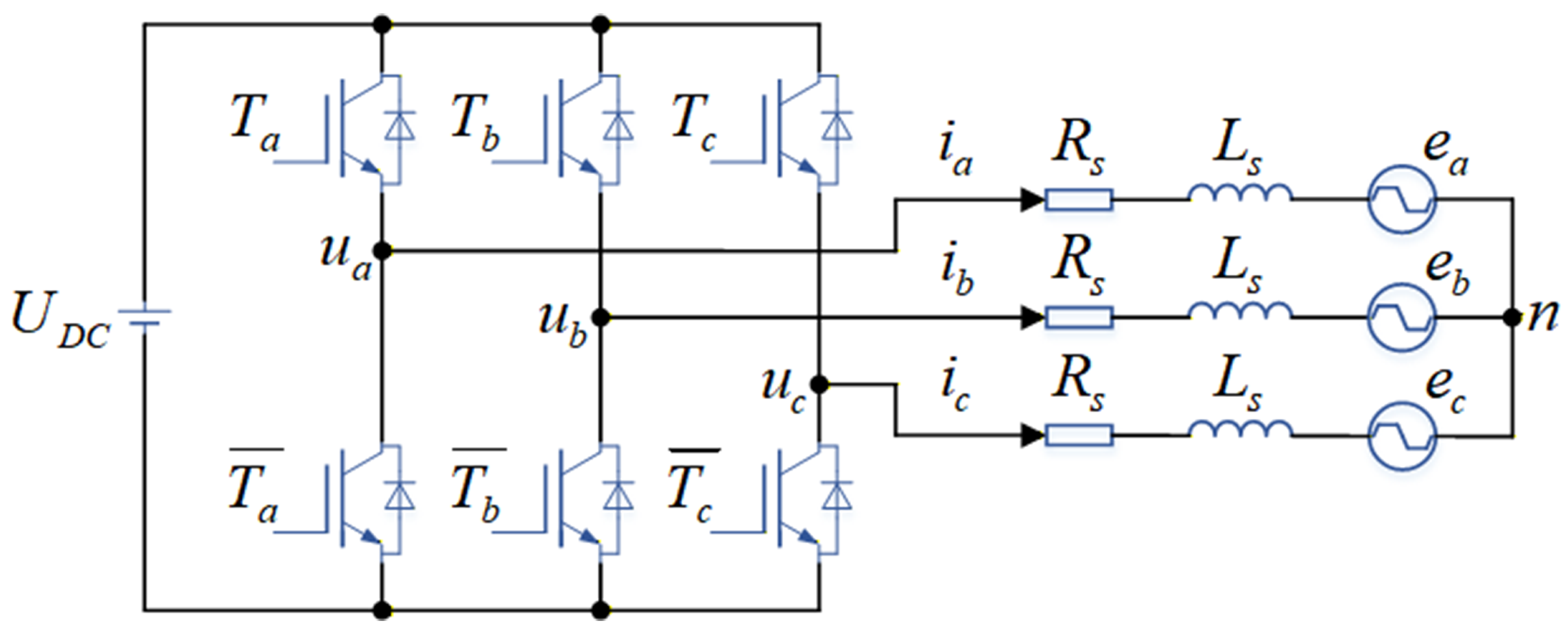
The Risley prism pair primarily employs BLDC motors as core driving components, whose driving characteristics directly determine beam pointing accuracy and stability. Therefore, establishing mathematical models and conducting targeted analyses based on BLDC motor operating principles proves essential. Dynamic models derive from a set of simplifying assumptions. Structurally, rotors utilize surface-mounted permanent magnets, whereas stators feature concentrated, symmetrical star-connected windings. Electromagnetically, both iron losses and magnetic saturation are considered negligible, alongside the fundamental assumption of uniformly distributed permanent magnet flux. Furthermore, torque components such as reluctance and cogging torque are ignored. Under these premises, the simplified equivalent circuit for a two-level, three-phase BLDC motor is presented in Figure 3.

Each stator phase is characterized by phase voltages $u_a$, $u_b$, and $u_c$; nonsinusoidal back EMFs $e_a$, $e_b$, and $e_c$; phase currents $i_a$, $i_b$, and $i_c$; equivalent resistance $R_s$; and equivalent inductance $L_s$. Consequently, stator voltage equations are formulated as follows:

$$\left\{\begin{array}{cc}\hfill u_a& =R_s{i}_a+L_s{\displaystyle \frac{d{i}_a}{dt}}+e_a\hfill \\ \hfill u_b& =R_s{i}_b+L_s{\displaystyle \frac{d{i}_b}{dt}}+e_b\hfill \\ \hfill u_c& =R_s{i}_c+L_s{\displaystyle \frac{d{i}_c}{dt}}+e_c\hfill \end{array}\right.$$

(12)

In Equation (12), back EMFs are expressed as

$$\left\{\begin{array}{cc}\hfill e_a& =N_e{\omega }_m{g}_a\left({\phi }_e\right)\hfill \\ \hfill e_b& =N_e{\omega }_m{g}_b\left({\phi }_e\right)\hfill \\ \hfill e_c& =N_e{\omega }_m{g}_c\left({\phi }_e\right)\hfill \end{array}\right.$$

(13)

where ${\omega }_m$ and ${\phi }_e$ denote mechanical speed and electrical angle of the motor, respectively; $N_e$ represents the back EMF constant; and $g_a\left({\phi }_e\right)$, $g_b\left({\phi }_e\right)$, and $g_c\left({\phi }_e\right)$ indicate unit-level three-phase trapezoidal functions, respectively, formulated as:

$$g_a\left({\phi }_e\right)=\left\{\begin{array}{cccc}\hfill & {\displaystyle \frac{6}{180}}{\phi }_e,\hfill & \hfill & 0^{\circ }<{\phi }_e\le {30}^{\circ }\hfill \\ \hfill & 1,\hfill & \hfill & {30}^{\circ }<{\phi }_e\le {150}^{\circ }\hfill \\ \hfill & -{\displaystyle \frac{6}{180}}{\phi }_e+6,\hfill & \hfill & {150}^{\circ }<{\phi }_e\le {210}^{\circ }\hfill \\ \hfill & -1,\hfill & \hfill & {210}^{\circ }<{\phi }_e\le {330}^{\circ }\hfill \\ \hfill & {\displaystyle \frac{6}{180}}{\phi }_e-12,\hfill & \hfill & {330}^{\circ }<{\phi }_e\le {360}^{\circ }\hfill \end{array}\right.$$

(14)

$$g_b\left({\phi }_e\right)=\left\{\begin{array}{cccc}\hfill & -1,\hfill & \hfill & 0^{\circ }<{\phi }_e\le {90}^{\circ }\hfill \\ \hfill & {\displaystyle \frac{6}{180}}{\phi }_e-4,\hfill & \hfill & {90}^{\circ }<{\phi }_e\le {150}^{\circ }\hfill \\ \hfill & 1,\hfill & \hfill & {150}^{\circ }<{\phi }_e\le {270}^{\circ }\hfill \\ \hfill & -{\displaystyle \frac{6}{180}}{\phi }_e+10,\hfill & \hfill & {270}^{\circ }<{\phi }_e\le {330}^{\circ }\hfill \\ \hfill & -1,\hfill & \hfill & {330}^{\circ }<{\phi }_e\le {360}^{\circ }\hfill \end{array}\right.$$

(15)

$$g_c\left({\phi }_e\right)=\left\{\begin{array}{cccc}\hfill & 1,\hfill & \hfill & 0^{\circ }<{\phi }_e\le {30}^{\circ }\hfill \\ \hfill & -{\displaystyle \frac{6}{180}}{\phi }_e+2,\hfill & \hfill & {30}^{\circ }<{\phi }_e\le {90}^{\circ }\hfill \\ \hfill & -1,\hfill & \hfill & {90}^{\circ }<{\phi }_e\le {210}^{\circ }\hfill \\ \hfill & {\displaystyle \frac{6}{180}}{\phi }_e-8,\hfill & \hfill & {210}^{\circ }<{\phi }_e\le {270}^{\circ }\hfill \\ \hfill & 1,\hfill & \hfill & {270}^{\circ }<{\phi }_e\le {360}^{\circ }\hfill \end{array}\right.$$

(16)

Applying constant power transformations simplifies the aforementioned three-phase model, yielding motor voltage equations within stationary coordinate systems:

$$\left\{\begin{array}{cc}\hfill u_{\alpha }& =R_s{i}_{\alpha }+L_s{\displaystyle \frac{d{i}_{\alpha }}{dt}}+e_{\alpha }\hfill \\ \hfill u_{\beta }& =R_s{i}_{\beta }+L_s{\displaystyle \frac{d{i}_{\beta }}{dt}}+e_{\beta }\hfill \end{array}\right.$$

(17)

where $u_{\alpha }$ and $u_{\beta }$ denote stator voltages; $i_{\alpha }$ and $i_{\beta }$ represent stator currents; and $e_{\alpha }$ and $e_{\beta }$ signify back EMFs. Subscripts $\alpha$ and $\beta$ indicate the stationary axes.

3.2. Analysis of Instantaneous Power

Multiplying both sides of Equation (17) by stator current conjugate $i_{\alpha \beta }^{*}$ to analyze power conservation yields:

$$\left\{\begin{array}{cc}\hfill i_{\alpha }^{*}{u}_{\alpha }& =R_s{\left|i_{\alpha }\right|}^2+L_s{i}_{\alpha }^{*}{\displaystyle \frac{d{i}_{\alpha }}{dt}}+i_{\alpha }^{*}{e}_{\alpha }\hfill \\ \hfill i_{\beta }^{*}{u}_{\beta }& =R_s{\left|i_{\beta }\right|}^2+L_s{i}_{\beta }^{*}{\displaystyle \frac{d{i}_{\beta }}{dt}}+i_{\beta }^{*}{e}_{\beta }\hfill \end{array}\right.$$

(18)

In Equation (18), $i_{\alpha \beta }^{*},u_{\alpha \beta }$ represents total input complex power at the motor port; $R_s{\left|i_{\alpha \beta }\right|}^2$ corresponds to loss on the stator winding; $L_s{i}_{\alpha \beta }^{*}\left(\mathrm{d}{i}_{\alpha \beta }/\mathrm{d}t\right)$ quantifies the power associated with the magnetic energy variation in stator inductance; and $i_{\alpha \beta }^{*}{e}_{\alpha \beta }$ denotes instantaneous total power transferred to the rotor. This rotor-delivered power is written as

$$i_{\alpha \beta }^{*}{e}_{\alpha \beta }=P+jQ$$

(19)

where P and Q correspond to active and reactive power components, respectively, which are given by

$$\left\{\begin{array}{c}\hfill P=i_{\alpha }{e}_{\alpha }+i_{\beta }{e}_{\beta }\\ \hfill Q=i_{\alpha }{e}_{\beta }-i_{\beta }{e}_{\alpha }\end{array}\right.$$

(20)

Mechanically, only the active power component is convertible into useful shaft power. The reactive power component, conversely, is associated with field-weakening operation. To minimize resistive losses and maximize torque-per-ampere ratios, the reactive power is typically regulated to 0 VAr. Consequently, electromagnetic torque is obtained as

$$T_e={\displaystyle \frac{P}{{\omega }_m}}$$

(21)

where ${\omega }_m$ is the mechanical motor speed.

4. Principle of the Proposed Control Method

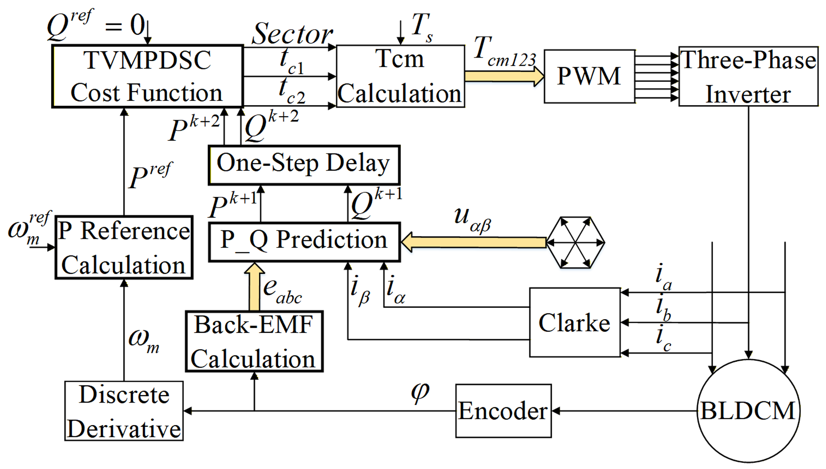
Figure 4 illustrates the control structure of TVMPDSC. This framework primarily comprises a reference power calculation module, a back EMF generation module, an active and reactive power prediction module, a delay compensation module, and a cost function module. The process initiates with the reference power calculation module setting target values for active and reactive powers. Subsequently, the predicted power module utilizes generated back EMFs and measured stator currents to forecast power values. The optimal voltage vector combination and its duration within one control period can be ultimately selected by minimizing the cost function.

4.1. Reference Power

To drive the mechanical load and overcome associated friction and inertia during speed acceleration, the BLDC motor relies on generated electromagnetic torque, which entails the following expression:

$$T_e=T_L+J{\displaystyle \frac{d{\omega }_m}{dt}}+B{\omega }_m$$

(22)

where $T_L$ denotes the mechanical load, whereas J and B represent rotor inertia and viscous friction coefficients, respectively.

Discretizing Equation (22) using the forward Euler method, the mechanical angular velocity at the next discrete time step is

$${\omega }_m^{k+1}={\omega }_m^k+{\displaystyle \frac{T_{sl}}{J}}\left(T_e^k-T_L^k-B{\omega }_m^k\right)$$

(23)

where k indicates the current sampling index, and $T_{sl}$ denotes the mechanical quantity sampling period. Consequently, substituting Equation (21) into Equation (23) calculates active power at the k-th instant:

$$P^k={\omega }_m^k\left[{\displaystyle \frac{J}{T_{sl}}}\left({\omega }_m^{k+1}-{\omega }_m^k\right)+T_L^k+B{\omega }_m^k\right]$$

(24)

Similarly, active power prediction for the $(k+1)$-th step can be obtained as

$$P^{k+1}={\displaystyle \frac{J}{T_{sl}}}{\omega }_m^{k+1}\left({\omega }_m^{k+2}-{\omega }_m^{k+1}\right)+{\omega }_m^{k+1}{T}_L^{k+1}+B{\left({\omega }_m^{k+1}\right)}^2$$

(25)

Following deadbeat control theory, setting ${\omega }_m^{k+2}={\omega }_m^{ref}$ derives the required reference active power:

$$P^{ref}={\displaystyle \frac{J}{T_{sl}}}{\omega }_m^{k+1}\left({\omega }_m^{ref}-{\omega }_m^{k+1}\right)+{\omega }_m^{k+1}{T}_L^{k+1}+B{\left({\omega }_m^{k+1}\right)}^2$$

(26)

Excluding field-weakening operations, the reference value of reactive power $Q^{ref}$ is maintained at 0 VAr.

4.2. Power Prediction

Differentiating active and reactive power expressions within Equation (20) with respect to time yields:

$$\left\{\begin{array}{cc}\hfill {\displaystyle \frac{dP}{dt}}& ={\displaystyle \frac{d{i}_{\alpha }}{dt}}{e}_{\alpha }+i_{\alpha }{\displaystyle \frac{d{e}_{\alpha }}{dt}}+{\displaystyle \frac{d{i}_{\beta }}{dt}}{e}_{\beta }+i_{\beta }{\displaystyle \frac{d{e}_{\beta }}{dt}}\hfill \\ \hfill {\displaystyle \frac{dQ}{dt}}& ={\displaystyle \frac{d{i}_{\alpha }}{dt}}{e}_{\beta }+i_{\alpha }{\displaystyle \frac{d{e}_{\beta }}{dt}}-{\displaystyle \frac{d{i}_{\beta }}{dt}}{e}_{\alpha }-i_{\beta }{\displaystyle \frac{d{e}_{\alpha }}{dt}}\hfill \end{array}\right.$$

(27)

Discretizing Equation (27) using the forward Euler method, active and reactive powers at the $(k+1)$-th step are obtained as

$$\left\{\begin{array}{cc}\hfill P^{k+1}& =-P^k+i_{\alpha }^{k+1}{e}_{\alpha }^k+i_{\alpha }^k{e}_{\alpha }^{k+1}+i_{\beta }^{k+1}{e}_{\beta }^k+i_{\beta }^k{e}_{\beta }^{k+1}\hfill \\ \hfill Q^{k+1}& =-Q^k+i_{\alpha }^{k+1}{e}_{\beta }^k+i_{\alpha }^k{e}_{\beta }^{k+1}-i_{\beta }^{k+1}{e}_{\alpha }^k-i_{\beta }^k{e}_{\alpha }^{k+1}\hfill \end{array}\right.$$

(28)

Given that back EMFs fluctuate at significantly slower rates relative to sampling and switching frequencies, they remain effectively constant throughout the sampling period, formulated as

$$\left\{\begin{array}{cc}\hfill e_{\alpha }^{k+1}& =e_{\alpha }^k\hfill \\ \hfill e_{\beta }^{k+1}& =e_{\beta }^k\hfill \end{array}\right.$$

(29)

Substituting Equation (29) into Equation (28) simplifies $P^{k+1}$ and $Q^{k+1}$ to:

$$\left\{\begin{array}{cc}\hfill P^{k+1}& =i_{\alpha }^{k+1}{e}_{\alpha }^k+i_{\beta }^{k+1}{e}_{\beta }^k\hfill \\ \hfill Q^{k+1}& =i_{\alpha }^{k+1}{e}_{\beta }^k-i_{\beta }^{k+1}{e}_{\alpha }^k\hfill \end{array}\right.$$

(30)

Furthermore, applying forward Euler discretization to Equation (17) obtains stator current vectors for the $(k+1)$-th step:

$$\left\{\begin{array}{cc}\hfill i_{\alpha }^{k+1}& =\left(1-T_s{\displaystyle \frac{R_s}{L_s}}\right)i_{\alpha }^k+{\displaystyle \frac{T_s}{L_s}}\left(u_{\alpha }^k-e_{\alpha }^k\right)\hfill \\ \hfill i_{\beta }^{k+1}& =\left(1-T_s{\displaystyle \frac{R_s}{L_s}}\right)i_{\beta }^k+{\displaystyle \frac{T_s}{L_s}}\left(u_{\beta }^k-e_{\beta }^k\right)\hfill \end{array}\right.$$

(31)

where $T_s$ denotes the electrical sampling period. Because this electrical sampling period is much smaller than the mechanical sampling period, $T_{sl}$ in Equation (23) can be set to $l{T}_s$, where l ranges from 4 to 20.

In summary, given voltage vectors at the k step, Equations (27)–(31) directly compute predicted powers $P^{k+1}$ and $Q^{k+1}$.

4.3. Voltage Vectors Duration

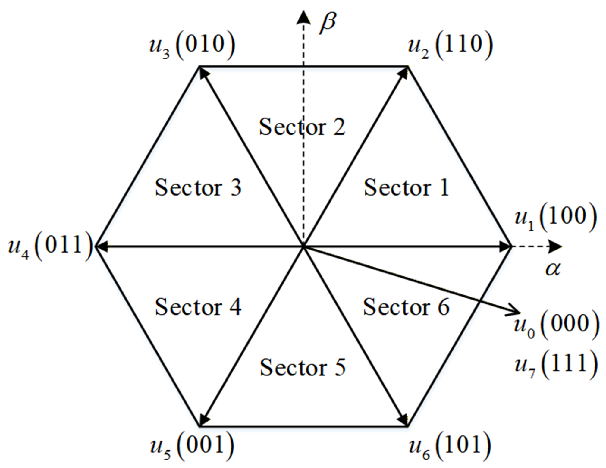
An optimized three-vector-based control scheme is implemented within each control cycle to approximate ideal voltage vectors, effectively suppressing current ripples and boosting overall model predictive direct speed control performance. Rather than acting independently, these three vectors construct a sector-specific composite formulation consisting of two adjacent active voltage vectors alongside a zero vector. Figure 5 depicts the distribution of voltage vectors and voltage sectors for a two-level voltage source inverter (VSI). According to this distribution, operating within the first sector dictates the selection of combination $(u_1,u_2,u_0)$. Similarly, the second sector mandates combination $(u_2,u_3,u_0)$ continuing sequentially. Therefore, the optimization process evaluates a rigidly restricted pool of only six candidate combinations. This constrained set successfully identifies the optimal combination while significantly reducing computational complexity compared to the traditional three-vector strategy.

Given a voltage vector combination $(u_{c1}^k,u_{c2}^k,u_0^k)$ and corresponding durations $t_{c1}^k$, $t_{c2}^k$, $t_0^k$, Equation (31) can be further expressed as

$$\left\{\begin{array}{cc}\hfill i_{\alpha }^{k+1}& ={\displaystyle \frac{1}{L_s}}\left(u_{{\alpha }_{c1}}^k{t}_{c1}^k+u_{{\alpha }_{c2}}^k{t}_{c2}^k\right)+\left(1-T_s{\displaystyle \frac{R_s}{L_s}}\right)i_{\alpha }^k-{\displaystyle \frac{T_s}{L_s}}{e}_{\alpha }^k\hfill \\ \hfill i_{\beta }^{k+1}& ={\displaystyle \frac{1}{L_s}}\left(u_{{\beta }_{c1}}^k{t}_{c1}^k+u_{{\beta }_{c2}}^k{t}_{c2}^k\right)+\left(1-T_s{\displaystyle \frac{R_s}{L_s}}\right)i_{\beta }^k-{\displaystyle \frac{T_s}{L_s}}{e}_{\beta }^k\hfill \end{array}\right.$$

(32)

where $t_{c1}^k+t_{c2}^k+t_0^k=T_s$. Substituting Equation (32) into Equation (30), $P^{k+1}$ and $Q^{k+1}$ are further expressed as

$$\left\{\begin{array}{cc}\hfill P^{k+1}& ={\displaystyle \frac{t_{c1}^k}{L_s}}\left(u_{{\alpha }_{c1}}^k{e}_{\alpha }^k+u_{{\beta }_{c1}}^k{e}_{\beta }^k\right)+\left(1-T_s{\displaystyle \frac{R_s}{L_s}}\right)P^k+{\displaystyle \frac{t_{c2}^k}{L_s}}\left(u_{{\alpha }_{c2}}^k{e}_{\alpha }^k+u_{{\beta }_{c2}}^k{e}_{\beta }^k\right)-{\displaystyle \frac{T_s}{L_s}}{\left|e_{\alpha \beta }^k\right|}^2\hfill \\ \hfill Q^{k+1}& ={\displaystyle \frac{t_{c1}^k}{L_s}}\left(u_{{\alpha }_{c1}}^k{e}_{\beta }^k-u_{{\beta }_{c1}}^k{e}_{\alpha }^k\right)+\left(1-T_s{\displaystyle \frac{R_s}{L_s}}\right)Q^k+{\displaystyle \frac{t_{c2}^k}{L_s}}\left(u_{{\alpha }_{c2}}^k{e}_{\beta }^k-u_{{\beta }_{c2}}^k{e}_{\alpha }^k\right)\hfill \end{array}\right.$$

(33)

Applying tracking conditions $P^{k+1}=P^{ref}$ and $Q^{k+1}=Q^{ref}$, solving Equation (33) yields active vector durations $t_{c1}^k$ and $t_{c2}^k$:

$$\left\{\begin{array}{cc}\hfill t_{c1}^k& ={\displaystyle \frac{F-(L_s-T_s{R}_s)\left(P^k-S_{c2}{Q}^k\right)}{\left(u_{{\alpha }_{c1}}^k+S_{c2}{u}_{{\beta }_{c1}}^k\right)e_{\alpha }^k+\left(u_{{\beta }_{c1}}^k-S_{c2}{u}_{{\alpha }_{c1}}^k\right)e_{\beta }^k}}\hfill \\ \hfill t_{c2}^k& ={\displaystyle \frac{F-(L_s-T_s{R}_s)\left(P^k-S_{c1}{Q}^k\right)}{\left(u_{{\alpha }_{c2}}^k+S_{c1}{u}_{{\beta }_{c2}}^k\right)e_{\alpha }^k+\left(u_{{\beta }_{c2}}^k-S_{c1}{u}_{{\alpha }_{c2}}^k\right)e_{\beta }^k}}\hfill \end{array}\right.$$

(34)

where

$$\left\{\begin{array}{cc}\hfill F& =L_s{P}^{ref}+T_s{\left|e_{\alpha \beta }^k\right|}^2\hfill \\ \hfill S_{c1}& ={\displaystyle \frac{u_{{\alpha }_{c1}}^k{e}_{\alpha }^k+u_{{\beta }_{c1}}^k{e}_{\beta }^k}{u_{{\alpha }_{c1}}^k{e}_{\beta }^k-u_{{\beta }_{c1}}^k{e}_{\alpha }^k}}\hfill \\ \hfill S_{c2}& ={\displaystyle \frac{u_{{\alpha }_{c2}}^k{e}_{\alpha }^k+u_{{\beta }_{c2}}^k{e}_{\beta }^k}{u_{{\alpha }_{c2}}^k{e}_{\beta }^k-u_{{\beta }_{c2}}^k{e}_{\alpha }^k}}\hfill \end{array}\right.$$

Should either $t_{c1}^k$ or $t_{c2}^k$ exceed the control period $T_s$, its value is saturated at $T_s$. Finally, zero vector duration $t_0^k$ is determined by

$$t_0^k=T_s-t_{c1}^k-t_{c2}^k$$

(35)

4.4. Selection of Optimal Vector Combination

After calculating durations for all six candidate combinations, a cost function is required to evaluate their control effectiveness on active and reactive powers, which is defined as

$$Cost={\left(P^{ref}-P^{k+1}\right)}^2+{\left(Q^{ref}-Q^{k+1}\right)}^2$$

(36)

The first and second terms represent active and reactive power prediction errors, respectively. For both terms, a smaller value indicates superior control performance. Consequently, minimizing this cost function identifies the optimal voltage vector combination.

4.5. Delay Compensation

Considering that a digital signal processor inherently requires computation time, the optimal voltage vector cannot be applied immediately after sampling, inducing a one-step delay. Therefore, compensation for the one-step delay is necessary. Firstly, stator current vectors at the $(k+1)$-th step ($i_{\alpha }^{k+1}$ and $i_{\beta }^{k+1}$) are predicted via Equation (31). Subsequently, treating these predictions as initial conditions, Equation (31) is reapplied to derive currents for the $(k+2)$-th step ($i_{\alpha }^{k+2}$ and $i_{\beta }^{k+2}$). Finally, active and reactive powers at the $(k+2)$-th step ($P^{k+2}$ and $Q^{k+2}$) are calculated using Equations (29) and (30). Accordingly, the modified cost function is formulated as

$$Cos{t}^{\prime }={\left(P^{ref}-P^{k+2}\right)}^2+{\left(Q^{ref}-Q^{k+2}\right)}^2$$

(37)

5. Performance Analysis of Speed Control in the Prism Motor System

In order to comprehensively assess the performance of TVMPDSC, comparative simulation experiments are conducted using three control methods: DVMPPC, three-vector-based model predictive power control (TVMPPC), and TVMPDSC. These experiments systematically evaluate steady-state operation, robustness, variable-speed tracking, and real-time feasibility. This experimental framework implements a uniform 50 $\mathsf{\mu }$s control period across all methods. Additionally, both TVMPPC and TVMPDSC employ the seven-segment modulation strategy, which ensures operation at a fixed 20 kHz switching frequency. To rigorously evaluate the three aforementioned control methods under actual hardware constraints, practical measurement noise and quantization errors are introduced into the feedback loops. Specifically, Additive White Gaussian Noise (AWGN) with a 0.05 A standard deviation is injected into phase current measurements to simulate thermal noise and analog-to-digital converter (ADC) inaccuracies. Furthermore, to replicate the discrete physical characteristics of the high-precision optical encoder utilized in the Risley prism pair (1.8 arcsec resolution), a Pseudo-Quantization Noise (PQN) model is adopted. It is implemented by superimposing uniformly distributed random errors onto ideal sensor outputs. Noise amplitudes are strictly confined to their respective quantization limits, featuring a maximum deviation of 4.36 × 10⁻⁶ rad for angular position and 0.166 rpm for rotational speed. This stochastic approach effectively avoids non-physical solver chattering while authentically emulating the hardware noise floor.

It is worth noting that speed-loop PI controllers for both DVMPPC and TVMPPC methods are fully optimized to ensure a strictly fair comparison and address the inherent performance limitations of cascaded structures. Specifically, PI gains (Kp and Ki) are initially tuned using the Ziegler-Nichols heuristic method and subsequently fine-tuned through iterative step-response tests to minimize the Integral of Time-weighted Absolute Error (ITAE). This rigorous tuning process guarantees that they operate at their maximum dynamic and steady-state tracking potential, ensuring that comparative advantages demonstrated by the proposed tuning-free TVMPDSC are fundamentally structural rather than the result of suboptimal parameter selection.

The employed BLDC motor parameters are listed in

Table 1. Key BLDC motor parameters.

Parameter	Value and Unit
Magnetic flux	$0.0118\mathrm{Wb}$
Rated torque	$0.53\mathrm{N}·\mathrm{m}$
Number of poles	8
Rated rotor speed	$2610\mathrm{rpm}$
Back-EMF constant $K_e$	$0.094{\mathrm{V}·\mathrm{rpm}}^{-1}$
Rotational inertial J	$0.001{\mathrm{kg}·\mathrm{m}}^2$
Resistance $R_s$	$0.405\mathsf{\Omega }$
Inductance $L_s$	3.8 × 10−4 H
DC bus voltage $U_{dc}$	$33\mathrm{V}$

.

5.1. Steady-State Performance

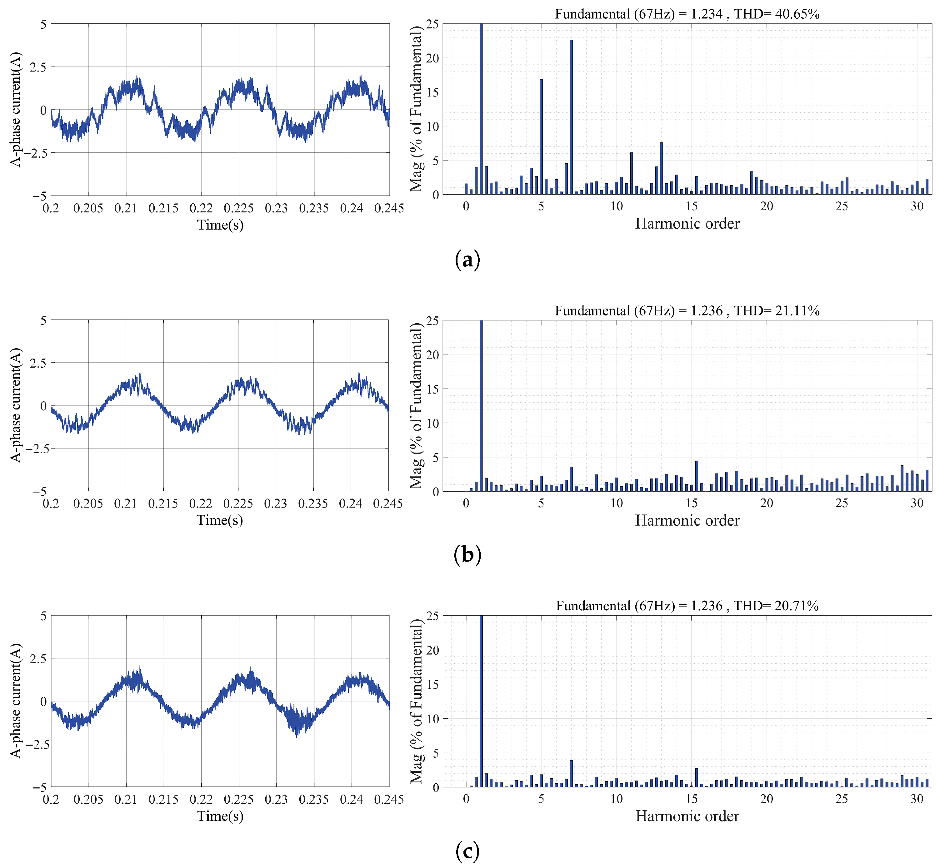
With the motor operating under the conditions of a load torque equivalent to 40% of its rated value and a rotational speed of 500 rpm, Figure 6 illustrates steady-state phase A current waveforms as well as their corresponding total harmonic distortion (THD) metrics across the three distinct control strategies.

As clearly depicted in Figure 6a, DVMPPC exhibits a highly distorted current waveform with a significant THD of 40.65%. Its corresponding FFT spectrum reveals severe low-order harmonic injection, particularly at the 5th and 7th harmonic orders. Such profound distortion stems primarily from limited degrees of freedom inherent to double-vector modulation. When subjected to the injected realistic measurement noise and quantization errors, DVMPPC struggles to synthesize precise voltage vectors necessary for accurate compensation, leading to severe current degradation. Conversely, TVMPPC and TVMPDSC yield notably smoother current waveforms, as demonstrated in Figure 6b,c. By employing three discrete vectors alongside a seven-segment modulation scheme, both TVMPPC and TVMPDSC effectively expand voltage synthesis resolution. This enhanced modulation capability heavily suppresses the prominent 5th and 7th harmonics, drastically reducing THD to 21.11% and 20.71%, respectively, even under the influence of practical hardware noise. Consequently, TVMPDSC completely eliminates the cascaded control structure while successfully preserving excellent underlying electromagnetic modulation quality.

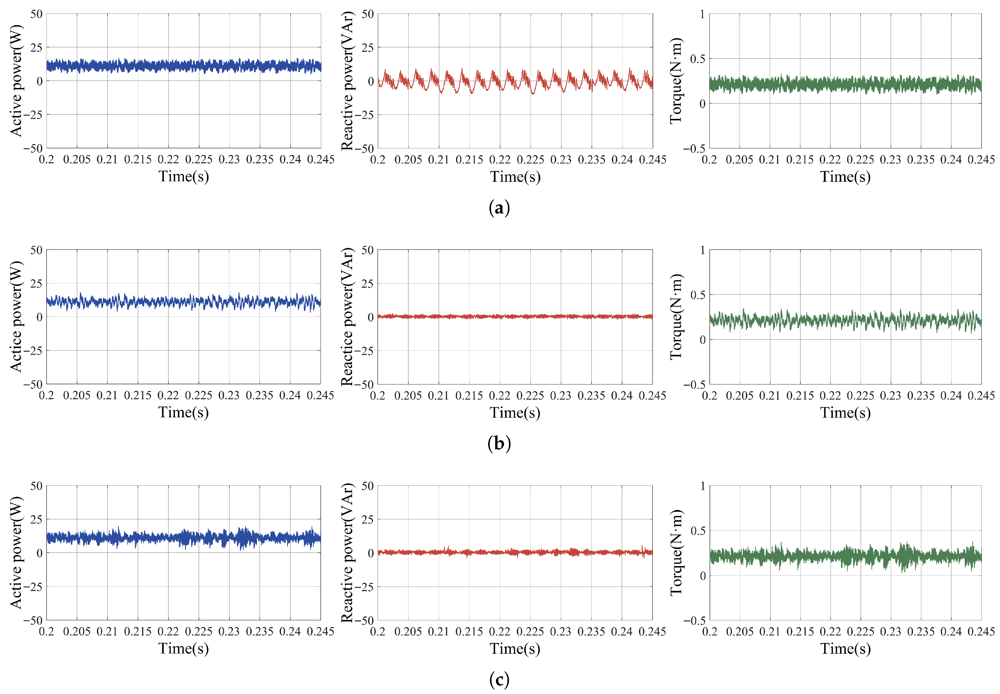
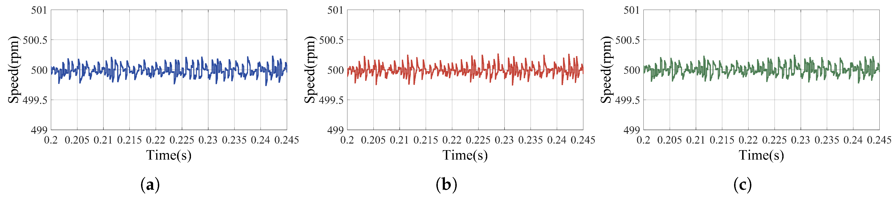
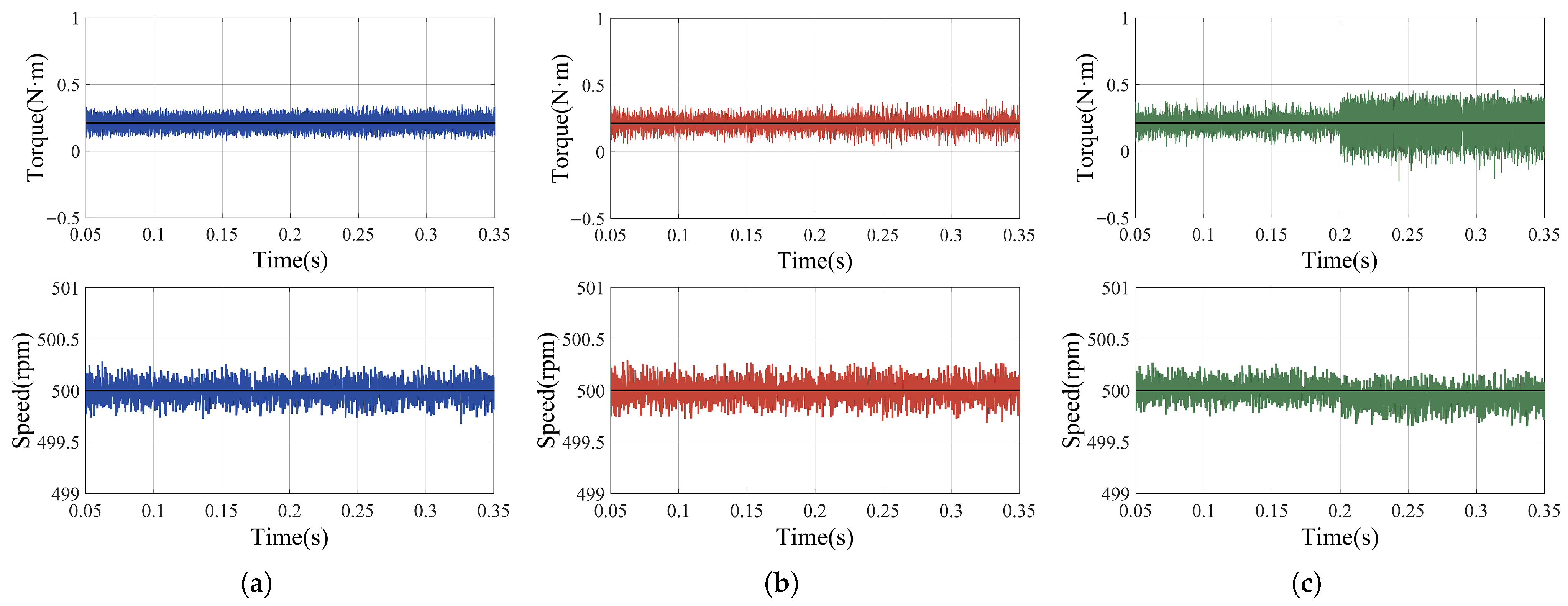
Under identical conditions to Figure 6 and Figure 7, it compares active power, reactive power, and ripple in electromagnetic torque among the three control methods, whereas Figure 8 details fluctuations in rotational speed. For the sake of better facilitating comparison, this paper introduces the torque ripple coefficient to evaluate steady-state torque ripple phenomena, which is explicitly defined as

$${\left(T_e\right)}_{\mathrm{ripple}}={\displaystyle \frac{\sqrt{\frac{1}{n}{\sum }_{i=1}^n{\left[{\left(T_e\right)}_i-{\left(T_e\right)}_{\mathrm{ave}}\right]}^2}}{{\left(T_e\right)}_{\mathrm{ave}}}}\times 100\%$$

(38)

where ${\left(T_e\right)}_i$ and ${\left(T_e\right)}_{\mathrm{ave}}$ represent instantaneous and average electromagnetic torque, respectively. The calculation method for speed ripple coefficient ${\left({\omega }_r\right)}_{\mathrm{ripple}}$ is the same as that for torque ripple coefficient. Regarding steady-state power fluctuation evaluations, active and reactive power performance is characterized by the ensuing set of indicators:

$$\left\{\begin{array}{cc}\hfill \Delta P& =P_{\max }-P_{\min }\hfill \\ \hfill \Delta Q& =Q_{\max }-Q_{\min }\hfill \end{array}\right.$$

(39)

where $P_{\max }$, $P_{\min }$, $Q_{\max }$, and $Q_{\min }$ are denote maximum and minimum respective power components. All steady-state performance metrics are summarized in

Table 2. Steady-state performance comparison of different control methods.

Method	Current THD (%)	$\mathsf{\Delta }\mathit{P}$ (W)	$\mathsf{\Delta }\mathit{Q}$ (VAr)	${\left({\mathit{T}}_{\mathit{e}}\right)}_{\mathbf{ripple}}$ (%)	${\left({\mathit{\omega }}_{\mathit{r}}\right)}_{\mathbf{ripple}}$ (%)
DVMPPC	40.65	12.27	19.58	17.75	0.0183
TVMPPC	21.11	14.53	4.30	19.06	0.0170
TVMPDSC	20.71	18.07	9.53	18.43	0.0172

.

As illustrated in Figure 7 and Table 2, DVMPPC exhibits inferior performance in reactive power regulation. Its steady-state reactive power fluctuation reaches up to 19.58 VAr, manifested by severe waveform oscillations in Figure 7a. This is primarily because dual-vector modulation restricts degrees of freedom in voltage vector synthesis per control period, failing to provide fine voltage resolution necessary to reject high-frequency noise disturbances. In contrast, TVMPPC and TVMPDSC strategies, which employ three-vector modulation, significantly suppress reactive power fluctuations to 4.30 VAr and 9.53 VAr, respectively (as depicted in Figure 7b,c). These findings clearly demonstrate that integrating three-vector optimization and a seven-segment modulation strategy can drastically enhance the tracking accuracy of the stator flux linkage trajectory, thereby effectively mitigating redundant excitation energy losses that do not contribute to mechanical torque.

However, there is a counterintuitive phenomenon: active power fluctuation of 12.27 W and torque ripple of 17.75% under DVMPPC are actually slightly lower than 14.53 W and 19.06% yielded by advanced TVMPPC strategy. This observation does not imply superiority of DVMPPC; rather, it is dictated by inherent trapezoidal back EMF characteristics of BLDC motors. The current waveform produced by DVMPPC is highly distorted, with a total harmonic distortion reaching 40.65%. When this non-sinusoidal current, rich in low-order harmonics, interacts with the trapezoidal back EMF profile, it coincidentally mitigates electromagnetic torque ripple to some extent. Nevertheless, this marginal advantage in torque ripple comes at the severe cost of degraded stator current quality and significant harmonic heating in the motor. In contrast, TVMPPC and TVMPDSC substantially improve sinusoidal quality of currents, reducing THD to approximately 20%. The coupling of highly sinusoidal currents with trapezoidal back EMF naturally excites slightly higher torque ripples. This represents an inevitable physical trade-off that must be accepted when prioritizing superior current quality and minimized harmonic losses. The active power fluctuation of TVMPDSC, recorded at 18.07 W, is higher than the 14.53 W observed in TVMPPC. As depicted in Figure 7c, the active power waveform of TVMPDSC exhibits more noticeable high-frequency spikes. This discrepancy arises because TVMPPC relies on the integral term of the PI controller to artificially smooth out quantization steps introduced by the 1.8-arcsec encoder. Conversely, TVMPDSC directly calculates reference power using an algebraic dynamic equation. Consequently, its reference active power faithfully reflects actual mechanical quantization steps and velocity measurement noise, inevitably leading to frequent fine-tuning of the active power tracking target.

As illustrated in Figure 8, steady-state speed waveforms across all three control algorithms exhibit high consistency. Their speed ripple coefficients converge closely to 0.0183%, 0.0170%, and 0.0172%, respectively. Specifically, the integral term of the outer-loop PI controller in TVMPPC effectively smooths out discrete speed measurement steps caused by the 1.8-arcsec encoder, providing an exceptionally smooth reference power signal for the inner loop. Coupled with high-precision three-vector modulation, its torque ripples are predominantly concentrated in high-frequency bands. These high-frequency ripples are easily and completely filtered out by the rotor’s mechanical inertia, resulting in the lowest speed fluctuation. In contrast, due to the poor voltage synthesis precision of the dual-vector strategy under noise interference, DVMPPC excites numerous low-order current harmonics that translate into low-frequency torque ripples. Although the rotor’s mechanical inertia inherently acts as a natural low-pass filter, it struggles to fully eliminate these large-amplitude, low-frequency electromagnetic disturbances, ultimately leading to a slight increase in mechanical speed ripple. TVMPDSC entirely eliminates the outer-loop PI controller, directly calculating reference active power via dynamic equations based on actual speed containing quantization noise. While this causes its reference active power to exhibit more macroscopic high-frequency fluctuations, TVMPDSC leverages exceptional single-period execution precision of three-vector optimization and seven-segment modulation strategies to achieve instantaneous and deadbeat tracking of these minute power-fluctuation commands. This high-frequency and instantaneous fine-tuning of electromagnetic power establishes a perfect dynamic balance with the inherent mechanical inertia of the rotor. Finally, TVMPDSC effectively utilizes physical inertial damping of the system itself to yield a mechanical speed fluctuation that is virtually identical to that of TVMPPC.

Steady-state experimental results demonstrate that TVMPDSC maintains outstanding speed stability despite introduced measurement noise and quantization errors.

5.2. Robust Performance

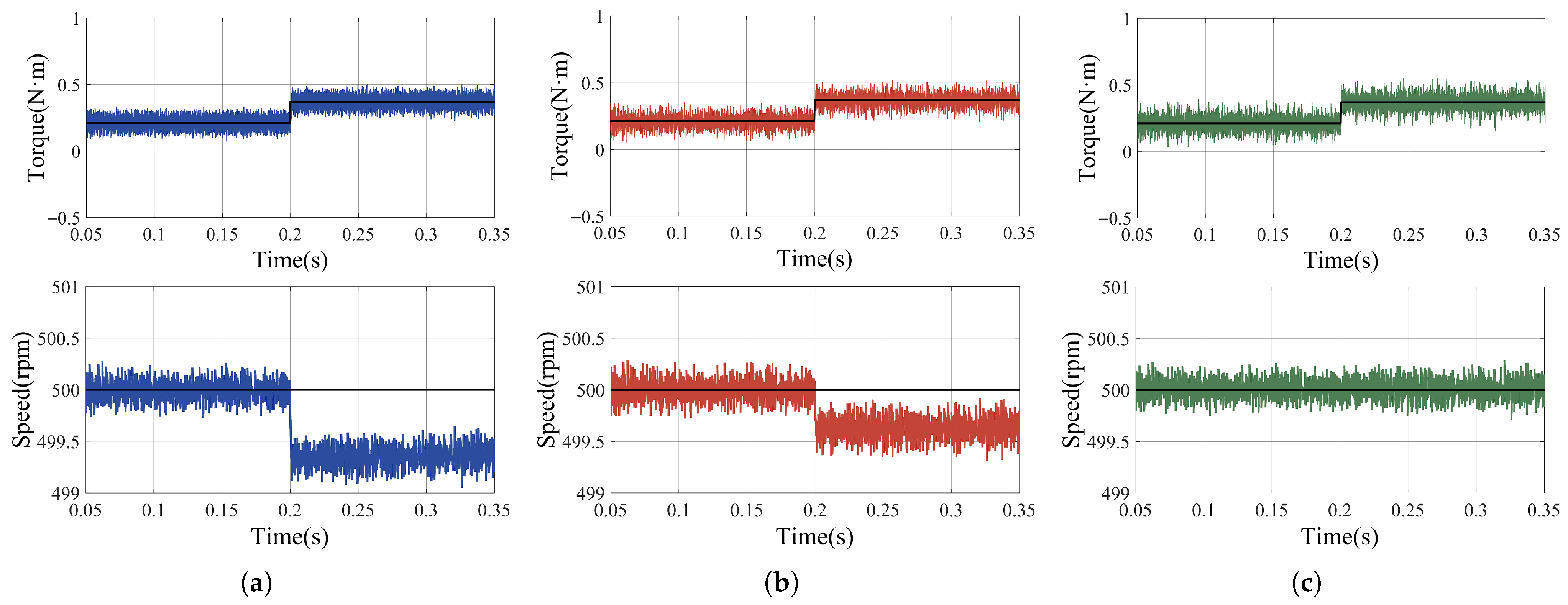
To further validate the robustness of the proposed TVMPDSC against parameter uncertainties and external disturbances, a series of evaluations is conducted under the same baseline conditions employed in the steady-state analysis. These include comparative tests on electrical parameter mismatches and sudden external load impacts across the three control methods, as well as a dedicated assessment of mechanical parameter mismatches specifically for TVMPDSC. Figure 9 illustrates the variations in electromagnetic torque and speed waveforms under the three control methods when a 30% increase in the stator inductance parameter is introduced into the controller at 0.2 s. As observed in Figure 9, the torque and speed ripples of the DVMPPC remain almost unchanged. Notably, TVMPPC exhibits exceptionally strong disturbance rejection against inductance variations, with virtually no observable fluctuations in its torque and speed ripples. In contrast, TVMPDSC experiences a noticeable increase in the amplitude of its torque ripples, accompanied by a slight deviation in the average torque. Correspondingly, the speed ripple amplitude increases slightly, and the average speed drops by approximately 0.1 rpm. When an inductance parameter mismatch occurs in the system, the modulation precision of DVMPPC is inherently so low that its intrinsic high-frequency harmonics mask effects induced by the parameter mismatch. In TVMPPC, the cascaded PI controller acts as a highly effective low-pass filter to eliminate high-frequency electromagnetic interference signals caused by the parameter mismatch, thereby maintaining the smoothness and stability of the reference active power. Furthermore, its integral action continuously accumulates the speed error, forcefully elevating the reference power command until the average speed precisely recovers to 500 rpm. Conversely, lacking PI filtering and integral compensation mechanisms, TVMPDSC is highly sensitive to high-frequency noise. Upon a parameter mismatch, internal predictive models deviate from actual motor dynamics. Consequently, calculated voltage vector durations lose their optimality, which degrades switching precision and excites more high-frequency current harmonics. Macroscopically, this manifests as a significant increase in the amplitude of electromagnetic torque ripples. Meanwhile, in the absence of an integral term to compensate for unmodeled active power deficits, the system naturally settles at a new physical equilibrium, directly observable as an approximate 0.1-rpm speed deviation. Nevertheless, considering this 0.1-rpm offset represents merely a 0.02% steady-state error relative to a 500-rpm baseline, such performance degradation is virtually negligible. This fully demonstrates that TVMPDSC maintains robust stability and highly acceptable precision against severe electrical parameter uncertainties.

Figure 10 illustrates electromagnetic torque and speed waveform variations for three control methods when a sudden 30% rated load is applied at 0.2 s. As observed in Figure 10, following load impact, electromagnetic torque across all methods increases to balance load demand, yet speed waveforms exhibit distinctly different characteristics. Specifically, average speeds of DVMPPC and TVMPPC drop by 0.7 rpm and 0.4 rpm, respectively. This demonstrates sluggish disturbance rejection, showing no obvious recovery trend within a subsequent 0.15 s observation window. This severe transient degradation stems from a fundamental bandwidth trade-off inherent in cascaded PI controllers. To prevent amplifying high-frequency quantization noise from the 1.8-arcsec encoder and maintain previously demonstrated steady-state smoothness, PI parameters must be tuned conservatively with a low cut-off frequency. Consequently, integral response becomes too sluggish to rapidly accumulate sufficient error for compensating for sudden load impacts. In stark contrast, TVMPDSC exhibits exceptional dynamic stiffness. By omitting PI controllers, TVMPDSC directly calculates required active power via algebraic dynamic equation. Discrete difference terms within this equation inherently possess ultra-high proportional gains, inversely proportional to minute sampling periods. Therefore, this method responds instantaneously to microscopic speed deviations. Through dynamic electromagnetic torque regulation, new load demand is perfectly matched within a single control cycle. Macroscopic transient speed drop is virtually eliminated, leaving only a negligible average speed deviation (under 0.1 rpm) to balance unmodeled load requirements. This result explicitly confirms that TVMPDSC completely bypasses traditional PI control bandwidth limitations, achieving near-instantaneous load disturbance rejection without sacrificing steady-state smoothness.

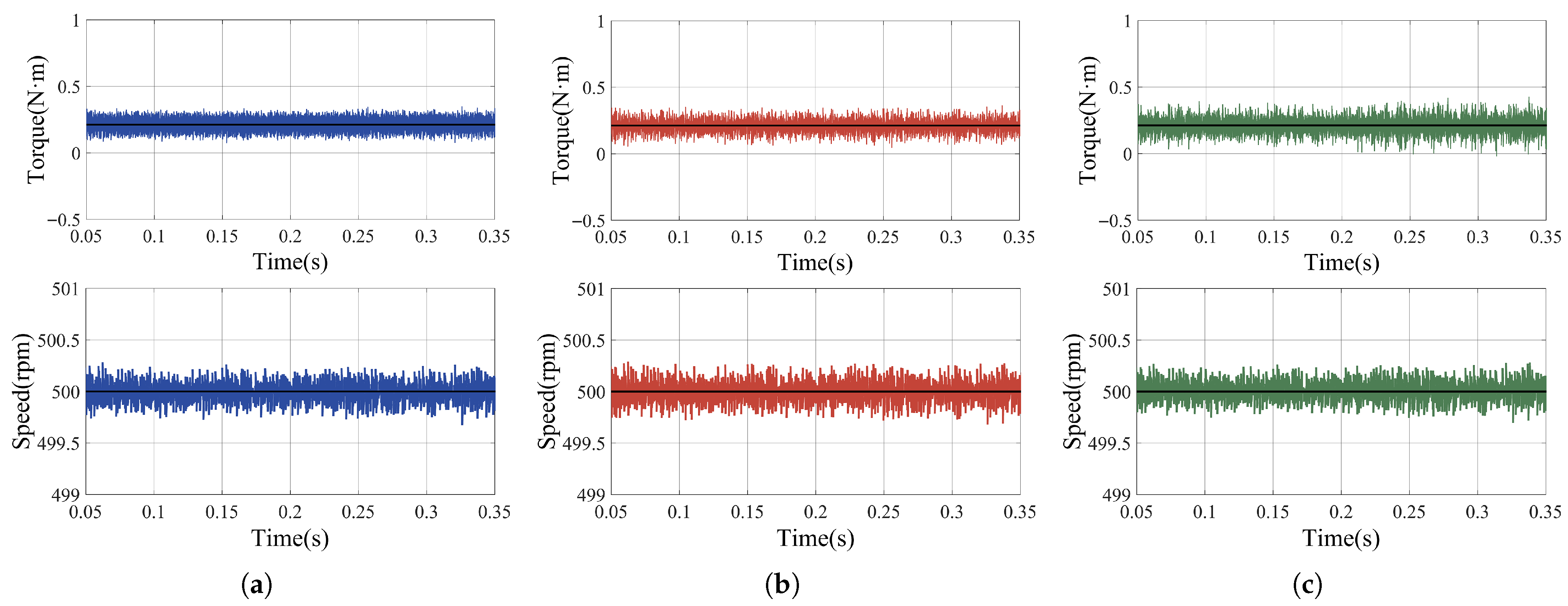
Figure 11 illustrates electromagnetic torque and speed waveform variations under three control methods when the controller’s internal moment of inertia increases by 30% at 0.2 s. As observed, torque and speed ripples for DVMPPC and TVMPPC remain completely stable. This occurs because their outer-loop speed regulation employs PI controllers, rendering algorithm execution entirely independent of rotational inertia. In contrast, TVMPDSC exhibits a noticeable amplitude increase in high-frequency electromagnetic torque ripple, alongside a slight rise in speed ripple amplitude. Such a phenomenon is fundamentally linked to algebraic structures of direct power calculation. TVMPDSC calculates reference active power by explicitly embedding rotational inertia into the dynamic equation. Due to inherent quantization noise from the 1.8-arcsec encoder, the speed feedback signal inevitably exhibits microscopic high-frequency jumps. When controller internal inertia increases by 30%, this inherent noise is additionally amplified by 30% during reference power computation. Transmitted directly to the inner control loop, such an amplified high-frequency command triggers aggressive voltage vector switching. Macroscopically, this manifests as a significant amplitude increase in high-frequency electromagnetic torque ripple. Consequently, intensified torque oscillation naturally causes a slight expansion in mechanical speed ripple amplitude. Although noise is amplified, the system experiences neither control failure nor low-frequency resonance. Actual rotor physical inertia successfully dampens most artificially induced high-frequency torque ripples, ensuring average speed remains completely stable at 500 rpm with zero steady-state offset. Ultimately, these results demonstrate that the proposed TVMPDSC possesses adequate disturbance rejection capability against mechanical parameter uncertainties.

Notably, robustness evaluations for TVMPDSC under stator resistance and viscous friction coefficient mismatches are omitted. Physically, at 500 rpm operating speed, EMF heavily dominates stator voltage equations, rendering resistive voltage drops practically negligible. Therefore, compared with stator inductance, stator resistance variations exert minimal impact on MPPC inner-loop prediction accuracy. Similarly, friction torque governed by viscous friction coefficients constitutes merely a marginal fraction of total mechanical loads. Associated parameter mismatches induce solely microscopic steady-state power deviations, completely masked by inherent quantization noise and external load uncertainties. Consequently, validating system robustness against stator inductance variations, mechanical inertia mismatches, and sudden load impacts possesses high representativeness, proving entirely sufficient for rigorously assessing actual reliability of TVMPDSC.

5.3. Variable Speed Tracking Performance

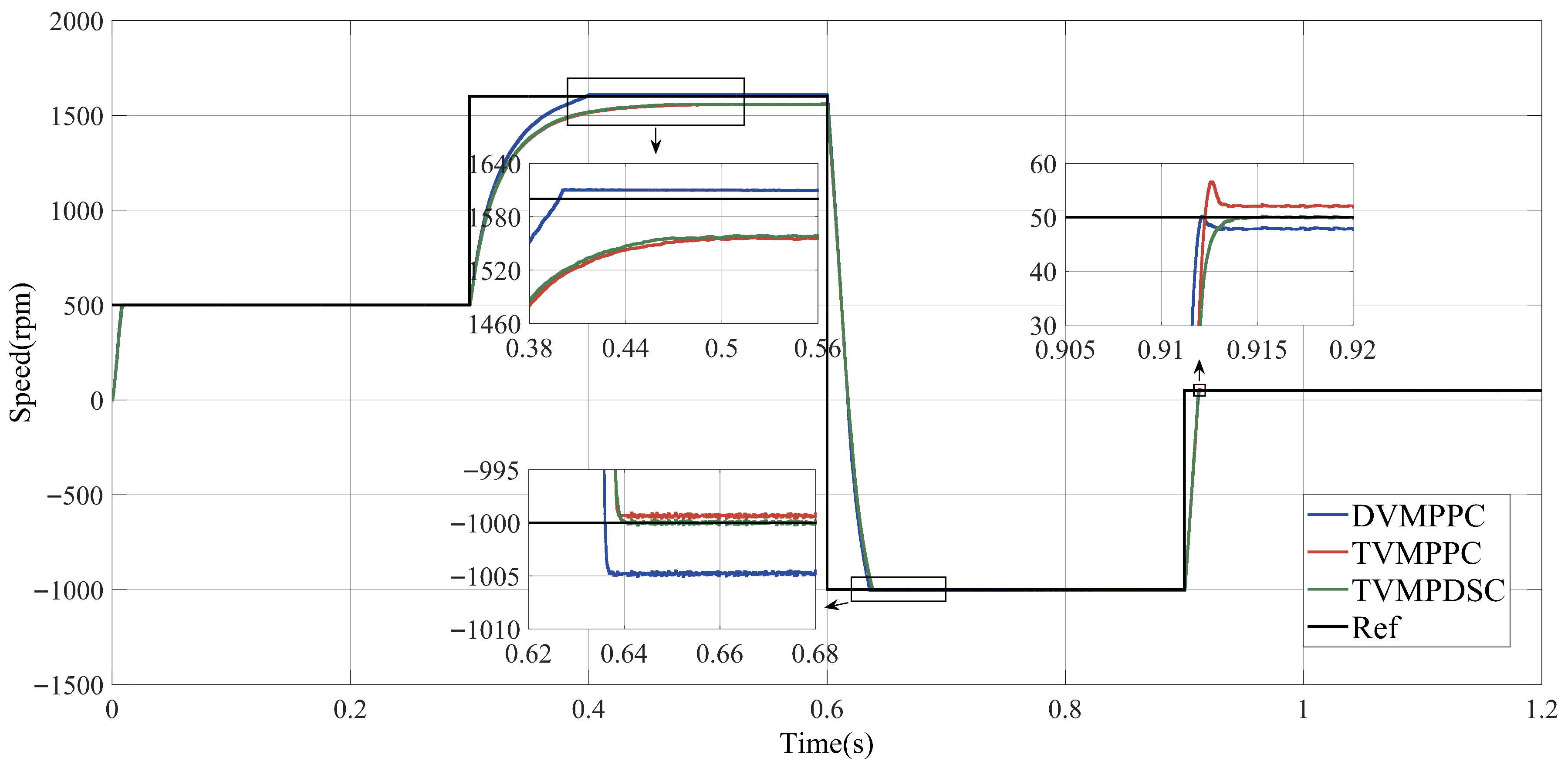
To demonstrate the wide-speed control performance of the proposed TVMPDSC, a comparative variable-speed tracking experiment is conducted. Building upon steady-state experimental conditions, reference speeds are sequentially altered: stepping forward to 1600 rpm at 0.3 s, reversing to −1000 rpm at 0.6 s, and finally recovering to 50 rpm at 0.9 s. Figure 12 illustrates tracking results for three control methods under varying reference speeds.

As Figure 12 illustrates, upon a reference speed step from 500 rpm to 1600 rpm, EMF becomes exceedingly high. Required driving voltage approaches or even exceeds the inverter linear modulation limits. Three-vector optimization and seven-segment modulation strategies of TVMPPC and TVMPDSC must strictly allocate time among two non-zero adjacent vectors and one zero vector within a single control period. To guarantee such high-precision synthesis, synthesized voltage vectors must remain confined within a regular hexagon, typically inside its inscribed circle. Upon voltage margin depletion, three-vector algorithms cannot output greater voltages while maintaining switching rules, thus experiencing premature saturation around 1560 rpm. Double-vector modulation in DVMPPC permits selecting only two active vectors per cycle, with combined durations spanning the entire control period. This enables synthesized voltage vectors to align directly with hexagonal voltage boundaries, thereby generating higher maximum average voltages than voltage vectors of the inscribed circle. However, such an operation essentially enters overmodulation regions, sacrificing current quality to achieve higher ultimate rotational speeds. Upon reference speed stepping from 1600 rpm to −1000 rpm, cascaded methods suffer severe parameter mismatch since PI controllers are tuned exclusively at 500 rpm. Due to inherent modulation degree-of-freedom limitations in double-vector approaches, coarse inner-loop execution precision of DVMPPC amplifies outer-loop PI mismatch errors, generating maximum average speed deviations during steady state. Relying on ultra-high three-vector execution precision, TVMPPC accurately tracks such suboptimal commands, thus yielding a smaller average speed deviation. Conversely, free from PI controller parameter mismatch constraints and combined with high-precision three-vector modulation, TVMPDSC achieves practically zero average speed deviation. Upon a reference speed step from −1000 rpm to 50 rpm, severe integral windup within the PI controller triggers significant overshoot in TVMPPC. Conversely, DVMPPC exhibits obvious undershoot due to restricted voltage synthesis freedom and insufficient resolution at low speeds. Relying on deadbeat calculation and three-vector high-frequency fine-tuning, TVMPDSC instantaneously accomplishes zero-overshoot convergence under physical damping. Experimental results indicate that within reasonable linear physical bandwidths, TVMPDSC achieves wide-speed dynamic adaptability featuring near-zero steady-state errors and no overshoot, representing dynamic performance fundamentally unachievable by both aforementioned control methods.

5.4. Computational Complexity and Real-Time Feasibility

To quantitatively assess processing requirements and real-time feasibility, computational complexity across three control algorithms is analyzed. In model predictive control, computational burden primarily depends on candidate voltage vectors evaluated within cost functions per control period. Theoretical floating-point operations (FLOPs) required per execution cycle for each algorithm are rigorously calculated.

Table 3. Computational complexity of different control methods.

Method	Modulated Vectors	FLOPs per Control Cycle
DVMPPC	2	1872
TVMPPC	3	1427
TVMPDSC	3	1452

summarizes comparative results.

As demonstrated in the evaluation, DVMPPC inherently requires substantial computational effort (1872 FLOPs) stemming from exhaustive global vector space evaluations to determine optimal duty cycles. In contrast, despite synthesizing three voltage vectors, TVMPDSC exhibits a significantly lower computational burden (1452 FLOPs). This efficiency improvement originates from implemented sector-based optimization. By identifying the reference sector first, TVMPDSC strictly confines optimal vector selection to merely six candidate combinations, effectively circumventing exponential computational complexity growth typically associated with multi-vector MPC. Furthermore, compared to TVMPPC (1427 FLOPs), TVMPDSC only introduces a marginal increase of 25 FLOPs. Such a minor addition corresponds entirely to the substitution of the outer-loop PI controller with an algebraic dynamic equation for direct reference power calculation. Consequently, the proposed architecture significantly enhances dynamic tracking stiffness without imposing noticeable computational penalties.

Regarding processing requirements, TVMPDSC involves extensive algebraic floating-point calculations and matrix operations for power prediction and cost function evaluation. Therefore, preventing computational overflow and execution delays necessitates high-performance 32-bit floating-point Digital Signal Processors (DSPs) as foundational hardware.

To validate real-time feasibility, drive control of the Risley prism pair is targeted for physical implementation on a TI TMS320F28379D microcontroller. Operating at a system clock frequency of 200 MHz and equipped with a dedicated hardware Floating-Point Unit (FPU), this processor handles single-precision floating-point calculations at an exceptionally high throughput rate. The theoretical execution time $T_{exec}$ can be mathematically estimated using the following equation:

$$T_{exec}\approx {\displaystyle \frac{N_{FLOPs}\times CPI}{f_{sys}}}$$

(40)

where $N_{FLOPs}$ represents total floating-point operations per cycle; $CPI$ denotes average clock cycles per instruction; and $f_{sys}$ indicates system clock frequency, while the FPU can execute theoretical mathematical instructions with $CPI$ approaching 1, practical implementations incur additional overhead from memory access, pipeline stalling, and conditional branching logic. Therefore, a conservative average $CPI$ ranging from 1.5 to 2.0 is typically assumed. Processing the required 1452 FLOPs on this TI TMS320F28379D microcontroller translates to an estimated theoretical execution time of approximately 10.89 $\mathsf{\mu }$s to 14.52 $\mathsf{\mu }$s.

Given that the fundamental control period of the system is strictly set to 50 $\mathsf{\mu }$s, the worst-case execution time of TVMPDSC occupies less than 30% of the available period. This leaves a robust safety margin of over 35 $\mathsf{\mu }$s for analog-to-digital sampling, high-precision encoder reading, and other background system tasks. Therefore, the proposed TVMPDSC algorithm is highly feasible for real-time implementation, guaranteeing deterministic execution without computational overrun risks in practical applications.

6. Target Tracking Simulation and Analysis

To further validate the effectiveness of TVMPDSC in target-tracking applications, this paper establishes a simulation platform for target tracking with a Risley prism pair and compares the tracking accuracy and stability of the three aforementioned control methods for dynamic targets.

6.1. Control System

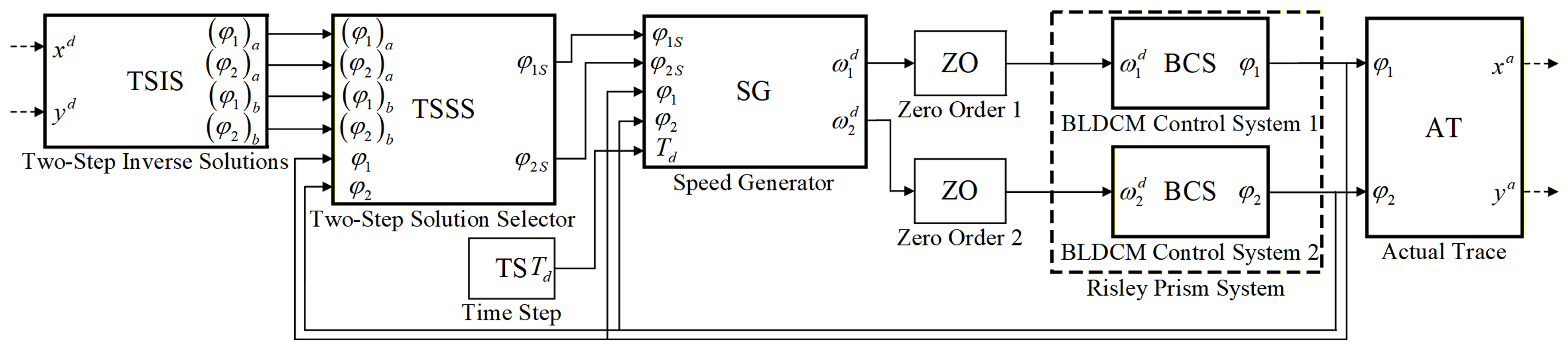
Figure 13 illustrates the control system for target tracking, which mainly consists of a two-step inverse solution solver (TSIS), a two-step inverse solution selector (TSSS), a reference speed generator (SG), a pair of BLDC motor control systems (BCSs), and an actual trajectory output module (AT). The entire control process is described as follows:

Given a reference trajectory and sampling point coordinates $(x^d,y^d)$ on it at each time step $T_d$, the TSIS module generates desired pitch and azimuth angles $({\mathsf{\Phi }}^d,{\mathsf{\Theta }}^d)$ through the following formulas:

$${\mathsf{\Phi }}^d=arctan\left({\displaystyle \frac{\sqrt{{\left(x^d\right)}^2+{\left(y^d\right)}^2}}{D}}\right)$$

(41)

$${\mathsf{\Theta }}^d=\left\{\begin{array}{cccc}\hfill & arctan\left({\displaystyle \frac{y^d}{x^d}}\right),\hfill & \hfill & \mathrm{if}{x}^d>0\mathrm{and}{y}^d\ge 0\hfill \\ \hfill & \hfill & & \mathrm{or}{x}^d=0\mathrm{and}{y}^d>0\hfill \\ \hfill & arctan\left({\displaystyle \frac{y^d}{x^d}}\right)+2\pi ,\hfill & \hfill & \mathrm{if}{x}^d\ge 0\mathrm{and}{y}^d<0\hfill \\ \hfill & \mathrm{undefined},\hfill & \hfill & \mathrm{if}{x}^d=0\mathrm{and}{y}^d=0\hfill \\ \hfill & arctan\left({\displaystyle \frac{y^d}{x^d}}\right)+\pi ,\hfill & \hfill & \mathrm{otherwise}\hfill \end{array}\right.$$

(42)

Subsequently, the module continues to calculate two sets of angular position values using Equations (5)–(7). Evaluating current prism motor positions, the TSSS module outputs the optimal position set yielding minimum angular error. Next, the SG module solves for the desired rotational speeds by differentiating the desired and current angular positions over the time step $T_d$ and holds them at zero order for the same step duration. It is noteworthy that the rotational speeds can be considered constant because the time step is usually set very small. Ultimately, the control systems drive the BLDC motors to achieve target speeds, thereby enabling reference trajectory tracking. The actual trajectory can be reversely derived by the AT module using Equations (1)–(4) and Equations (41) and (42).

6.2. Results and Analysis of Target Tracking

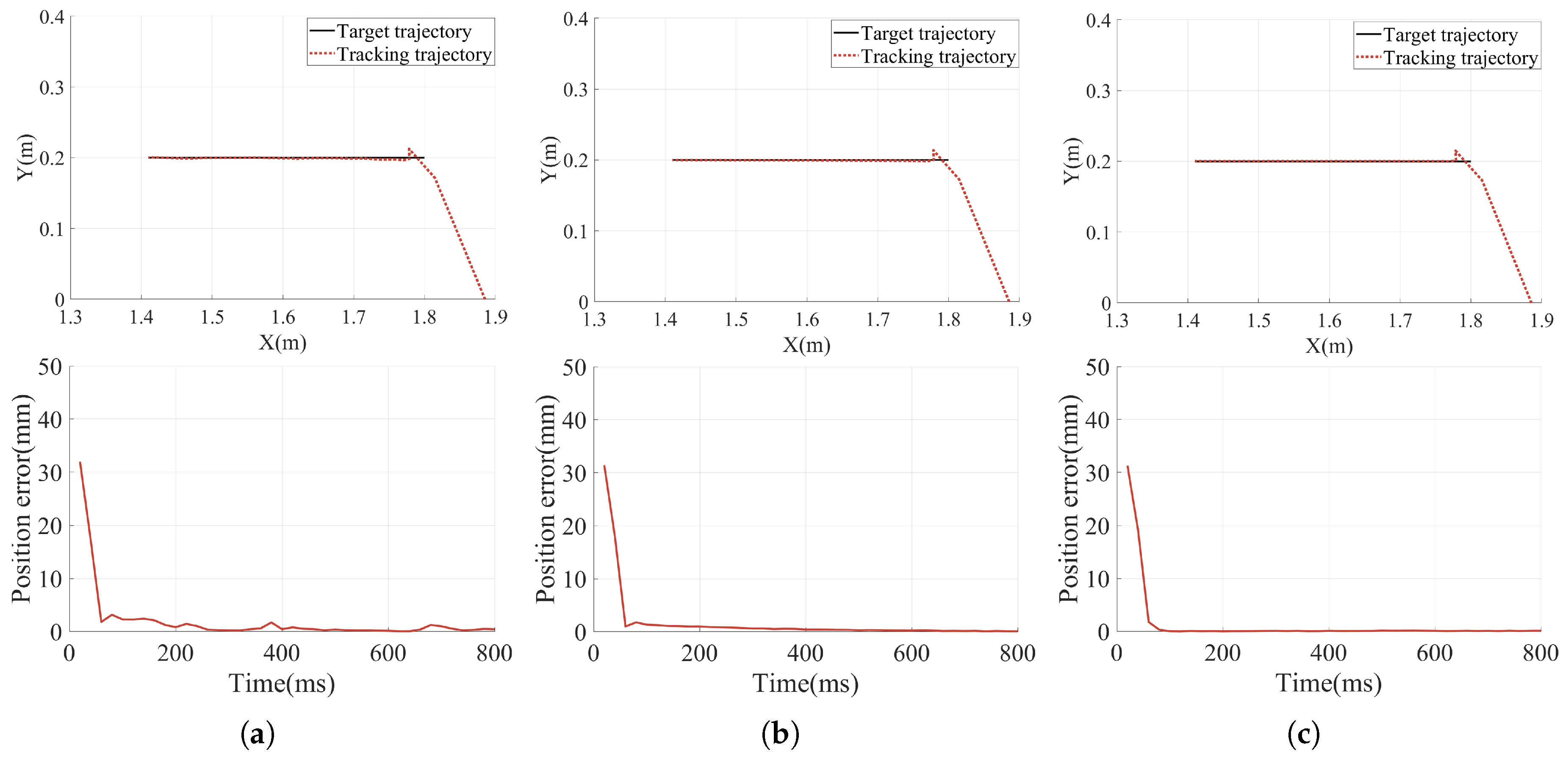
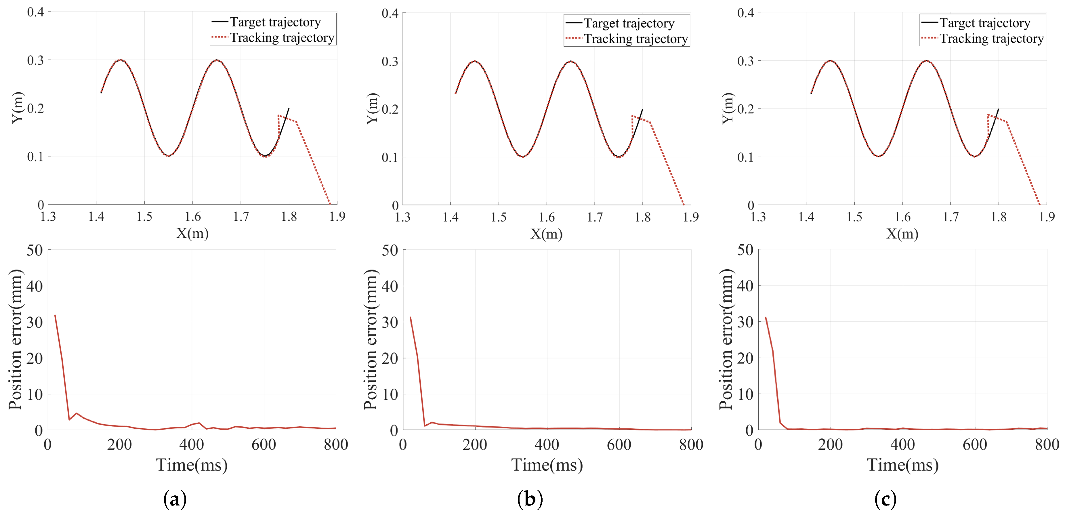
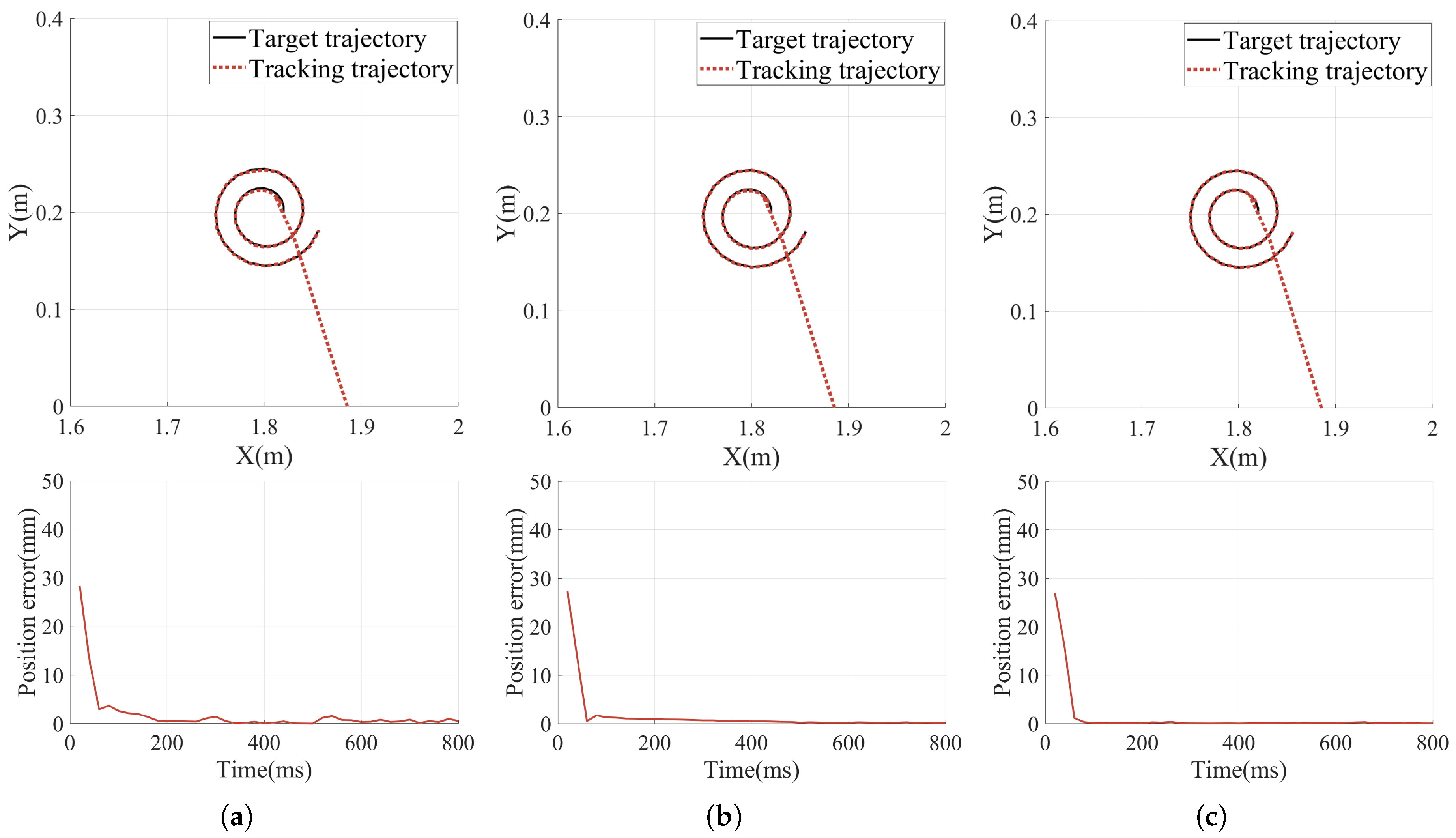
This simulation experiment is conducted based on two identical rotating prisms, with the setup illustrated in Figure 1. The apex angles are configured as ${\alpha }_1={\alpha }_2={10}^{\circ }$, and refractive indices are chosen as $n_1=n_2=1.5195$. Their initial angular positions are both set to ${\phi }_1\left(0\right)={\phi }_2\left(0\right)=0^{\circ }$, and the distance from the exit surface of prism 2 to the target plane is fixed at $D=10$ m. To validate the efficacy of TVMPDSC, its tracking performance is evaluated and compared against other methods for three distinct target trajectories: uniform linear, sinusoidal, and spiral, based on previously established prism and motor parameters. The uniform linear target maintains a constant linear velocity of 0.5 m/s. For the sinusoidal trajectory, target linear velocity varies periodically between 0.5 m/s and 1.6485 m/s. During spiral motion, target linear velocity increases monotonically from 0.315 m/s to 0.943 m/s. Moreover, the time step $T_d$ is set to 0.02 s. Comparative tracking results across all three control methods for these trajectories are presented in Figure 14, Figure 15 and Figure 16.

As observed in Figure 14, Figure 15 and Figure 16, in the presence of measurement noise and quantization errors, DVMPPC position error curves during linear, sinusoidal, and helical tracking exhibit the slowest convergence, accompanied by conspicuous continuous high-frequency position jitter during steady-state phases. Benefiting from three-vector optimization and seven-segment modulation strategies, TVMPPC achieves significantly improved error curve smoothness. However, owing to inherent integral lag effects within the outer-loop speed PI controller, TVMPPC lacks sufficient dynamic adaptability to guarantee high-performance tracking across wide speed ranges. Consequently, its actual trajectories consistently fail to perfectly match target profiles, resulting in persistent microscopic position deviations. In stark contrast, TVMPDSC not only demonstrates rapid position error convergence but also maintains exceptionally smooth error curves tightly adhering to the zero axes upon reaching steady states.

For a more comprehensive assessment of tracking performance across the three control methods, this study employs two key metrics: the integral of time-weighted absolute error (ITAE) and the integral of time-weighted squared error (ITSE), which can be defined as

$$\left\{\begin{array}{cc}\hfill \mathrm{ITAE}& =\sum _{i=1}^N{t}_i\left|e_i\right|\hfill \\ \hfill \mathrm{ITSE}& =\sum _{i=1}^N{t}_i{e}_i^2\hfill \end{array}\right.$$

(43)

where $t_i$ and $e_i$ denote the time instant and positional error at the i-th moment, respectively. The resultant values are listed in

Table 4. Tracking performance of different control methods.

Tracking Trajectory	Method	ITAE (mm·s)	ITSE (mm2$·$s)
Straight line	DVMPPC	10.54	42.03
	TVMPPC	7.12	36.01
	TVMPDSC	3.25	34.60
Sine line	DVMPPC	13.12	48.79
	TVMPPC	7.50	40.48
	TVMPDSC	5.22	39.87
Helical line	DVMPPC	11.01	33.35
	TVMPPC	7.53	26.10
	TVMPDSC	3.52	24.77

.

It can be observed that three tracking trajectories of TVMPDSC almost completely overlap with corresponding target trajectories. Compared to TVMPPC, TVMPDSC achieves a significant average reduction of 45.87% in ITAE and a slight decrease of 3.27% in ITSE across three trajectories. Compared to DVMPPC, TVMPDSC achieves average reductions of 65.42% and 20.08% in ITAE and ITSE across three trajectories, respectively. As a result, the proposed TVMPDSC method significantly enhances target tracking accuracy compared to DVMPPC while maintaining almost the same level of high target tracking stability as carefully tuned TVMPPC.

Although TVMPDSC exhibits exceptional target tracking performance and robustness under simulated hardware constraints, several practical limitations inherent in its physical implementation require acknowledgment. Primarily, because this control strategy derives reference active power directly from dynamic equations, the resulting control commands are directly coupled to the instantaneous quality of velocity feedback. Therefore, achieving absolute pointing stability during physical implementation strictly depends upon the position encoder’s physical resolution and signal integrity. Furthermore, inverter switching restrictions present another challenge. The employed three-vector seven-segment modulation strategy dictates precise execution of synthesized voltage vectors. However, within physical inverters, dead-time constraints and minimum on/off limitations of power semiconductor devices (e.g., MOSFETs) establish severe lower thresholds for synthesizable pulse widths. Such hardware boundaries may impede the exact execution of ultra-short active or zero vectors during rapid dynamic state transitions. Additionally, hardware deployment of this intricate predictive optimization algorithm requires executing massive floating-point matrix calculations and cost function assessments within a highly constrained control cycle (e.g., 50 $\mathsf{\mu }$s). This fundamental requirement exclusively limits the system to high-performance 32-bit floating-point DSPs, eliminating standard low-cost microcontrollers as viable alternatives. Finally, overall system tracking accuracy remains susceptible to unmodeled macroscopic mechanical nonlinearities within the Risley prism pair, such as temperature-dependent viscous friction and transmission backlash.

7. Conclusions

A three-vector-based model predictive direct speed control method for active power is introduced, aimed at achieving direct and precise speed regulation for BLDC motors within Risley prism systems. Based on the deadbeat power control principle, this approach directly generates reference active power through the system’s dynamic equations, establishing a direct control path from speed to torque. It achieves high-precision speed control across a wide speed range without requiring constant flux linkage approximation or parameter tuning. Meanwhile, it incorporates three-vector optimization and seven-segment PWM strategies, synthesizing a voltage vector closer to the ideal one within a single control cycle and enabling symmetrical output of inverter switching signals, thereby reducing motor losses without compromising speed stability. Through comparative simulation experiments on speed control of prism motor and dynamic target tracking under real-world hardware measurement constraints, the proposed control method is proven effective, with main conclusions summarized as follows:

(1)

The proposed control method achieves a dynamic balance between high-frequency and instantaneous fine-tuning of electromagnetic power and inherent mechanical inertia of the rotor. Relying on natural physical inertial damping, it ensures excellent speed stability.

(2)

The proposed control method demonstrates excellent robustness. Subjected to 30% stator inductance mismatches, 30% rotational inertia variations, or sudden 30% rated load impacts, it consistently maintains robust speed stability alongside high tracking precision.

(3)

During abrupt speed transitions, the proposed control method successfully avoids issues of PI parameter mismatch and integral windup that cause severe overshoots and lag in traditional cascaded structures. It achieves near-zero average speed deviations and zero-overshoot convergence within physical bandwidth, realizing wide-speed tracking adaptability that conventional methods cannot attain.

(4)

For three target trajectories, including uniform linear motion, sinusoidal motion, and helical motion, the proposed method achieves a high degree of overlap between the system’s actual tracking trajectory and the target trajectory. Specifically, it attains average reductions in ITAE and ITSE of 45.87% and 3.27% compared to TVMPPC, alongside 65.42% and 20.08% compared to DVMPPC. These results demonstrate the proposed control method significantly enhances target tracking accuracy compared to DVMPPC while maintaining almost the same level of high target tracking stability as carefully tuned TVMPPC.

References

1. Tan, C.; Kong, W.; Huang, G. Development of a near-infrared single-photon 3D imaging LiDAR based on 64 × 64 InGaAs/InP array detector and Risley-prism scanner. Opt. Express 2024, 32, 7426–7447. [Google Scholar] [CrossRef] [Scilit] [PubMed]
2. Li, A.; Ma, J.; Zhao, X. Advances in rotating Risley prisms for space-optics applications. Opt. Eng. 2025, 64, 080901. [Google Scholar] [CrossRef] [Scilit]
3. Mu, S.; Tan, S.; Qi, H. Optical System Design Method Based on Rotating Risley Prism. IEEE Photonics J. 2025, 17, 8600213. [Google Scholar] [CrossRef] [Scilit]
4. Peng, T.; Tao, M.; Ding, C. Multi-target free-space laser communication system based on a rotating double prism with an RF signal beacon. Opt. Express 2022, 30, 22221–22232. [Google Scholar] [CrossRef] [Scilit] [PubMed]
5. Chen, W.; Zhang, L.; Meng, L. Design and achromatic analysis of Risley-prism-based beam steering system for space laser communication. In Proceedings of the Third International Conference on Mechanical, Electronics, and Electrical and Automation Control (METMS 2023), Hangzhou, China, 18 July 2023; SPIE: Bellingham, WA, USA, 2023; Volume 12722, pp. 867–872. [Google Scholar] [CrossRef] [Scilit]
6. Hu, X.; Han, S.; Liu, Y. Two-Axis Optoelectronic Stabilized Platform Based on Active Disturbance Rejection Controller with LuGre Friction Model. Electronics 2023, 12, 1261. [Google Scholar] [CrossRef] [Scilit]
7. Wang, L.; Zhang, F.; Sun, H. High-dynamic tracking control technology for the fast-steering mirror in a laser communication system. Appl. Opt. 2025, 64, 8240–8247. [Google Scholar] [CrossRef] [Scilit]
8. Wu, Z.; Chen, Z.; Xue, L. Single detector compound axis system employs a two-axis mirror to achieve target acquisition. Opt. Express 2024, 32, 30500–30517. [Google Scholar] [CrossRef] [Scilit]
9. Xia, H.; Li, J.; Xia, Y. Multivariable decoupling and nonlinear correction method for image-based closed-loop tracking of the Risley prisms system. Micromachines 2022, 13, 2096. [Google Scholar] [CrossRef] [Scilit]
10. Xia, H.; Xia, H.; Li, J. Line-of-Sight Stabilization and High-Precision Target Tracking Technology of the Risley Prism System on Motion Platforms. Actuators 2025, 14, 240. [Google Scholar] [CrossRef] [Scilit]
11. Song, Y.; Gao, S.; Wu, J. Inverse Solution Error Analysis and Correction of Beam Steering System Based on Risley Prisms. Appl. Sci. 2022, 12, 1972. [Google Scholar] [CrossRef] [Scilit]
12. Zhou, Y.; Chen, Y.; Jiang, G. Nonlinearity Problem Analysis of Target Tracking Based on Rotational Double Prisms. Acta Opt. Sin. 2021, 41, 1823002–1823014. [Google Scholar] [CrossRef] [Scilit]
13. Yuan, L.; Huang, Y.; Fan, Y. Rotational Risley prisms: Fast and high-accuracy inverse solution and application based on back propagation neural networks. Measurement 2025, 242, 116007. [Google Scholar] [CrossRef] [Scilit]
14. Ma, R.; Wang, Q.; Xia, Y. Disturbance compensation of a multiaperture imaging system based on a coupling rotating prism using an improved model compensation control. Appl. Opt. 2021, 60, 4798–4806. [Google Scholar] [CrossRef] [Scilit] [PubMed]
15. Ma, R.; Wang, Q.; Li, J. Robust Risley prism control based on disturbance observer for system line-of-sight stabilization. Appl. Opt. 2022, 61, 3463–3472. [Google Scholar] [CrossRef] [Scilit] [PubMed]
16. Xing, R.; Xie, M.; Xue, H. Reinforcement Learning Compensatory-Based Fully Actuated Control Method for Risley Prisms. Photonics 2025, 12, 885. [Google Scholar] [CrossRef] [Scilit]
17. Masoudi, H.; Kiyoumarsi, A.; Madani, S.M. Torque ripple reduction of nonsinusoidal brushless dc motor based on super-twisting sliding mode direct power control. IEEE Trans. Transp. Electrif. 2023, 9, 3769–3779. [Google Scholar] [CrossRef] [Scilit]
18. Masoudi, H.; Kiyoumarsi, A.; Madani, S.M. Closed-loop direct power control of brushless dc motor in field weakening region. IEEE Trans. Transp. Electrif. 2023, 10, 3482–3491. [Google Scholar] [CrossRef] [Scilit]
19. Lee, S.K.; Kang, G.H.; Hur, J. Stator and rotor shape designs of interior permanent magnet type brushless DC motor for reducing torque fluctuation. IEEE Trans. Magn. 2012, 48, 4662–4665. [Google Scholar] [CrossRef] [Scilit]
20. Azarudeen, A.; Mary, D. Performance analysis of conventional and digital PWM control scheme for speed control of BLDC motor drives. In Proceedings of the 2017 International Conference on Advances in Electrical Technology for Green Energy (ICAETGT), Coimbatore, India, 23 September 2017; IEEE: Piscataway, NJ, USA, 2017; pp. 69–75. [Google Scholar] [CrossRef] [Scilit]
21. Lee, Y.; Kim, J. A novel enhanced inverted PWM driving scheme for three-phase BLDC motor drive. In Proceedings of the 2018 IEEE International Conference on Consumer Electronics-Asia (ICCE-Asia), JeJu, Republic of Korea, 24–26 June 2018; IEEE: Piscataway, NJ, USA, 2018; pp. 206–212. [Google Scholar] [CrossRef] [Scilit]
22. Chen, W.; Liu, Y.; Li, X. A novel method of reducing commutation torque ripple for brushless DC motor based on Cuk converter. IEEE Trans. Power Electron. 2016, 32, 5497–5508. [Google Scholar] [CrossRef] [Scilit]
23. Çorapsız, M.R.; Kahveci, H. Performance Analysis of Buck-Boost and SEPIC Converter for Commutation Torque Ripple Minimization in BLDC Motors. Electr. Power Compon. Syst. 2022, 49, 1052–1067. [Google Scholar] [CrossRef] [Scilit]
24. Shirvani Boroujeni, M.; Arab Markadeh, G.; Soltani, J. Torque ripple reduction of brushless DC motor with harmonic current injection based on integral terminal sliding mode control. IET Electr. Power Appl. 2018, 12, 25–36. [Google Scholar] [CrossRef] [Scilit]
25. He, J.; Yan, C.; Wang, X. Torque ripple suppression of brushless DC motor drive system based on improved harmonic injection active disturbance rejection control. Sensors 2022, 22, 1069. [Google Scholar] [CrossRef] [Scilit]
26. Ozturk, S.B.; Toliyat, H.A. Direct torque and indirect flux control of brushless DC motor. IEEE/ASME Trans. Mechatron. 2010, 16, 351–360. [Google Scholar] [CrossRef] [Scilit]
27. Heidari, R.; Markadeh, G.A.; Abazari, S. Direct torque and indirect flux control of brushless DC motor with non-sinusoidal back-EMF without position sensor. In Proceedings of the 2011 19th Iranian Conference on Electrical Engineering, Tehran, Iran, 17–19 May 2011; IEEE: Piscataway, NJ, USA, 2011; pp. 1–5. Available online: https://ieeexplore.ieee.org/abstract/document/5955539 (accessed on 15 January 2026).
28. Li, Z.; Zhang, S.; Zhou, S. Torque ripple minimization in direct torque control of brushless DC motor. J. Electr. Eng. Technol. 2014, 9, 1569–1576. [Google Scholar] [CrossRef] [Scilit]
29. Kumar, M.S.; Satheesh, G.; Peddakotla, S. Design of optimal PI controller for torque ripple minimization of SVPWM-DTC of BLDC motor. Int. J. Power Electron. Drive Syst. 2023, 14, 283–293. [Google Scholar] [CrossRef] [Scilit]
30. Kumar, P.; Bhaskar, D.V.; Behera, R.K. A modified torque ripple minimization technique for bldc motor drive using synthesized current phase compensation. In Proceedings of the 2020 IEEE International Conference on Industrial Technology (ICIT), Buenos Aires, Argentina, 26–28 February 2020; IEEE: Piscataway, NJ, USA, 2020; pp. 127–132. [Google Scholar] [CrossRef] [Scilit]
31. Xia, C.; Wang, Y.; Shi, T. Implementation of finite-state model predictive control for commutation torque ripple minimization of permanent-magnet brushless DC motor. IEEE Trans. Ind. Electron. 2012, 60, 896–905. [Google Scholar] [CrossRef] [Scilit]
32. Darba, A.; De Belie, F.; D’haese, P. Improved Dynamic Behavior in BLDC Drives Using Model Predictive Speed and Current Control. IEEE Trans. Ind. Electron. 2016, 63, 728–740. [Google Scholar] [CrossRef] [Scilit]
33. Li, Z.; Fan, X.; Kong, Q. Torque Ripple Suppression of BLDCM With Optimal Duty Cycle and Switch State by FCS-MPC. IEEE Open J. Power Electron. 2024, 5, 381–391. [Google Scholar] [CrossRef] [Scilit]
34. Emami, Z.; Niasar, A.H. Torque Ripple reduction of BLDC Motor Drive using Finite-Control-Set Model Predictive Control Strategy. In Proceedings of the 2023 3rd International Conference on Electrical Machines and Drives (ICEMD), Tehran, Iran, 20–21 December 2023; IEEE: Piscataway, NJ, USA, 2023; pp. 1–7. [Google Scholar] [CrossRef] [Scilit]
35. Buja, G.; Bertoluzzo, M.; Keshri, R.K. Torque ripple-free operation of PM BLDC drives with petal-wave current supply. IEEE Trans. Ind. Electron. 2014, 62, 4034–4043. [Google Scholar] [CrossRef] [Scilit]
36. Zhang, Y.; Xie, W.; Li, Z. Model Predictive Direct Power Control of a PWM Rectifier With Duty Cycle Optimization. IEEE Trans. Power Electron. 2013, 28, 5343–5351. [Google Scholar] [CrossRef] [Scilit]
37. de Castro, A.G.; Pereira, W.C.A.; Almeida, T.E.P. Improved finite control-set model-based direct power control of BLDC motor with reduced torque ripple. In Proceedings of the 2016 12th IEEE International Conference on Industry Applications (INDUSCON), Curitiba, PR, Brazil, 20–23 November 2016; IEEE: Piscataway, NJ, USA, 2016; pp. 1–6. [Google Scholar] [CrossRef] [Scilit]
38. de Castro, A.G.; Pereira, W.C.A.; de Almeida, T.E.P. Improved finite control-set model-based direct power control of BLDC motor with reduced torque ripple. IEEE Trans. Ind. Appl. 2018, 54, 4476–4484. [Google Scholar] [CrossRef] [Scilit]
39. Azab, M. Comparative Study of BLDC Motor Drives with Different Approaches: FCS-Model Predictive Control and Hysteresis Current Control. World Electr. Veh. J. 2022, 13, 112. [Google Scholar] [CrossRef] [Scilit]
40. Entezari, A.; Kolagar, A.D.; Alizadeh, M.R. Direct Power Control in BLDC Motor Drives Using Finite Control Set Model Predictive Control to Reduce Torque Ripple and Speed Fluctuation and Improve Harmonic Distortions. J. Control 2024, 17, 1–19. [Google Scholar]
41. Xu, Y.; Li, S.; Zhang, W. Long-Horizon Constrained Model Predictive Direct Speed Control for PMSM Drives Based on Laguerre Functions. IEEE Trans. Control Syst. Technol. 2024, 32, 1002–1014. [Google Scholar] [CrossRef] [Scilit]
42. Zhao, M.; Cao, Y.; Li, C. Expanded Limit Boundary Explicit Model Predictive Direct Speed Control for PMSMs. IEEE Trans. Power Electron. 2024, 39, 6089–6101. [Google Scholar] [CrossRef] [Scilit]
43. Zerdali, E.; Rivera, M.; Riccio, J. Direct Speed Predictive Control of an Induction Motor. In Proceedings of the IECON 2024-50th Annual Conference of the IEEE Industrial Electronics Society, Chicago, IL, USA, 3–6 November 2024; IEEE: Piscataway, NJ, USA, 2024; pp. 1–5. [Google Scholar] [CrossRef] [Scilit]
44. Zerdali, E.; Riccio, J.; Rivera, M. Sensorless model predictive direct speed control of an induction motor. In Proceedings of the 13th International Conference on Power Electronics, Machines and Drives (PEMD 2024), Nottingham, UK, 10–13 June 2024; IET: London, UK, 2024; pp. 398–403. [Google Scholar] [CrossRef] [Scilit]
45. Li, Y. Closed form analytical inverse solutions for Risley-prism-based beam steering systems in different configurations. Appl. Opt. 2011, 50, 4302–4309. [Google Scholar] [CrossRef] [Scilit]
46. Zhou, Y.; Chen, Y.; Sun, L. Singularity Problem Analysis of Target Tracking Based on Risley Prisms. Acta Opt. Sin. 2025, 45, 0312001–0312011. [Google Scholar] [CrossRef] [Scilit]
Figure 1. Schematic diagram of beam deflection by the Risley prism pair. (a) Three-dimensional beam deflection diagram. (b) One possible configuration of prism pair.
Actuators 15 00213 g001
Figure 2. Schematic diagram of target tracking.
Actuators 15 00213 g002
Figure 3. Equivalent circuit of BLDC motor.
Actuators 15 00213 g003
Figure 4. The control structure of the proposed method.
Actuators 15 00213 g004
Figure 5. Voltage vectors and sectors of two-level VSI.
Actuators 15 00213 g005
Figure 6. The results of A-phase current waveform and total harmonic distortion. (a) DVMPPC. (b) TVMPPC. (c) TVMPDSC.
Actuators 15 00213 g006
Figure 7. The results of active power, reactive power, and torque. (a) DVMPPC. (b) TVMPPC. (c) TVMPDSC.
Actuators 15 00213 g007
Figure 8. The results of output speed. (a) DVMPPC. (b) TVMPPC. (c) TVMPDSC.
Actuators 15 00213 g008
Figure 9. Torque and speed responses under 30% L s increase. (a) DVMPPC. (b) TVMPPC. (c) TVMPDSC.
Actuators 15 00213 g009
Figure 10. Torque and speed responses under 30% load increase. (a) DVMPPC. (b) TVMPPC. (c) TVMPDSC.
Actuators 15 00213 g010
Figure 11. Torque and speed responses under 30% J increase. (a) DVMPPC. (b) TVMPPC. (c) TVMPDSC.
Actuators 15 00213 g011
Figure 12. Tracking results of different control methods at different reference speeds.
Actuators 15 00213 g012
Figure 13. Architecture of the control system.
Actuators 15 00213 g013
Figure 14. Tracking trajectories and position errors for the uniform linear motion target. (a) DVMPPC. (b) TVMPPC. (c) TVMPDSC.
Actuators 15 00213 g014
Figure 15. Tracking trajectories and position errors for the sinusoidal motion target. (a) DVMPPC. (b) TVMPPC. (c) TVMPDSC.
Actuators 15 00213 g015
Figure 16. Tracking trajectories and position errors for the helical motion target. (a) DVMPPC. (b) TVMPPC. (c) TVMPDSC.
Actuators 15 00213 g016