1. Introduction
Proportional–integral–derivative (PID) controllers continue to serve as a benchmark feedback control strategy in industrial and engineering practice because of their structural simplicity, ease of implementation, and reliable closed-loop behavior across a broad class of systems. Despite the availability of advanced control methodologies, PID controllers dominate practical applications in process control, power systems, robotics, and biomedical engineering [
1,
2,
3]. Their ongoing relevance stems from the fact that they offer a satisfactory control performance, computational simplicity, and interpretability [
4].
The PID control is successful if its gains are properly selected. Poorly tuned gains may lead to slow responses, excessive overshoot, oscillatory behavior, large control effort, or even instability. For this reason, PID tuning has remained a central topic in control engineering for decades. Classical tuning rules, such as the Ziegler–Nichols, Cohen–Coon and SIMC [
5] methods, provide simple heuristic procedures for obtaining gain. Although these methods are attractive for their simplicity, they are primarily intended for relatively simple linear plants and often fail in the presence of actuator limitations, nonlinear dynamics, or application-specific performance requirements. Their effectiveness therefore decreases when the control problem involves nonconvex performance landscapes, strict safety constraints, or substantial model nonlinearities [
6,
7,
8].
To overcome these limitations,
optimization-based PID tuning methods have come forward [
9]. In such approaches, the controller gains are selected by minimizing an objective function defined in terms of the tracking error, control effort, settling behavior, overshoot, or other closed-loop performance measures. Gradient-based methods can be effective when the objective function is smooth and well-behaved, but they are often less suitable for simulation-based tuning problems involving saturation, nonsmooth penalties, or nonlinear dynamics. Consequently, population-based metaheuristic algorithms [
10], such as genetic algorithms (GA), particle swarm optimization (PSO), differential evolution [
11], and related evolutionary strategies have become popular alternatives for PID tuning. More recently, nature-inspired algorithms such as the grey wolf optimizer [
12] and whale optimization algorithm [
13] have also been applied to PID tuning. Because of their derivative-free nature, these methods are attractive and can explore broad search spaces. However, their performance depends strongly on the evaluation budget and algorithmic parameter selection, and they may require a large number of expensive objective evaluations before converging to a satisfactory solution [
10,
14].
In parallel with metaheuristic approaches, model-free optimal tuning methods have been developed that do not require an explicit plant model. Iterative feedback tuning [
15] directly minimizes a performance criterion using closed-loop gradient estimates obtained from special experiments. Extremum seeking [
16] treats the performance metric as a cost surface and uses sinusoidal perturbations to estimate its gradient in real time. Virtual reference feedback tuning [
17] computes controller parameters from a single batch of input–output data. More recently, Bayesian optimization has been applied to PID tuning [
18], using Gaussian process surrogates with expected improvement acquisition functions. These methods are particularly effective for low-dimensional problems. However, they generally do not provide a reusable global model of the cost landscape, nor do they offer explicit exploration–exploitation separation across the parameter space.
These issues are especially relevant when each evaluation of the objective function requires the time-domain simulation of a nonlinear closed-loop system. In such settings, the computational burden of repeated direct evaluations becomes significant, particularly when actuator constraints, state penalties, or safety-oriented performance terms are included into the cost function. Surrogate-based optimization provides a different way to address this difficulty. Instead of relying exclusively on the direct sampling of the true objective function, surrogate-based methods [
19] construct an approximate model of the performance landscape from previously evaluated samples and use this approximation to guide the search toward promising regions of the parameter space. This strategy is particularly attractive for PID tuning because the dimension of the gain vector is low, while the underlying cost surface may still be highly nonlinear, multimodal, and expensive to evaluate.
Motivated by this observation, this paper investigates a surrogate-based optimization via clustering (SBOC) [
20] framework for systematic PID tuning. The central idea is to replace a purely blind search with a guided search process that combines objective evaluation, the clustering-based structural interpretation of the sampled gain space, and surrogate-assisted candidate refinement [
21]. In contrast to classical rule-based tuning, the proposed framework does not assume a specific analytical tuning formula. In contrast to purely population-based metaheuristics, it is designed to exploit the information contained in previously evaluated samples so that the search effort can be concentrated more effectively in promising regions. The framework is intended to remain general across different plant classes. At the same time, it preserves a uniform PID design structure throughout all case studies.
The prime objective of this work is not merely to tune PID controllers for a one class of control system problems, but to examine whether a unified SBOC-based tuning strategy can produce meaningful and interpretable controller structures across systems of increasing complexity. Therefore, the proposed methodology is validated on four representative problems: a first-order linear time-invariant (LTI) system, a second-order under-damped LTI system, a nonlinear pendulum with actuator saturation, and a blood glucose regulation problem based on the Bergman minimal model (BMM) [
22,
23] for type 1 diabetes. We thus verified the effectiveness of the framework on the systems with substantially different dynamic characteristics, ranging from simple monotonic dynamics to oscillatory, nonlinear, and safety-critical physiological behavior. This sequence of case studies enables a structured examination of how the tuned PID gains evolve as system complexity increases. It is notable that the proposed SBOC-based procedure aims to reveal not only the final controller performance but also the search process structure, the clustering patterns of candidate gains, and the way optimized PID gains reflect the underlying dynamics of each plant.
The main contributions of this paper are summarized as follows:
- (i)
A machine intelligence framework coupling SBOC with PID tuning is developed, in which the optimizer autonomously discovers the appropriate controller structure (PI, PID, or PD) for each plant without imposing any structural constraints a priori.
- (ii)
A safety-aware multi-objective cost function is formulated that integrates tracking quality, transient behavior, control effort, and asymmetric safety penalties into a single optimization objective, with demonstrated effectiveness in the safety-critical diabetes application.
- (iii)
The method is validated progressively on first-order, second-order, nonlinear pendulum, and physiological benchmarks (the blood glucose regulation problem), establishing practical guidelines for when to expect PI, PID, or PD structures based on the underlying plant physics.
- (iv)
A comparative analysis against widely used optimization-based tuning approaches is included to assess the competitiveness of the proposed method under a common evaluation budget setting.
The remainder of this paper is organized as follows.
Section 2 introduces the modeling framework for systems.
Section 3 presents the SBOC methodology and the optimization formulation used for PID tuning.
Section 4 reports and discusses the tuning results for the first-order, second-order, nonlinear pendulum, and physiological case studies in
Section 5. The comparative study with GA and PSO is conducted in
Section 6.
Section 7 concludes the paper and highlights the future scope of research.
3. Surrogate-Based Optimization via Clustering (SBOC)
The SBOC algorithm, originally developed for the global optimization of box-constrained systems [
20], is adapted here for PID parameter tuning. It constructs a single global surrogate model (a statistical model that approximates the output of the function accurately based on the specific set of inputs) at each iteration and uses
k-means clustering to distinguish well-sampled regions from under-explored areas. In this way, it balances the exploration and exploitation in the PID parameter space.
3.1. Notation and Overview
Let
N denote the number of decision variables (here,
corresponding to
,
, and
). The feasible domain
is normalized to the unit hypercube
. At iteration
i, let
denote the current dataset comprising
sample points and their objective values. Define the incumbent best solution and its objective value as
At each iteration, SBOC attempts to add up to three new sample points: one via surrogate minimization (exploitation), one via inter-cluster exploration, and one via local neighborhood refinement. The algorithm terminates when the total number of function evaluations reaches the budget .
3.2. Initial Sampling
SBOC generates
initial sample points in
using the Sobol quasi-random sequence [
27], which provides superior space-filling coverage compared to pseudo-random sampling or grid-based designs. Sobol sequences are deterministic low-discrepancy sequences that provide superior space-filling uniformity compared to both pseudo-random sampling and Latin hypercube designs [
27]. The deterministic nature eliminates initialization sensitivity: given the same dimension
N, every run begins with identical initial coverage of the domain. The objective function
is evaluated at each sample point via closed-loop simulation, yielding the initial dataset:
3.3. Surrogate Model Construction
At each iteration
i, a radial basis function (RBF) surrogate
is constructed from the current dataset
. This surrogate provides an inexpensive approximation of the true cost function. The RBF interpolant is defined as
where the multiquadric basis function is
and the linear polynomial tail is
Here,
is a shape hyperparameter,
(
) are the RBF coefficients, and
(
) are the polynomial coefficients.
The unknown parameters
and
are determined by solving the
symmetric block system:
where
has entries
, the polynomial matrix is
, and
. This formulation guarantees exact interpolation at all sample points.
The hyperparameter is selected via cross-validation from ten equi-spaced values in the interval . For each candidate value, a surrogate is trained on a randomly selected 80% of the data and its prediction accuracy is assessed on the remaining 20%. This procedure is repeated five times with different random splits, and the yielding the lowest mean squared prediction error is selected. The final surrogate is then trained on the full dataset using this optimal .
Note 4. The surrogate employed in this work is a deterministic RBF interpolant, which should be distinguished from Kriging (Gaussian process) surrogates. Unlike Kriging, the RBF interpolant does not provide a posterior variance estimate for uncertainty quantification. Instead, the exploration of uncertain (sparse data) regions is handled explicitly through the K-means clustering mechanism (Section 3.5), which identifies under-sampled inter-cluster gaps and places new evaluation points in these regions. This structural exploration mechanism serves an analogous role to the variance-based exploration in expected improvement criteria, without requiring the overhead of Gaussian process hyperparameter optimization. The only hyperparameter in the RBF surrogate is the shape parameter ψ, which is selected automatically via five-fold cross-validation at each iteration, requiring no manual tuning. 3.4. Surrogate Minimization
The surrogate model
is minimized over
using a multi-start strategy. A sequential quadratic programming solver is initialized from each of the existing sample points
,
:
The minimizer
is added to
only if it satisfies a minimum separation criterion from all the existing sample points:
If this condition is not met, the point is discarded to avoid the clustering of points and numerical ill conditioning of the RBF system. This step constitutes the primary exploitation mechanism of SBOC.
3.5. K-Means Clustering with Elbow Method
To identify the under-explored regions of the domain, the sample points in
are partitioned into
clusters using the
k-means algorithm [
28]. The optimal number of clusters is determined automatically at each iteration via the elbow method [
29]. Let
denote the total intra-cluster squared distance for
C clusters. The optimal cluster count is
This criterion identifies the cluster count beyond which marginal reductions in TICSD become insignificant. It thereby provides an automated and adaptive partitioning of the parameter space at each iteration.
3.6. Exploration of Vacant Sub-Spaces
The clustering step partitions the sample points into groups, but the objective is to identify large inter-cluster gaps devoid of sample points. For each cluster
, its nearest neighbor cluster
is identified based on the inter-cluster distance (ICD):
where
and
denote the sets of points in clusters
u and
v, respectively. Among all the nearest-neighbor cluster pairs, the pair
with the largest ICD is selected. The boundary points
and
defining this distance are identified, and the second new point is placed at their midpoint:
This heuristic efficiently identifies under-sampled regions without requiring expensive geometrical constructions such as Delaunay triangulations. The point is evaluated via closed-loop simulation and added to the dataset, constituting the exploration mechanism of SBOC.
3.7. Local Exploitation Around the Best Point
To refine the incumbent solution, a new point is generated in the local neighborhood of
. Define the local neighborhood
as the nearest
sample points based on Euclidean distance. Each neighbor
is assigned a Gaussian weight:
where
controls the sensitivity of the weights to variations in objective value. A smaller
concentrates the weight on points with objective values closest to
, while a larger
distributes weight more uniformly.
The third new point is computed as the weighted average:
Critically, is not fixed but cycles through the values across successive iterations. This periodic variation ensures that new points are not repeatedly placed at identical locations, particularly when does not improve over consecutive iterations.
3.8. Termination and Algorithm Summary
The iterative process of surrogate construction, clustering, exploration, and exploitation continues until the total number of function evaluations reaches
. The overall SBOC procedure is summarized in Algorithm 1.
| Algorithm 1 SBOC for PID tuning |
- Require:
Objective function , bounds , , budget - 1:
Generate initial points via Sobol sampling in - 2:
Evaluate for via closed-loop simulation - 3:
Initialize , identify and - 4:
Set iteration counter - 5:
while total evaluations do - 6:
Surrogate: Train RBF model on with cross-validated - 7:
Point 1 (Exploit): Minimize via multi-start SQP - 8:
Add to if separation - 9:
Cluster: Determine via elbow method; apply k-means to - 10:
Point 2 (Explore): Place midpoint in largest inter-cluster gap - 11:
Evaluate and add to - 12:
Point 3 (Refine): Compute weighted average in with cyclic - 13:
Evaluate and add to - 14:
Update , ; set - 15:
end while - 15:
return as the optimal PID gains
|
3.9. Key Algorithmic Features
Several features of SBOC which make it well-suited for PID tuning as follows:
- (i)
Model agnostic. While RBF surrogates are employed in this work, the framework is compatible with any surrogate modeling technique (e.g., Kriging [
30], polynomial regression [
31], and neural networks).
- (ii)
Single global surrogate. Unlike methods that construct multiple local surrogates for different subregions, SBOC works on a single surrogate over the entire domain. This reduces the complications related to domain partitioning, surrogate overlap, and boundary effects.
- (iii)
Explicit exploration–exploitation separation. Each iteration generates three points with distinct roles: (i) the surrogate minimizer for exploitation, (ii) the inter-cluster midpoint for exploration, and (iii) the weighted neighborhood average for local refinement. This is in contrast to methods based on expected improvement or weighted metrics that implicitly balance exploration and exploitation through a single criterion.
- (iv)
Computational efficiency. Clustering via k-means is computationally inexpensive compared to geometrical constructions such as Delaunay triangulations. This enables the deployability of SBOC framework to higher-dimensional parameter spaces.
- (v)
Physics through simulation. The SBOC surrogate is a black box approximation of the cost landscape and does not encode physical laws directly. However, physical constraints (for example, actuator saturation, non-negative control inputs, state bounds, and safety penalties) are enforced through the closed-loop simulation that evaluates each candidate. The surrogate approximates the resulting cost, which already reflects all the physical effects. This separation of concerns allows the framework to be applied to any system for which a simulation (or experimental evaluation) is available, without requiring an analytical plant model.
4. Validation on Benchmark Systems
We now apply the proposed SBOC-based PID tuning framework on different class of dynamical systems.
4.1. First-Order Linear System
Consider a first-order LTI plant described by the transfer function:
where
is the static gain and
s is the time constant. This system represents a broad class of industrial processes, including thermal systems, chemical reactors, and flow control loops, and serves as a baseline for validating the proposed framework.
The control objective is to regulate the system output
to a unit step reference (
) using a PID controller with a derivative filter (
). The PID gains are constrained to the following bounds:
The closed-loop transfer functions from the reference to the output and from the reference to the control input are, respectively, as follows:
where
denotes the PID controller transfer function.
The cost function for this system is defined as
where the simulation horizon is
s (=20
) and the settling penalty
is applied if
for any
. The specific values of the weighting coefficients and penalty parameters used for this system are
Note 5. This configuration indicates low overshoot and fast settling while lightly penalizing the control effort. The designer may adjust these weights according to the specific performance requirements of the application.
The SBOC algorithm is configured with
decision variables,
initial Sobol sample points, and a total evaluation budget of
. The RBF surrogate employs the multiquadric basis function (
18) with cross-validated
.
The SBOC algorithm was executed with the above configuration. The optimal PID gains obtained are
yielding a minimum cost of
after 120 function evaluations.
It is notable that the optimizer converged to , thereby yielding a proportional–integral (PI) controller. This result is physically consistent with the first-order plant dynamics: since the system has no oscillatory modes or second-order effects, derivative action provides no benefit for improving transient response. The optimizer autonomously identified this structural insight without any a priori constraint on the controller order, demonstrating the ability of the surrogate-based framework to discover the most appropriate controller structure from data.
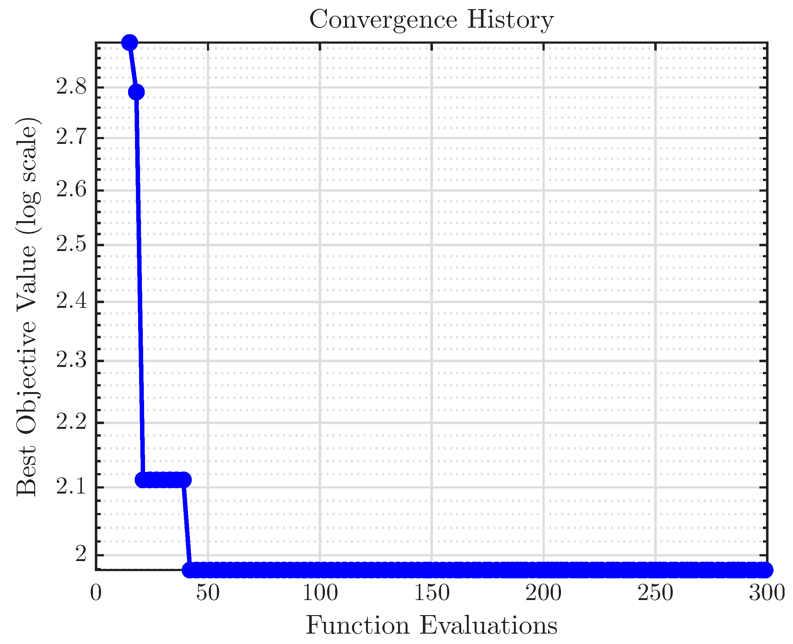
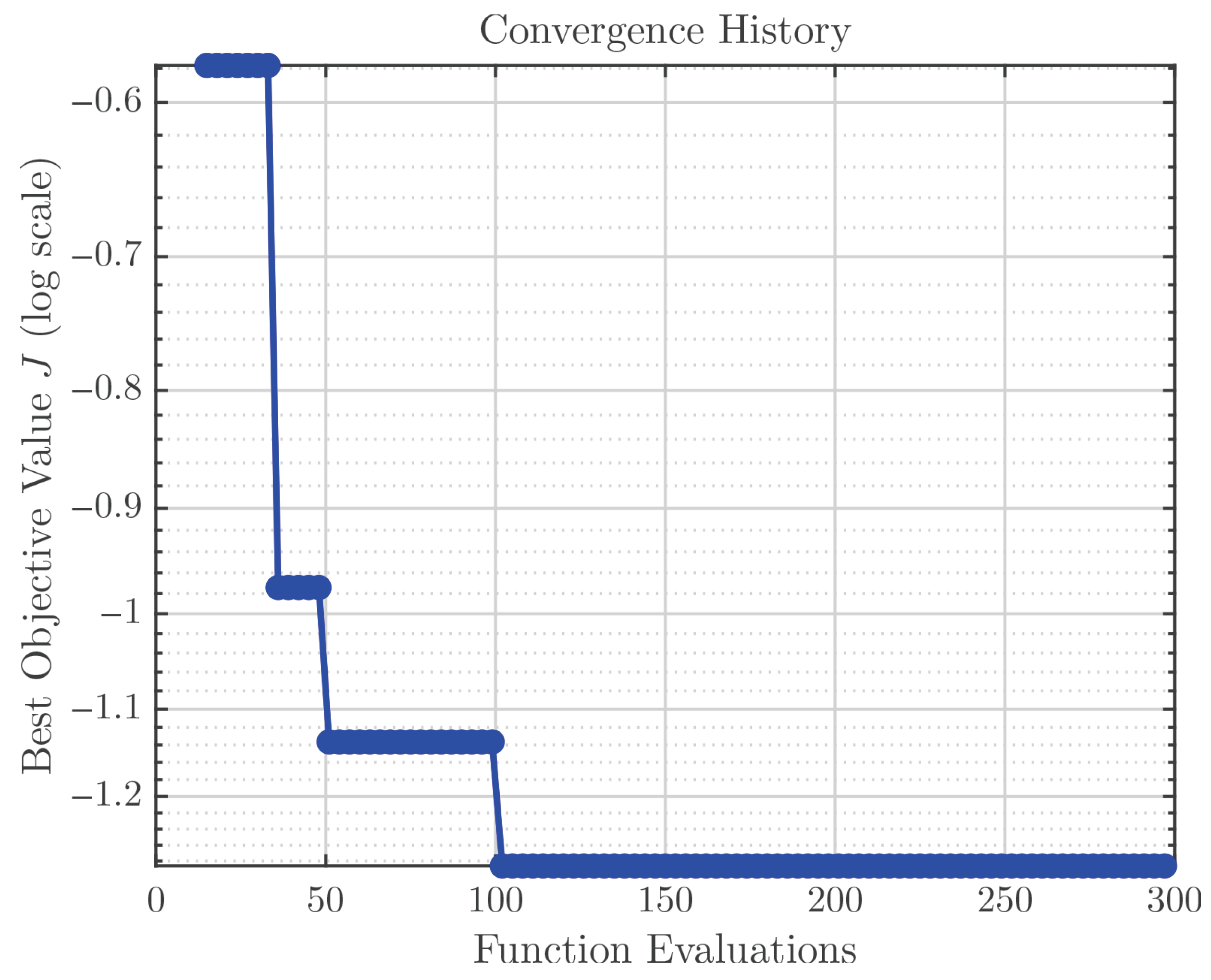
Figure 1 presents the convergence history of the SBOC algorithm. The best objective value decreases rapidly during the initial iterations, achieving near-optimal performance within approximately 20 evaluations. Subsequently, the algorithm continues refining the solution through its exploration and exploitation mechanisms. The rapid initial convergence can be attributed to the quality of the RBF surrogate, which provides an accurate approximation of the cost surface from the well-distributed Sobol initial samples.
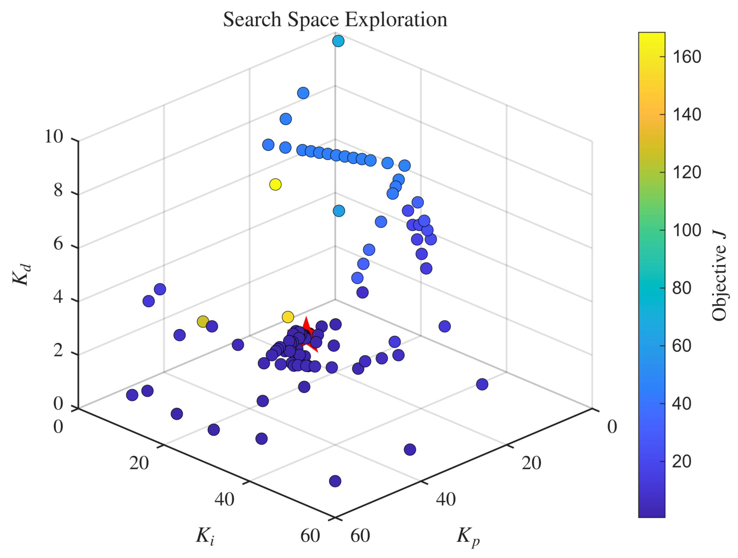
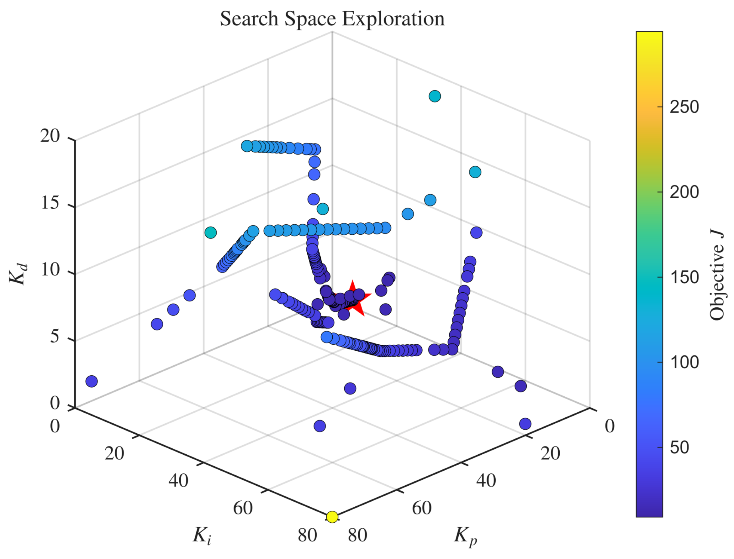
The 3D scatter plot of all the evaluated points in
Figure 2 illustrates the distribution of sample points across the PID gain space. The color intensity reflects the objective value at each point, showing that SBOC concentrated its evaluations in the low-
region where the optimum was located, while also exploring diverse regions of the parameter space to ensure global coverage.
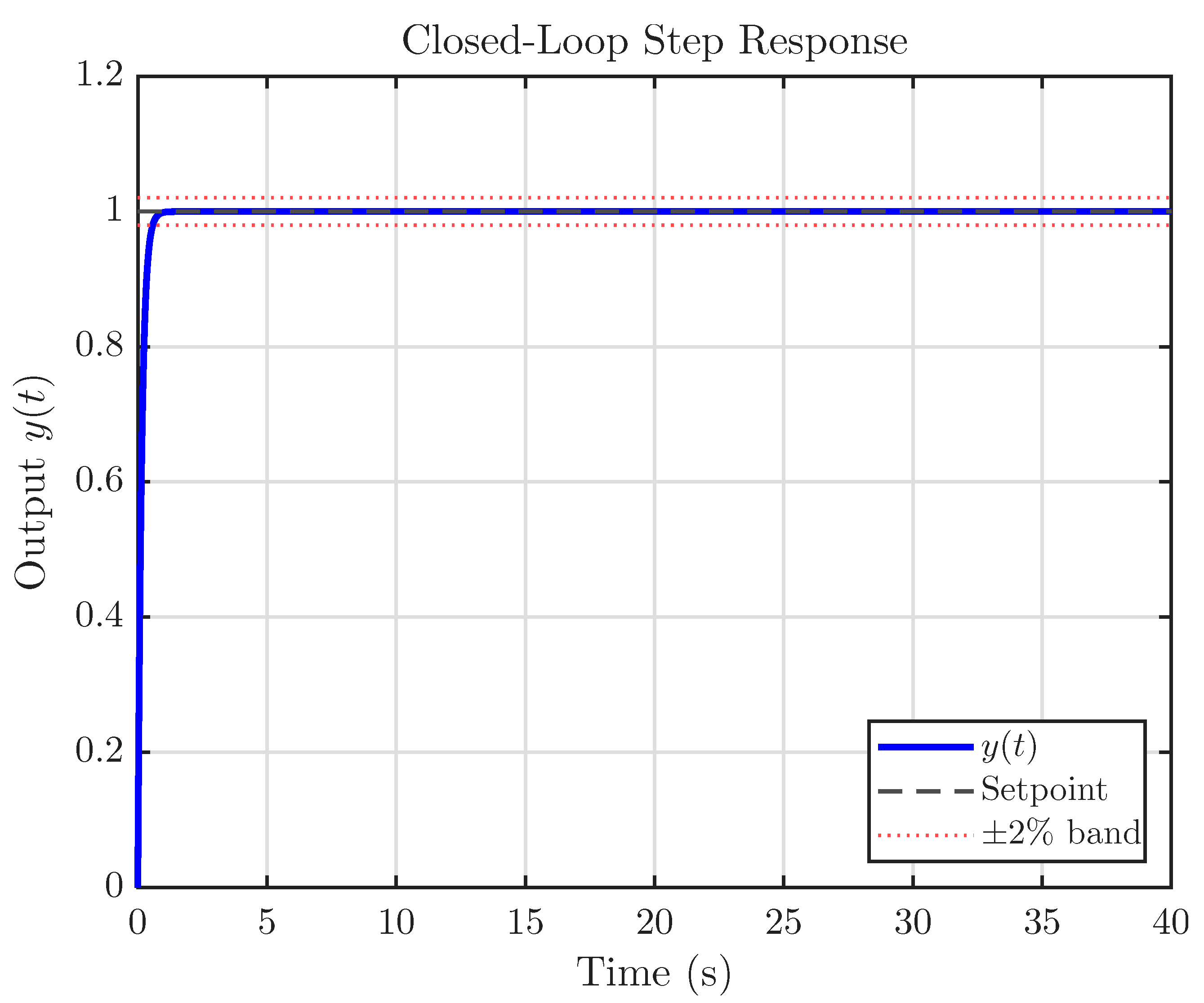
The step response of the closed-loop system under the SBOC-optimized PID controller is shown in
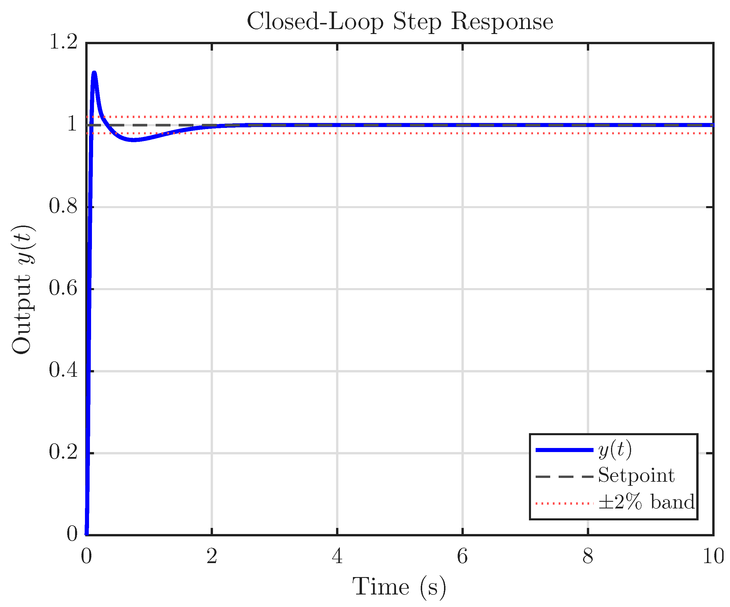
Figure 3. The response exhibits a fast rise time, negligible overshoot, and smooth convergence to the setpoint. The output enters and remains within the
settling band within approximately 5 s, corresponding to
, which represents good performance for a first-order plant.
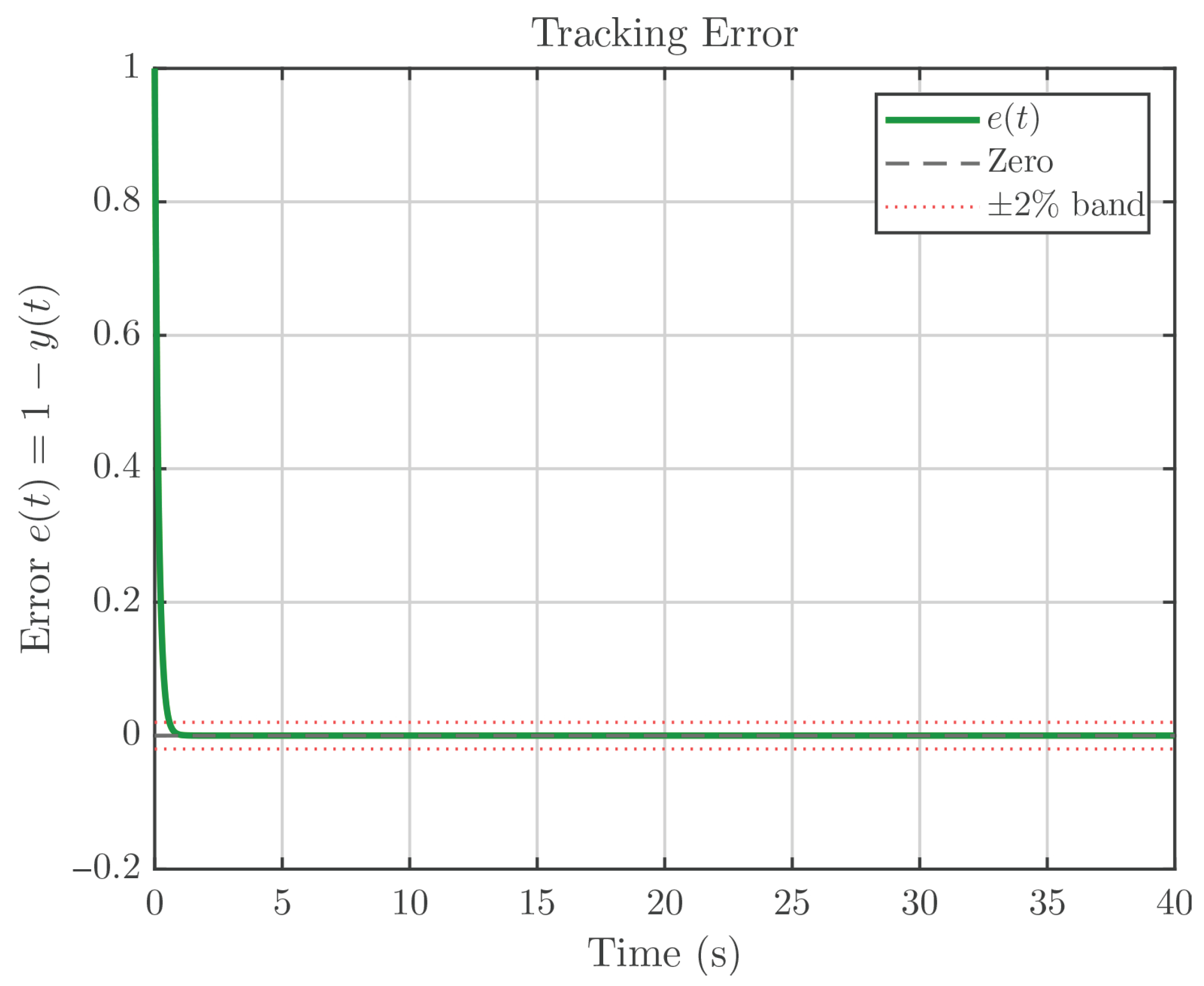
Figure 4 shows the tracking error
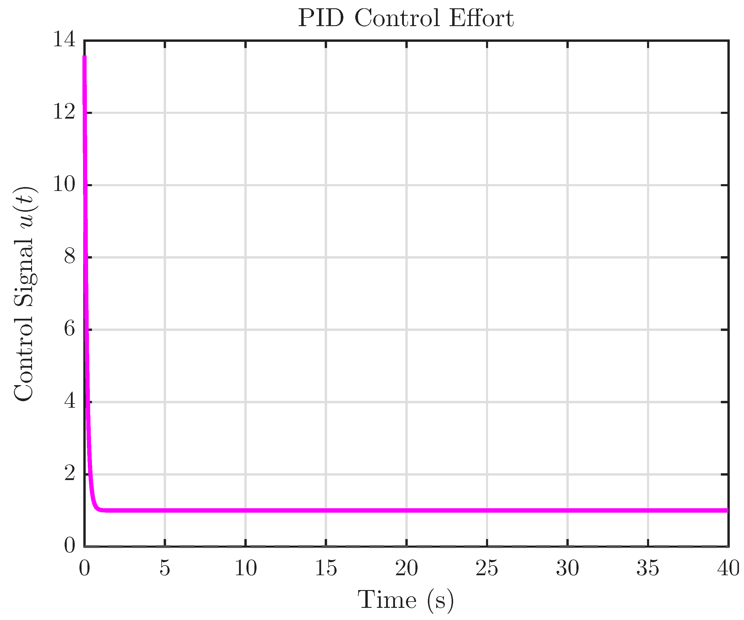
, which decays monotonically from unity to zero without any oscillatory behavior, confirming the effectiveness of the PI-type controller identified by SBOC. The control signal depicted in
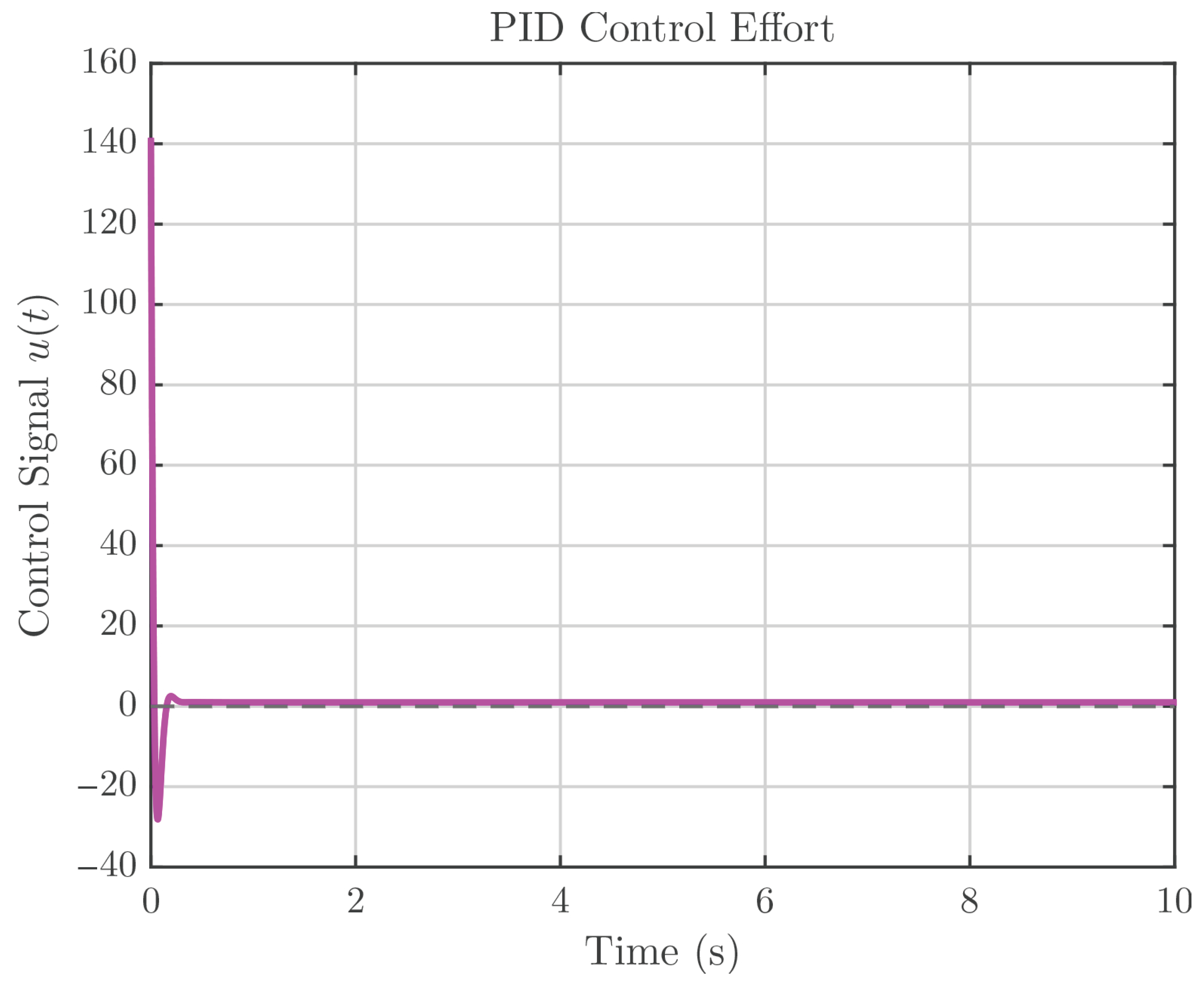
Figure 5 shows a moderate initial peak followed by smooth decay to the steady state, indicating well-behaved actuator usage without aggressive transients.
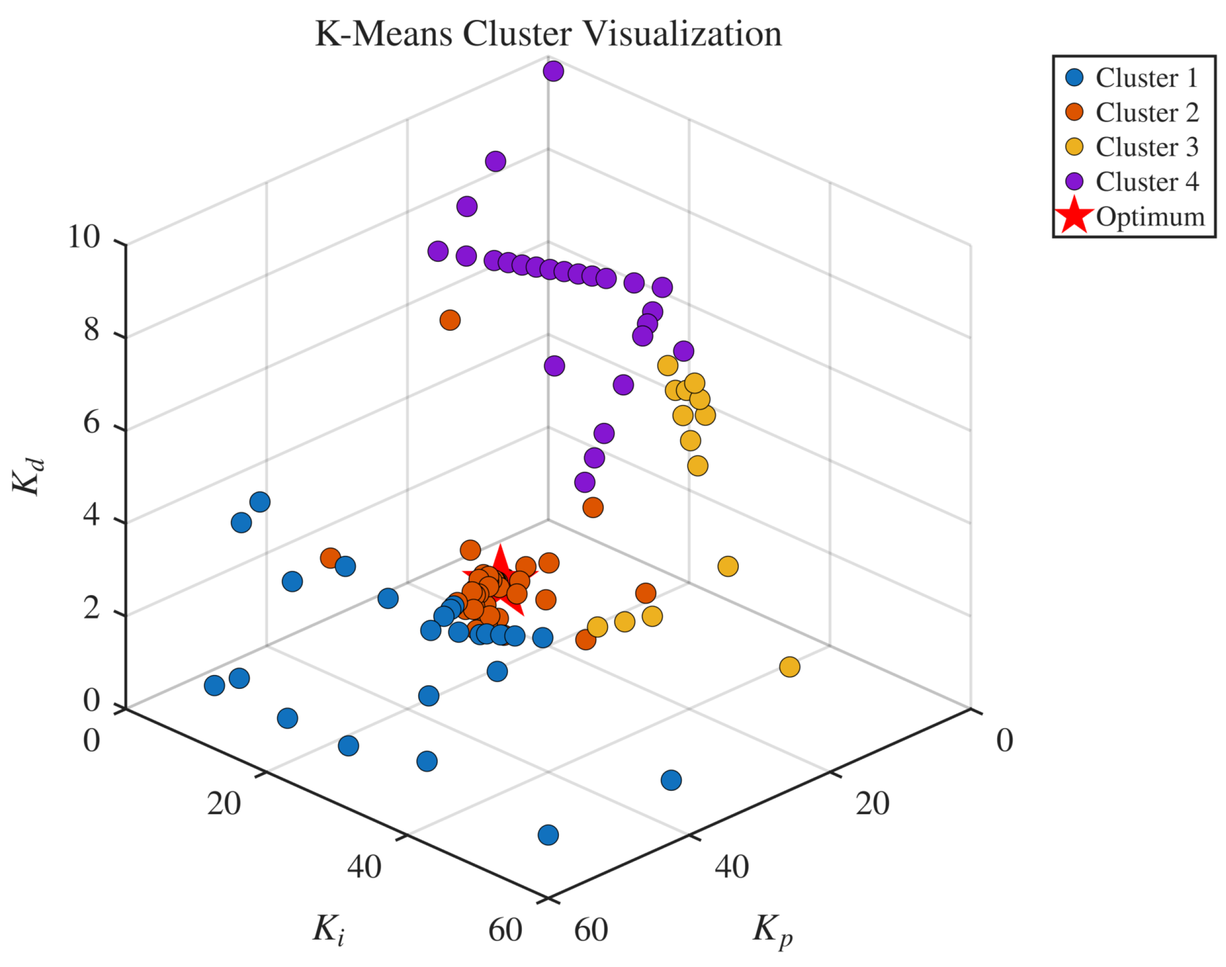
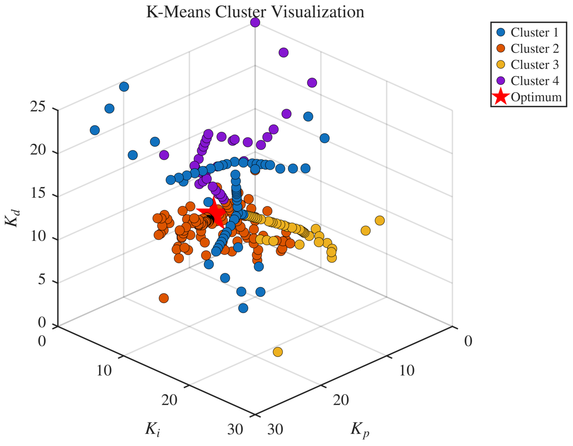
Figure 6 presents the
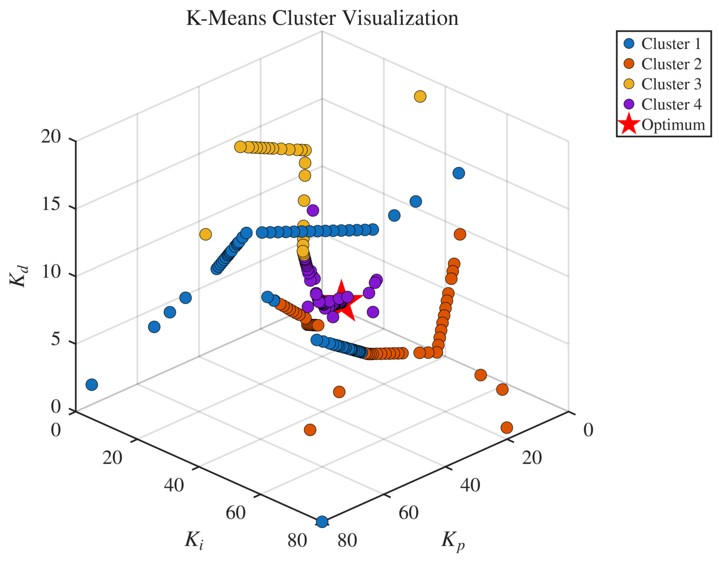
k-means cluster visualization of the final sample point distribution. Four distinct clusters are visible in the PID gain space, with the optimal solution (red star) located in the cluster corresponding to moderate
, low
, and near-zero
. The spatial separation between the clusters confirms that the exploration step effectively sampled diverse regions of the parameter space, while the exploitation step refined the search around the most promising area.
4.2. Second-Order Linear System
Let us consider a second-order LTI system described by the transfer function:
where
rad/s is the natural frequency and
is the damping ratio. This configuration corresponds to a lightly damped system exhibiting significant oscillatory behavior, with an open-loop overshoot of approximately 52.6% and a poorly damped transient response. Such dynamics are representative of flexible mechanical systems, lightly damped electrical circuits, and under-damped process control applications.
Similarly to the first-order case, the control objective is to regulate
to a unit step reference using a PID controller with derivative filter (
). The PID gains are bounded as
Here, we select the wider bounds in comparison to the first-order system to accommodate the larger gain values that may be required to adequately damp the oscillatory plant dynamics.
Similar to the first-order system, the cost function is framed as
with the simulation horizon set to
s and the same weighting coefficients as given in (
32).
The algorithm is configured with , initial Sobol points, and the evaluation budget . The larger budget relative to the first-order system reflects the increased complexity of the oscillatory cost landscape, which contains multiple local minima due to the interplay between proportional, integral, and derivative actions on a lightly damped plant.
The optimal PID gains obtained by SBOC are
yielding a minimum cost of
after 300 function evaluations.
Unlike the first-order system where , the optimizer here identified a non-zero derivative gain . This result is physically consistent because the lightly damped second-order plant requires derivative action to provide additional damping and suppress oscillatory transient behavior. The optimizer independently discovered this structural requirement without any a priori guidance regarding the necessity of derivative control.
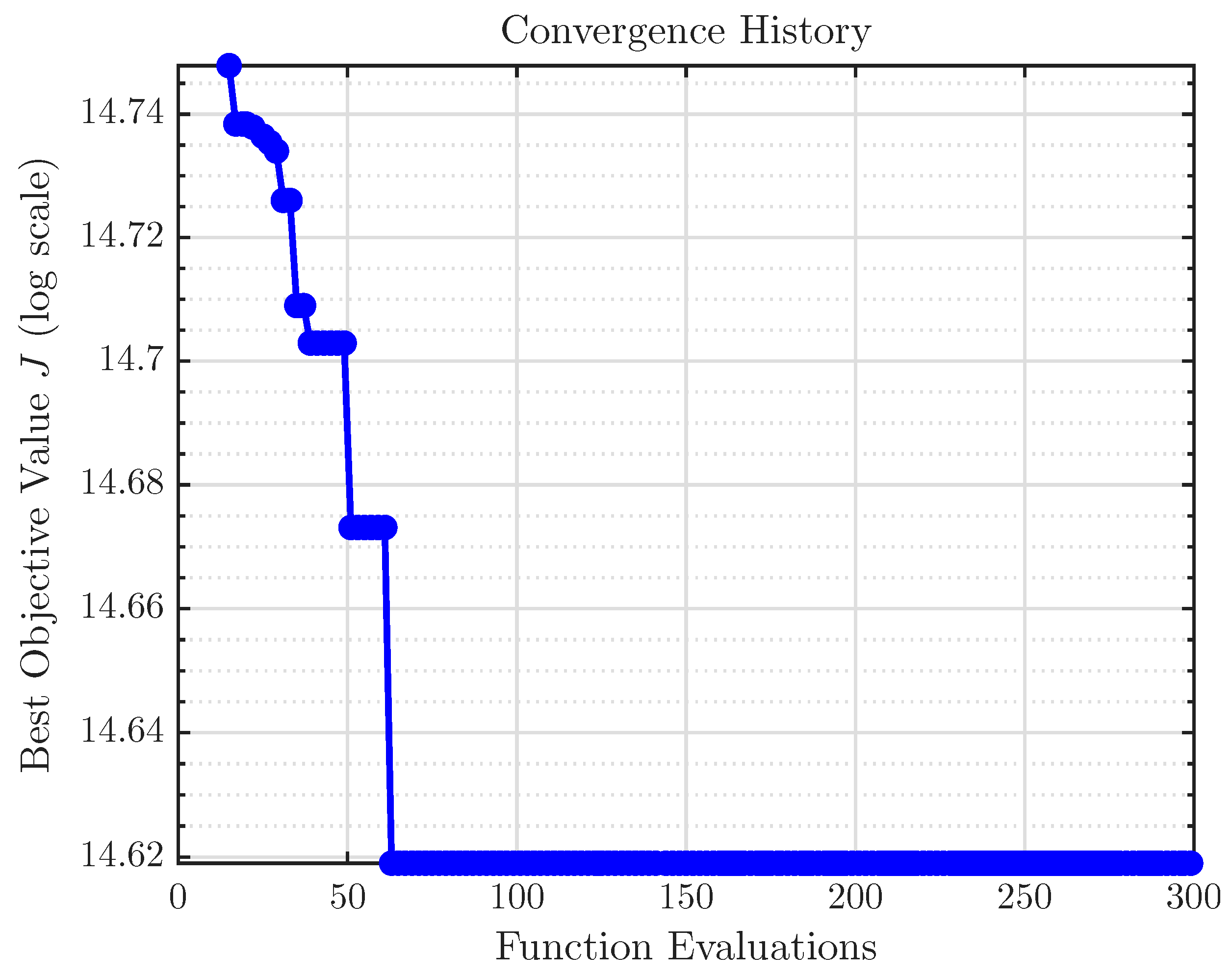
Figure 7 presents the convergence history for the second-order system. The objective decreases from an initial value of approximately 2.9 to below two on log-scale within the first 150 evaluations, with subsequent refinement over the remaining budget. Compared to the first-order system, convergence is more gradual, reflecting the increased complexity of the cost landscape arising from the oscillatory dynamics and the coupling between all three PID gains.
The 3D scatter plot in
Figure 8 reveals that SBOC explored the parameter space broadly while concentrating evaluations in the region of moderate
, moderate
, and low-to-moderate
, where the optimum was ultimately located.
The step response under the optimized PID controller is shown in
Figure 9. Despite the challenging open-loop dynamics with
, the optimized controller achieves a well-damped response with only 12.81% overshoot, compared to 52.6% in the open-loop case, representing a reduction of approximately 76%. The settling time of 1.305 s is approximately
, which is excellent for this class of under-damped systems. The output enters and remains within the
band rapidly, with zero steady-state error ensured by the integral action.
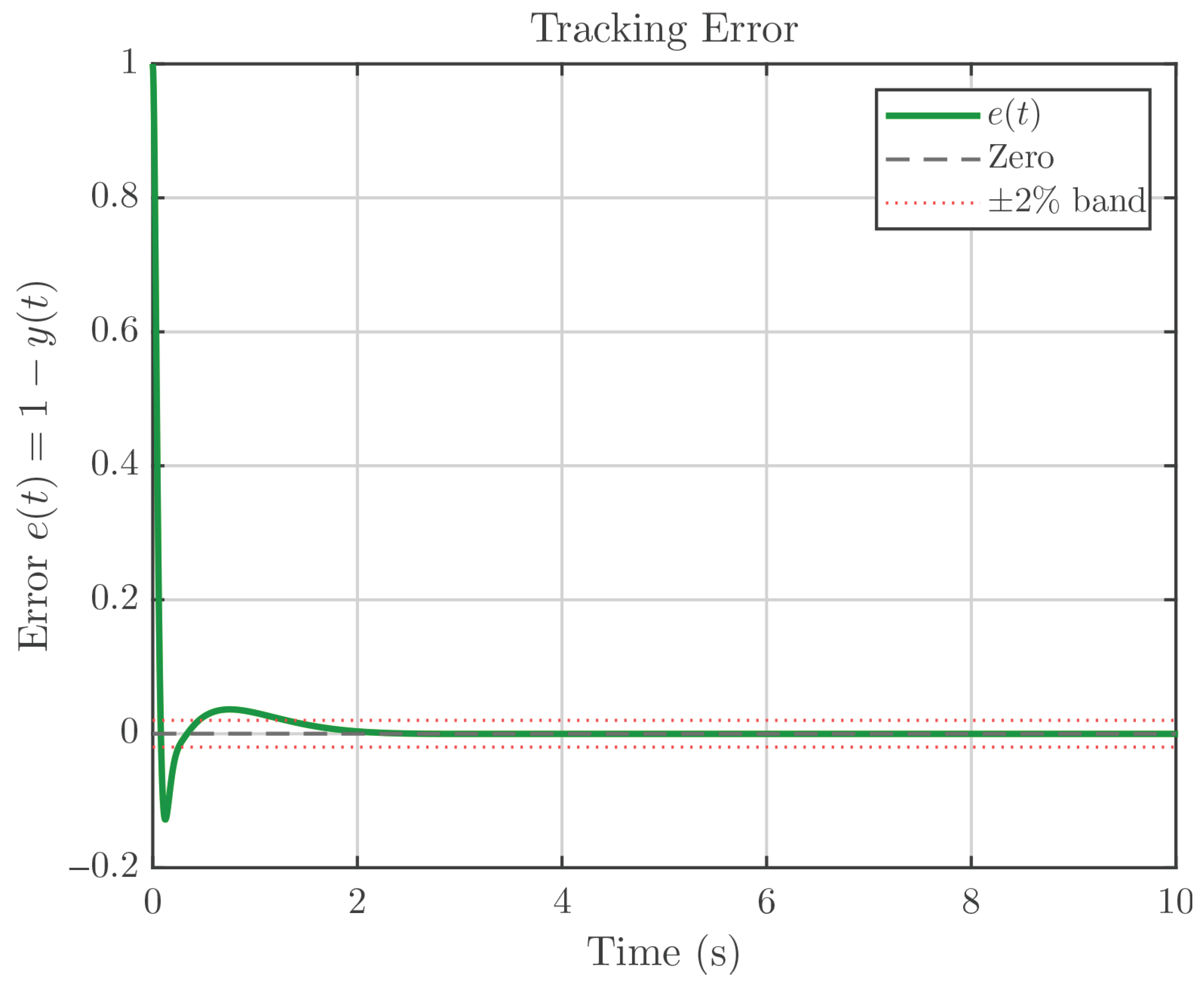
The tracking error in
Figure 10 shows a brief oscillatory transient that decays quickly, confirming the effectiveness of the derivative action in damping the system. The control signal in
Figure 11 exhibits a moderate initial peak followed by a brief negative excursion, before settling to the steady state. The initial control effort is higher than in the first-order case. Nevertheless, it remains bounded and practically feasible for implementation.
The cluster visualization in
Figure 12 shows four distinct clusters in the PID gain space. The optimum (red star) is situated among densely sampled points, indicating successful exploitation, while the spatial spread of all clusters confirms the thorough global exploration.
4.3. Nonlinear Pendulum System
To evaluate performance under nonlinear dynamics and input saturation, a simple pendulum with viscous damping and torque input is considered:
where
is the angular displacement,
m/s
2 is the gravitational constant,
m is the pendulum length,
kg is the mass, and
is the viscous damping coefficient. An input saturation is imposed such that
N·m. The initial condition is
rad (≈34.4°) with
, corresponding to a significant initial displacement from the equilibrium. The simulation is performed using a second-order Runge–Kutta (midpoint) method with step size
s over a horizon of
s.
This system poses several challenges absent in the linear benchmarks: the trigonometric nonlinearity makes the dynamics configuration dependent, the torque saturation introduces hard actuator constraints, and the weak damping () permits oscillatory behavior if the controller is not properly tuned.
The objective is to regulate the pendulum angle to the stable downward equilibrium
using a PID controller with direct saturation enforcement. Unlike the linear systems, no derivative filter is used; instead, the derivative of the error is computed directly from the angular velocity as
. The PID gains are bounded as
The cost function is adapted for the nonlinear setting with four weighted components:
where
penalizes persistent tracking errors;
penalizes large angular deviations;
penalizes control effort;
is a soft saturation penalty that discourages operation near the torque limits.
The weighting coefficients are , , and . The saturation penalty is a distinctive feature of the nonlinear cost function: rather than simply clipping the control signal, it explicitly guides the optimizer away from gain combinations that frequently saturate the actuator.
The algorithm is configured with , initial Sobol points, and the evaluation budget .
The optimal PID gains obtained by SBOC are
yielding a minimum cost of
after 300 function evaluations.
An important finding is that the optimizer converged to , effectively yielding a proportional–derivative (PD) controller. This is physically consistent with the pendulum dynamics: the gravitational restoring torque acts as a natural integral-like mechanism that drives the pendulum toward without requiring explicit integral action. In contrast to the linear systems where integral action was essential to eliminate steady-state error, the nonlinear restoring force ignores it. This demonstrates that the SBOC framework not only optimizes gain magnitudes but also independently discovers the appropriate controller structure dictated by the underlying physics.
Figure 13 presents the convergence history. The objective decreases rapidly during the first 50 evaluations, reaching near-optimal performance, with gradual refinement over the remaining budget. The convergence rate is intermediate between the first-order system (fast) and the second-order system (slow), reflecting the moderate complexity of the nonlinear cost landscape.
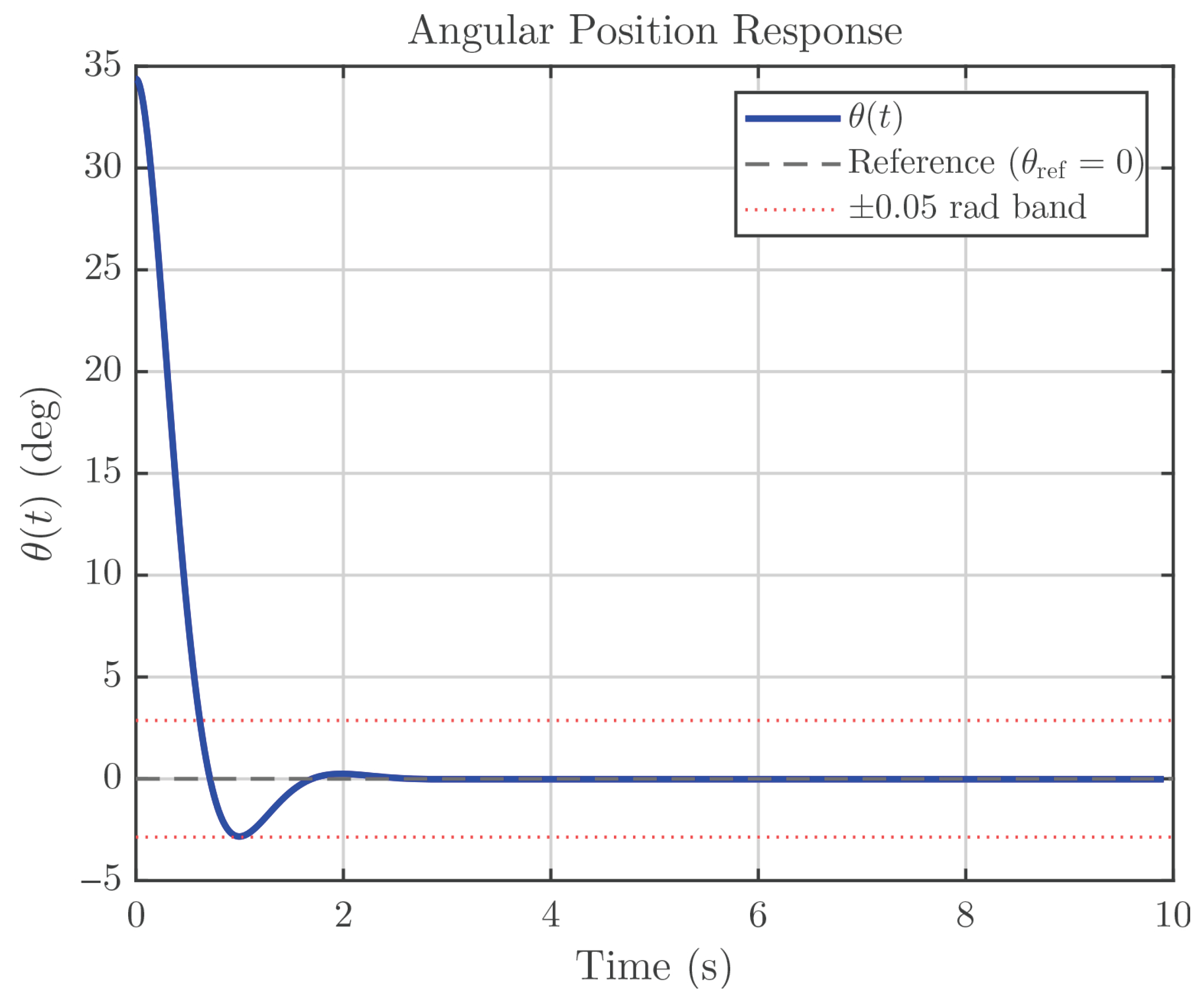
The angular position response is shown in
Figure 14. Starting from
rad, the pendulum converges smoothly to the equilibrium within approximately 0.6 s, entering and remaining within the
rad band. The response exhibits no overshoot past the equilibrium, indicating that the PD controller provides sufficient damping to prevent oscillatory behavior despite the weak inherent damping (
).
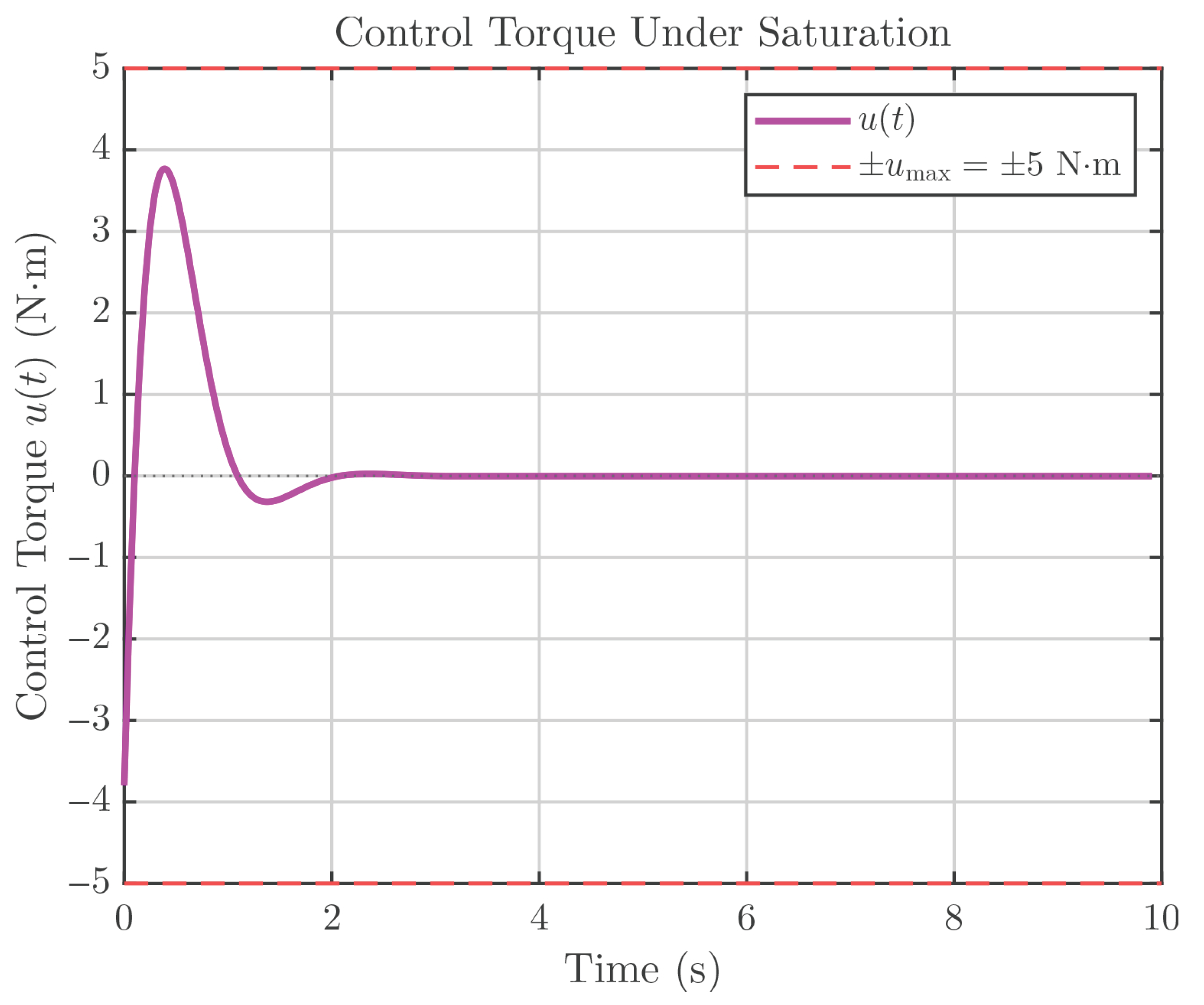
The control torque shown in
Figure 15 remains well within the saturation bounds throughout the entire simulation, with 0% time in saturation. The peak torque is approximately 4 N·m, which is 80% of the
N·m limit. This demonstrates that the soft saturation penalty in the cost function (
40) effectively guided the optimizer toward gain values that avoid actuator limits while still achieving fast convergence.
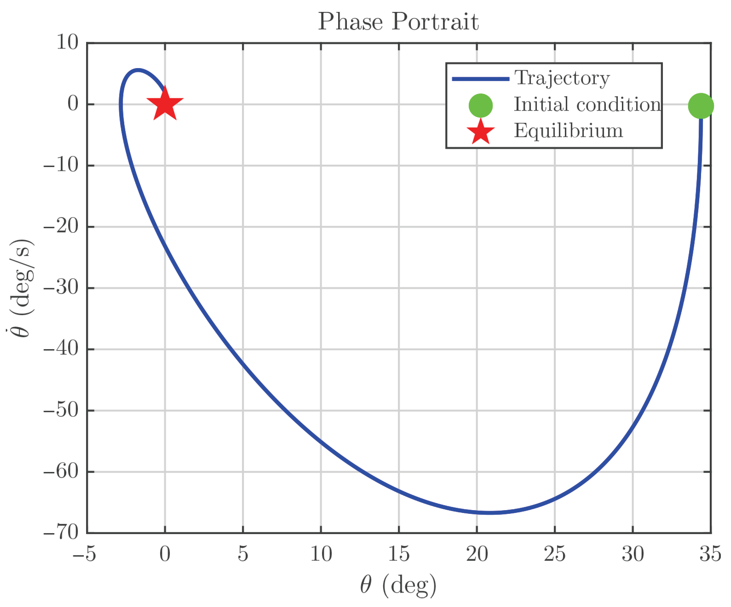
Figure 16 presents the phase portrait (
vs.
), which provides insight into the nonlinear trajectory. The trajectory spirals smoothly from the initial condition
toward the equilibrium at the origin without any limit cycles or oscillatory patterns. This confirms the stability of the controlled nonlinear system and the effectiveness of the derivative action in providing velocity-dependent damping.
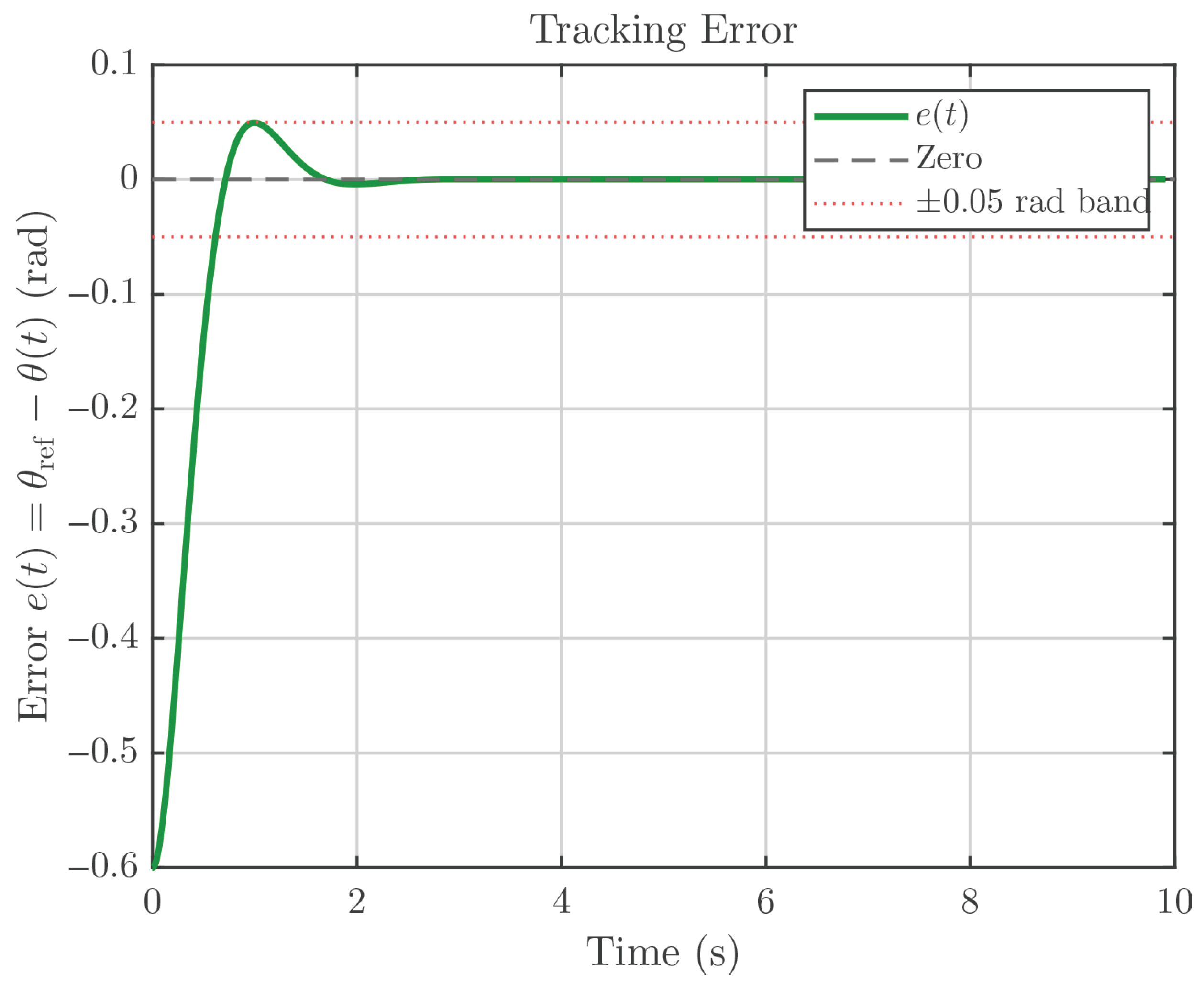
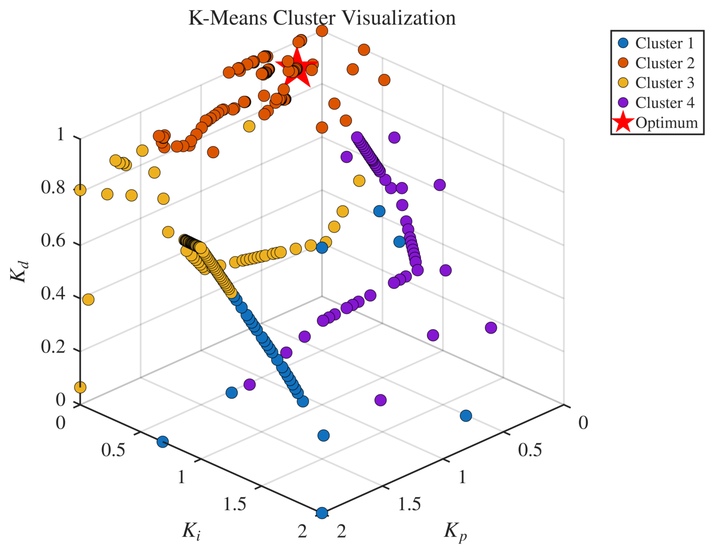
Figure 17 shows the tracking error which eventually tends to zero. Also,
Figure 18 depicts the cluster visualization of the PD values which are divided into four clusters and optimum value is denoted by star which has
.
4.4. Cross-System Comparative Discussion
From the comparative analysis of the first-order, second-order, and nonlinear pendulum case studies, the following observations are made:
- (i)
Physics-aware controller structure selection. The optimizer selected three distinct effective controller structures across the benchmark systems. For the first-order system, the optimal derivative gain was negligible (), indicating that a PI-type controller was sufficient for the monotonic plant dynamics. For the second-order system, a non-negligible derivative gain () was introduced to improve damping and reduce oscillatory behavior, leading to a full PID structure. For the nonlinear pendulum, the optimizer favored a PD-dominant structure, reflecting the importance of velocity-dependent damping in stabilizing the nonlinear motion. This behavior demonstrates that the SBOC framework can implicitly identify the controller complexity required by the plant dynamics without imposing structural constraints a priori.
- (ii)
Role of integral and derivative action. The tuned gains exhibit physically interpretable patterns across systems of increasing complexity. The second-order system required a significantly larger integral gain () than the first-order system (), reflecting the need to maintain zero steady-state error while managing oscillatory transients. In contrast, derivative action was negligible for the first-order system, moderate for the second-order system, and more prominent in the pendulum case, where it contributes to damping under nonlinear motion and weak inherent dissipation.
- (iii)
Cost landscape complexity and convergence behavior. The benchmark results indicate that the optimization landscape becomes progressively more challenging as the system’s complexity increases. The first-order system yielded the lowest objective value and fastest convergence, while the second-order system exhibited a higher optimal cost and slower convergence due to the trade-off between overshoot suppression and settling performance. The nonlinear pendulum further introduced nonconvexity and actuator constraints, resulting in a more structured but still tractable search process.
- (iv)
Transient shaping and damping augmentation. For the second-order system, the SBOC-tuned controller significantly reduced overshoot from the open-loop case and improved damping, demonstrating the effectiveness of optimal gain selection in oscillatory dynamics. For the nonlinear pendulum, the optimized controller achieved stable convergence while keeping the control torque within the imposed saturation bounds, highlighting the ability of the proposed tuning framework to shape the transient response under nonlinear and constrained conditions.
- (v)
Robustness across system classes. An important outcome of this study is that the same SBOC-based tuning framework (with only the cost function and gain bounds adapted to the specific plant) was successfully applied to linear first-order, oscillatory second-order, and nonlinear pendulum dynamics. This consistency supports the generality of the proposed approach and suggests that surrogate-based PID tuning can provide a unified methodology across a broad range of control problems.
From a practitioner’s perspective, the benchmark results yield the following actionable guidelines. (a) For monotonic first-order plants, derivative action provides negligible benefit; engineers may safely fix and reduce the problem to PI tuning. (b) For oscillatory or lightly damped plants, all three PID gains play distinct roles, and the full three-dimensional search is necessary. (c) For nonlinear plants with inherent restoring mechanisms (gravity or spring forces), integral action is often counterproductive and the optimizer will naturally eliminate it. (d) The SBOC surrogate model, once constructed, can be queried at negligible cost to perform sensitivity analysis (for instance, to determine how much a gain perturbation of degrades performance) without additional closed-loop simulations.
5. Application to Type 1 Diabetes Control
Type 1 diabetes is an autoimmune condition in which the insulin secretion from pancreas is absent and therefore it requires exogenous insulin delivery to regulate blood glucose concentrations. The control objective is to maintain glucose within a clinically safe range (70–180 mg/dL) while avoiding two life-threatening complications: hypoglycemia ( mg/dL), which can cause seizures and loss of consciousness, and hyperglycemia ( mg/dL), which over time leads to organ damage. The challenge is compounded by large meal-induced disturbances, slow insulin pharmacokinetics, non-negative insulin constraints (, since insulin cannot be withdrawn), and significant inter-patient variability.
5.1. Bergman Minimal Model
The glucose–insulin dynamics are modeled using the BMM [
22], a widely used three-compartment representation for type 1 diabetes:
where
is the plasma glucose concentration (mg/dL),
is the remote insulin effect (1/min),
is the plasma insulin concentration,
is the exogenous insulin infusion rate, and
is the meal-induced glucose appearance rate. The model parameters are listed in
Table 1.
The meal-induced glucose appearance is modeled using a gamma-shaped absorption profile:
where
g is the carbohydrate content,
min is the meal time,
min is the absorption time constant, and
(mg/dL/min)/g is the glucose appearance scale factor.
5.2. Simulation Scenario
The clinical scenario spans 600 min (10 h) and consists of three phases:
Phase 1 (0–120 min): The initial regulation from an elevated glucose of mg/dL to the target mg/dL.
Phase 2 (120–300 min): A meal challenge; a large 120 g carbohydrate meal at min causes a significant glucose excursion.
Phase 3 (300–600 min): The post-meal recovery and sustained regulation.
The insulin infusion is bounded as units, reflecting the physical constraint that insulin cannot be withdrawn once delivered.
5.3. Safety-Aware Cost Function
The cost function incorporates five clinically motivated components:
where
and
penalize excursions outside the safe zone,
penalizes excessive insulin delivery, and
penalizes rapid insulin changes to ensure smooth delivery profiles. The weighting coefficients are
,
,
,
and
.
The hypoglycemia weight () is two orders of magnitude larger than the hyperglycemia weight (), reflecting the clinical reality that hypoglycemia is an immediate life-threatening emergency, whereas hyperglycemia poses chronic risks. This asymmetric weighting structure is a critical design choice that encodes clinical safety priorities directly into the optimization.
5.4. SBOC Configuration and Results
The PID gains are bounded as
,
, and
, with anti-windup logic on the integrator. The algorithm uses
initial samples and
evaluations. The optimal PID gains obtained by SBOC are
yielding an effective proportional–derivative (PD) controller. The complete results and clinical performance metrics are summarized in
Table 2.
The most striking finding is , meaning the optimizer autonomously eliminated integral action. This decision has a clear clinical rationale: in diabetes management, integral action accumulates insulin over time. Unlike systems where excess control effort can be reversed, exogenous insulin cannot be withdrawn once delivered. The accumulated insulin from integral action creates a risk of delayed hypoglycemia, particularly during the post-meal period when glucose is returning to baseline. The strong hypoglycemia penalty () guided the optimizer to discover that eliminating integral action entirely is the safest strategy.
The derivative gain reached its upper bound, indicating maximal anticipatory action. In diabetes terms, this corresponds to an aggressive correction bolus strategy that responds to the rate of glucose rise rather than the cumulative error. This anticipatory behavior is analogous to the derivative-on-measurement approach used in advanced insulin pump algorithms, where the rate of glucose change (detected by continuous glucose monitors) triggers preemptive insulin adjustments.
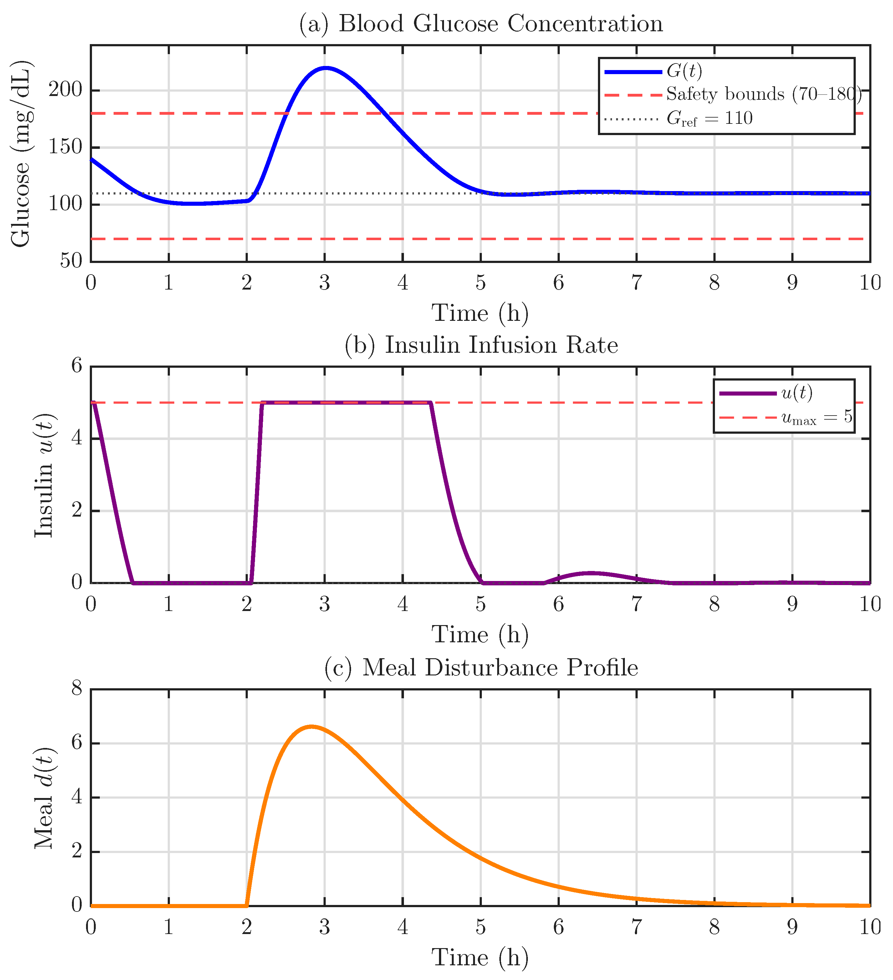
The glucose trajectory under the SBOC-optimized controller is shown in
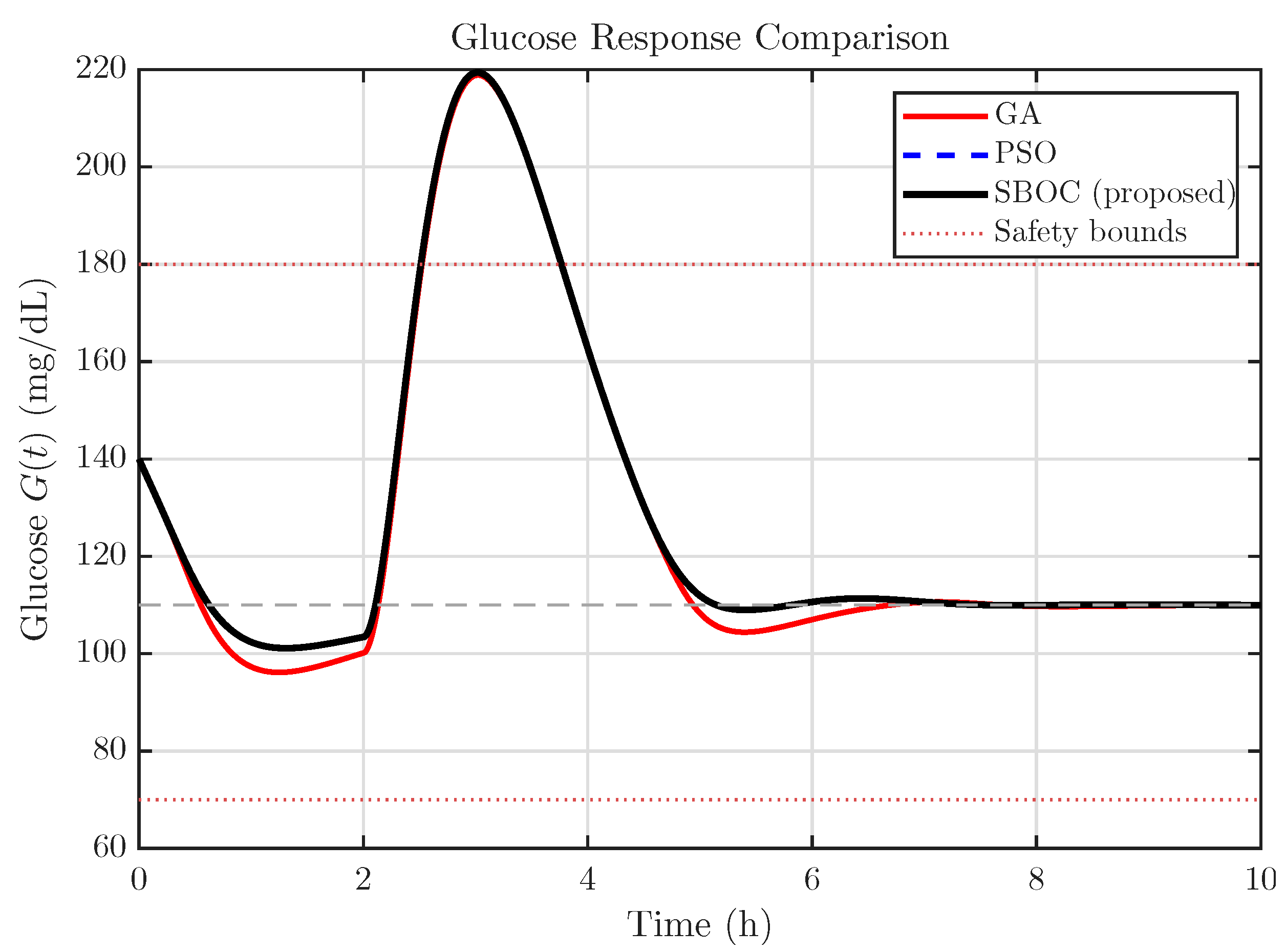
Figure 19. During Phase 1 (0–120 min), glucose settles smoothly from 140 mg/dL to the target of 110 mg/dL. The 120 g meal at
min causes a glucose excursion peaking at 219.4 mg/dL, after which the controller drives glucose back into the safe zone. Critically, glucose remains above 101.1 mg/dL throughout the entire 10 h simulation, with zero hypoglycemic events.
The insulin delivery profile in
Figure 19b shows that the controller responds aggressively to the meal-induced glucose rise, reaching the maximum allowable rate of five units during the peak disturbance period. The insulin delivery is smooth and physiologically realistic, with no chattering or oscillatory behavior—a direct consequence of the smoothness penalty
in the cost function.
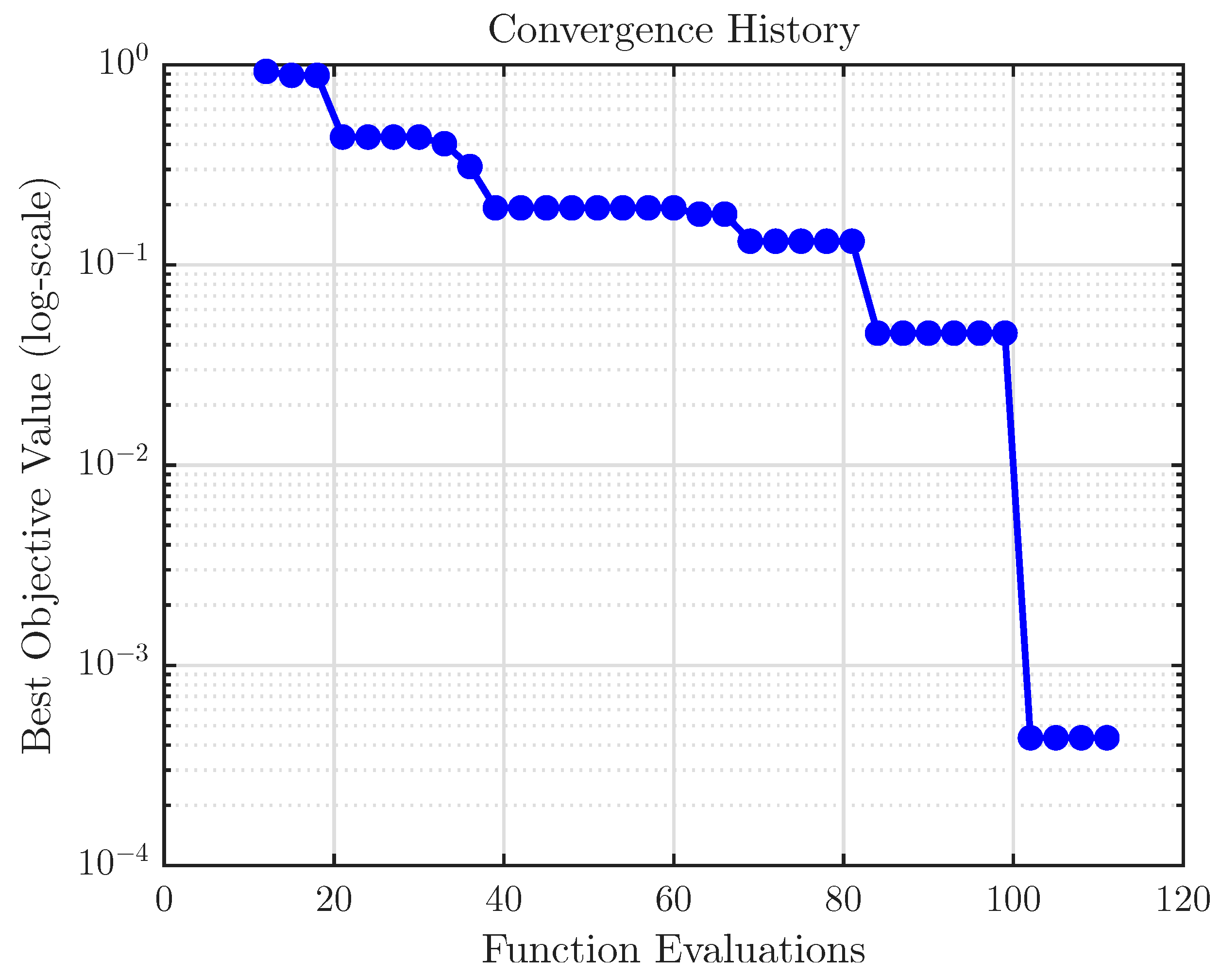
Figure 20 shows the convergence history. The optimizer identifies the low-
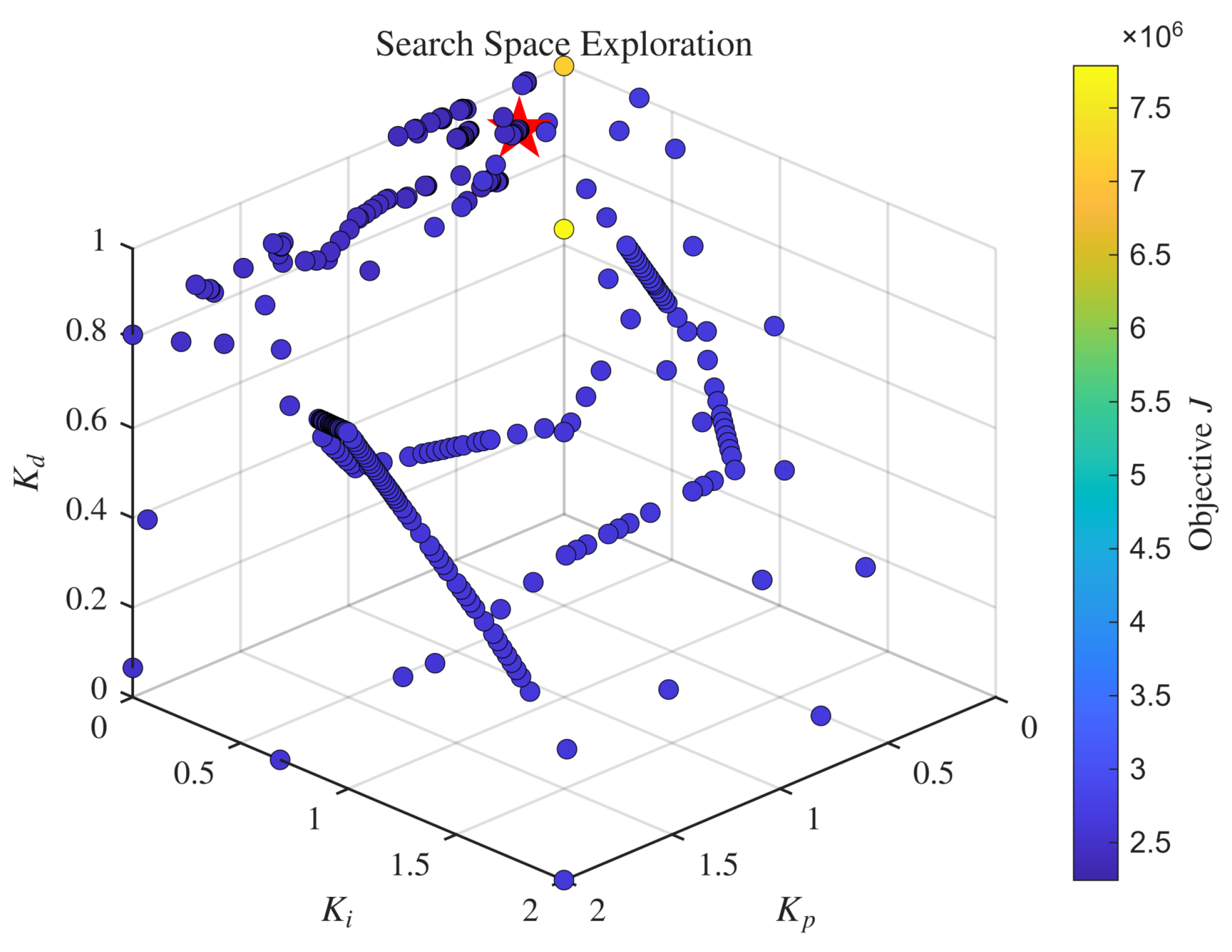
region quickly, with the cost stabilizing after approximately 100 evaluations. The late-stage iterations primarily add only exploratory points (with most surrogate minimum and exploitation points skipped as “too close”), confirming the convergence to a well-defined optimum. Further, the 3D distribution of PID values and their cluster visualization are shown in
Figure 21 and
Figure 22 which reveal that
.
5.5. Discussion
In a safety-critical context, the BMM application demonstrates several important capabilities of the proposed framework:
- (i)
Safety-first optimization. The asymmetric penalty structure () successfully encoded clinical priorities, resulting in zero hypoglycemic events. This demonstrates that domain-specific safety requirements can be naturally incorporated into the SBOC cost function without requiring additional constraint-handling mechanisms.
- (ii)
Clinically interpretable controller structure. The elimination of integral action () is consistent with modern diabetes management practice, where “insulin stacking” (the accumulation of active insulin from overlapping boluses) is a recognized cause of iatrogenic hypoglycemia. The optimizer independently discovered this clinical insight from the mathematical structure of the problem.
- (iii)
Derivative-dominant control. The maximal derivative gain (, at the upper bound) suggests that anticipatory control based on the rate of glucose change is the most effective strategy for meal disturbance rejection. This finding aligns with the clinical motivation behind continuous glucose monitoring systems, which provide real-time rate-of-change information.
- (iv)
Controller structure consistency. The PD structure identified for the BMM echoes the pendulum result ( in both cases), but for fundamentally different reasons. In the pendulum, gravity provides natural restoring action; in diabetes, the non-reversibility of insulin delivery makes integral action dangerous. This demonstrates that the SBOC framework can arrive at the correct controller structure regardless of the underlying physical or physiological mechanism.
6. Comparison with Metaheuristic Methods
To comprehend the competitiveness of the SBOC-based tuning approach, we compare it against two widely used population-based metaheuristic methods: GA [
32] and PSO [
33]. The comparison is conducted on the two nonlinear systems, that is, the pendulum and the glucose regulation problem, where the optimization landscape is more challenging. Ten independent runs per method are performed, each with the same evaluation budget of 300 function evaluations (
), identical cost functions, and identical gain bounds.
For GA, MATLAB 2025b’s ga() function is used with a population size of 30, crossover fraction of 0.8, two elite individuals, and adaptive feasible mutation. For PSO, MATLAB’s particleswarm() is used with a swarm size of 30, social and cognitive weights of 1.49, and inertia in . Both methods terminate after generations/iterations. Each run uses a distinct random seed for reproducibility.
6.1. Pendulum Results
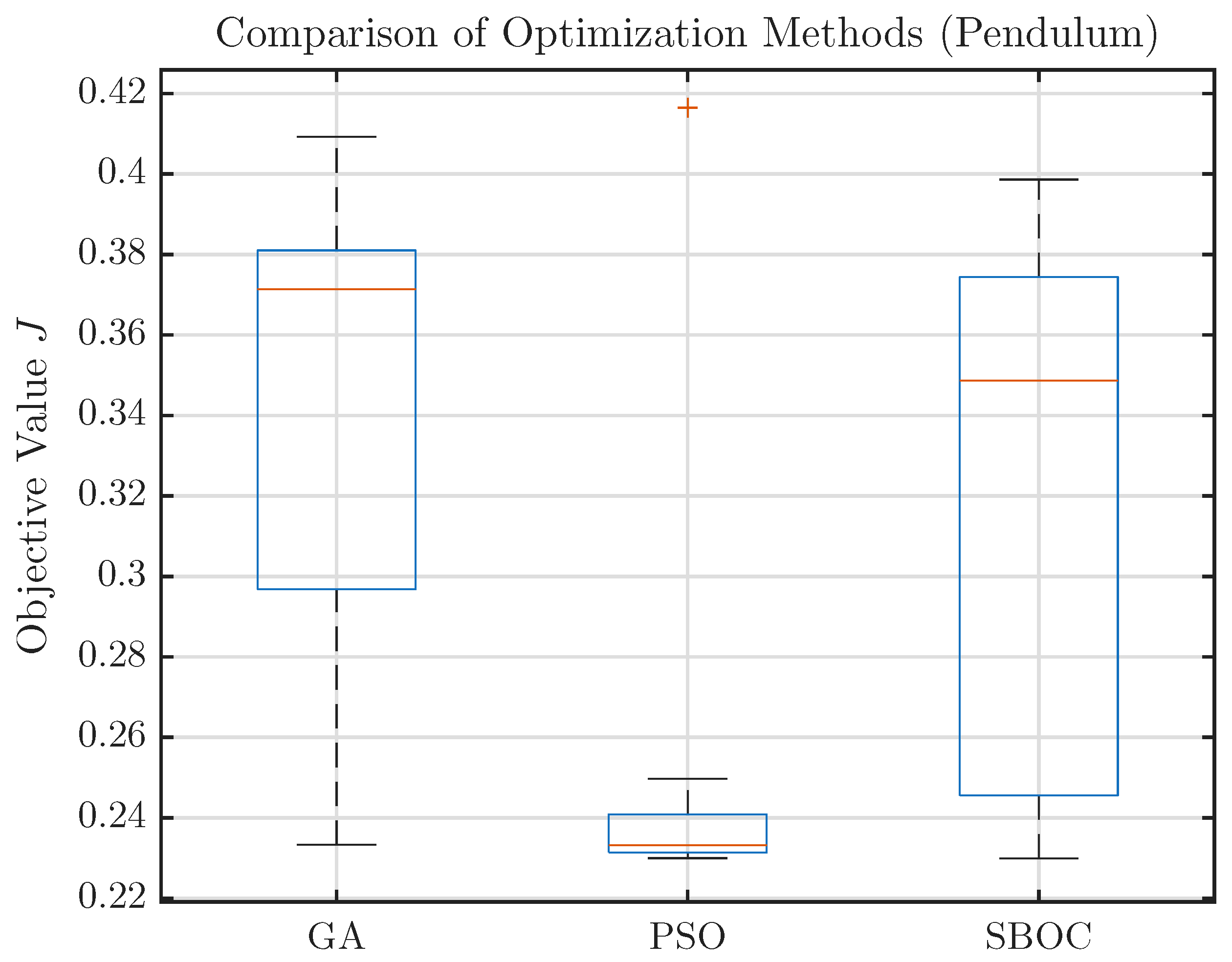
Table 3 summarizes the statistical results for the nonlinear pendulum. All three methods converge to essentially the same optimal PD controller structure (
), with best-case objective values differing by less than 1.5%. SBOC achieves the lowest single run optimum (
), marginally outperforming PSO (
) and GA (
) (also see
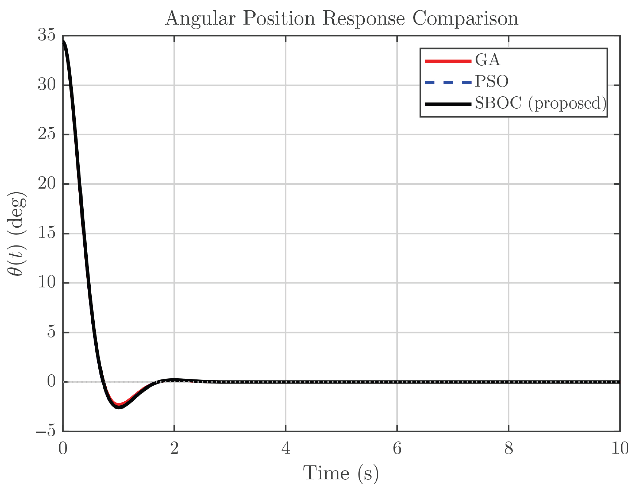
Figure 23). However, PSO exhibits superior run-to-run consistency, with the lowest mean and standard deviation across ten runs. The angular response trajectories under the best controller from each method are visually indistinguishable (
Figure 24), confirming that all three methods identify the same control behavior.
6.2. BMM Results
Table 4 presents the comparison for the type 1 diabetes (T1D) glucose regulation problem, and
Table 5 reports the clinical performance of the best controller from each method.
The results reveal several important observations. First, all three methods independently discover the PD controller structure (), providing strong cross-validation of the finding that integral action is detrimental for this safety-critical application. SBOC and PSO converge to nearly identical optimal gains (, ), yielding clinically equivalent performance with zero hypoglycemia in all cases.
Second, PSO demonstrates the highest run-to-run consistency for the BMM problem, with a remarkably low standard deviation () compared to SBOC () and GA (). This is attributed to the narrow, well-defined structure of the BMM cost landscape: the optimal region lies along the boundary face with at its upper bound, leaving effectively a one-dimensional search over . In such a reduced dimensionality setting, the swarm dynamics of PSO are highly efficient at converging across multiple runs.
Third, SBOC exhibits higher variance because its exploration–exploitation strategy invests a portion of evaluations in global surrogate construction, occasionally sampling in suboptimal regions. While this exploration is beneficial in higher-dimensional or multi-modal landscapes, it reduces the consistency in the low-dimensional () problems studied here.
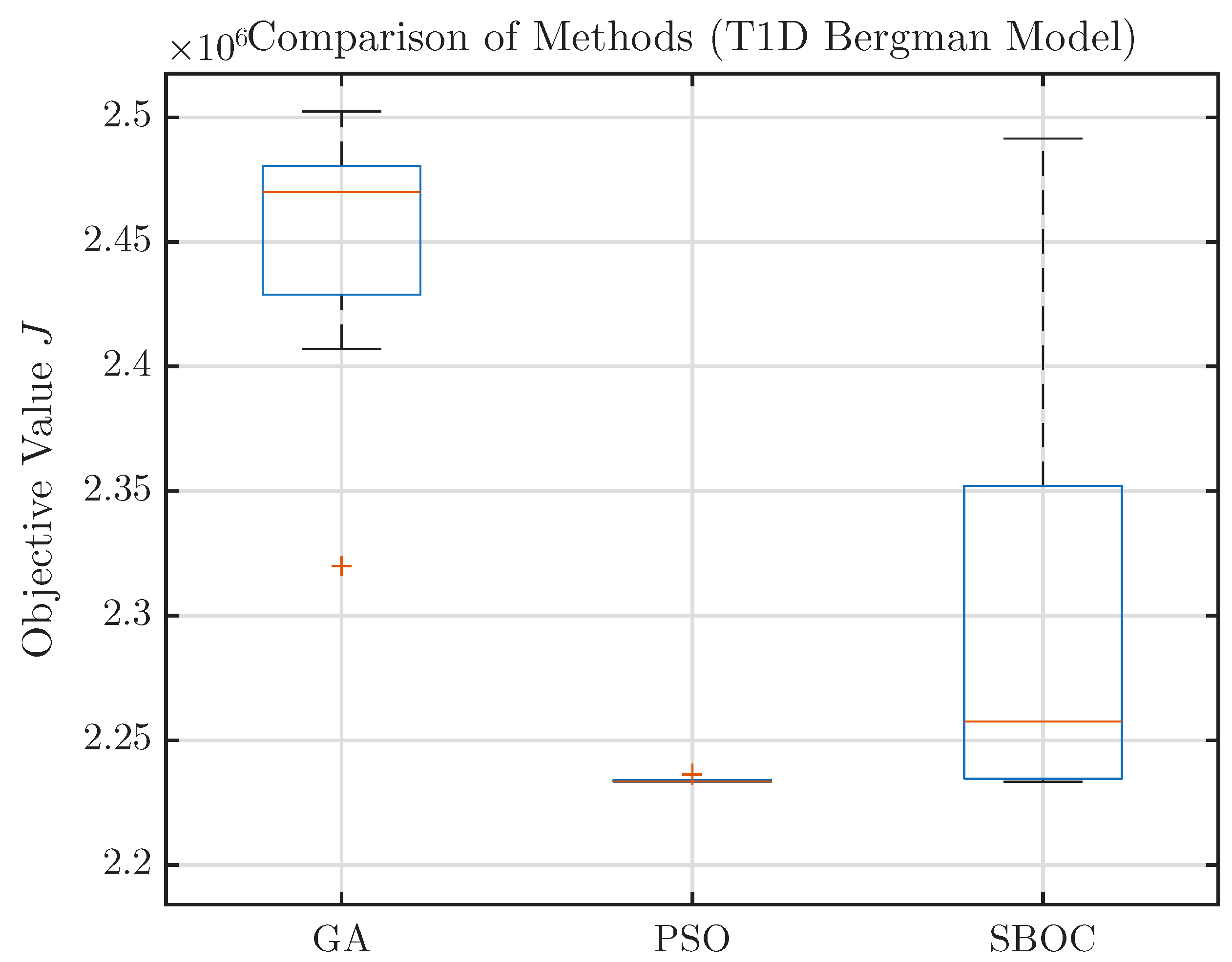
The comparative performance of the three optimization methods on the BMM problem is further illustrated in
Figure 25 and
Figure 26.
Figure 25 shows the glucose trajectories corresponding to the best controller obtained by each method, indicating broadly similar regulation characteristics with slight differences in postprandial excursion and recovery behavior in GA.
Figure 26 presents the distribution of the objective values across ten independent runs, providing a clearer view of the relative robustness and run-to-run consistency of GA, PSO, and SBOC.
6.3. Discussion of Comparative Results
The following are the key insights from this comparative study:
- (i)
Solution quality. SBOC achieves best-case solution quality that is competitive with, or marginally better than, both GA and PSO. All three methods converge to the same controller structures, providing an independent cross-validation of the physics-aware gains identified by SBOC.
- (ii)
Consistency vs. exploration. PSO exhibits superior run-to-run consistency for these low-dimensional () problems. This is expected with only three parameters; a swarm of 30 particles provides dense coverage of the search space, and population-based consensus quickly narrows the search. SBOC, by design, allocates evaluations to build a global surrogate model, which reduces its convergence consistency for small N but provides landscape information that is not available from population-based methods.
- (iii)
Surrogate model as a secondary output. Unlike GA and PSO, which return only the best solution, SBOC constructs a global RBF surrogate that maps the entire gain space to the cost function. This model can be reused for sensitivity analysis, constraint exploration, or warm-starting subsequent optimizations without additional simulation cost.
- (iv)
Clinical safety. All three methods achieve zero hypoglycemia across all 30 BMM runs (ten per method), confirming that the asymmetric penalty structure () robustly encodes clinical safety regardless of the optimization algorithm employed.
- (v)
Scaling considerations. For the low-dimensional problems in this study, population-based methods are highly effective. SBOC’s primary advantage—sample efficiency through surrogate guidance—is expected to become more pronounced in higher-dimensional parameter spaces (e.g., cascaded PID and multi-loop control) where population-based methods require substantially more evaluations to achieve comparable coverage.
- (vi)
Stability and optimality. The current framework does not provide formal stability guarantees (e.g., Lyapunov-based proofs) for the tuned parameters. The stability is enforced implicitly: unstable closed-loop configurations produce unbounded simulation outputs, which are assigned the penalty , effectively excluding them from the feasible set. The ITAE cost further penalizes marginally stable or poorly damped responses. Regarding optimality, the independent convergence of GA, PSO, and SBOC to the same controller structures and nearly identical gain values provides strong empirical evidence of near-optimality. Furthermore, the discovered controller structures (PI, PID, and PD) are robust to variations in the weighting coefficients: in unreported experiments, varying from 20 to 100 and from 0.001 to 0.1 consistently yielded the same structural outcome (e.g., for the pendulum), with only the gain magnitudes shifting. Post-optimization Lyapunov analysis or robust stability margin computation could complement the simulation-based tuning and is identified as future work.
- (vii)
Breakeven analysis. In terms of wall clock time, GA and PSO are faster for the benchmarks studied (0.08–0.33 s vs. 27–35 s per SBOC run), because the per-evaluation simulation cost – s is small relative to the SBOC overhead of surrogate construction and multi-start minimization. However, when is large (e.g., s, as in high-fidelity CFD or multi-patient virtual trials), the surrogate overhead becomes negligible relative to the total simulation cost, and SBOC’s sample efficiency translates directly into wall clock time savings. The breakeven point can be estimated as s per evaluation for the current implementation, above which SBOC becomes time-competitive with population-based methods at equal evaluation budgets.
As far as optimality is concerned, since the cost landscapes studied here are nonconvex, global optimality cannot be formally guaranteed by any of the three methods. However, the independent convergence of GA, PSO, and SBOC to the same controller structures and nearly identical gain values provides strong empirical evidence of near optimality. The probability that three fundamentally different optimization paradigms, that is, evolutionary, swarm-based, and surrogate-guided, would independently converge to the same suboptimal point is low in a multi-modal landscape. This cross-validation is particularly meaningful for the automatic structure selection finding, where all three methods independently eliminate
for the pendulum and diabetes problems. For low-dimensional problems (
), model-free methods such as iterative feedback tuning [
15] and Bayesian optimization [
18] offer competitive alternatives. The distinguishing advantage of SBOC lies in the construction of a global RBF surrogate as a reusable secondary output, which encodes the full cost landscape and can support important tasks such as sensitivity analysis, robustness certification, or the warm-starting of related tuning problems.
7. Conclusions and Future Work
This paper presented a SBOC framework for the tuning of PID controllers for linear, nonlinear, and physiological dynamical systems. The proposed approach was motivated by the practical difficulty of PID tuning when the closed-loop performance must be evaluated through repeated simulation and when the underlying cost landscape is nonconvex. By combining surrogate-guided search with simulation-based objective evaluation, the framework provides a unified methodology for controller tuning without requiring explicit analytical tuning rules.
The effectiveness of the proposed approach was demonstrated on four case studies comprising first- and second-order LTI systems, a nonlinear pendulum with actuator saturation, and blood glucose regulation in type 1 diabetes. Across these systems, the optimizer identified controller gains that were physically meaningful and dynamically appropriate for the corresponding plant. In particular, the results showed that the effective controller structure varied naturally with systems’ characteristics, yielding PI-like behavior for the first-order plant, full PID action for the second-order system, and PD-dominant solutions for the nonlinear pendulum and diabetes model. The framework also demonstrated the ability to incorporate safety-oriented objectives, especially in the diabetes application, where glucose was maintained within the clinically acceptable range for most of the simulation horizon without hypoglycemic events.
The present work is limited to low-dimensional PID tuning problems, deterministic simulations, and representative operating scenarios. Several directions for future work are identified based on the current findings, which are as follows:
- (i)
Robustness under uncertainty. The current framework assumes deterministic plant parameters and noise-free measurements. Incorporating additive sensor noise, process disturbances, and parametric uncertainty through Monte Carlo analysis across randomized patient populations in the diabetes application would help in investigating the practical robustness of the optimized PID gains. This may further reveal the need for robust or stochastic cost function formulations. If measurement noise is added to the simulation, each evaluation of becomes stochastic. In that case, a regression-based RBF (with a regularization parameter) instead of exact interpolation, or averaging each evaluation over multiple noise realizations, would be required to prevent overfitting to individual noise instances. These noise-robust surrogate formulations represent an active research direction in surrogate-based optimization.
- (ii)
Stochastic and multi-scenario disturbance rejection. The current framework handles deterministic disturbances. For stochastic disturbances, two compatible extensions exist without algorithmic changes to SBOC: (a) an expected value formulation that evaluates each candidate by averaging over M Monte Carlo disturbance realizations, or (b) a worst-case formulation that uses over a set of disturbance scenarios. Both approaches only modify the cost function wrapper.
- (iii)
Formal statistical validation. Formal statistical hypothesis testing (e.g., the Wilcoxon rank sum test or Friedman test) should be applied to the distributions of objective values across multiple optimization runs. This would provide rigorous evidence for performance comparisons beyond the descriptive statistics (mean and standard deviation) currently reported, and would strengthen the empirical assessment of competing methods.
- (iv)
RBF hyperparameter sensitivity. A systematic sensitivity study on the RBF shape parameter and its cross-validation strategy would provide insight into the algorithmic robustness of SBOC. The current implementation selects automatically via 5-fold cross-validation at each iteration. Comparing fixed versus adaptive selection strategies and their impact on the convergence speed and solution quality is of particular interest.
- (v)
Multi-objective and Pareto front analysis. The aggregated scalar cost function used here could be decomposed into its constituent objectives, enabling a multi-objective analysis. Generating Pareto fronts between the competing criteria (for example, the time in range versus the control effort, or the tracking speed versus the hypoglycemia risk) would provide clinicians and engineers with a set of non-dominated controller options. These options help in prioritizing patient-specific or application-specific selections.
- (vi)
Scalability to higher-dimensional architectures. The scalability of the SBOC framework to higher-dimensional parameter spaces is an important open question. The current study addresses decision variables. The computational cost per SBOC iteration scales as for RBF matrix inversion, which remains tractable up to approximately –2000 sample points, corresponding to problems with –20 dimensions. For example, a fractional-order PID architecture (: ) would require –1000, which remains tractable. Cascaded PID or multi-loop designs (–9) would need –2000 evaluations. Beyond –20, strategies such as dimension reduction via sensitivity screening, local RBF surrogates instead of a single global model, and partial separability exploitation when gain blocks are decoupled should be investigated. Scaling beyond dimensions remains an open challenge for all RBF-based surrogate methods.
- (vii)
Formal stability verification. The current framework handles stability implicitly. The unstable closed-loop configurations produce unbounded simulation outputs, which are assigned the penalty , effectively excluding them from the feasible set, and the ITAE cost further penalizes marginally stable or poorly damped responses. However, formal stability certificates (e.g., Lyapunov-based analysis, small-gain theorems, or robust stability margin computation) are not provided. This limitation is shared with all simulation-based metaheuristic tuning approaches (GA, PSO, and DE). Post-optimization Lyapunov analysis or robust stability margin computation could complement the SBOC tuning and is identified as important future work.
- (viii)
Validation on challenging plant classes. Future benchmarks should include delay-dominant systems (e.g., ), non-minimum phase (NMP) plants, and open-loop unstable systems. While the SBOC framework is agnostic to plant type, dead-time systems produce more challenging cost landscapes with sharper optima, and NMP plants impose inherent bandwidth limitations that the ITAE cost will naturally reflect. For open-loop unstable plants, the optimizer would discover minimum stabilizing gain thresholds through the penalty mechanism. Adjusting the gain bounds appropriately for each plant class is a practical prerequisite.
- (ix)
Online adaptation and MIMO extensions. The current framework is an offline, design time tool. Limitations preventing direct online use include the computational overhead of RBF surrogate training and multi-start minimization (0.1–0.5 s per iteration), as well as the requirement that each candidate gain be evaluated through a complete simulation or physical trial lasting at least one settling period, and the safety risk of exploring untested gains on a physical plant. Feasible online adaptation strategies include using the pre-built surrogate as a warm start and restricting exploration to a safe neighborhood of the current operating point. Extension to MIMO systems with M PID loops would expand the decision vector to ; the surrogate would approximate the aggregate MIMO cost, which inherently captures cross-coupling through the full closed-loop simulation. Decentralized tuning strategies exploiting structural sparsity could reduce the effective dimensionality for large-scale systems.
- (x)
Hybrid reinforcement learning (RL) directions. An interesting future direction is a two-stage SBOC–RL hybrid, in which SBOC performs offline optimization to identify near-optimal PID gains and construct a global surrogate model, and an RL agent subsequently uses these gains as the initialization for online fine-tuning as the plant drifts [
34]. The SBOC surrogate could serve as a value function approximation to accelerate RL training, and its inter-cluster gap identification could inform RL exploration policies in the parameter space. A supervisory RL layer that monitors the discrepancy between the surrogate’s predicted cost and the actual closed-loop cost would be particularly relevant for the diabetes application. In such applications, a supervisor could revert to basal-only insulin delivery if the controller’s predictions diverge significantly from measured glucose values. These hybrid directions, including the use of the surrogate as a world model or digital twin to bridge the simulation-to-real gap, are identified as compelling avenues for future investigation.