1. Introduction
Complex parts refer to a category of mechanical parts characterized by intricate geometric profiles or sophisticated spatial architectures, designed to achieve advanced or specialized functionalities [
1,
2,
3]. Complex parts are widely employed in engineering fields such as aerospace, transportation, energy, nuclear, and microelectronics, including complex-curved parts like aero-engine turbines, marine propellers, and steam turbine blades, as well as complex-structured parts such as automotive engine blocks and marine crankshafts [
4,
5,
6]. With the ongoing pursuit of high efficiency, precision, quality, and extreme functionality in modern high-end manufacturing, mechanical systems and structures are trending toward ultra-high speed, high acceleration, heavy loading, lightweighting, multi-degree-of-freedom designs, and high reliability. These trends will significantly expand the development and application of complex parts.
As core components of assemblies or machinery, complex parts must undergo comprehensive geometric inspection to ensure they have the intended functionality. Current 3D shape inspection methods for mechanical parts primarily include contact and non-contact techniques. Among these, laser-based non-contact shape inspection offers advantages such as nondestructive operation, high efficiency, considerable accuracy, good environmental adaptability, and low equipment costs, making it a major development trend in part shape inspection [
7]. Consequently, numerous researchers have conducted extensive studies on laser non-contact 3D shape inspection methods.
Yao Wang et al. [
8] established a 3D shape measurement model using multiple parallel line lasers. In this model, the spatial distribution of laser lines is determined by object surface features, while a motor-driven scanning mechanism acquires additional contour data to enhance lateral resolution. Guowei Yang et al. [
9] employed a MEMS scanning module to project temporally modulated line laser stripes into the measurement space, generating high-resolution fringe patterns for improved measurement precision. This approach effectively captures microscopic height variations in the measured parts. Qiucheng Sun et al. [
10] proposed a multi-line structured light method that integrates single-line and triple-line lasers. With no precision slide rails or displacement measurement devices, the system performs real-time scanning plane calibration during measurement by leveraging intersections between the mobile single-line laser and fixed triple-line lasers. This technique overcomes challenges in acquiring specific angular and positional data. Chuanwei Yao et al. [
11] developed an omnidirectional laser scanning system comprising a rotational laser scanner and paired planar mirrors. With mirror assistance, projected line lasers illuminate samples from all angles in a single scanning sequence, while cameras capture 3D data from optimized viewpoints. This rotary scanning strategy enables high-efficiency, large-scale 3D inspection. Ding Ke et al. [
12] introduced a laser scanning technique for large structural surface profiling. Using a line laser source as the projection unit, the system scans the surface at controlled angular velocities while capturing images with fixed imaging units. An image fusion strategy constructs fringe patterns with constant phase shifts. When applied to wind turbine blade inspection, this technique has achieved promising results.
For complex parts, acquiring complete surface topography data requires the laser sensor to move through space while continuously adjusting its pose to adapt to surface geometry variations. Since laser sensors inherently lack spatial positioning capability, they are typically mounted on positioning platforms when performing 3D inspection tasks. Researchers have consequently investigated laser-based 3D inspection systems integrated with positioning platforms.
Chao B et al. [
13] established a non-contact laser 3D measurement system using a traditional Coordinate Measuring Machine (CMM). By replacing the tactile probe with a laser sensor, the system drives 3D scanning via the CMM’s Z-axis movement. However, CMMs are relatively expensive, and the limited motion freedom of the Z-axis may pose challenges for comprehensive inspection of complex parts. Xie et al. [
14] integrated a line laser sensor with an Articulated Arm Coordinate Measuring Machine (AACMM) and proposed a flexible scanning method. Experiments on complex parts demonstrated the system’s adaptability, enabling measurements from arbitrary orientations. Nevertheless, as the AACMM is a passive device, it cannot achieve automated inspection.
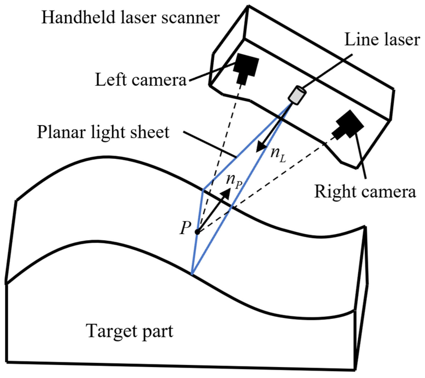
With advances in machine vision technology, handheld laser scanners have emerged [
15,
16,
17]. These scanners require no positioning platforms during inspection but only need to properly arrange some fiducial markers on the part surface and surrounding areas. During the scanning process, the system continuously aligns and stitches acquired image data based on these markers, thereby reconstructing comprehensive 3D topographical data of the measured component.
Handheld laser scanners are widely used in 3D shape inspection due to their portability, high speed, and relatively high accuracy. However, as the scanning process is manually controlled, it is difficult to consistently maintain optimal measurement poses, distances, and velocities throughout the inspection. This prevents the sensor from achieving its full performance potential. Furthermore, for batches of identical parts, manual scanning cannot ensure consistent scanning paths across different parts, leading to variability in inspection results. In addition, manual operation is susceptible to individual differences such as work experience, skill level, and physical fatigue, resulting in issues with unstable work efficiency and inspection quality.
With the advancement of robotics technology, many researchers have introduced robots into the field of shape inspection. Al Khawli et al. [
18] integrated a laser profile sensor with a 6-DOF robot to automatically inspect simple geometric features such as hole diameter and spacing. Mineo et al. [
19] automated non-destructive testing by mounting a thermographic camera on a 6-axis robot, which positions the sensor to acquire thermal images from optimal viewpoints, enabling defect detection in large, geometrically complex components. Ajman et al. [
20] designed a specialized robotic arm for automated non-destructive testing of curved aerospace surfaces. By maintaining optimal sensor orientation and standoff distance during scanning, the robot improves inspection accuracy while enhancing technician safety through automation of a previously manual and hazardous process. Asif et al. [
21] introduced a twin-robot system for 3D X-ray imaging, where collaborative robots maneuver imaging equipment in tandem to enable comprehensive scans with enhanced diagnostic accuracy and efficiency over traditional methods. Wu et al. [
22] equipped a 7-DOF arm with integrated ultrasonic and vision modules for automated fastener hole inspection, combining visual localization with real-time ultrasound feedback to achieve precise probe alignment and consistent coupling. Liu et al. [
23] developed an automated inspection system for aeroengine cooling holes that integrates a robotic arm, an infrared camera, and deep learning techniques, where the robotic arm captures infrared sequences to construct a comprehensive dataset.
Path planning is often a critical technique in robot-assisted inspection. To address this, Zhao et al. [
24] proposed a stepwise optimization framework for multi-robot coverage path planning on large free-form surfaces, ensuring full surface coverage while balancing inspection efficiency and scanning accuracy. Chen and Jia et al. [
25,
26] developed a robotic inspection system for free-form surface parts by integrating an industrial robot with a line laser sensor and a tracker. For measurement path planning, they employed the geometric length of the scanning path and the amplitude variation of the Euler angles as the objective function. Chen et al. [
27] proposed a particle swarm optimization (PSO)-based path generation method for robotic line scanners to minimize inspection time in automated surface defect detection of 3C free-form objects.
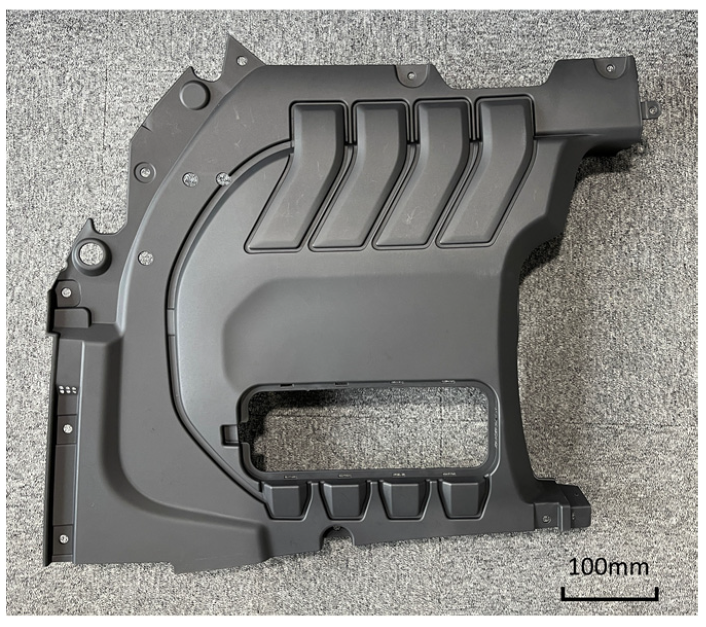
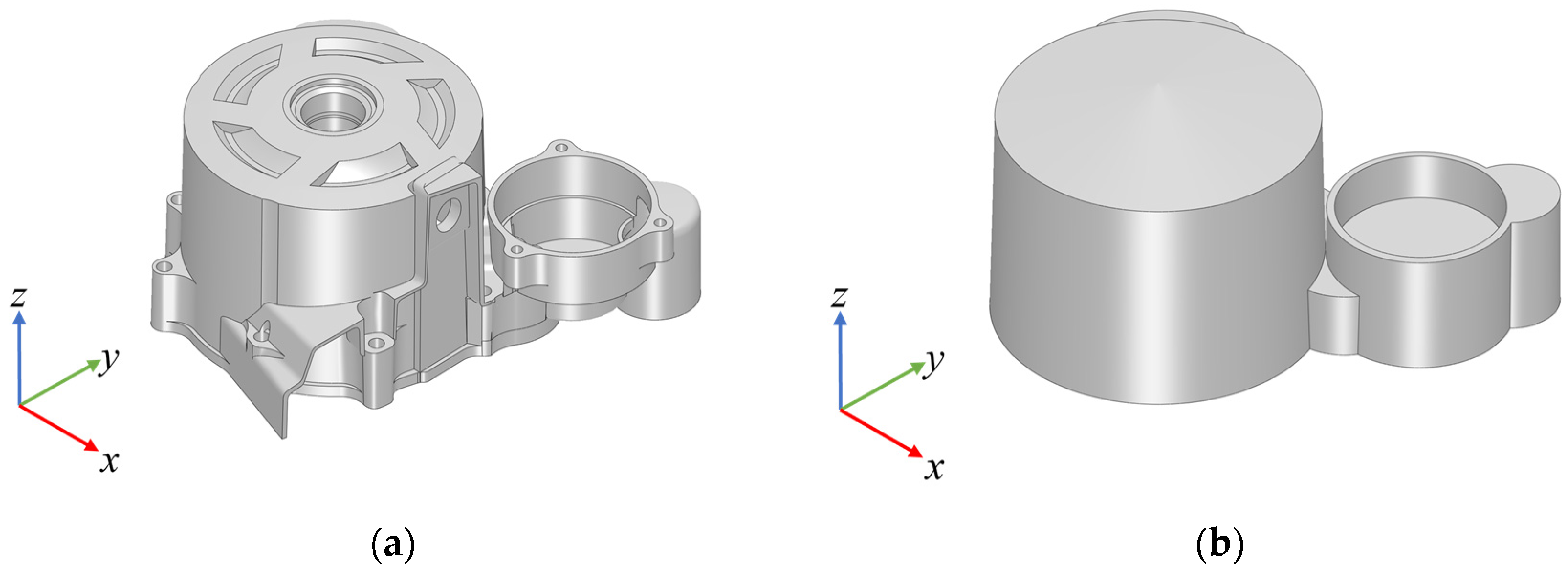
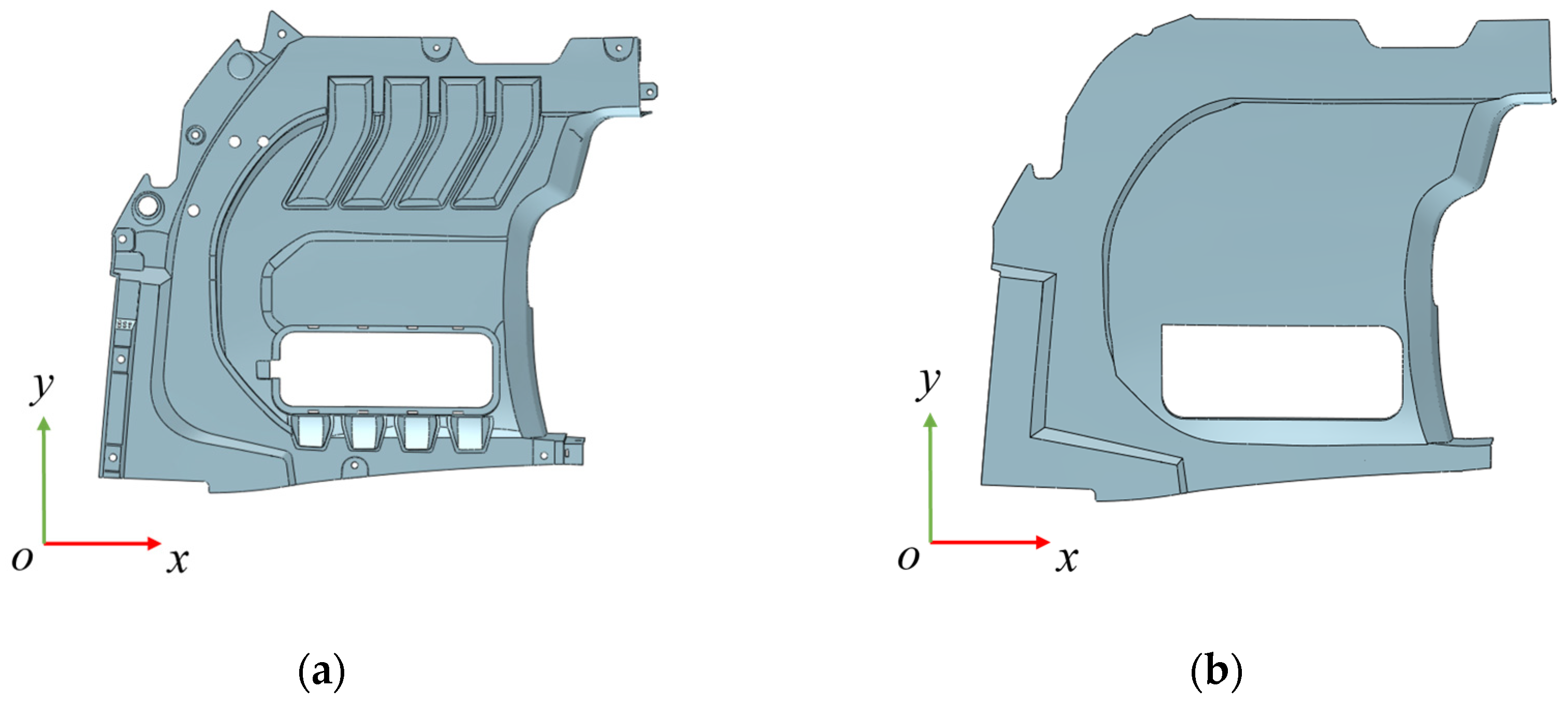
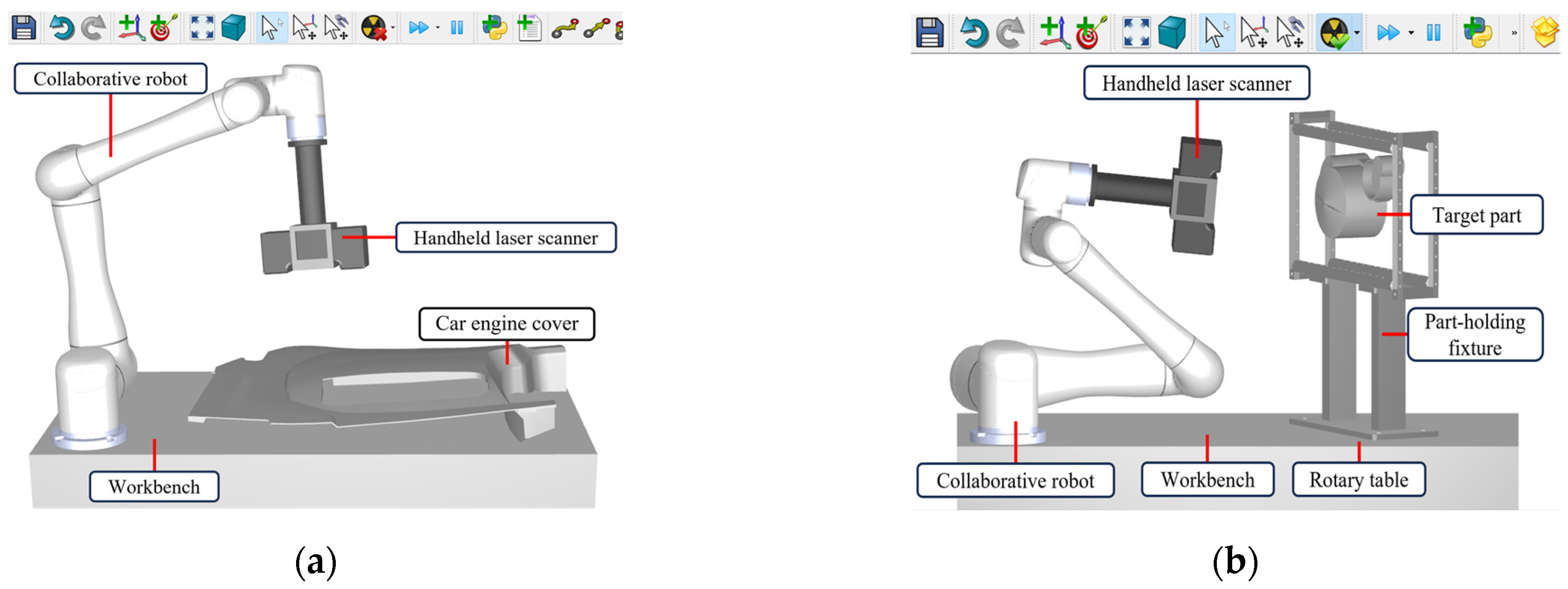
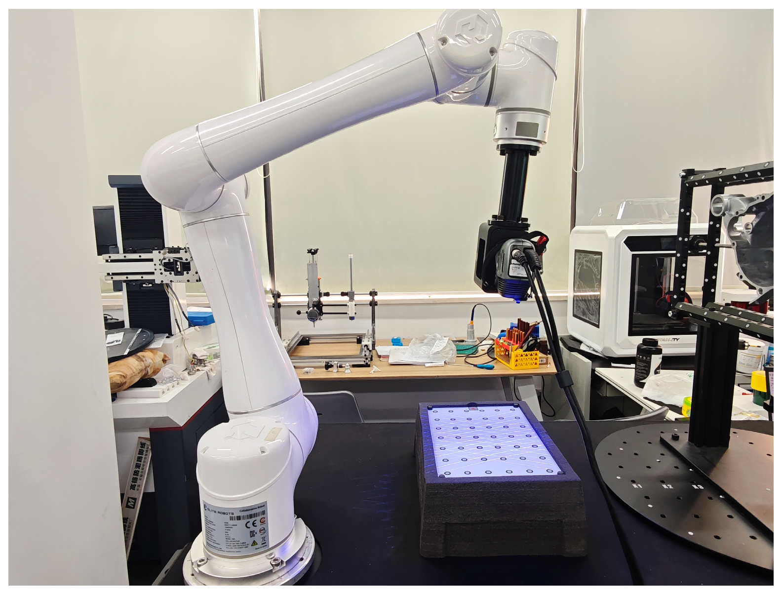
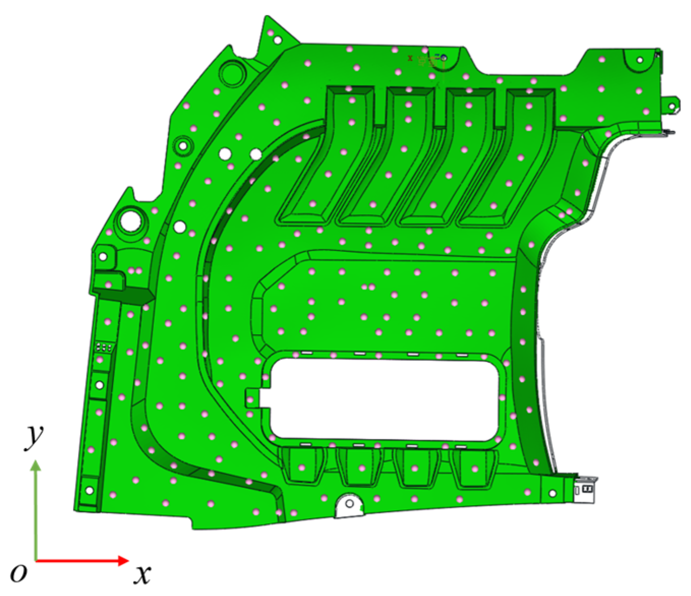
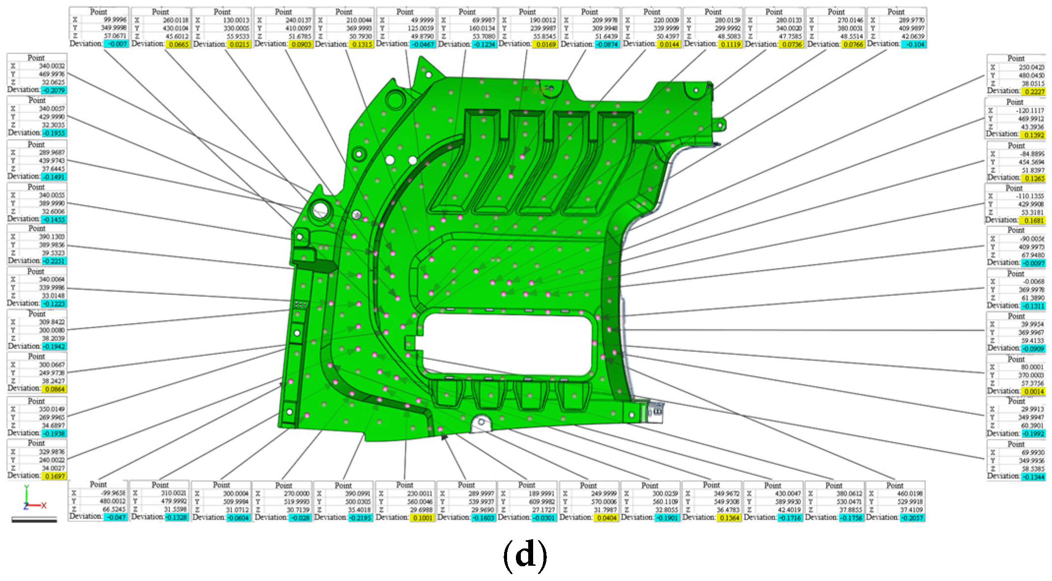
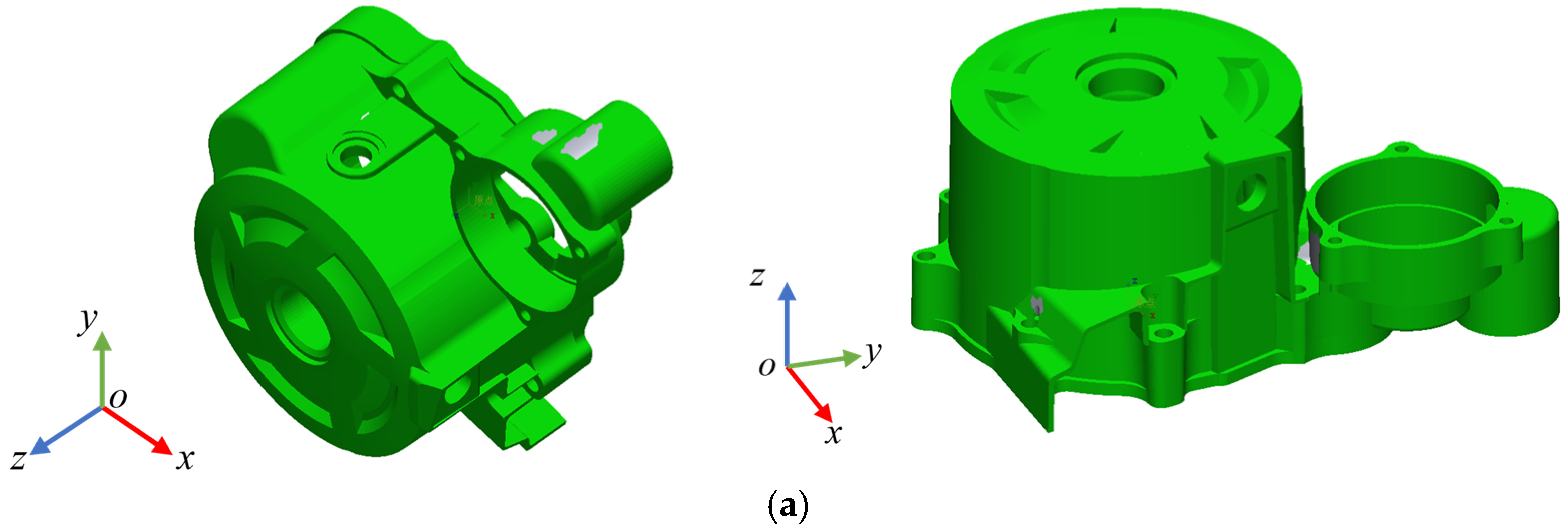
Although existing research on robot-assisted inspection has proven effective for handling specific features or part types, the critical issue of how to achieve comprehensive 3D inspection of complex parts in a single setup remains to be thoroughly investigated. To address the challenges, this paper proposes a Collaborative Robot-Based Automatic 3D Shape Inspection (CRAI) system aimed at achieving comprehensive, efficient, and high-precision 3D shape inspection of complex parts in a single setup. The system design is first developed, and the optimal measurement mode of the handheld scanner is analyzed. Subsequently, the method for generating adaptive viewpoints is discussed, followed by a focused investigation into the planning of spatial scanning paths for complex parts. The feasibility and effectiveness of the proposed inspection system were validated through experiments on two types of complex parts: one with an overall planar geometry and the other with an overall cylindrical geometry. The main contributions of this work are outlined as follows:
- (1)
A CRAI system is designed. This system performs 3D scanning tasks based on the optimal performance parameters of the scanner. By leveraging the multi-degree-of-freedom spatial motion capability of the collaborative robot, the system enables comprehensive, efficient, and high-precision 3D shape inspection of complex parts in a single setup.
- (2)
The spatial scanning path planning problem for complex parts is formulated as an SPP within the TSP framework, and an SAA is developed to solve this problem, thereby achieving optimal spatial scanning path planning for complex parts.
The rest of this work is structured as follows:
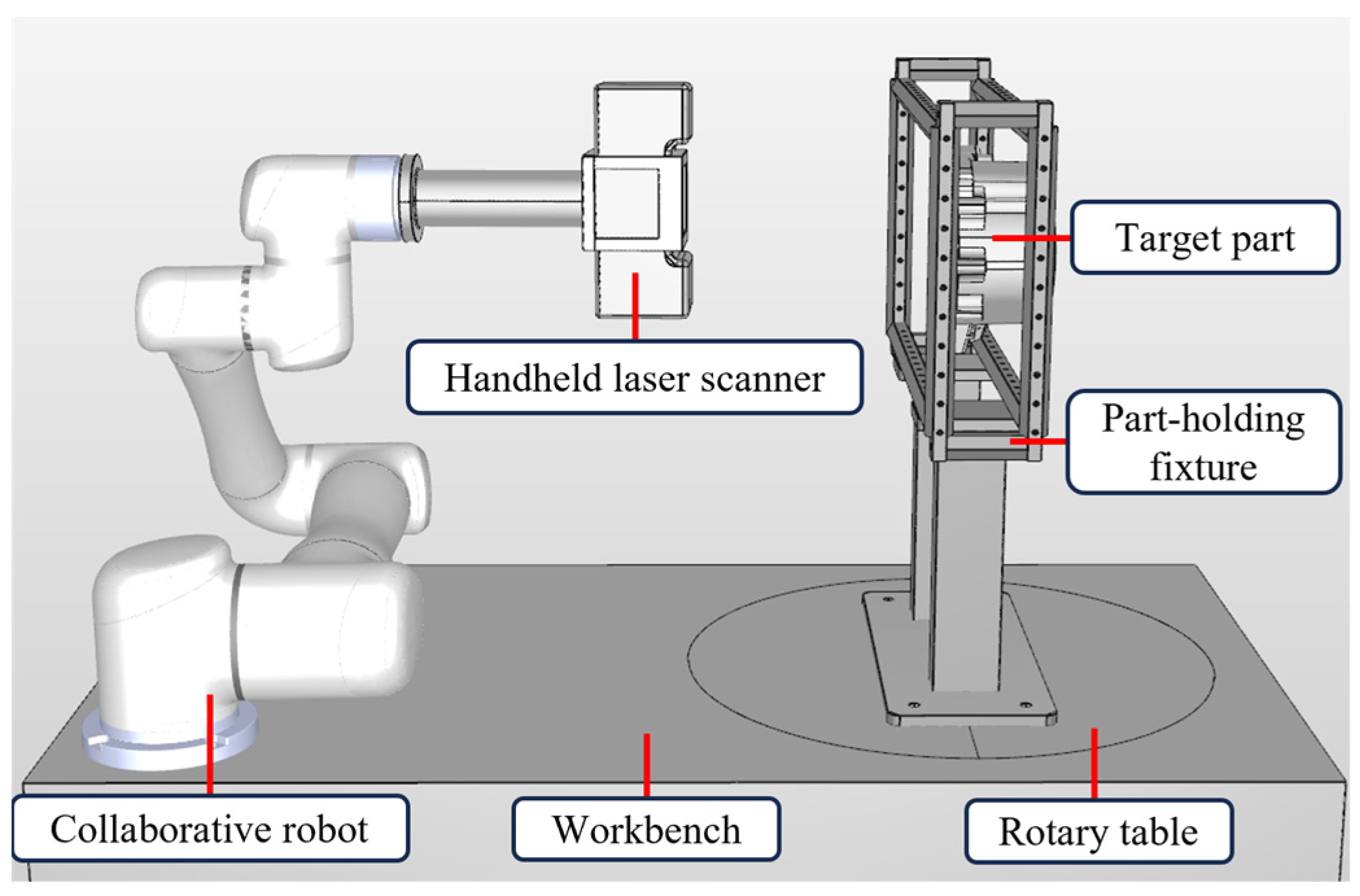
Section 2 describes the configuration of the collaborative robot-based 3D shape inspection system.
Section 3 elaborates on the inspection principle, including the generation of adaptive sampling points and scanning pose calculation, with an emphasis on scanning path planning.
Section 4 discusses experimental results. Finally, the conclusion of this work is presented in
Section 5.
3. Inspection Principle
3.1. Adaptive Viewpoint Sampling
The scanning viewpoint is defined as the spatial position of the origin of the sensor coordinate system during the laser scanning process. An ordered sequence of multiple scanning viewpoints forms the complete scanning path of the laser scanner. This paper investigates the generation and path planning of scanning viewpoints under the condition of known CAD models. The implementation utilizes Visual Studio 2019 software with MFC and Open Cascade (OCC) for complex part model import and visualization. The OCC framework enables surface segmentation, parameter extraction, and interactive operations including isoparametric curve generation, scanning viewpoint computation, and viewpoint visualization.
Adaptively distributed viewpoints can accurately capture the surface shape with a minimum number of points, thereby improving scanning efficiency. Adaptive viewpoint sampling begins with surface segmentation, dividing the complex part into planar and curved surface patches. The direction of isoparametric curves is then determined based on the curvature characteristics of these curved patches. Following this, a parameterization method is applied to discretize the surfaces into a series of points in a “surface-curve-point set” sequence. Based on these points, adaptive sampling of scanning viewpoints is performed, constrained by factors such as the effective length of the scanner’s laser line, the optimal working angle, and the optimal working distance. The specific method is described in the following subsection.
Both planar and curved surfaces can be represented through parametric methods:
In such representations, the coordinates
x,
y,
z of any point on the surface are scalar functions of parameters
u and
v. Isoparametric curves are defined as trajectories formed by varying one parameter while holding the other constant on the parametric surface. For instance, fixing
v =
v0 (where
v0 is constant) yields the isoparametric curve
L(
u):
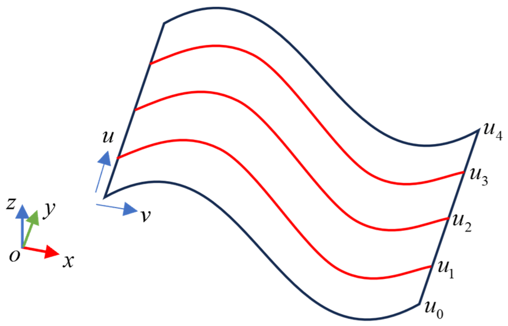
The selected isoparametric curves must adequately capture the geometric signatures of the surface to ensure measurement accuracy. Consider the surface in
Figure 4 with the parametric equation:
Geometric analysis reveals that the v-directional isoparametric curves more effectively characterize the cross-sectional profiles of this surface. Consequently, the surface should be discretized into clusters of isoparametric curves along the v direction. In this step, the spacing between u-direction isoparametric lines are determined by the laser’s effective scanning length, with an overlap of approximately 20% maintained between adjacent scanning tracks to ensure point cloud continuity and integrity.
When sampling measurement points on isoparametric curves, points should be concentrated in regions with significant curvature variation to fully capture geometric features. Adaptive sampling methods for free-form curves include equal arc-length sampling, equal chordal deviation sampling, and equal chord-height sampling. Research [
29] has demonstrated that equal chord-height sampling achieves superior characterization of high-curvature regions under fixed sample size constraints. Consequently, this method is adopted for curve sampling.
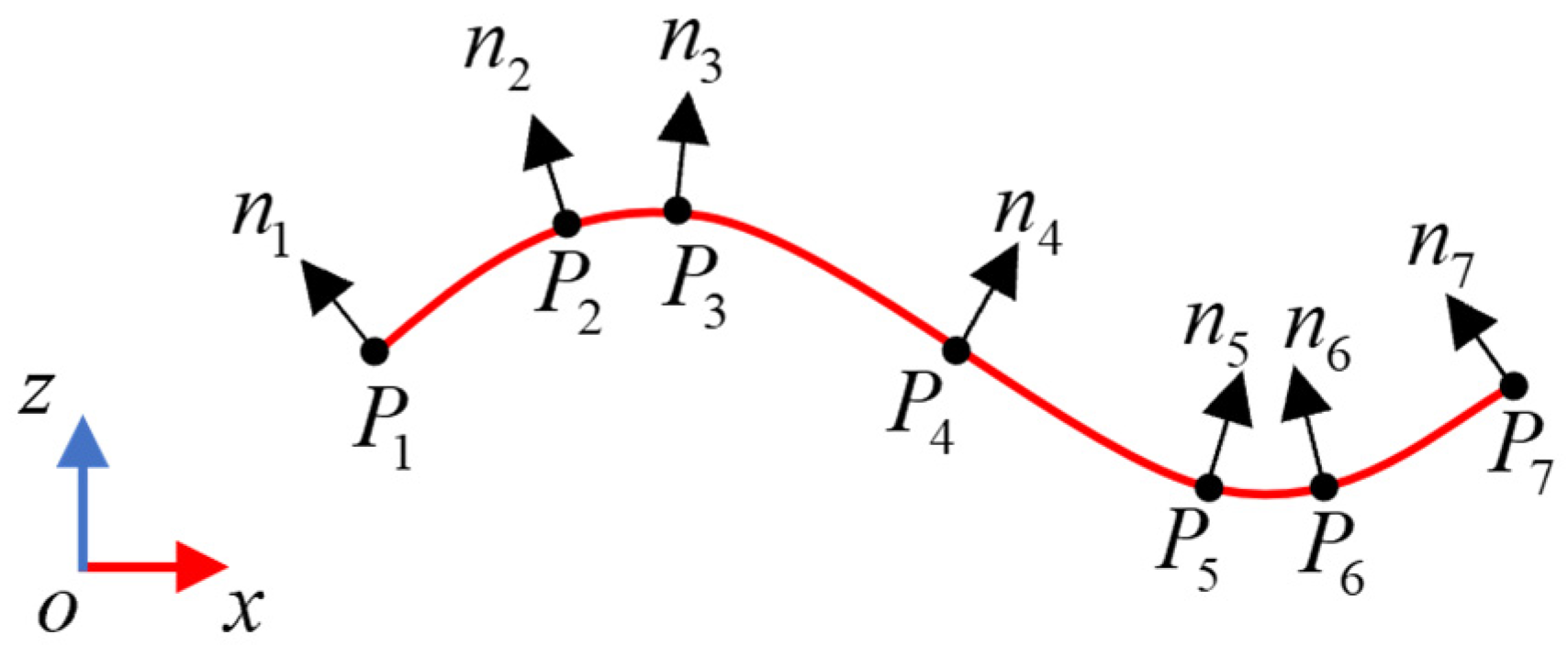
Figure 5 illustrates the result of equal chord-height adaptive sampling applied to an isoparametric line from
Figure 4, with the number of sampling points set to 7. As observed, regions of higher curvature exhibit a denser distribution of sampling points, whereas sparser sampling occurs in areas of lower curvature. The parametric values, coordinates and outward normal vectors
ni of the sampled points
Pi are stored for subsequent measurement path planning.
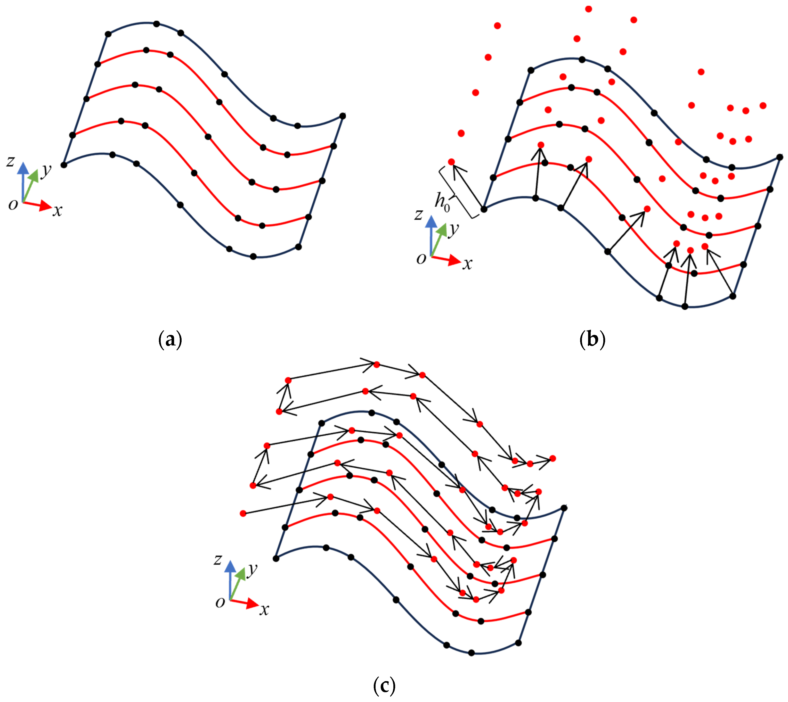
As shown in
Figure 6a, equal chord-height adaptive sampling is applied to all isoparametric curves of the surface in
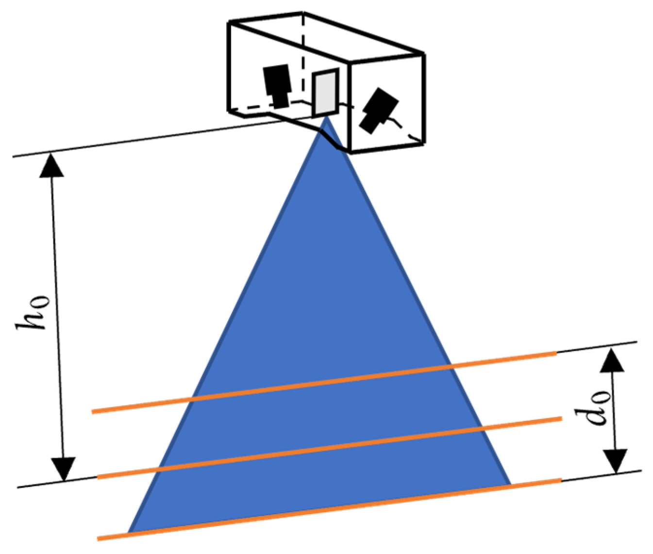
Figure 4. The complete scanning viewpoint set is generated by displacing all the sampled points along their outward normal vectors by the scanner’s reference distance
h0, as illustrated in
Figure 6b. The scanning path is then constructed by sequentially connecting scanning viewpoints on the same isoparametric curve with straight lines first, then linking the terminal scanning viewpoints of adjacent curves. The final scanning path is illustrated in
Figure 6c.
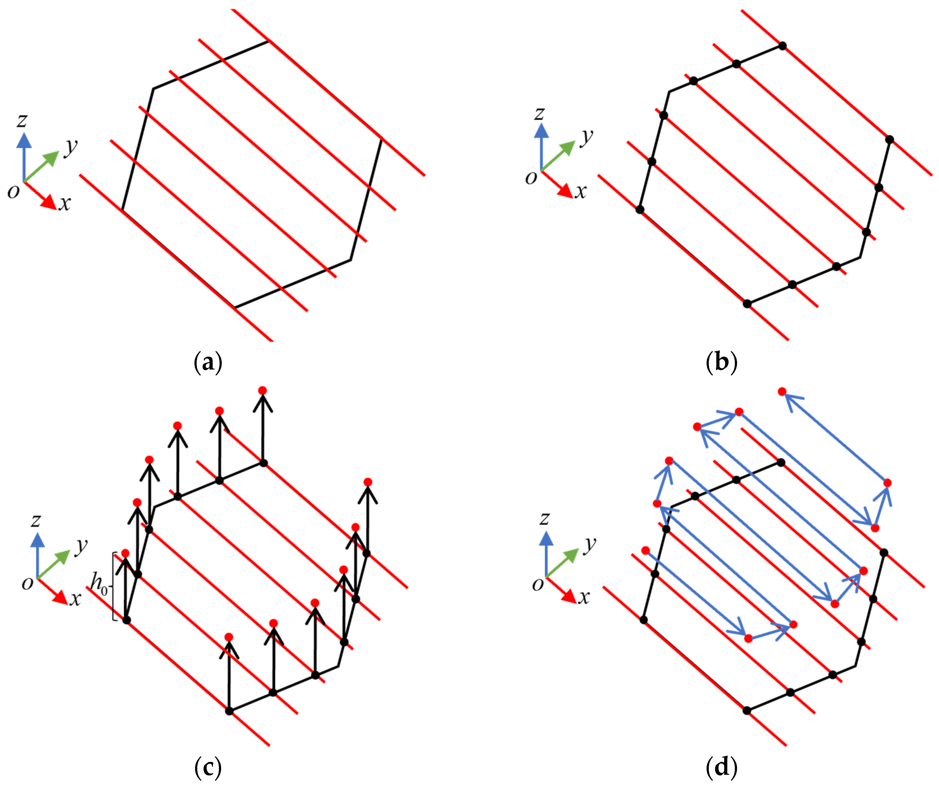
Since planar surfaces exhibit zero curvature, scanning viewpoint planning prioritizes coverage completeness. Consider the regular hexagonal plane in
Figure 7, which is defined parametrically as:
The scanning viewpoint acquisition process comprises the following steps:
- (1)
Parametrize the plane followed by isoparametric curve generation based on the scanner’s effective scanning width, as shown in
Figure 7a.
- (2)
Boundary intersection calculation for each isoparametric curve, illustrated in
Figure 7b.
- (3)
Displacement of all intersection points along the outward normal by the reference distance
h0 to yield scanning viewpoints, depicted in
Figure 7c.
- (4)
The sequential linear connection of viewpoints to form the scanning path is presented in
Figure 7d.
3.2. Scanner Pose Calculation
Based on the planned scanning viewpoint, the spatial coordinates, outward normal vectors, and scanning paths are determined. However, optimal scanning requires satisfying specific pose constraints during operation.
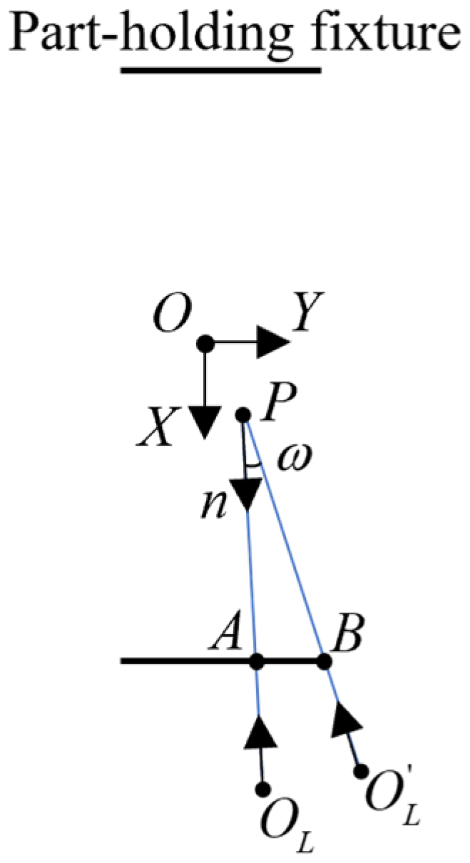
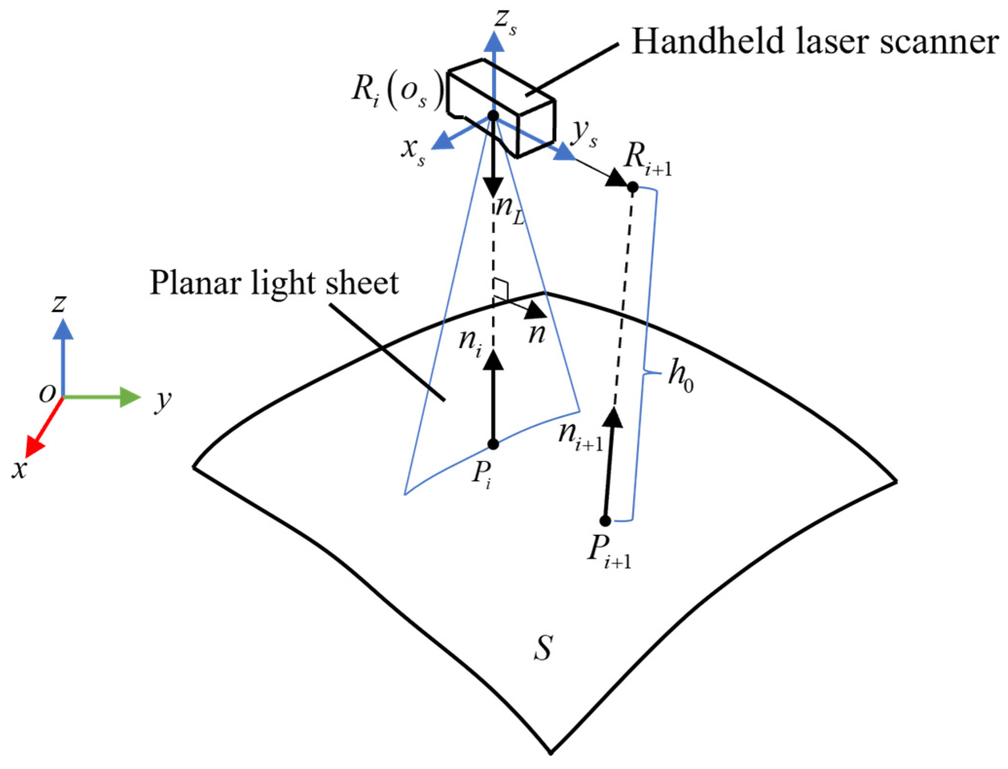
As shown in
Figure 8, in the measurement coordinate system
o-
xyz, let
Pi and
Pi+1 be adjacent sampling points on an isoparametric curve,
Ri and
Ri+1 denote corresponding scanning viewpoints,
represents the path vector,
ni is the outward normal at
Pi,
n is the laser plane normal vector, and
h0 is the reference distance between
Pi and
Ri.
The sensor coordinate system
os-
xsyszs of the handheld laser scanner is established with the emission point of the laser as the origin. In
Figure 8,
nL is the main axis direction vector of the laser, which is opposite to
zs and located in the laser plane. During the process of transporting the scanner from
Ri to
Ri+1, the following posture and position requirements must be met: the origin
os of the scanner sensor coordinate system should coincide with
Ri to ensure that the scanner is at the optimal measurement distance; the main axis direction vector
nL of the laser should coincide with the outward normal vector
ni of the sampling point
Pi to ensure that the scanner is at the optimal measurement angle; and the laser plane on the scanner should be perpendicular to the path vector
. After meeting the above posture requirements, the scanner should maintain its current posture and move along a straight trajectory to the next scanning viewpoint
Ri+1.
To achieve the predefined spatial position and orientation, the scanner’s current pose in the measurement coordinate system
o-xyz must first be determined. Prior to the pose calculation, laser plane calibration [
30] is required to obtain the plane equation and its unit normal vector
n. Let the rotation matrix be
R,
,
,
,
, yielding the following equations:
Two local coordinate systems are established:
From Equation (5), it follows that:
Combining Equations (5) and (7):
After R is obtained, the scanner orientation in o-xyz can be determined through the rotation matrix R.
3.3. Scanning Path Planning
3.3.1. Problem Analysis
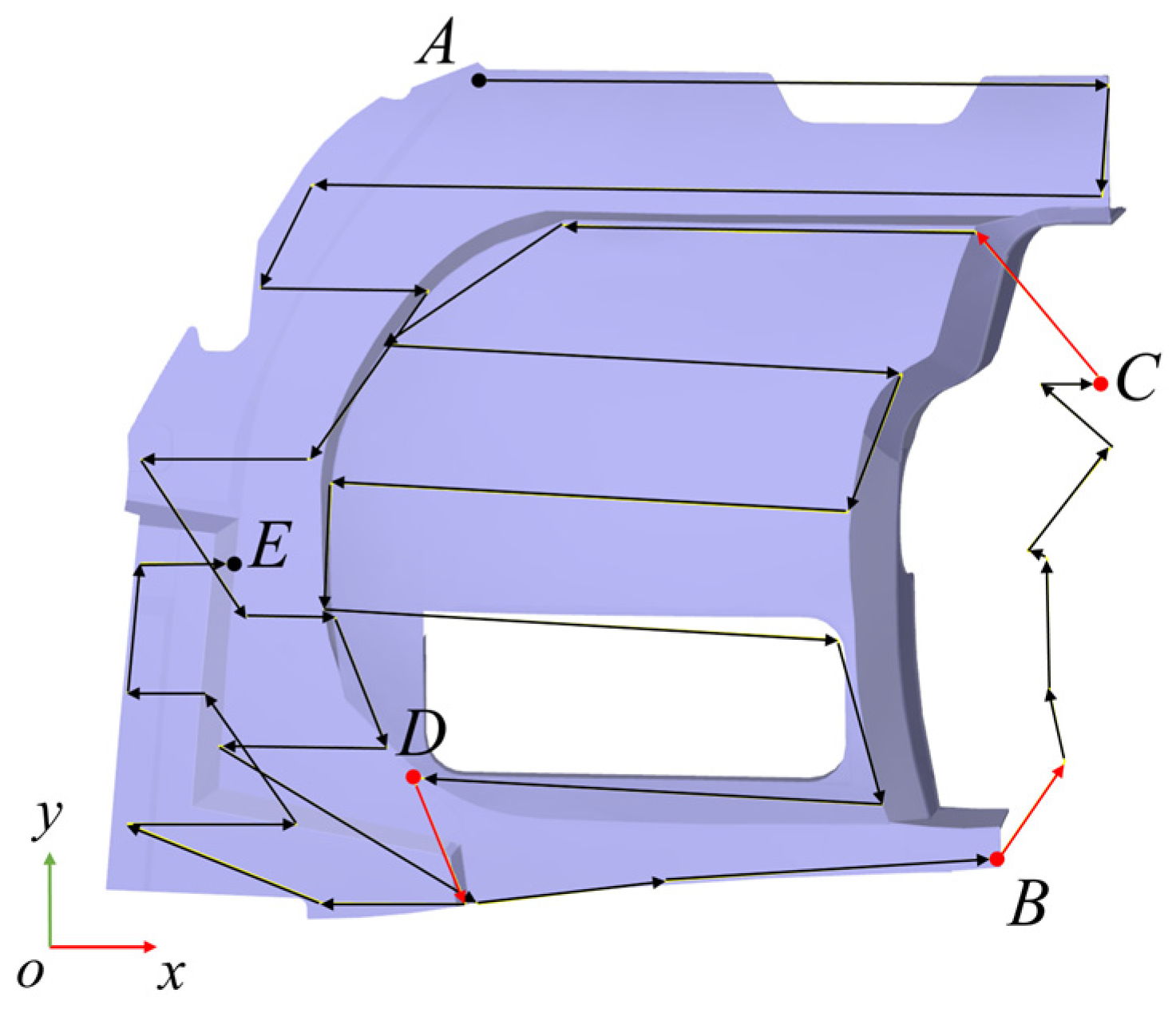
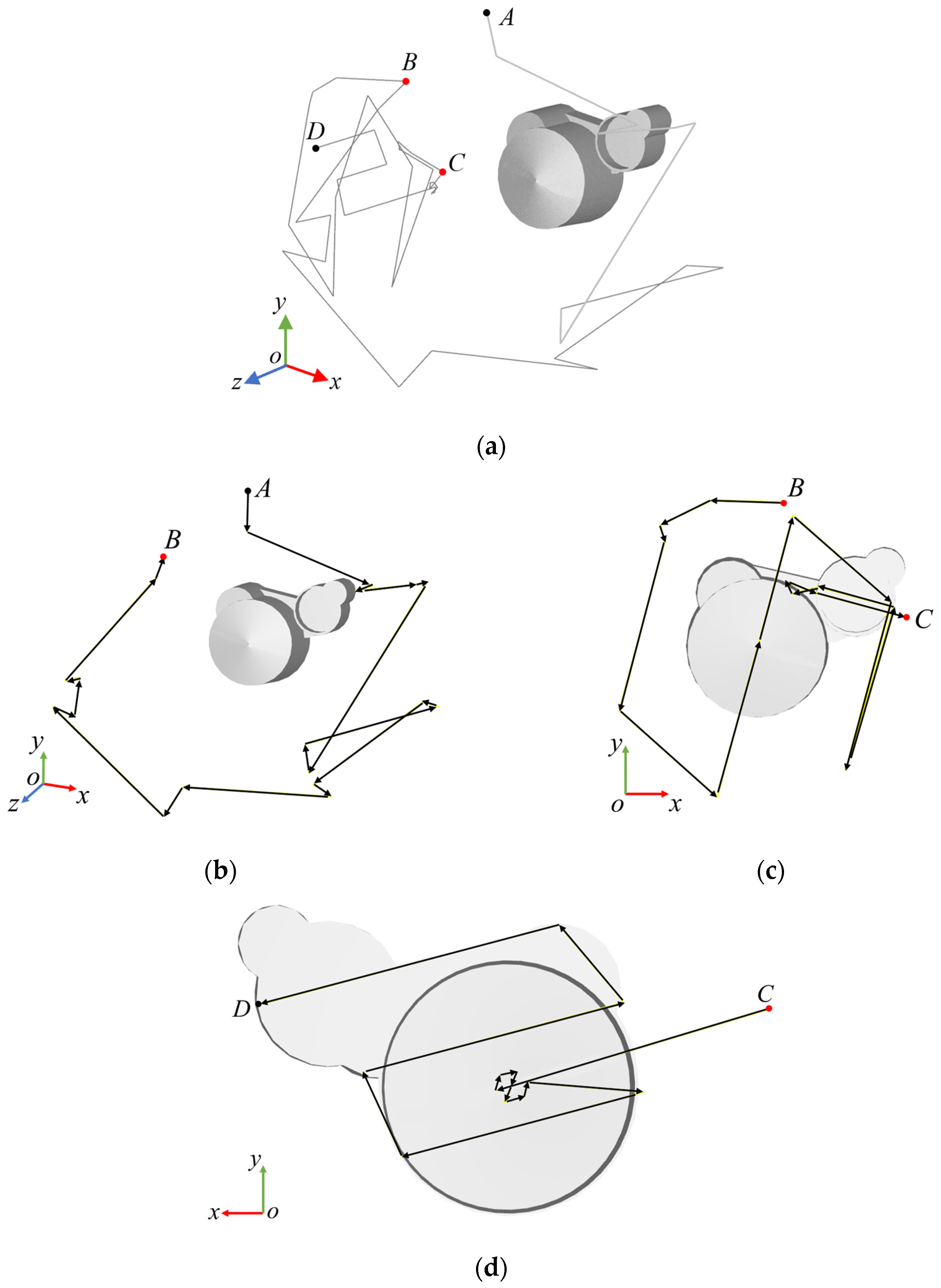
During actual measurement, the surface of complex parts needs to be divided into multiple measurement regions. When scanning accessibility becomes challenging, the relative position between the measurement region and the collaborative robot can be adjusted via the rotary table, allowing the scanner to achieve optimal measurement mode. Region segmentation employs curvature-based analysis, where surfaces with curvature variations below a specified threshold are grouped into the same region [
31]. This study decomposes path planning into two subproblems: Intra-region planning within individual measurement regions, and Inter-region transition planning between distinct regions.
For intra-region planning, scanning paths are generated by connecting the viewpoints along the same isoparametric curve, and linking the terminal viewpoints of adjacent curves, as detailed in
Section 3. The subsequent discussion focuses on inter-region path planning.
To achieve complete and efficient scanning of complex parts, the planning of scanning paths is essential. This problem can be regarded as a 3D extension of the TSP [
32]. In the classical TSP, a salesman departs from his home city, visits all specified cities exactly once, and returns to the origin, aiming to find the shortest possible route. In this paper, we adapt this model by treating each “city” as a “scanning viewpoint” and defining the “tour length” as the total “travel distance of the laser scanner”.
The current mainstream TSP solving methods include Simulated Annealing (SA) [
33], Tabu Search (TS) [
34], Neural Networks (NN) [
35], Ant Colony Optimization (ACO) [
36], Genetic Algorithms (GA) [
37], Hybrid Optimization [
38], etc. Classical methods, primarily employed for solving large-scale TSP, are often limited by insufficient robustness or excessive computational time. The scanning path planning problem investigated in this paper involves a relatively small number of measurement regions, classifying it as a small-scale TSP with the number of nodes
n ≤ 20. Meanwhile, it differs from the classic TSP in that it does not require the scanner to return to the starting point, meaning no closed loop is necessary. Additionally, the selection of the next path node is divided into mandatory and optional choices. In light of these characteristics, the path planning problem is transformed into an SPP within a network under the TSP framework. Then, by leveraging the “local optimality leading to global optimality” strategy derived from the Dijkstra greedy algorithm [
39]. An SAA is then constructed for solving the path planning problem.
3.3.2. Path Network Construction for SPP
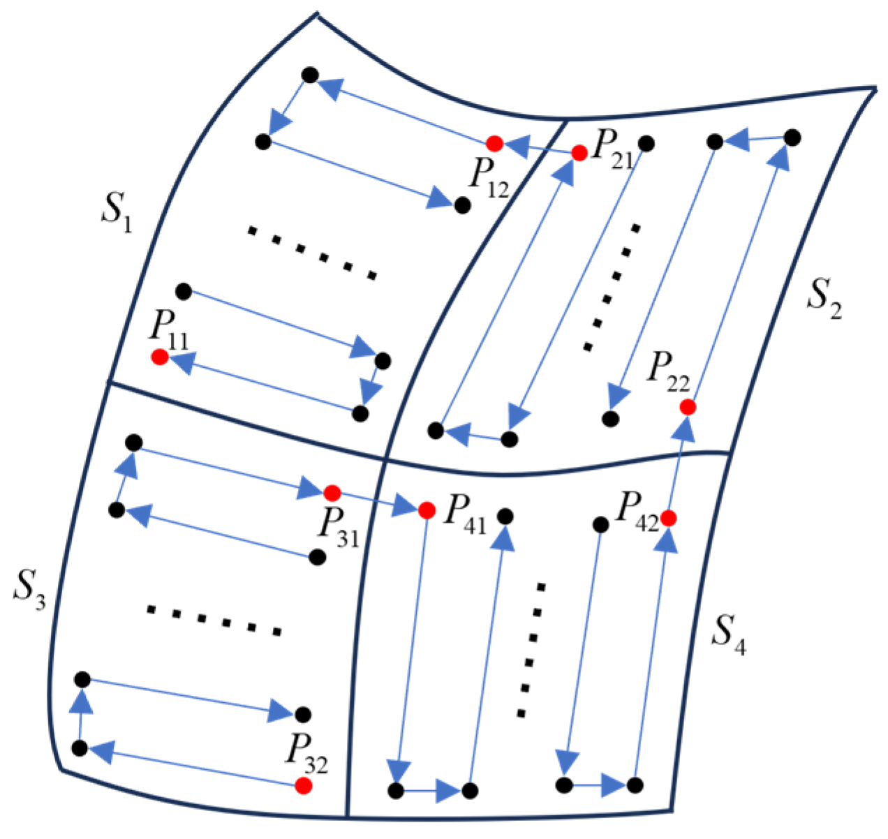
As shown in
Figure 9, assume there are four measurement areas
Si (
i = 1, 2, 3, 4). Within each area, there are two viewpoints
Pi1 and
Pi2 (which are not offset for clarity).
Pi1 and
Pi2 serve as the commencement and termination points for each other regarding the intra-area scan path. To clarify, when
Pi1 is the starting point,
Pi2 is the end point, and vice versa. Since the scanning path within each area has been pre-planned, the selection of the next viewpoint within an area is deterministic. However, the next viewpoints for inter-area travel can be arbitrarily selected.
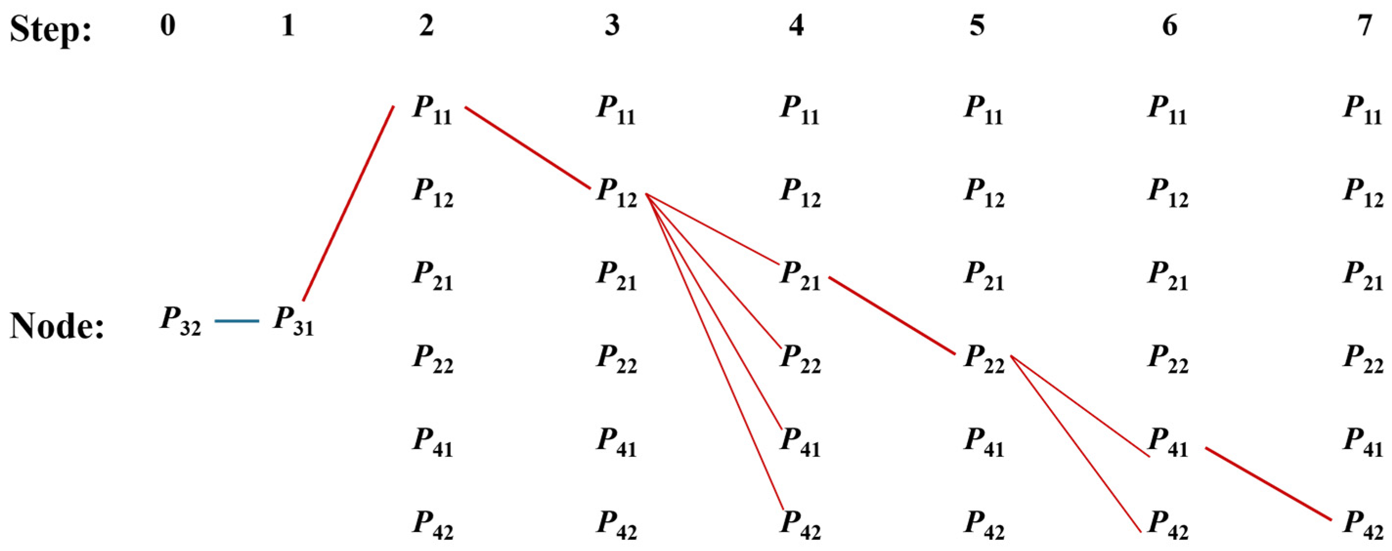
Subsequently, a path network graph is constructed based on the principle: “select a candidate node deterministically if it resides within the same region; otherwise, choose arbitrarily from candidate nodes outside the current region.” As illustrated in
Figure 10, assuming the measurement path initiates from point
P32 (i.e., the node for Step 0 is defined as
P32), the node for Step 1 is
P31. This is because both
P32 and
P31 belong to the same region
S3, thereby completing the scan of
S3.
In Step 2, from P31, there are six candidate nodes located outside its current region: P11, P21, P22, P41, and P42. Assuming P11 is selected, then the node for Step 3 is P12, thereby completing the scan of area S3. Subsequently, in Step 4, from P12, there are four candidate nodes outside its region: P21, P22, P41, and P42. If P21 is selected, the node for Step 5 is determined as P22, which finalizes the scan of area S2. In Step 6, from P22, there exist two candidate nodes external to its region: P41 and P42. Supposing P41 is selected, the node for Step 7 is consequently P42, thereby finalizing the scan of area S2 and, consequently, completing the scanning of all measurement areas.
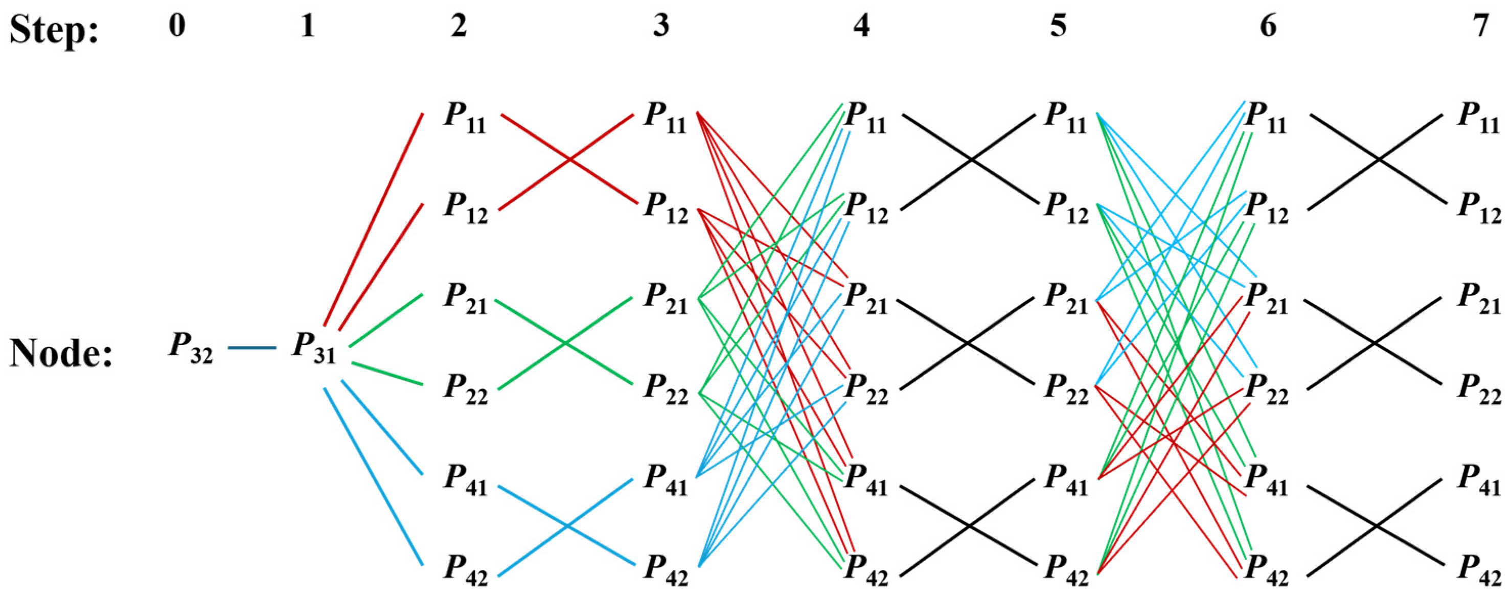
By traversing all candidate points from the aforementioned steps, a path network graph can be constructed to solve the SPP of the laser scanner, as illustrated in
Figure 11. The shortest path planning is subsequently performed based on this network graph.
3.3.3. Shortest Scanning Path Planning
First, based on the network diagram shown in
Figure 11, an 8 × 8 distance matrix
is constructed:
Subsequently, values are assigned to the distance matrix. For any two points with identical indices, their distance should be 0 (e.g.,
P11P11 = 0). For two viewpoints within the same region, as their selection is deterministic, their distance is also set to 0. The distances for all other pairs are configured based on the proximity relationships depicted in
Figure 9. The assigned distance matrix is presented as follows:
where
d represents the proportionality coefficient.
Subsequently, the SAA is executed for shortest path planning. Let denote the shortest path length when node Pij is selected at the k-th step. Let represent the predecessor node of Pij, chosen at the k-th step with the objective of minimizing the path length. Let or PijPmn signify the distance between Pij and Pmn.
In Step 0, assuming
P32 is designated as the starting point, the following initial conditions are established:
In Step 1, as illustrated in
Figure 11, since the predecessor node of
P31 is
P32,
can be expressed as:
From Equations (10) and (11), it follows that
P31P32 = 0. Consequently:
In Step 2, as can be seen from
Figure 11, the predecessor of
P11 is
P31. Therefore,
can be expressed as:
From Equations (10) and (11), it follows that
P11P31 = 4
d. Given that
from Equation (15), the following results are obtained:
Similarly, by applying the same calculation to the other nodes in Step 2, the shortest path lengths and the corresponding predecessor selections for all nodes can be obtained, as listed in
Table 1.
In Step 3, as illustrated in
Figure 11, the predecessor of
P11 is
P12. Consequently, the path length is calculated as:
From Equations (10) and (11), it follows that:
Similarly, applying the same calculation to the other nodes in Step 3 yields the results presented in
Table 2.
In Step 4, as shown in
Figure 11, the candidate predecessor nodes for
P11 are
P21,
P22,
P41, and
P42. Therefore, the shortest path length is determined by evaluating the minimum over the following expressions:
From Equations (10) and (11), it can be obtained that:
Since selecting
P42 as the predecessor node yields the minimum path length, we have:
Similarly, applying the same calculation process to the other nodes in Step 4 yields the results presented in
Table 3.
In Step 5 and Step 6, following the computational procedure outlined in Step 3 and Step 4, respectively, the results shown in
Table 4 and
Table 5 were obtained.
In Step 7, as illustrated in
Figure 11, the predecessor of
P11 is
P12. Consequently, the path length is calculated as follows:
From Equations (10) and (11), we obtain:
Similarly, applying the same computational method to the remaining nodes in Step 7 yields the results presented in
Table 6.
From
Table 6, the shortest path length is determined to be
, with the terminal node being
P11, and the predecessor of
P11 is
P12. Tracing back through the tables: from
Table 5, the predecessor of
P12 is
P21; from
Table 4, the predecessor of
P21 is
P22; from
Table 3, the predecessor of
P22 is
P42; from
Table 2, the predecessor of
P42 is
P41; from
Table 1, the predecessor of
P41 is
P31; and from Equation (16), the predecessor of
P31 is
P32. Therefore, the shortest scanning path for the four measurement areas
Si (
i = 1, 2, 3, 4), as conceptually shown in
Figure 9, is reconstructed as:
3.4. Trajectory Generation for Collaborative Robots
The scanning path represents the motion trajectory of the scanner’s sensor coordinate frame origin (Os). Since spatial motion and orientation adjustments are executed by the collaborative robot, the scanning path must be converted into the motion trajectory of the collaborative robot, which entails converting the path into the robot’s motion parameters.
The Denavit-Hartenberg (DH) method serves as the fundamental methodology for robot kinematic modeling [
40]. By standardizing joint coordinate system establishment rules, it enables accurate geometric and kinematic descriptions. This approach establishes the theoretical foundation for robot motion control and trajectory planning, with two principal variants: Standard DH (SDH) and Modified DH (MDH) [
41].
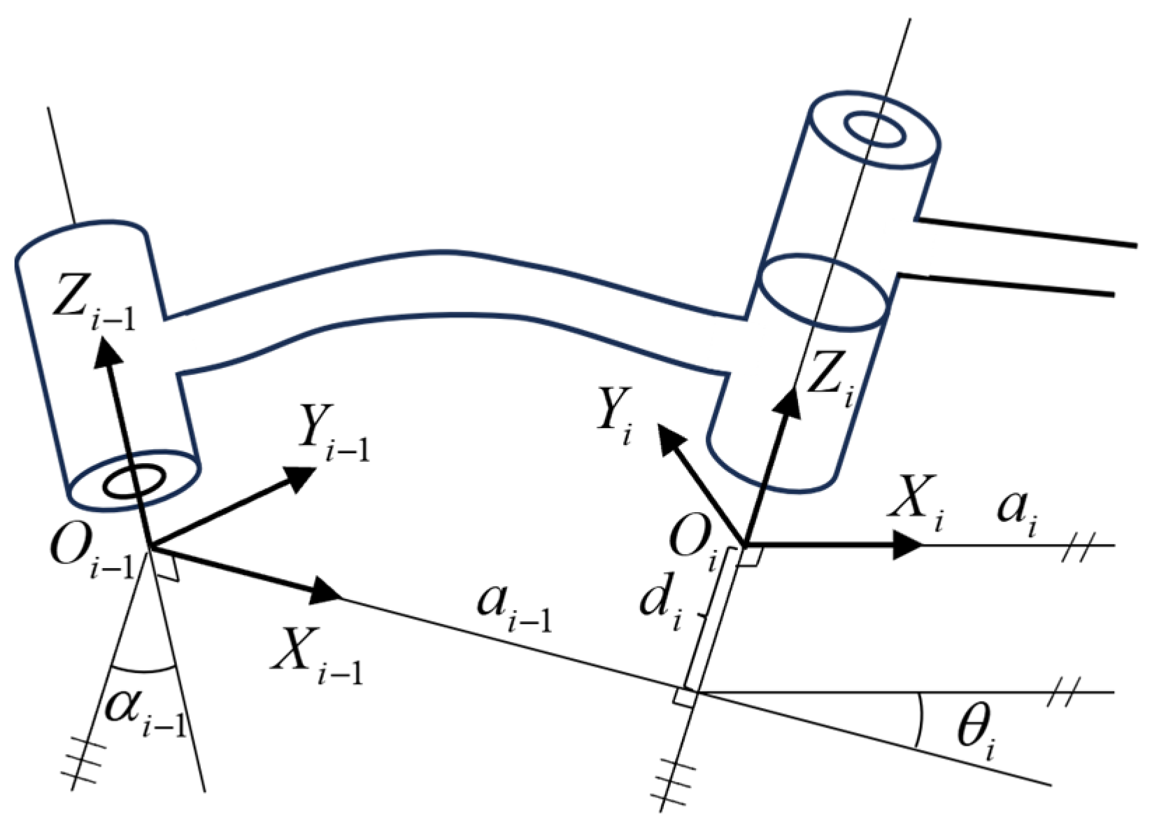
As shown in
Figure 12, the MDH model defines four parameters with the following geometric interpretations:
: Rotation angle about the xi axis from zi to zi+1,
: Translation distance along the xi axis from zi to zi+1,
: Rotation angle about the zi axis from xi−1 to xi,
: Translation distance along the zi axis from xi−1 to xi.
The MDH transformation matrix between consecutive frames is given by:
This study establishes the MDH model for the collaborative robot with the following parameter specifications in
Table 7.
Substituting the DH parameters into the MDH formula yields the homogeneous transformation matrix
:
where
denotes the homogeneous transformation matrix from the robot base frame to the end-effector frame, encoding both rotation and translation, and
represents the transformation matrix between adjacent joint frames
i − 1 and
i.
Inverse kinematics represents the inverse process of forward kinematics, establishing a mapping from Cartesian space to joint space based on a known end-effector pose matrix, and solving for joint variable values. This procedure is more important than forward kinematics in trajectory planning and motion control. Commonly used solution methods include geometric approaches, numerical iteration, and algebraic methods. Among these, algebraic methods are capable of computing all closed-form solutions with high accuracy. In robotic inverse kinematics solving, to ensure the uniqueness and smoothness of trajectory execution, this paper selects the optimal solution based on the minimal-displacement criterion in joint space. The calculation formula is defined as follows:
where
denotes the calculated angular deviation,
represents the group
k inverse solution set, and
corresponds to the initial joint angles.
5. Conclusions
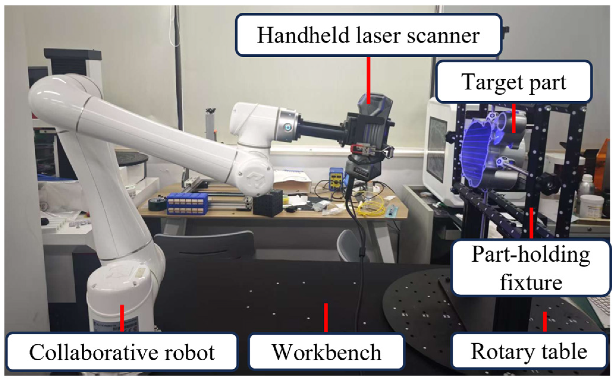
This research proposed a collaborative robot-based approach for the automated 3D shape inspection of complex parts. An inspection system was developed by integrating a handheld laser scanner onto the end-effector of a collaborative robot, combining with a rotary fixture. This configuration endows the handheld laser scanner with automated, multi-degree-of-freedom spatial scanning capabilities. The problem of spatial scanning path planning for complex parts was formulated as an SPP within the TSP framework. An SAA was developed to solve this problem, which effectively determines the optimal scanning path. The developed inspection system is capable of performing 3D scanning of complex parts along the planned path while adhering to the optimal measurement parameters of the handheld scanner. This allows for comprehensive, efficient, and high-precision 3D shape inspection of complex parts in a single setup. Simulations and experiments were conducted to validate the proposed collaborative robot-based inspection method. The results demonstrate that, compared to prior methods, the proposed approach achieves higher efficiency and accuracy in the 3D shape inspection of complex parts. Moreover, these advantages become increasingly pronounced as the geometric complexity of the measured part increases.
Although the proposed method has proven effective, several limitations remain that warrant further investigation. In the current study, the scanning plane of the handheld laser scanner was simplified to a single primary plane for path planning purposes. However, actual scanners may employ multiple or even dozens of laser planes operating simultaneously. Future work will address measurement path planning considering multiple scanning planes. Furthermore, in the present method, to facilitate the determination of the scanner’s working distance, the surfaces of complex parts were simplified, and fine features were filtered. Subsequent research will focus on restoring realistic working conditions by developing an algorithm to determine the scanning distance on complex surfaces. Additionally, dynamic comparison between scan data and the model, secondary measurement of unscanned regions, and dynamic data simplification are also important considerations for future investigation.