Research on Control Strategy of Electromagnetic Pneumatic System Based on Fuzzy PID and Exploration of Flow Estimation Method for IWT

Abstract

Accurate real-time pneumatic flow estimation offers a cost-effective alternative to expensive, bulky flow meters, yet persistent challenges stem from complex valve environments, high nonlinearity, and stringent precision requirements. This paper introduces a novel control framework integrating fuzzy PID dynamic tuning with adaptive wavelet threshold denoising, synergistically optimizing fuzzy PID and improved wavelet transform (IWT) to simultaneously enhance control accuracy and signal quality. Experimental validation demonstrates a 35% reduction in spool displacement overshoot versus conventional PID control. IWT integration improves flow estimation signal-to-noise ratio (SNR) by 65% relative to hard/soft thresholding methods while reducing root mean square error (RMSE) by 49%. The approach significantly outperforms mainstream techniques in dynamic response and noise immunity, enabling precise proportional valve flow measurement. This algorithm-driven strategy replaces high-cost sensors, reducing industrial maintenance requirements. Especially applicable to electromagnetic pneumatic systems in harsh environments, it establishes a reliable framework for proportional valve flow control.

1. Introduction

Electromagnetic pneumatic systems have gained significant traction in industrial applications due to their superior speed compared to traditional pneumatic systems. Proportional control valves, as integral components of pneumatic systems, are employed to regulate the opening of the valve spool, thereby achieving the desired flow rate and pressure within the system. The overall performance of the system is contingent upon the functionality of the proportional control valve. In actual operating conditions, external sensors are often used in conjunction with proportional control valves to provide feedback to the actuators. However, due to the harsh operating environments in which they are employed, external sensors are prone to damage, which may result in economic losses and safety incidents. Consequently, there is a pressing need for research on the utilization of proportional control valves for direct flow regulation [1]. At present, electromagnetic pneumatic valves employed for the regulation of airflow are predominantly classified into two categories: servo valves and quick-switching valves [2]. Servo valves offer high precision and linearity but are expensive and structurally complex. Quick-switching valves are simple and inexpensive but have weaker linearity [3].

Proportional control valves utilize the flow rate required for system operation as the control target, leveraging the measured flow rate as feedback to establish a closed-loop feedback control mechanism. Consequently, there is an imperative for research to be conducted on control strategies for electromagnetic pneumatic systems and the exploration of flow estimation methods. A considerable body of research has examined the modeling and control of electromagnetic pneumatic systems, with a predominant focus on cylinders and pneumatic valves [4,5,6,7,8,9]. Electromagnetic pneumatic systems utilize a range of control methodologies. In their research, Hadgson et al. developed an electromagnetic pneumatic system for robots, utilizing a sliding mode controller (SMC) to control cylinder position [10]. Similarly, Leephakpreeda et al. developed a fuzzy logic controller (FLC) for pneumatic artificial muscles [11] and evaluated the performance of the FLC for controlling high-precision pneumatic systems in simulations and experimental prototypes [12]. In [13], Swider et al. A proposed control scheme utilizes a PIC microcontroller. Taghizadeh et al. [14] investigated the influence of pneumatic loops on input-output behavior and enhanced control performance using a controller based on a linear strategy rather than a nonlinear scheme.

Furthermore, scholars have conducted extensive research on flow estimation measurement methods. Xie et al. [15] noted that the flow emission coefficient demonstrates substantial nonlinearity under conditions of valve opening and pressure difference. To account for this nonlinearity, the emission coefficient was determined through computational fluid dynamics (CFD) simulation. Valdés et al. [16] derived flow coefficients by introducing functions based on the Reynolds number. Reference [17] proposed an experimental procedure to evaluate the emission coefficient as a function of valve opening area, pressure difference, and temperature. Zhang et al. [18] implemented an AdaBoost neural network to infer flow measurements, establishing correlations between flow velocity and various factors, including slide valve displacement, pressure difference, and temperature. In light of these findings, the researchers implemented AdaBoost technology to address the overfitting issue arising from the learning process within the BP neural network, thereby enhancing the model’s precision. Åman et al. [19] adopted a cubic polynomial equation, utilizing pressure difference as an independent variable for flow rate calculation, thereby attaining a balance between accuracy and computational efficiency. Ding et al. [20] refined the aforementioned method by incorporating particle swarm optimization to optimize the parameters of the BP neural network. Sitte et al. [21] employed the aforementioned three techniques to infer the flow measurement of the seat valve and conducted a comparison, ultimately concluding that the most accurate fitting results were obtained.

While the aforementioned methodologies have yielded satisfactory outcomes in the domains of pneumatic system control and flow estimation, significant challenges persist in their practical implementation. Existing pneumatic control system research generally struggles to balance control accuracy and computational efficiency under nonlinear dynamic characteristics and complex noise interference. The operational characteristics of pneumatic proportional electromagnetic valves frequently manifest nonlinear features, including flow-pressure characteristics and opening-flow characteristics. This nonlinearity poses significant challenges in the design and implementation of control algorithms, making it difficult to accurately describe and predict the behavior of electromagnetic valves. Additionally, electromagnetic interference and mechanical vibrations in industrial environments have been shown to cause sensor signal distortion, significantly reducing the accuracy of flow estimation measurements. Noise interference has been identified as a significant problem. For instance, flow sensors have been shown to produce erroneous readings due to noise, resulting in deviations in the control system’s adjustment of the pneumatic electromagnetic proportional valve’s opening. This, in turn, has been observed to affect the control accuracy of gas flow. Furthermore, the presence of noise has been demonstrated to exert an influence on the computational and decision-making processes of the controller. The presence of noise in input or feedback signals may cause the controller to make incorrect judgments, resulting in the issuance of incorrect control commands and further reducing control accuracy. On the other hand, existing control algorithms are mostly based on pre-set models and parameters, lacking self-learning capabilities, and heavily reliant on high-precision flow sensors, which come with issues such as high costs, susceptibility to damage, and difficult maintenance.

While advanced nonlinear control strategies have been successfully applied to pneumatic muscle actuators in rehabilitation applications [22,23], these methods typically focus on position tracking and human–robot interaction, where model uncertainties are addressed through disturbance observers or sliding mode control. In contrast, the present work targets industrial proportional valve flow control, where the primary challenges are flow nonlinearity, sensor noise, and embedded hardware constraints. The proposed fuzzy PID + IWT framework offers a lightweight solution suitable for real-time implementation on low-cost microcontrollers, which distinguishes it from computationally intensive approaches required in rehabilitation exoskeletons.

The proposed study presents a cooperative control framework that integrates a fuzzy PID and an enhanced wavelet threshold (IWT) mechanism. The fuzzy PID parameters ($K_{\mathrm{p}}$, $K_{\mathrm{i}}$, $K_{\mathrm{d}}$) are dynamically adjusted using fuzzy rules, thereby compensating for the nonlinear characteristics inherent in the electromagnetic pneumatic system, including the LuGre friction memory effect. The experimental findings indicate that the overshoot is diminished by 35% in comparison to the conventional PID. The proposed approach involves the implementation of an adaptive wavelet threshold denoising algorithm, a sophisticated mathematical model that integrates a decaying sine function with an exponential noise reduction mode. This innovative approach effectively suppresses high-frequency noise while preserving the nuances of the flow signal, thereby enhancing the signal-to-noise ratio (SNR) by 65% and reducing the root mean square error (RMSE) by 49%. The algorithm’s efficacy is further validated through its integration of electromagnetic, mechanical, and fluid dynamics models—a multifaceted fusion enabling multiphysics field coupling simulations. By eliminating reliance on high-cost external sensors, the method substantially mitigates maintenance risks in harsh operating environments. This system delivers a high precision, robust flow control solution for industrial proportional valves, thereby offering direct industrial application value.

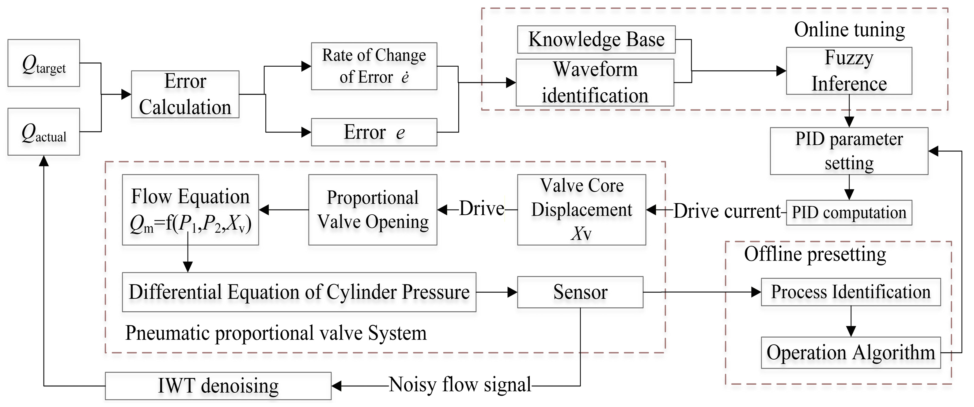
The overall control pipeline proceeds as follows: (a) Multi-physics modeling (Section 2), the proportional valve flow equation, LuGre friction model, cylinder pressure differential equation, and force equilibrium equation are coupled to form the plant model. (b) Fuzzy PID controller design (Section 3), the error e and error change rate ė between the target and actual flow are used as inputs; fuzzy inference dynamically adjusts $K_{\mathrm{p}}$, $K_{\mathrm{i}}$, $K_{\mathrm{d}}$ online to compensate for plant nonlinearity. (c) Improved wavelet threshold (IWT) denoising (Section 4), noisy sensor signals are processed via adaptive wavelet thresholding before being fed back to the controller, improving signal-to-noise ratio. (d) Experimental validation (Section 5), fuzzy PID control performance, denoising effectiveness, and multi-method flow estimation comparisons are presented.

2. Proportional Control Valve Multi-Physics Field Coupling Modeling

Due to the inherent nonlinear characteristics of pneumatic systems, such as the high compressibility of gases and the real-time variations in the parameters and variables of the gas within the cylinder during its movement, the accurate modeling of pneumatic systems poses significant challenges. The establishment of a system model involves the formulation of reasonable assumptions regarding the control system, with the objective of simplifying the mathematical representation of the system. The following is a list of the relevant points:

• The working medium in the pneumatic system—air—is treated as an ideal gas;
• Air leakage between the cylinder and the external environment, as well as between the two chambers of the cylinder, is neglected;
• The air flow in the pneumatic system is assumed to be an isentropic adiabatic process;
• The air supply pressure and atmospheric pressure are constant;
• The temperature and pressure of the gas are equal at all points within the same chamber.

2.1. Proportional Valve Core Module Modeling

The core module of the proportional valve principally comprises the flow equation and nonlinear characteristics of the proportional valve, as well as compensation for the friction model.

2.1.1. Flow Equation and Nonlinear Characteristics of Proportional Valves

In the context of practical servo control systems, the flow process of gases is characterized by a high degree of complexity. In the context of pneumatic component research, the flow process of an ideal gas with constant entropy through a nozzle is employed as a model. When calculating the flow rate at the valve opening, the Sanville flow formula is generally employed:

$$q_{\mathrm{m}} = A{P}_{\mathrm{s}}\sqrt{{\displaystyle \frac{k}{\mathrm{R}T}}{\displaystyle \frac{2}{k -1}}}\sqrt{{\left({\displaystyle \frac{P_{\mathrm{d}}}{P_{\mathrm{s}}}}\right)}^{{\displaystyle \frac{2}{k}}} - {\left({\displaystyle \frac{P_{\mathrm{d}}}{P_{\mathrm{s}}}}\right)}^{{\displaystyle \frac{k+1}{k}}}}, 0.528 < {\displaystyle \frac{P_{\mathrm{d}}}{P_{\mathrm{s}}}} \le 1$$

(1)

$$q_{\mathrm{m}}=A{P}_{\mathrm{s}}({\displaystyle \frac{2}{k+1}}{)}^{{\displaystyle \frac{1}{k - 1}}}\sqrt{{\displaystyle \frac{2k}{\mathit{RT}\left(k+1\right)}}},0\le {\displaystyle \frac{P_{\mathrm{d}}}{P_{\mathrm{s}}}}\le 0.528$$

(2)

The mass flow rate through a proportional valve is commonly described by the Sanville flow formula, which distinguishes between sonic and subsonic flow regimes based on the critical pressure ratio (0.528 for ideal nozzles). When the pressure ratio ${\displaystyle \frac{P_{\mathrm{d}}}{P_{\mathrm{s}}}}$ is below 0.528, the flow reaches a maximum (sonic flow) and becomes independent of downstream pressure; above this ratio, the flow is subsonic and depends on both upstream and downstream pressures. In practice, due to the complex geometry of spool valves, the critical pressure ratio is replaced by an empirical parameter $b$, leading to the following segmented flow equations for the inlet and outlet ports:

$$\begin{array}{c}\begin{array}{rr}& Q_{\mathrm{m}1} = \left\{\begin{array}{lll}{C}_{\mathrm{d}}\omega X_{\mathrm{v}}{P}_{\mathrm{s}}\sqrt{{\displaystyle \frac{k}{\mathit{RT}}}{\displaystyle \frac{2}{k - 1}}}\sqrt{{\left({\displaystyle \frac{P_1}{P_{\mathrm{s}}}}\right)}^{{\displaystyle \frac{2}{k}}}-{\left({\displaystyle \frac{P_1}{P_{\mathrm{s}}}}\right)}^{{\displaystyle \frac{k + 1}{k}}}}, \hfill & b \le {\displaystyle \frac{P_1}{P_{\mathrm{s}}}} \le 1& \\ & \\ C_{\mathrm{d}}\omega X_{\mathrm{v}}{P}_{\mathrm{s}}{\left({\displaystyle \frac{2}{k + 1}}\right)}^{{\displaystyle \frac{1}{k - 1}}}\sqrt{{\displaystyle \frac{2k}{\mathit{RT}\left(k + 1\right)}}}, \hfill & 0 \le {\displaystyle \frac{P_1}{P_{\mathrm{s}}}} \le b& \end{array}\right.\end{array}\end{array}$$

(3)

$$Q_{\mathrm{m}2} =\left\{\begin{array}{lll}{C}_{\mathrm{d}}\omega X_{\mathrm{v}}{P}_2\sqrt{{\displaystyle \frac{k}{RT}}{\displaystyle \frac{2}{k -1}}}\sqrt{{\left({\displaystyle \frac{P_0}{P_2}}\right)}^{{\displaystyle \frac{2}{k}}}-{\left({\displaystyle \frac{P_0}{P_2}}\right)}^{{\displaystyle \frac{k+1}{k}}}},\hfill & b \le {\displaystyle \frac{P_0}{P_2}} \le 1& \\ & \\ C_{\mathrm{d}}\omega X_{\mathrm{v}}{P}_2{\left({\displaystyle \frac{2}{k +1}}\right)}^{{\displaystyle \frac{1}{k +1}}}\sqrt{{\displaystyle \frac{2k}{\mathit{RT}\left(k +1\right)}}}, \hfill & 0 \le {\displaystyle \frac{P_0}{P_2}} \le b& \end{array}\right.$$

(4)

In (3) and (4), C_d is the flow coefficient, ω is the valve orifice area gradient, X_v is the valve core displacement, P_s and P₀ are the air supply pressure and atmospheric pressure, respectively, and P₁ and P₂ are the pressures in the left and right chambers of the cylinder, respectively. This model accurately describes the flow characteristics of a proportional valve under different pressures. The valve orifice pressure difference exhibits segmented non-linearity with flow, and flow undergoes a sudden change near the critical pressure ratio, revealing its nonlinear nature.

2.1.2. LuGre Friction Model Compensation

Friction is a critical factor that affects the performance of pneumatic servo control systems. The magnitude and direction of friction are contingent on various factors, including the materials involved in sliding friction, their surface properties and roughness, lubrication conditions, the magnitude of the applied force, and temperature. At low speeds, the hysteretic behavior of friction results in a nonlinear relationship between valve core displacement and driving force. Consequently, the memory effect inherent to friction models constitutes a primary source of nonlinearity in electromagnetic pneumatic systems.

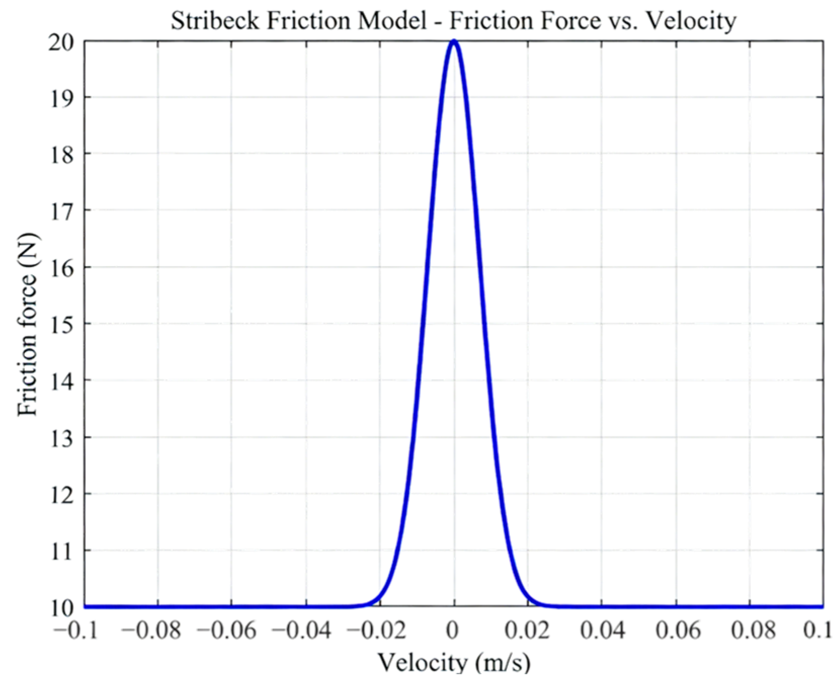
The Stribeck friction model is currently the most widely used cylinder friction model in position control systems. The formula for this substance is as follows:

$$F_{v }={ F}_{\mathrm{c}} + \left(F_{\mathrm{s} }-F_{\mathrm{c}}\right)e^{-{\left({\displaystyle \frac{v}{v_s}}\right)}^{\delta }}\mathit{sgn}(v) +{ C}_v$$

(5)

The fifth equation indicates that F_s represents the static friction force, F_c signifies the Coulomb friction force, v denotes the piston velocity, µs characterizes the Stribeck separation velocity, and δ is an undetermined coefficient ranging from 0.5 to 2.

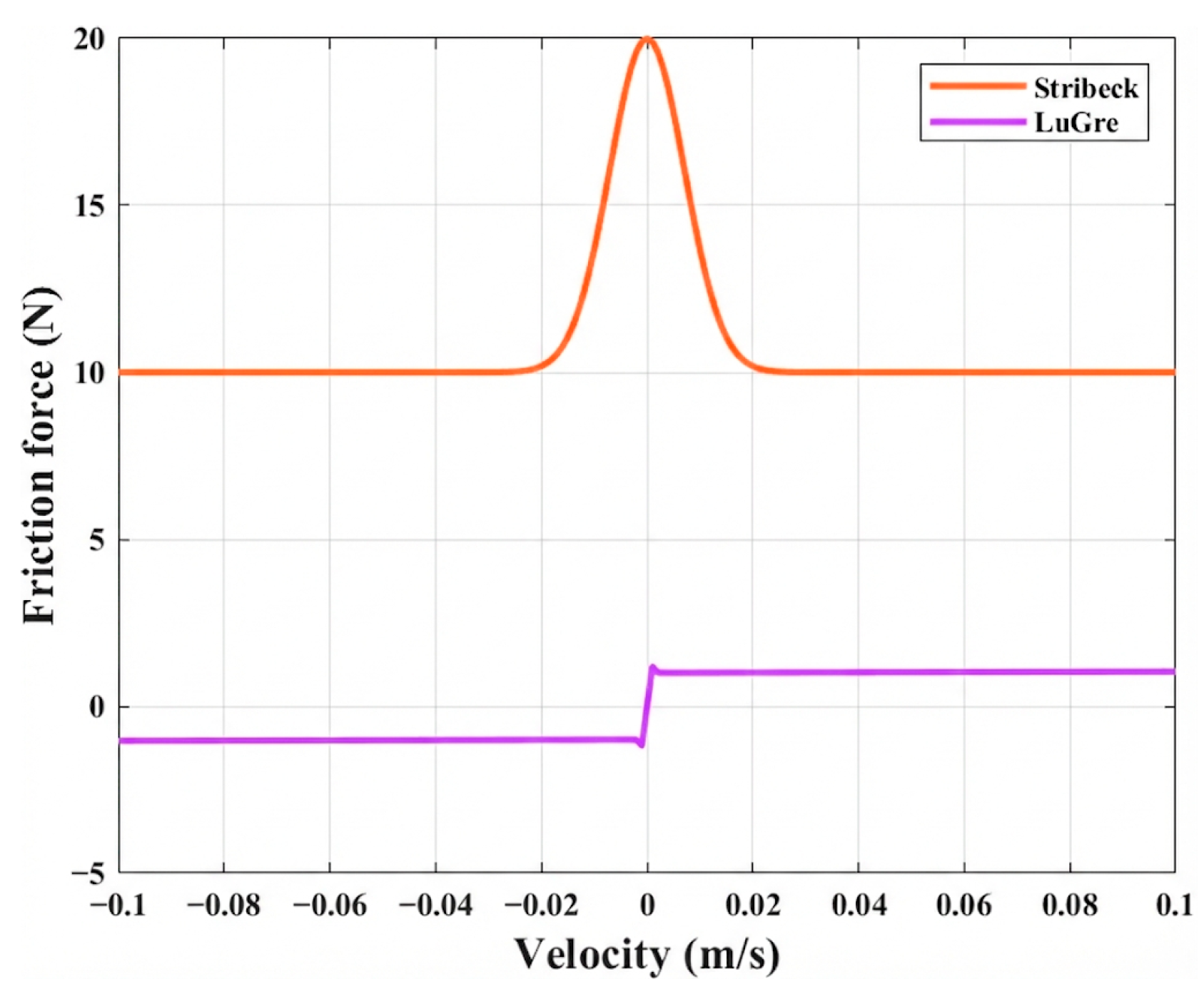
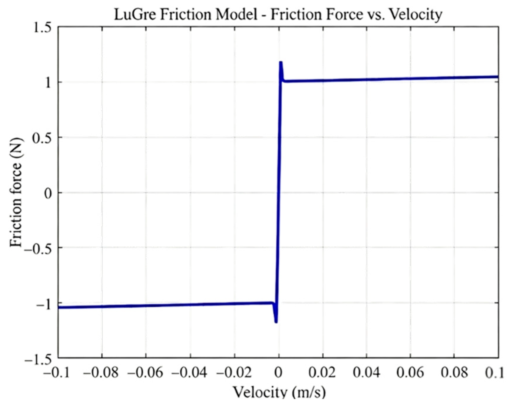
The Stribeck friction model is a useful tool for understanding the behavior of friction forces at low speeds. It expresses the negative slope friction phenomenon through a decaying exponential term, as illustrated in Figure 1. However, it is important to note that the Stribeck model does not account for nonlinear factors such as friction hysteresis and varying critical friction forces. When the velocity of the object crosses zero, the friction force undergoes a sudden change in magnitude. In a force-controlled system, the variable directly affected is the force. A sudden change in friction force results in an abrupt change in the force response, leading to high-frequency oscillations in the system. However, these oscillations do not align with real-world conditions. In reality, friction force also exhibits time-dependent behavior, known as friction memory. Friction memory is defined as the phenomenon in which friction force lags behind the change in relative velocity between contacting surfaces. The LuGre model effectively accounts for this factor by incorporating friction memory characteristics, thereby preventing high-frequency oscillations, as illustrated in Figure 2.

The LuGre model conceptualizes the friction contact surface as a set of elastic bristles exhibiting random behavior at the microscopic level. The generation of friction force is attributed to the bending of these bristles, as depicted in the subsequent formula:

$$F = {\sigma }_{0}z + {\sigma }_1{\displaystyle \frac{\mathrm{d}z}{\mathrm{d}t}} + {\sigma }_{2}v$$

(6)

$${\displaystyle \frac{\mathrm{d}z}{\mathrm{d}t}} =v -{\displaystyle \frac{\left|v\right|}{g\left(v\right)}}$$

(7)

$${\sigma }_{0}g(v)=F_{\mathrm{c}} +(F_{\mathrm{s}}-F_{\mathrm{c}})e^{-{\left({\displaystyle \frac{v}{v_{\mathrm{s}}}}\right)}^2}$$

(8)

In Equations (6)–(8), v represents the relative velocity of the friction surfaces, z denotes the relative deformation between the moving surfaces under viscous conditions, ${\sigma }_0$ is the stiffness of the microscopic deformation z before movement, ${\sigma }_1$ is the dynamic damping of dz/dt, and ${\sigma }_2$ is the viscous friction coefficient.

Consequently, the LuGre model is employed in this simulation. The model accounts for the negative slope of the Stribeck velocity and also reflects nonlinear characteristics such as pre-sliding displacement, friction hysteresis, varying critical friction force, and viscous sliding. This model is currently regarded as one of the most comprehensive and accurate models available, as illustrated in Figure 3.

2.2. Multiphysics Coupling Model

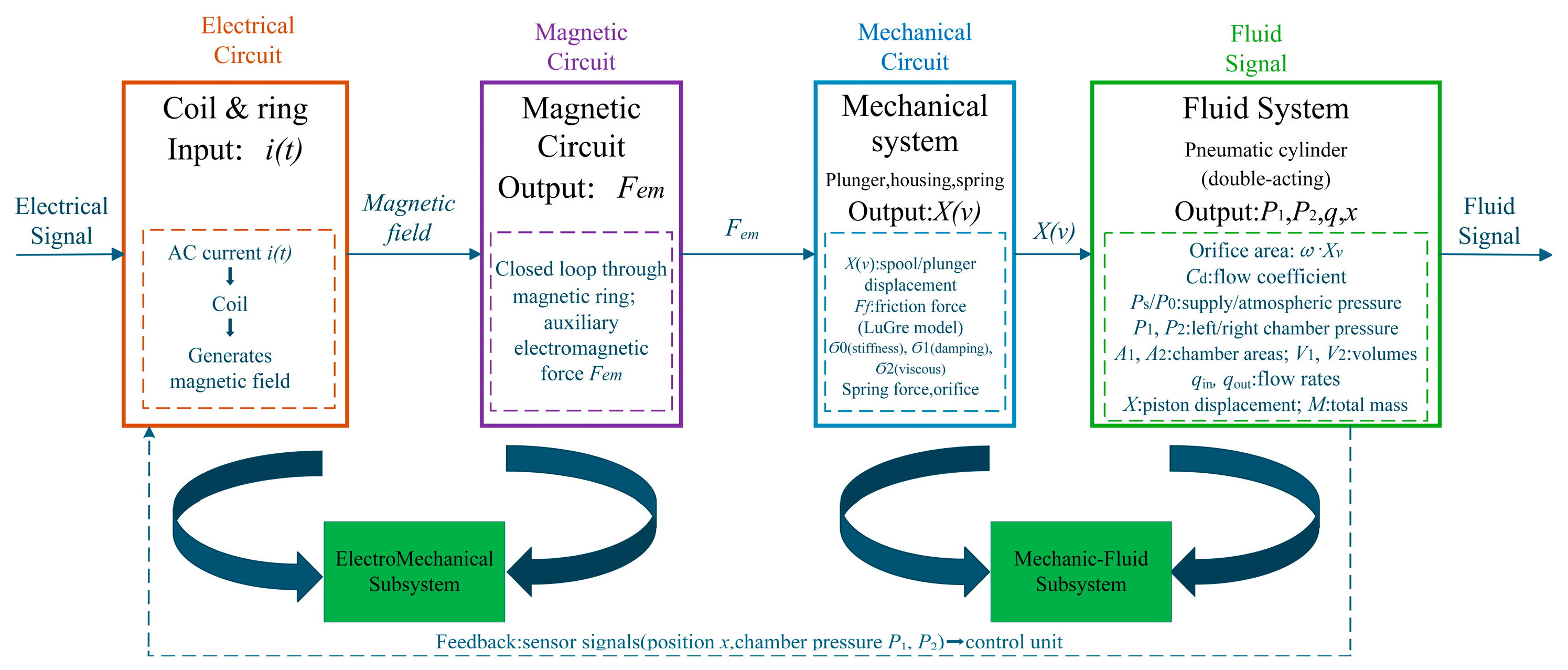
The solenoid valve utilized in this study is composed of a coil, an orifice, a ring, a plunger housing, and a spring. When the coil is connected to a power supply, alternating current is conducted through the windings, thereby generating a magnetic field. This magnetic field tends to form a closed loop through the magnetic ring along a path that minimizes magnetic reluctance. As a result, the plunger slides toward the plunger housing under the influence of the spring force. In practical operation, the force generated due to various resistances may be insufficient to overcome the spring force and thus fail to induce the sliding of the plunger. Therefore, an additional magnetic field is generated from the magnetic ring, which interacts with the main magnetic field to produce an auxiliary electromagnetic force.

The valve model comprises four distinct subsystems: an electrical system, a magnetic system, a mechanical system, and a fluid system (see Figure 4).

2.2.1. Pressure Differential Equation

In accordance with the law of conservation of mass, under the assumption that the working medium is continuous, the storage rate of mass stored in a control body is equivalent to the mass flow rate minus the mass flow rate:

$$\Sigma {\dot{M}}_{\mathrm{in}} - \Sigma {\dot{M}}_{\mathrm{out}} = {\displaystyle \frac{\mathrm{d}u}{\mathrm{d}t}} = {\displaystyle \frac{\mathrm{d}\left(\rho v\right)}{\mathrm{d}t}} = \rho {\displaystyle \frac{\mathrm{d}v}{\mathrm{d}t}} + v{\displaystyle \frac{\mathrm{d}\rho }{\mathrm{d}t}}$$

(9)

Substituting the gas equation into the aforementioned equation and simplifying, we obtain:

$${\displaystyle \frac{\mathrm{d}M}{\mathrm{d}t}} = {\displaystyle \frac{1}{\mathrm{R}T}}\left(P{\displaystyle \frac{\mathrm{d}v}{\mathrm{d}t}} + {\displaystyle \frac{v}{k}}{\displaystyle \frac{\mathrm{d}p}{\mathrm{d}t}}\right)$$

(10)

Assuming $\mathrm{T}1 = \mathrm{T}2 = \mathrm{T}$ and disregarding the effect of temperature changes, substitute the parameters of the two chambers of the cylinder into the aforementioned formula to obtain: Substituting the gas equation into the aforementioned equation and simplifying, we obtain:

$${\displaystyle \frac{{\mathrm{d}p}_1}{\mathrm{d}t}} = {\displaystyle \frac{K(\mathrm{R}T{Q}_{\mathrm{m}1} - P_1{A}_1\frac{\mathrm{d}x}{\mathrm{d}t})}{V_1}}$$

(11)

$${\displaystyle \frac{{\mathrm{d}p}_2}{\mathrm{d}t}}={\displaystyle \frac{K(\mathrm{R}T{Q}_{\mathrm{m}2}-P_2{A}_2\frac{\mathrm{d}x}{\mathrm{d}t})}{V_2}}$$

(12)

In Equations (11) and (12), $A_1$ and $A_2$ denote the left and right chamber areas of the pneumatic cylinder, respectively. $V_1$ and $V_2$ represent the volumes of the left and right chambers of the cylinder, respectively. $Q_{\mathrm{m}1}$ and $Q_{\mathrm{m}2}$ represent the flow rates entering and exiting the left and right chambers of the cylinder, respectively. $x$ represents the piston displacement of the cylinder.

2.2.2. Force Equilibrium Equations in Fluid Systems

In accordance with Newton’s second law, the force balance equation for the cylinder is expressed as follows:

$$P_1{A}_1 - P_2{A}_2-F_{\mathrm{f}} = m{\displaystyle \frac{{\mathrm{d}}^{2}y}{\mathrm{d}{t}^2}} + \mathit{ky} + F$$

(13)

In Equation (13), $F_{\mathrm{f}}$ denotes the friction force exerted on the cylinder, $F$ signifies the external load force acting on the cylinder, $m$ represents the total mass of the moving components and the load on the cylinder, and $k$ represents the spring stiffness of the load.

2.2.3. Pneumatic System Modeling

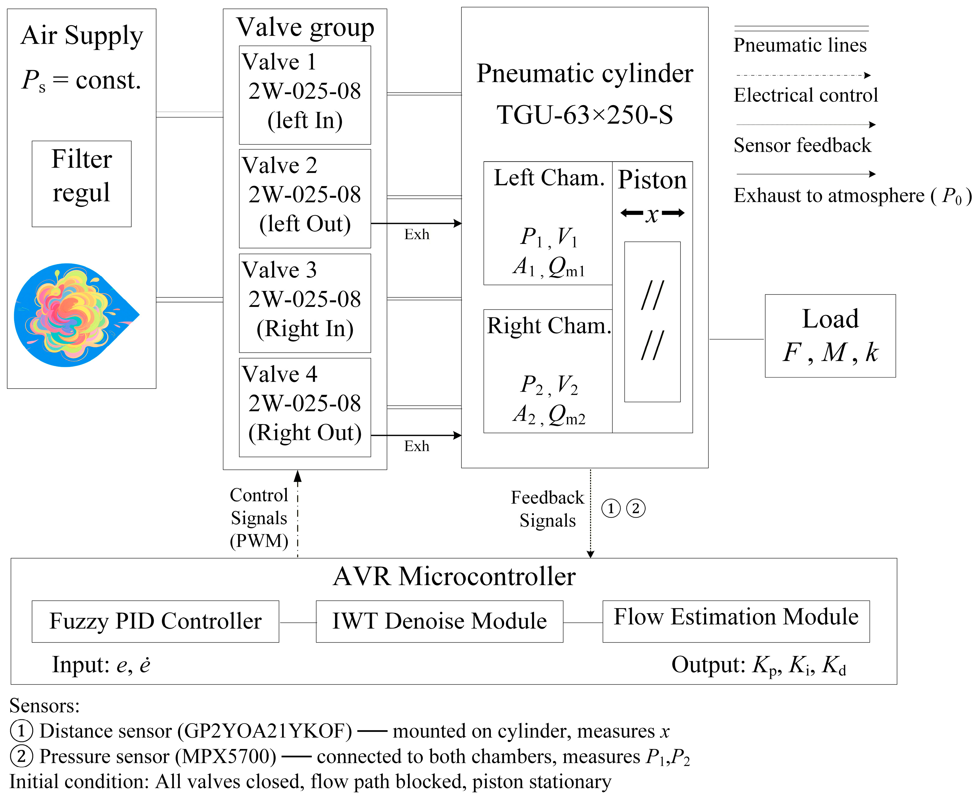
As illustrated in Figure 5, the experimental setup of the electric-pneumatic system was designed to test the effectiveness of the proposed method. The effectiveness of the system is contingent upon the configuration of the valves [24]. The experimental setup, as illustrated in Figure 5, incorporates components sourced from various manufacturers. The control unit is built around an AVR microcontroller; however, the specific manufacturer and origin of this component were not detailed in the referenced sources. The pneumatic actuators consist of double-acting cylinders (model TGU-63×250-S, stroke 250 mm, piston diameter 63 mm), for which manufacturer information could not be determined. The system employs four 2-2 quick-change valves (model 2W-025-08); these valves are commonly produced by manufacturers such as Zhaoqing Hongsheng Coating Machinery Parts Co., Ltd. (Foshan, China) and Baodelong Instrument Factory (Zhejiang, China). Position feedback is provided by a distance sensor (model GP2YOA21YKOF) manufactured by Sharp Corporation (Osaka, Japan). Pressure measurements in the cylinder chambers are obtained using a pressure sensor (model MPX5700) supplied by NXP Semiconductors (Eindhoven, The Netherlands). The valves are closed under initial conditions, thus closing the flow path and keeping the piston stationary. As illustrated in Figure 5, the position sensor and pressure sensor provide data on the piston position and chamber pressure to the control unit.

2.2.4. Description of Experimental Equipment Parameters and Environmental Conditions

In order to enhance the reproducibility of the experiment, this paper provides supplementary explanations on the key parameters and environmental conditions of the experimental device. The main parameters of the experimental system are shown in

Table 1. Experimental Parameters.

Category	Parameter	Symbol	Value	Unit	Description
Air Supply System	Supply Pressure	P_s	0.6	MPa	Stable compressed air source
Air Supply System	Pressure Fluctuation	ΔP	±0.01	MPa	Ensures system stability
Sensor	Pressure Sensor Range	-	0–1.0	MPa	Measurement range
Sensor	Pressure Sensor Accuracy	-	±0.25%	FS	Full-scale accuracy
Sensor	Displacement Sensor Resolution	-	0.01	mm	High-precision displacement detection
Controller	Control Algorithm	-	Fuzzy PID	-	Adaptive control strategy
Controller	Sampling Time	T_s	1	ms	Real-time control interval
Environment	Ambient Temperature	T	25 ± 2	°C	Laboratory condition
Environment	Relative Humidity	RH	50 ± 5%	%	Controlled humidity
Environment	Vibration Level	-	<0.05	g	Low vibration platform
Test Object	Load Range	-	0–500	N	External disturbance simulation
Test Object	Actuator Type	-	Electro-pneumatic actuator	-	Experimental actuator

. The air source pressure is stable at 0.6 MPa, and the pressure fluctuation does not exceed ±1.5%. The experimental environment temperature was maintained at 25 ± 2 °C, and the relative humidity was approximately 45–55%.

The displacement sensor adopts GP2YOA21YKOF, with a measuring range of 10–80 cm and a resolution of about 1 mm; the pressure sensor adopts MPX5700, with a range of 0–700 kPa, and the nonlinear error is less than ±0.25%. The sampling frequency is set to 1 kHz, and the data is collected by the AVR controller and transmitted to the upper computer for processing.

3. Fuzzy PID Controller Design

Having established the multi-physics coupling model of the proportional valve system in Section 2, this section addresses the design of the fuzzy PID controller that operates on the estimated flow signal to dynamically compensate for the plant nonlinearities identified above.

3.1. Control Objectives and Structure

In order to address the parameter time-varying issue caused by the nonlinearity of the proportional valve, the employment of fuzzy control rules has been proposed to modify the PID parameters online. This modification constitutes a fuzzy self-tuning PID controller [25,26], the structure of which is shown in Figure 6. The establishment of a fuzzy inference mechanism is based on the performance requirements of the electromagnetic pneumatic system. The purpose of this establishment is twofold: first, to eliminate the influence of unmodeled dynamic characteristics, and second, to enhance the robustness of the controller. The fuzzy inference component is responsible for monitoring the waveform of the control response in real time to calculate performance metrics such as rise time, overshoot, and steady-state error.

3.2. Setting Fuzzy Language Variables

The system deviation e and the deviation change rate $\dot{e}$ are utilized as input language variables for the fuzzy controller, while the parameters $K_{\mathrm{p}}$, $K_{\mathrm{i}}$ and $K_{\mathrm{d}}$ are employed as output language variables. The variation in these systems is defined by the fundamental domains of fuzzy sets:

$$e,\dot{e},{ K}_{\mathrm{p}}{,{ K}_{\mathrm{i}}, K}_{\mathrm{d}} = (-4, -3, -2, -1, 0, 1, 2, 3, 4)$$

(14)

Its fuzzy subset is denoted by $\mathrm{e},\dot{\mathrm{e}}=\left\{\mathrm{N}\mathrm{B},\mathrm{N}\mathrm{S},\mathrm{Z}\mathrm{E},\mathrm{P}\mathrm{S},\mathrm{P}\mathrm{B}\right\}$, and the elements in the subset represent negative large, negative small, zero, positive small, and positive large, respectively.

The continuously varying quantities within the basic domain are to be divided into discrete levels, followed by the implementation of fuzzy processing. The range of variation for the speed deviation e and the deviation change rate e of the secondary element is specified as [−4, 4]. In the event that the values fall outside this interval, they can be converted to the range [−4, 4] using the linear transformation Formula (15).

$$y ={\displaystyle \frac{8}{b - a}}(x - {\displaystyle \frac{a+b}{2}})$$

(15)

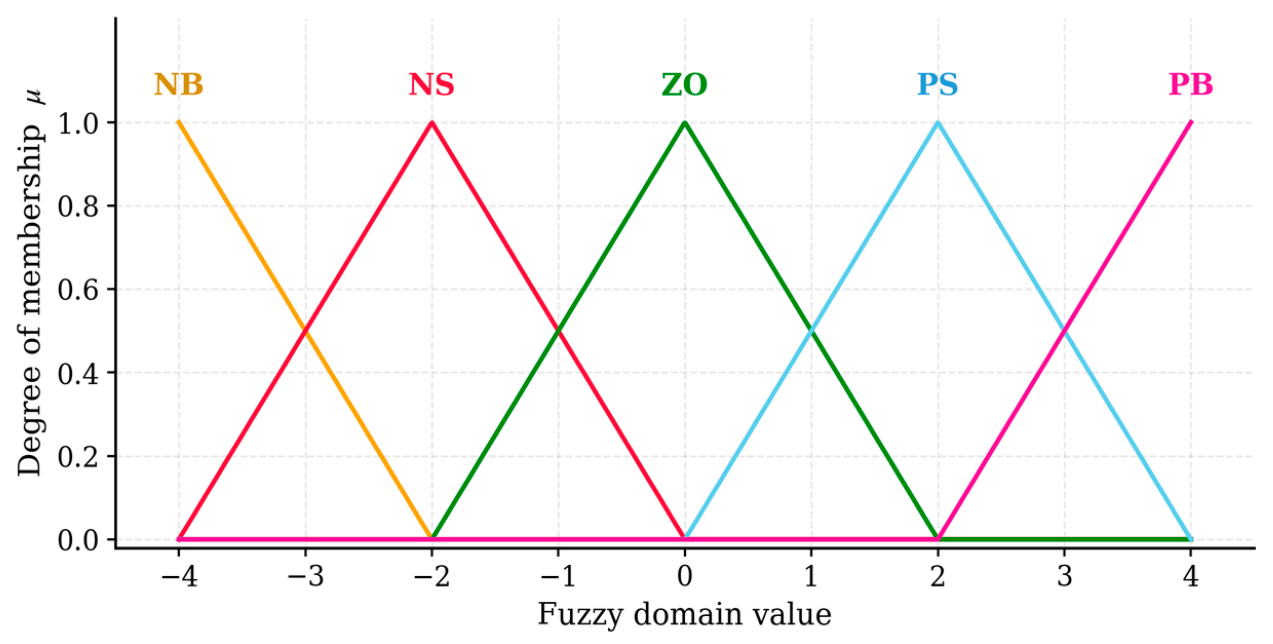
The membership functions employed for each fuzzy state are typically selected from a range of options, including symmetric triangular, symmetric trapezoidal, and normal-type functions. The underlying reason for this phenomenon is that the configuration of a triangular membership function is contingent upon the gradient of its corresponding straight line. This attribute of the function renders the computational process more straightforward and reduces the requirement for memory storage. Consequently, it is especially well-suited for fuzzy control systems in which membership functions must be adjusted in real time. In such scenarios, a triangular membership function is chosen for the language variable, as illustrated in Figure 7.

Indeed, the configuration of the membership function-whether triangular, trapezoidal, or of a normal distribution, among others-exerts minimal influence on the control performance. Conversely, the extent of each fuzzy subset’s coverage over the entire domain demonstrates a substantial impact on performance. Consequently, the membership functions previously employed are still applicable. Consequently, the assignment tables for the membership degrees $e,\dot{e}$, and $K_{\mathrm{p}}{, K_{\mathrm{i}}, K}_{\mathrm{d}}$ can be determined.

3.3. Fuzzy Rules

Control rules constitute the fundamental components of fuzzy controllers. A substantial body of research has been dedicated to the development of effective control strategies, which are then refined through a process of organization, processing, and refinement. These strategies are described using the fuzzy states of input and output variables to establish control rules.

The output parameters of the PID controller are represented by the following formulas:

$$K_{\mathrm{p}}^{\prime } = {\displaystyle \frac{K_{\mathrm{p}} - K_{\mathrm{p},\min }}{K_{\mathrm{p},\max } - K_{\mathrm{p},\min }}}$$

(16)

$$K_{\mathrm{i}}^{\prime }={\displaystyle \frac{K_{\mathrm{i}}-K_{\mathrm{i},\min }}{K_{\mathrm{i},\max }-K_{\mathrm{i},\min }}}$$

(17)

$$K_{\mathrm{d}}^{\prime }={\displaystyle \frac{K_{\mathrm{d}}-K_{\mathrm{d},\min }}{K_{\mathrm{d},\max }-K_{\mathrm{d},\min }}}$$

(18)

The range of the error and the error change in a fuzzy controller is referred to as the basic domain of these variables. In order to execute the process of fuzzy processing, it is necessary to transform the basic domains of the input error and error change into the domains of the corresponding fuzzy sets. This transformation requires the application of a quantization factor. Concurrently, the range of control quantity changes required by the controlled object is referred to as the basic domain of the input quantity. When transferring the control quantity obtained from the fuzzy control algorithm to the basic domain, it is imperative that the quantity be multiplied by a proportionality factor. The following variables are introduced: the error and error rate input quantization factors $K_e$ and $K_{\mathrm{e}\mathrm{c}}$, as well as the output transformation proportionality factor $K_{\mathrm{u}}$.

The input quantization factors $K_{\mathrm{e}}$ and $K_{\mathrm{e}\mathrm{c}}$, as well as the output transformation ratio factor $K_{\mathrm{u}}$, have been demonstrated to have a significant impact on the dynamic and static performance of the system. Therefore, it is imperative that they be selected with precision. The input quantization factor is contingent upon the maximum overshoot in the response curve, while the output ratio factor is influenced by the initial PID parameters and is also associated with the desired response performance.

$$R_l =e,\dot{e} \to K_{\mathrm{p}} ={\int }_{e\times \dot{e}\times K_{\mathrm{p}}} {\displaystyle \frac{\mu (e)\Lambda \mu (\dot{e})\Lambda \mu \left(K_{\mathrm{p}}^{\prime }\right)}{(e,\dot{e},K_{\mathrm{p}}^{\prime })}}$$

(19)

In order to ensure the rationality and repeatability of fuzzy PID controller parameter tuning, this paper systematically explains the selection of error quantization factor $K_{\mathrm{e}}$, error change rate quantization factor $K_{\mathrm{e}\mathrm{c}}$ and output scale factor $K_{\mathrm{u}}$.

Among them, $K_{\mathrm{e}}$ and $K_{\mathrm{e}\mathrm{c}}$ are mainly used to map the actual error and error change rate to the fuzzy universe, and their values are determined according to the maximum steady-state error and the maximum error change rate in the system step response; $K_{\mathrm{u}}$ is used to reflect the fuzzy reasoning results into the actual PID parameter adjustment amplitude, and their initial values are obtained according to the Ziegler-Nichols critical proportion method.

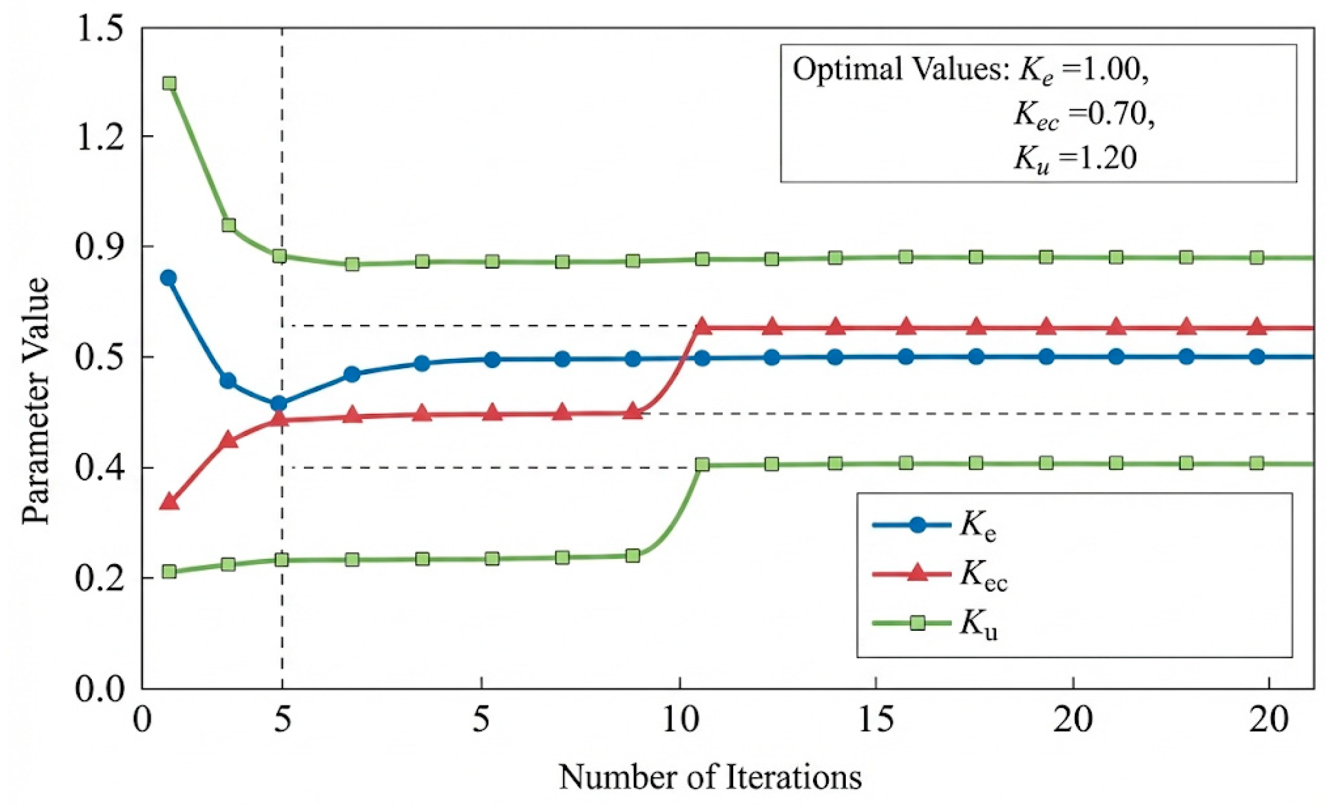
On this basis, this paper further uses the parameter sensitivity analysis method to simulate $K_{\mathrm{e}}$, $K_{\mathrm{e}\mathrm{c}}$ and $K_{\mathrm{u}}$ within a variation range of ± 20%. Taking the overshoot, adjustment time and steady-state error as evaluation indicators, the optimal parameter combination is finally determined. The results show that this parameter configuration ensures rapid response of the system while significantly suppresses the oscillation caused by friction nonlinearity. The sensitivity analysis of fuzzy PID parameters is shown in

Table 2. Parameter sensitivity analysis.

${\mathit{K}}_{\mathbf{e}}$ Rate of Change	${\mathit{K}}_{\mathbf{e}\mathbf{c}}$ Rate of Change	${\mathit{K}}_{\mathbf{e}}$ Rate of Change	The Overshoot (%)	Adjustment Time (s)	Steady State Error (mm)	Evaluation
−20%	−20%	−20%	7.8	0.92	0.48	Slow response and weak control
−10%	−10%	−10%	6.1	0.78	0.32	Improved performance
0	0	0	4.2	0.63	0.18	Optimal parameter combination
+10%	+10%	+10%	4.9	0.66	0.21	Slightly oscillating but acceptable
+20%	+20%	+20%	6.7	0.81	0.36	Increased oscillation and decreased stability

. The parameter optimization process is given, as shown in Figure 8.

We note that the sensitivity analysis presented in Table 2 adopts a simultaneous perturbation approach, in which all three parameters ($K_{\mathrm{e}}, K_{\mathrm{ec}},{ K}_{\mathrm{u}}$) are varied by the same percentage simultaneously. This choice was made for the following reasons:

(1) Physical coupling: In the fuzzy PID framework, the three quantization/scaling factors are not independent design variables but are functionally coupled through the fuzzy inference process. Specifically, $K_{\mathrm{e}}$ and $K_{\mathrm{ec}}$ jointly determine the operating point within the fuzzy rule table, while ${ K}_{\mathrm{u}}$ scales the output. Perturbing one factor while fixing the others may yield misleading sensitivity indices because the fixed factors would no longer correspond to their optimal values for the perturbed system.

(2) Worst-case robustness: Simultaneous perturbation represents the most conservative (worst-case) scenario for parameter uncertainty, as all parameters deviate from their nominal values at the same time. If the system maintains satisfactory performance under this condition, it is guaranteed to perform at least as well under any single-factor perturbation of the same magnitude.

(3) Practical relevance: In real-world deployment, parameter deviations due to component aging, environmental changes, or calibration errors tend to affect multiple parameters simultaneously rather than in isolation.

The results in Table 2 demonstrate that the system performance degrades gracefully under simultaneous perturbation of up to ±20%, with overshoot remaining below 7.8% and steady-state error below 0.48 mm. This provides strong evidence of robustness for practical applications.

The total fuzzy relationship between, $K_{\mathrm{p}}$, $K_{\mathrm{i}}$, and $K_{\mathrm{d}}$ is as follows:

$$\left\{\begin{array}{c}{R}_{K_{\mathrm{p}}}= {\displaystyle \bigcup _{l = 1}^{25}}{R}_l\\ R_{K_{\mathrm{i}}} = {\displaystyle \bigcup _{m = 1}^{25}}{R}_m\\ R_{K_{\mathrm{d}}} = {\displaystyle \bigcup _{n = 1}^{25}}{R}_n\end{array}\right.$$

(20)

In the formula:

$$\left\{\begin{array}{c}{R}_m = e,\dot{e} \to { K}_{\mathrm{i} }= {\int }_{e\times \dot{e}\times K_{\mathrm{i}}} {\displaystyle \frac{\mu \left(e)\Lambda \mu \right(\dot{e})\Lambda \mu \left(K_{\mathrm{i}}^{\prime }\right)}{(e,\dot{e},K_{\mathrm{i}}^{\prime })}}\\ R_n = e,\dot{e} \to K_{\mathrm{d} }= {\int }_{e\times \dot{e}\times K_{\mathrm{d}}} {\displaystyle \frac{\mu \left(e)\Lambda \mu \right(\dot{e})\Lambda \mu \left(K_{\mathrm{d}}^{\prime }\right)}{(e,\dot{e},K_{\mathrm{d}}^{\prime })}}\end{array}\right.$$

(21)

The core principle of fuzzy PID control lies in employing fuzzy rules to dynamically adjust controller parameters. In electromagnetic pneumatic systems, primary nonlinearities stem from the LuGre friction model’s memory effect, flow equation pressure dependence, and dynamic cylinder load disturbances. Rule table design integrates these nonlinear characteristics with system dynamics and empirical knowledge. When the error ($e$) and error rate ($\dot{e}$) belong to different fuzzy states, $K_{\mathrm{p}}$, $K_{\mathrm{i}}$, and $K_{\mathrm{d}}$ are adaptively tuned to enhance control performance. For significant negative displacement errors, $K_{\mathrm{p}}$ is set to “positive large (PB)” to correct steady-state error quickly, $K_{\mathrm{i}}$ is gradually increased to accelerate convergence, while $K_{\mathrm{d}}$ is reduced to avoid high-frequency oscillations caused by friction memory. As the valve spool nears the target, all gains converge to “zero (ZE),” ensuring smooth transitions and minimizing overshoot from pressure fluctuations. In overshoot scenarios, $K_{\mathrm{p}}$ switches to “negative large (NB)” for rapid correction, and $K_{\mathrm{d}}$ is increased to mitigate inertial effects from sudden load changes. When the error rate $\dot{e}$ crosses zero, $K_{\mathrm{d}}$ is set to “positive small (PS),” enhancing differential action to compensate for bristle deformation dynamics in the LuGre model and suppress oscillations. Finally, fuzzy outputs are defuzzified into precise control signals.

3.4. Defuzzification

The results of fuzzy reasoning, that is to say, the output variables of the fuzzy controller, are generally fuzzy sets that cannot be directly used to control the controlled object. The initial step involves the conversion of the variables into precise quantities that can be executed by the actuator. This process is commonly referred to as defuzzification, and the center of gravity method is a widely used defuzzification method in fuzzy control systems.

The variable z is the center of the area covered by the membership function of the fuzzy set:

$$z^{\ast } = {\displaystyle \frac{{\int }_a^{b}z{\mu }_{\mathrm{c}}\left(z\right)\mathrm{d}z}{{\int }_a^b{\mu }_c\left(z\right)\mathrm{d}z}}, U = [a,b]$$

(22)

It is imperative to acknowledge that the precise values of the output variables obtained through defuzzification are exclusively the exact values within their respective domains. Furthermore, contingent on the domain of the output variable and the fuzzy state, the domain-specific exact value of the output variable must undergo conversion back to its corresponding actual exact value through the inverse process of converting the actual exact value of the input variable into a domain-specific exact value. The resulting precise value of the output variable can then be used as the exact quantity that the fuzzy controller transmits to the actuator for control of the controlled object.

3.5. Stability and Parametric Disturbance Analysis

In essence, fuzzy PID controllers can be regarded as a kind of time-varying PID controllers whose parameters are adjusted online. Under the conditions of small system errors and stable operating points, the fuzzy inference output tends to be constant, and the controller is equivalent to a linear PID structure. At this time, the system stability can be analyzed with reference to the classic PID closed-loop stability conditions.

To provide a formal stability argument, we adopt the framework of Lyapunov-based analysis for bounded-parameter time-varying systems. Define the Lyapunov function candidate as

$$V (e) = {\displaystyle \frac{1}{2}}{ e}^2$$

(23)

where $e$ denotes the tracking error. The time derivative along the closed-loop trajectory yields:

$$\dot{V } = e·\dot{e}$$

(24)

Under fuzzy PID control, the control output is expressed as

$$u=K_{\mathrm{p}}·e+K_{\mathrm{i}}\cdot \int \mathit{edt} +K_{\mathrm{d}}\cdot \dot{e}$$

(25)

where $K_{\mathrm{p}}$, $K_{\mathrm{i}}$, $K_{\mathrm{d}}$ are online-tuned by the fuzzy inference engine. The key structural property is that the fuzzy rule base confines the PID gains within predetermined bounds:

$$\left\{\begin{array}{c}{K}_{\mathrm{p}}\in \left[K_{\mathrm{p},\min }, K_{\mathrm{p},\max }\right]\\ K_{\mathrm{i}}\in \left[K_{\mathrm{i},\min }, K_{\mathrm{i},\max }\right]\\ K_{\mathrm{d}}\in \left[K_{\mathrm{d},\min }, K_{\mathrm{d},\max }\right]\end{array}\right.$$

(26)

These bounds are explicitly enforced by the fuzzy universe boundaries (range [−4, 4] as defined in Section 3.2) and the output scaling factor $K_{\mathrm{u}}$. Within this bounded parameter set, for any admissible combination ($K_{\mathrm{p}}{, K_{\mathrm{i}}, K}_{\mathrm{d}}$), the equivalent linear PID controller satisfies the Routh–Hurwitz stability criterion for the linearized plant model derived. Consequently, $\dot{V}<0$ for all $e\ne 0$ within the operating region, guaranteeing local asymptotic stability.

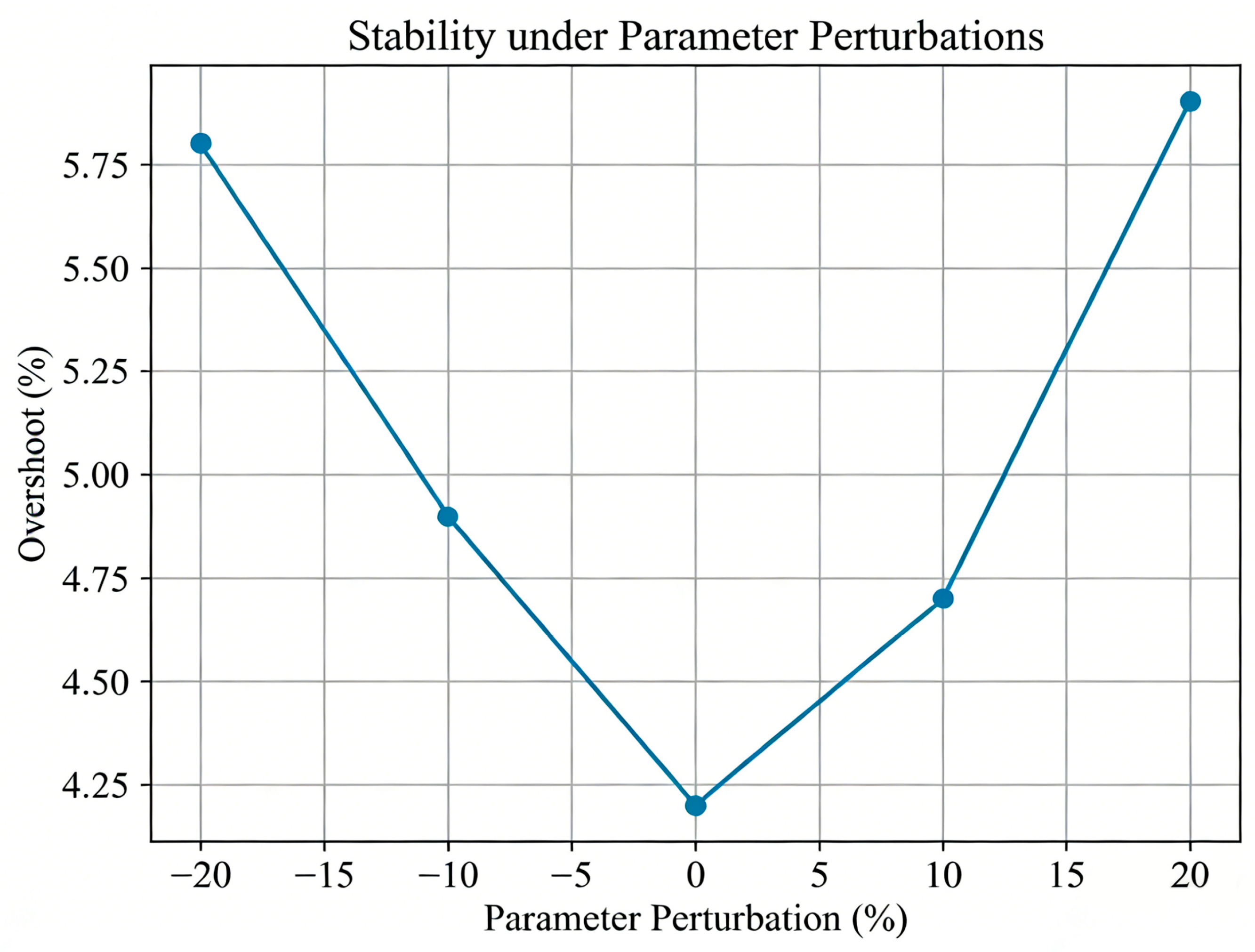
Furthermore, since the fuzzy rule adjustment is memoryless (i.e., the parameter update at each instant depends only on the current $e$ and $\dot{e}$, not on past values), the closed-loop system can be modeled as a linear parameter-varying (LPV) system with polytopic uncertainty. The stability of such systems is guaranteed if a common Lyapunov function exists for all vertex controllers—a condition satisfied here because the Routh–Hurwitz conditions hold for all four corner points of the ($K_{\mathrm{p}}{, K_{\mathrm{i}}, K}_{\mathrm{d}}$) parameter box. The simulation results presented in

Table 3. Parameter perturbation stability analysis of fuzzy PID.

Parameter Perturbation	Overshoot (%)	Settling Time (s)	Steady-State Error (mm)	Stability Judgment
−20%	5.8	0.74	0.29	Stable
−10%	4.9	0.68	0.22	Stable
0% (Nominal)	4.2	0.63	0.18	Optimal and Stable
+10%	4.7	0.66	0.20	Stable
+20%	5.9	0.79	0.31	Stable with slight oscillation

and Figure 9 confirm this theoretical prediction: the system remains asymptotically stable under ±20% parameter perturbation with bounded overshoot (≤5.9%) and settling time (≤0.79 s).

We acknowledge that a rigorous global stability proof for the full nonlinear system (incorporating the LuGre friction model and compressible flow dynamics) would require advanced tools such as integral quadratic constraints (IQCs) or sum-of-squares (SOS) programming, which is beyond the scope of the current work. Nevertheless, the Lyapunov-based local analysis, combined with the extensive simulation validation, provides sufficient evidence of robust stability for the operating conditions considered in this study.

When system parameters are disturbed, fuzzy rules adjust the amplitude by limiting PID parameters to avoid closed-loop instability caused by sudden changes in parameters. Simulation results show that within the range of ±20% parameter disturbance, the system response remains asymptotically stable, and there is no divergence or continuous oscillation, indicating that the proposed control strategy has certain robust stability. As shown in Table 3. The stability parameter disturbance response is shown in Figure 9.

4. Improved Application of Wavelet Threshold Denoising in Flow Estimation of Proportional Control Valves

The fuzzy PID controller designed in Section 3 relies on accurate flow feedback. However, sensor signals in the pneumatic system are corrupted by high-frequency electromagnetic noise and low-frequency pressure drift. This section presents an improved wavelet threshold (IWT) denoising technique to provide clean feedback signals.

4.1. Improvement of the Wavelet Threshold Denoising Principle and Noise Characteristic Analysis

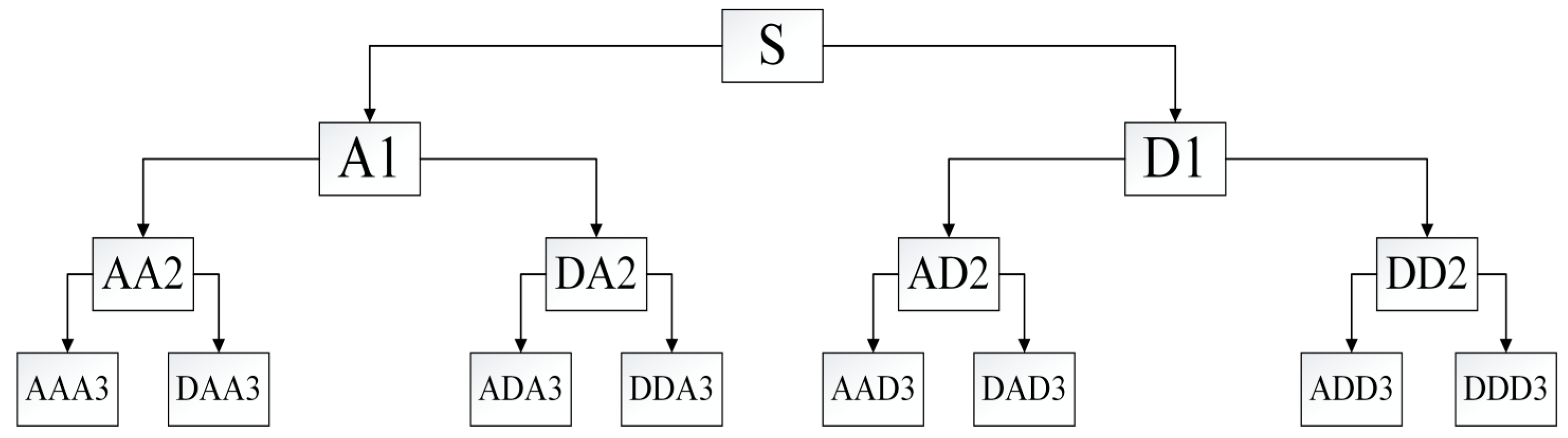
Sensors in pneumatic systems are often subject to high-frequency noise signals due to the presence of high-frequency vibrations and electromagnetic interference caused by external components. In this study, an enhanced wavelet threshold denoising technique was employed to eliminate noise. The enhanced wavelet threshold denoising technique is a filtering method based on wavelet transform [27,28,29], which employs a tree-structured embedding algorithm to decompose and calculate the noisy signal layer by layer, as illustrated in Figure 10 [30] (where S is the original signal, cA₁ and cD₁ represent the high-frequency and low-frequency signals, respectively). Subsequently, the decomposed frequency bands are further divided into high and low halves to match the signal spectrum, thereby achieving a more refined decomposition. The denoised signal is obtained by selecting an appropriate number of layers and wavelet bases to decompose the noise signal, selecting an appropriate threshold to quantize each layer, and finally reconstructing the wavelet coefficients.

4.2. Adaptive Threshold Function Design

The improved wavelet threshold function expression is as follows, based on the characteristics of the flow signal of the proportional control valve:

$$W_n=\left\{\begin{array}{c}{\omega }_n\sin \left({\displaystyle \frac{\pi }{2}}u\right)\xi {\mathrm{e}}^u, \left|{\omega }_n\right|\ge {\lambda }_n\\ \mathrm{s}\mathrm{i}\mathrm{g}\mathrm{n}\left({\omega }_n\right){\lambda }_n\xi {\mathrm{e}}^u,\left|{\omega }_n\right|<{\lambda }_n\end{array}\right.$$

(27)

where ω_n is the wavelet coefficient of the original signal decomposed at the nth layer; λ_n is the threshold value for the wavelet coefficients at each layer. When $\left|{\omega }_n\right|\ge {\lambda }_n$, to simulate the real environment, a decaying sine function is used for noise reduction; when $\left|{\omega }_n\right|<{\lambda }_n$, the noise ratio is relatively high, so an exponential noise reduction method is adopted.u is the threshold function adjustment factor, determined by calculating the average and standard deviation of the wavelet coefficients, then adding or subtracting one multiple of the standard deviation from the average. Its range is (0, 1], and ξ is a constant of 0.02. The decaying sine function is used to balance detail preservation and noise reduction requirements.

The vibration signal, herein designated as $x\left(t\right)$, is subjected to wavelet decomposition. The threshold calculation formula [31] corresponding to each layer of wavelet coefficients is as follows:

$${\lambda }_n={\displaystyle \frac{{\sigma }_n\sqrt{2\mathit{ln}N}}{n^2}}, n = 1, 2, 3, \dots$$

(28)

where σ_n is the noise standard deviation of the nth wavelet coefficient; N is the signal length, and ${\sigma }_n$ is defined in [32] as follows:

$${\sigma }_n=\sqrt{{\displaystyle \frac{\mathrm{median}(\left|{\omega }_n\right|)}{0.6745}}}$$

(29)

As the decomposition scale increases, the threshold decreases, thereby satisfying the characteristic that the wavelet coefficient of vibration signals decreases as the decomposition scale increases. This results in better noise reduction.

4.3. Convergence and Boundedness Analysis

For the fuzzy rule adjustment process, since the adjustment range of PID parameters is limited by the boundary of the fuzzy universe, the system output always remains bounded, avoiding the problem of parameter divergence.

The boundedness of the fuzzy PID output is formally guaranteed by the structural constraints of the fuzzy inference system. Let the fuzzy universe for each output variable be defined as $[-N, N]$ (where $N = 4$ in this work). After defuzzification via the center-of-gravity method, the output $\Delta u$ satisfies:

$$\left|\Delta u\right|\le K_{\mathrm{u}}·N$$

(30)

where $K_{\mathrm{u}}$ is the output scaling factor. Since the PID gains are updated as $K_{\mathrm{p}}=K_{\mathrm{p}0}+\Delta K_{\mathrm{p}}$ (and similarly for $K_{\mathrm{i}},K_{\mathrm{d}}$), and both the initial values $K_{\mathrm{p}0}$ and the adjustments $\Delta {\mathrm{K}}_{\mathrm{p}}$ are bounded, the total gains remain within a compact set for all time. This precludes parameter divergence and guarantees bounded-input bounded-output (BIBO) stability of the control loop.

The threshold in the improved wavelet threshold function decreases monotonically with the decomposition scale to ensure that high-frequency noise attenuates layer by layer and the signal reconstruction process is stable. Experimental results show that the signal error gradually decreases and tends to be stable during continuous iteration, verifying the convergence of the method in engineering sense.

The improved wavelet threshold function possesses the following convergence properties. Let ${\widehat{\omega }}_n$ denote the thresholded wavelet coefficient at decomposition layer $n$, and define the reconstruction error at iteration $k$ as

$${\mathrm{RMSE}}^{\left(k\right)} =\sqrt{{\displaystyle \frac{1}{N}}{\sum }_{i=1}^N{\left(x_i-{\widehat{x}}_i^{\left(k\right)}\right)}^2}$$

(31)

The threshold ${\lambda }_n$ at each layer is defined by Equation (25) as

$${\lambda }_n={\displaystyle \frac{{\sigma }_n\sqrt{2\ln N}}{\ln \left(n+1\right)}}$$

(32)

This formulation ensures that ${\lambda }_n$ decreases monotonically with the decomposition scale $n$ (since $\ln \left(n+1\right)$ increases with $n$), satisfying

$${\lambda }_1>{\lambda }_2>\cdots >{\lambda }_L$$

(33)

where $L$ is the total number of decomposition layers. The monotonic decrease in the threshold guarantees that progressively finer signal details are preserved at deeper decomposition levels while high-frequency noise components are attenuated. Moreover, for any finite signal length $N$, the threshold values are bounded:

$$0 {<\lambda }_n \le {\sigma }_1\sqrt{2\ln N}·\forall n$$

(34)

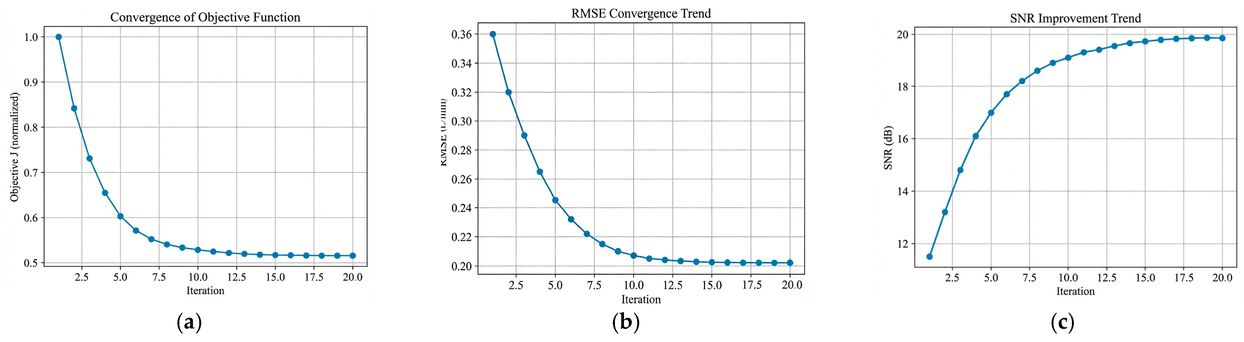
Combined with the continuity of the threshold function (Equation (23)), which eliminates the discontinuity of hard thresholding and the bias of soft thresholding, the signal reconstruction error forms a monotonically non-increasing sequence. The experimental results in

Table 4. Convergence experimental analysis.

Iteration	Objective J (Normalized)	RMSE	SNR (dB)	ΔJ	Convergence Status
1	1	0.36	11.5	-	Not converged
2	0.842	0.32	13.2	−0.158	Not converged
3	0.731	0.29	14.8	−0.111	Not converged
4	0.655	0.265	16.1	−0.076	Not converged
5	0.603	0.245	17.0	−0.052	Not converged
6	0.571	0.232	17.7	−0.032	Not converged
7	0.552	0.222	18.2	−0.019	Approaching
8	0.540	0.215	18.6	−0.012	Approaching
9	0.533	0.210	18.9	−0.007	Approaching
10	0.528	0.207	19.1	−0.005	Approaching
11	0.524	0.205	19.3	−0.004	Converged
12	0.521	0.204	19.4	−0.003	Converged
13	0.519	0.2032	19.55	−0.002	Converged
14	0.5175	0.2027	19.65	−0.0015	Converged
15	0.5165	0.2023	19.72	−0.001	Converged
16	0.5158	0.2021	19.78	−0.0007	Converged
17	0.5153	0.2020	19.82	−0.0005	Converged (plateau)
18	0.5151	0.2020	19.84	−0.0002	Converged (plateau)
19	0.5150	0.2020	19.85	−0.0001	Converged (plateau)
20	0.5150	0.2020	19.85	0	Converged (plateau)

confirm this theoretical prediction: RMSE decreases from 0.36 (iteration 1) to 0.2020 (iteration 17) and remains constant thereafter, with $\left|\Delta J\right|<0.001$ after iteration 14, demonstrating convergence in the engineering sense (i.e., the improvement between successive iterations falls below a prescribed tolerance).

The convergence experimental analysis is shown in Table 4, the convergence of the objective function is shown in Figure 11a, the convergence trend of RMSE is shown in Figure 11b, and the improvement trend of SNR is shown in Figure 11c.

5. Experimental Verification

5.1. Implementation and Comparison of Fuzzy-PID in Proportional Control Valves

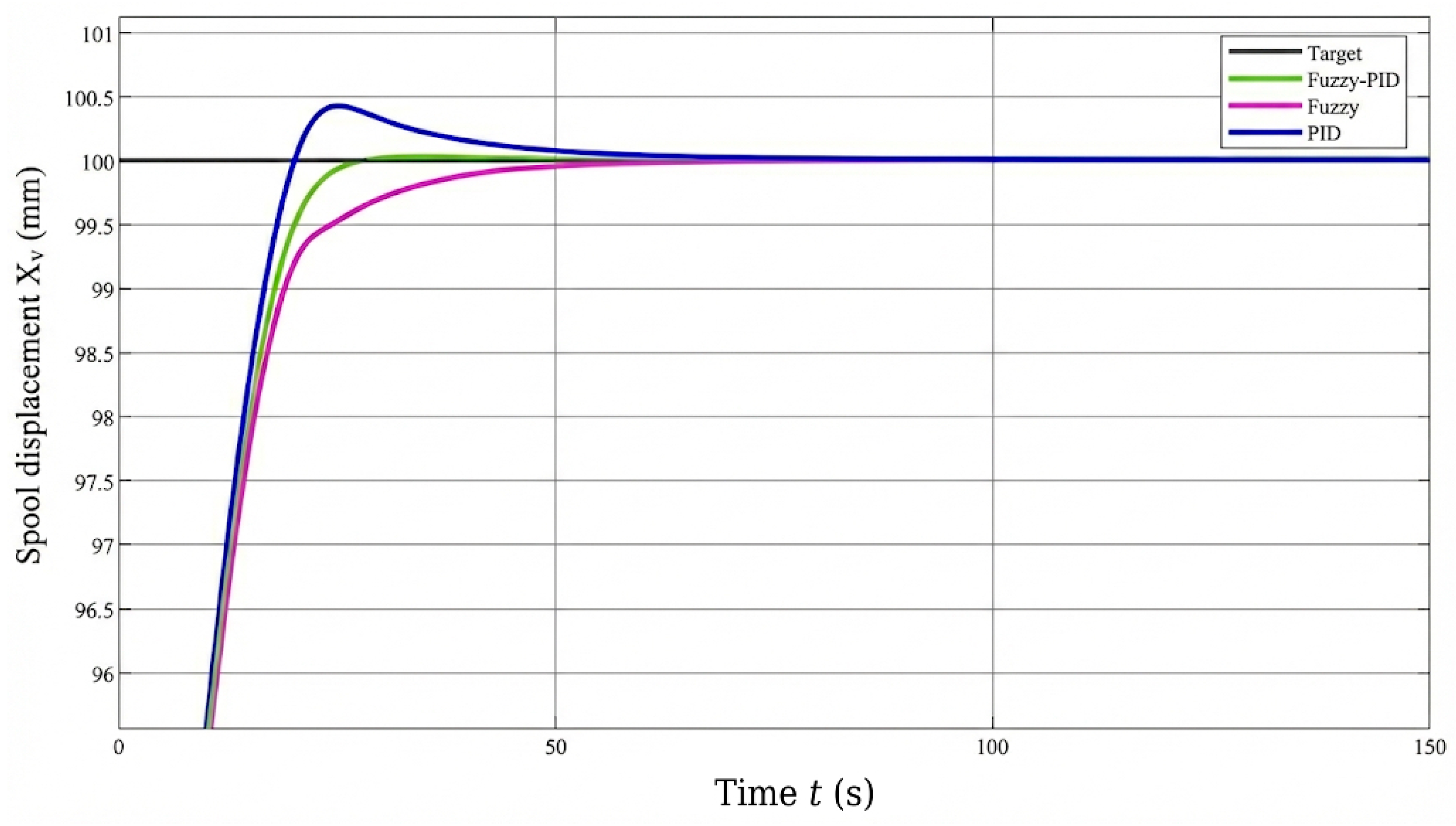
The present study validated the control performance of an electromagnetic pneumatic system. A comparison of the proposed method with traditional PID control and fuzzy control using Matlab R2023b software was conducted to demonstrate the superiority of the proposed method, as illustrated in Figure 12. As depicted in the figure, both fuzzy PID control (green line) and fuzzy control (purple line) achieve the target value (black line) more rapidly than traditional PID control (blue line), indicating that fuzzy PID control possesses a faster response time. In contrast, traditional PID control (blue line) demonstrates significant overshoot before attaining the target value, the target value is exceeded prior to stabilization in both the fuzzy PID control (green line) and fuzzy control (purple line) models. However, the overshoot values are smaller in the former, suggesting that fuzzy PID control is more effective in reducing overshoot. Furthermore, the fuzzy PID control (green line) stabilizes rapidly upon reaching the target value and maintains stability with minimal fluctuations. In contrast, the traditional PID control (blue line) continues to exhibit slight fluctuations after stabilization. The fuzzy PID control (green line) demonstrates superior performance in maintaining stability when confronted with changes in system parameters or external disturbances. This phenomenon can be discerned by examining its capacity to sustain stability subsequent to attaining the target value. The fuzzy PID control (green line) demonstrates a reduced discrepancy between its output value and the target value after attaining the target value, signifying enhanced control precision. Furthermore, the fuzzy PID control (green line) exhibits a seamless transition process devoid of the oscillations evident in the conventional PID control (blue line), suggesting that fuzzy PID control facilitates more refined control performance.

In summary, electromagnetic pneumatic systems exhibit strong nonlinearity, rendering traditional fixed-parameter PID control ineffective for dynamic operating conditions. The integration of fuzzy control with PID control, a combination referred to as “fuzzy PID control,” offers a unique approach by combining the flexibility of fuzzy control with the stability of PID control. A high $K_{\mathrm{p}}$ value enhances the system’s resistance to displacement errors, rendering it suitable for suppressing positioning errors caused by friction. Conversely, a low $K_{\mathrm{p}}$ value prevents flow overshoot in high-pressure zones by adjusting $K_{\mathrm{d}}$ to real-time offset the inertial forces of the cylinder piston, thereby suppressing high-frequency vibrations. This configuration offers several advantages, including enhanced responsiveness, reduced overshoot, improved stability, and enhanced control accuracy. The merits of fuzzy PID control become particularly evident in the context of electromagnetic control systems, where high precision and rapid response are paramount. A comprehensive experimental analysis reveals that the average overshoot of fuzzy PID is 4.2%, in comparison to 6.5% for traditional PID. This represents a 35% reduction, effectively mitigating flow overshoot during valve core startup. In the context of valve core sudden load change tests, resulting in a steady-state error that is lower than that of the traditional PID system. This outcome serves to demonstrate the adaptability of the fuzzy PID system in highly nonlinear scenarios.

5.2. Verification of Flow Estimation Accuracy of Proportional Valves in Noisy Environments

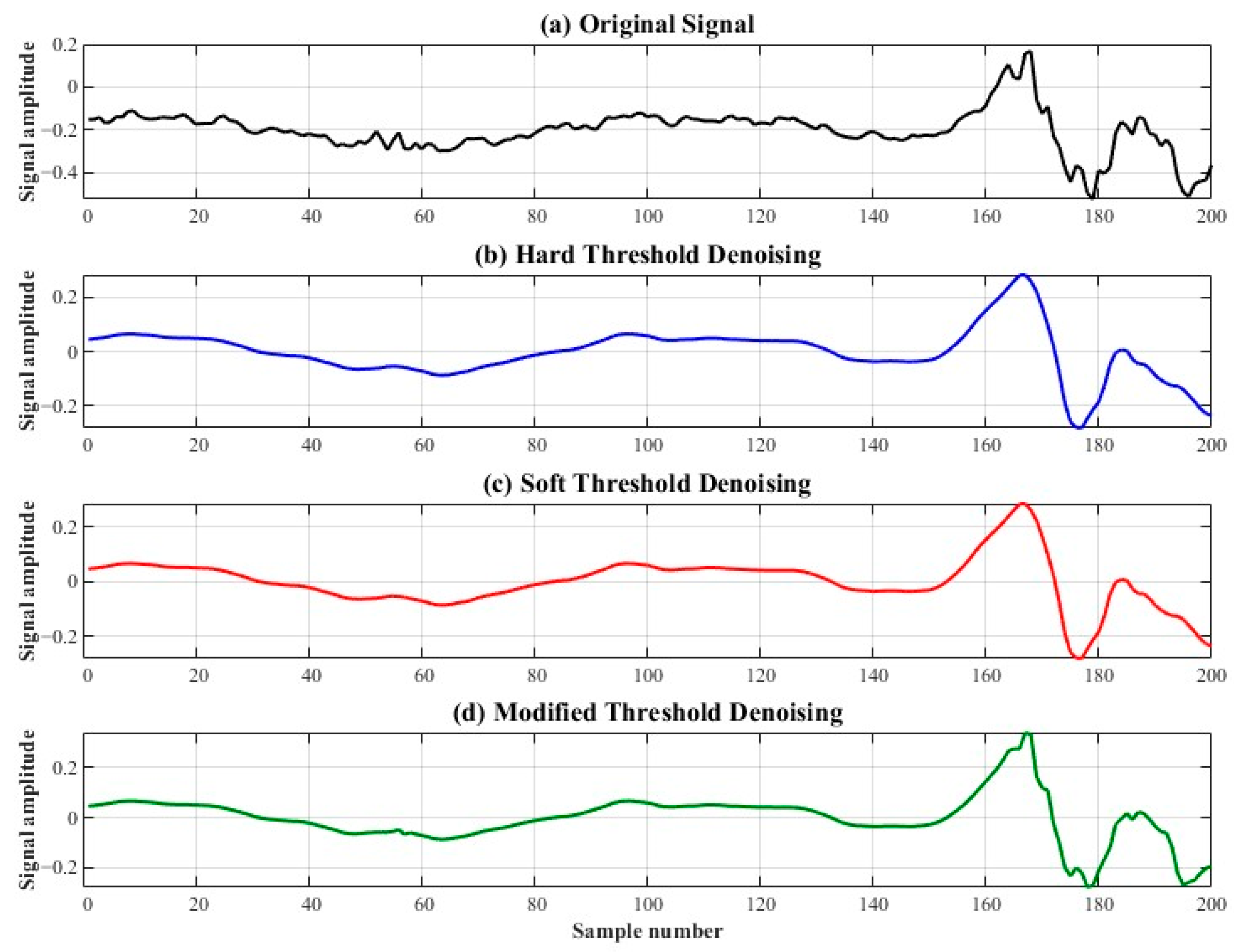
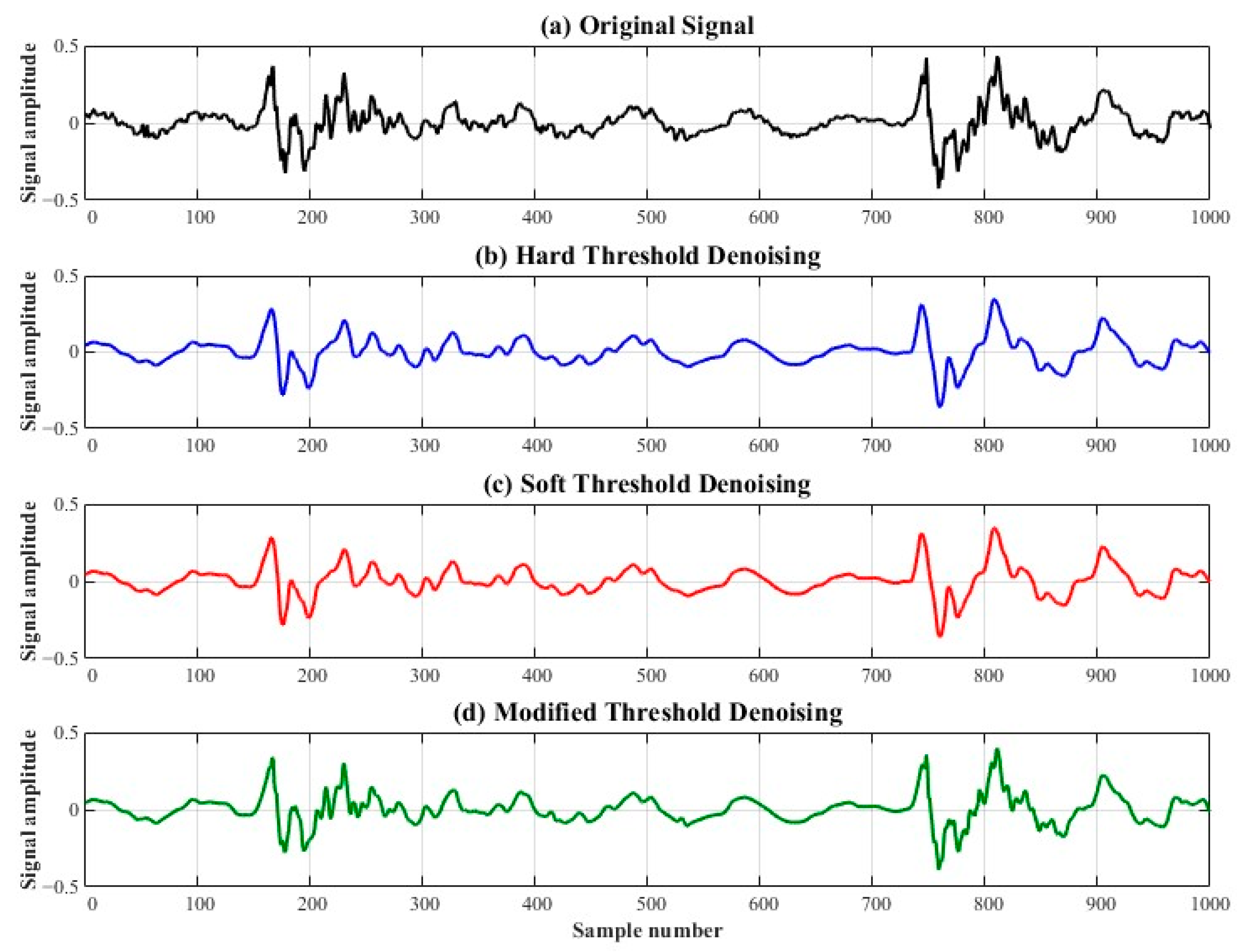
As shown in Figure 13 and Figure 14, The experimental design involved the implementation of conventional hard threshold denoising, soft threshold denoising, and enhanced denoising methodologies, employing 200 and 1000 signal points, respectively. The signal-to-noise ratio (SNR) and root mean square error (RMSE) were utilized as evaluation criteria. A higher signal-to-noise ratio (SNR) and lower root mean square error (RMSE) are indicative of superior denoising performance. The threshold determination method for both hard threshold and soft threshold is the minimum root mean square error (SURE). The threshold type is designated as the global threshold, and the wavelet basis function is the fourth-order Doubchey wavelet.

In order to facilitate a more intuitive and accurate comparison of the data results, the graphs of 1000 data points after noise reduction were compared.

The experimental results suggest that hard thresholding sets coefficients below a certain threshold to zero, while coefficients above the threshold remain unchanged. Consequently, specific components of the signal may become more uniform after the implementation of hard thresholding; However, this process can result in the loss of certain details, thereby inducing discontinuities. In contrast, traditional soft thresholding involves the subtraction of the threshold from all coefficients and the subsequent setting of the result to zero if it is negative. While this method reduces discontinuities compared to hard thresholding, it may cause some parts of the signal to be overly smoothed. The enhanced thresholding method has been shown to enhance the preservation of signal details while concomitantly reducing noise, particularly in complex signals. This approach has been demonstrated to achieve a superior balance between preserving signal details and reducing noise. According to the evaluation criteria, the SNR of the enhanced threshold processing on 200 datasets is 14.4925, and the RMSE is 0.0187544. When processing 1000 datasets, the SNR has been shown to improve from 9.08 dB to 14.98 dB, representing a 64.9% increase, while the RMSE has been shown to decrease from 0.035 to 0.017, representing a 49% reduction. As shown in

Table 5. Evaluation of noise reduction effects of various algorithms.

Database	Noise Reduction Methods	SNR (dB)	RMSE (L/min)
200 × 1	Hard threshold denoising	9.046	0.035108
	Soft threshold denoising	9.046	0.035108
	Noise reduction processing after threshold improvement	14.4925	0.018754
1000 × 1	Hard threshold denoising	9.082	0.034386
	Soft threshold denoising	9.082	0.034386
	Noise reduction processing after threshold improvement	14.9802	0.017437

, A comparison of the improved threshold method with traditional hard threshold and soft threshold methods reveals a substantial enhancement in SNR and a notable reduction in RMSE. This outcome signifies a superior noise reduction performance for the improved threshold method.

To further validate the practical applicability of the proposed method, robustness tests under varying noise and load conditions were conducted. In order to be closer to the actual industrial environment, this paper introduces multiple noise intensity disturbance conditions based on the original uniform noise model to verify the robustness of the proposed method. Three noise levels are specifically set, corresponding to low signal-to-noise ratio, medium signal-to-noise ratio and high signal-to-noise ratio, respectively, and high-frequency electromagnetic noise and low-frequency pressure fluctuation noise are superimposed.

Experimental results show that the improved wavelet threshold method can maintain a high signal-to-noise ratio improvement effect under different noise intensities, verifying the applicability of the method in complex industrial noise environments. As shown in

Table 6. Robustness verification table under different noise and disturbance conditions.

Test Condition	Noise Level (dB)	Disturbance Load (N)	Overshoot (%)	Settling Time (s)	Steady-State Error (mm)	Performance Evaluation
Ideal laboratory condition	0	0	4.2	0.63	0.18	Optimal performance
Low noise	30	50	4.6	0.67	0.21	Stable with minor fluctuation
Moderate noise	50	100	5.3	0.72	0.26	Good robustness
High noise	70	150	6.4	0.81	0.33	Slight oscillation observed
Severe disturbance	85	200	7.8	0.95	0.45	Performance degraded but controllable

.

5.3. Traffic Estimation Implementation

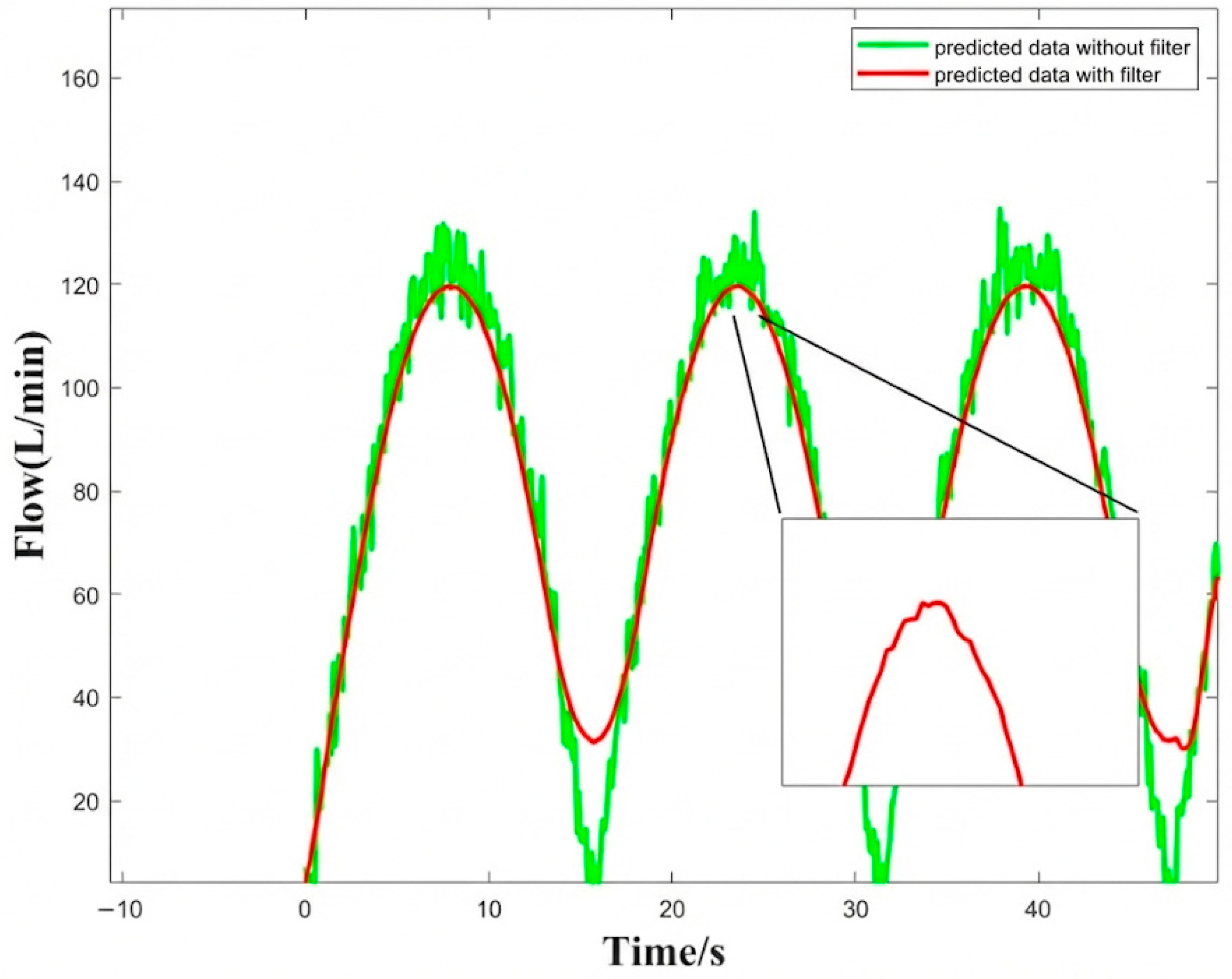
To make a comparison, a sine signal was used to demonstrate the difference between flow estimation based on the improved wavelet denoising method and flow estimation based on the original signal. The results are shown in Figure 15. It can be observed that using filtered training data for model training and filtered test data for prediction yields signals with reduced noise information and smoother overall curves, resulting in a significant reduction in prediction error. In contrast, using the original data for model training and prediction introduces a large amount of noise into the prediction data. These interferences are caused by two factors: (1) the presence of noisy segments in the training data affects the model’s accuracy, and (2) using signals susceptible to noise interference during the testing phase, especially pressure signals, introduces high-frequency noise into the predicted flow signals. During the control process, the presence of high-frequency noise in feedback signals can cause system instability and affect control accuracy. Therefore, improving the wavelet denoising method can enhance the model’s accuracy and mitigate the impact of noise in the perceived signals on the predicted flow signals.

5.4. Comparison of Multi-Method Flow Inference Performance

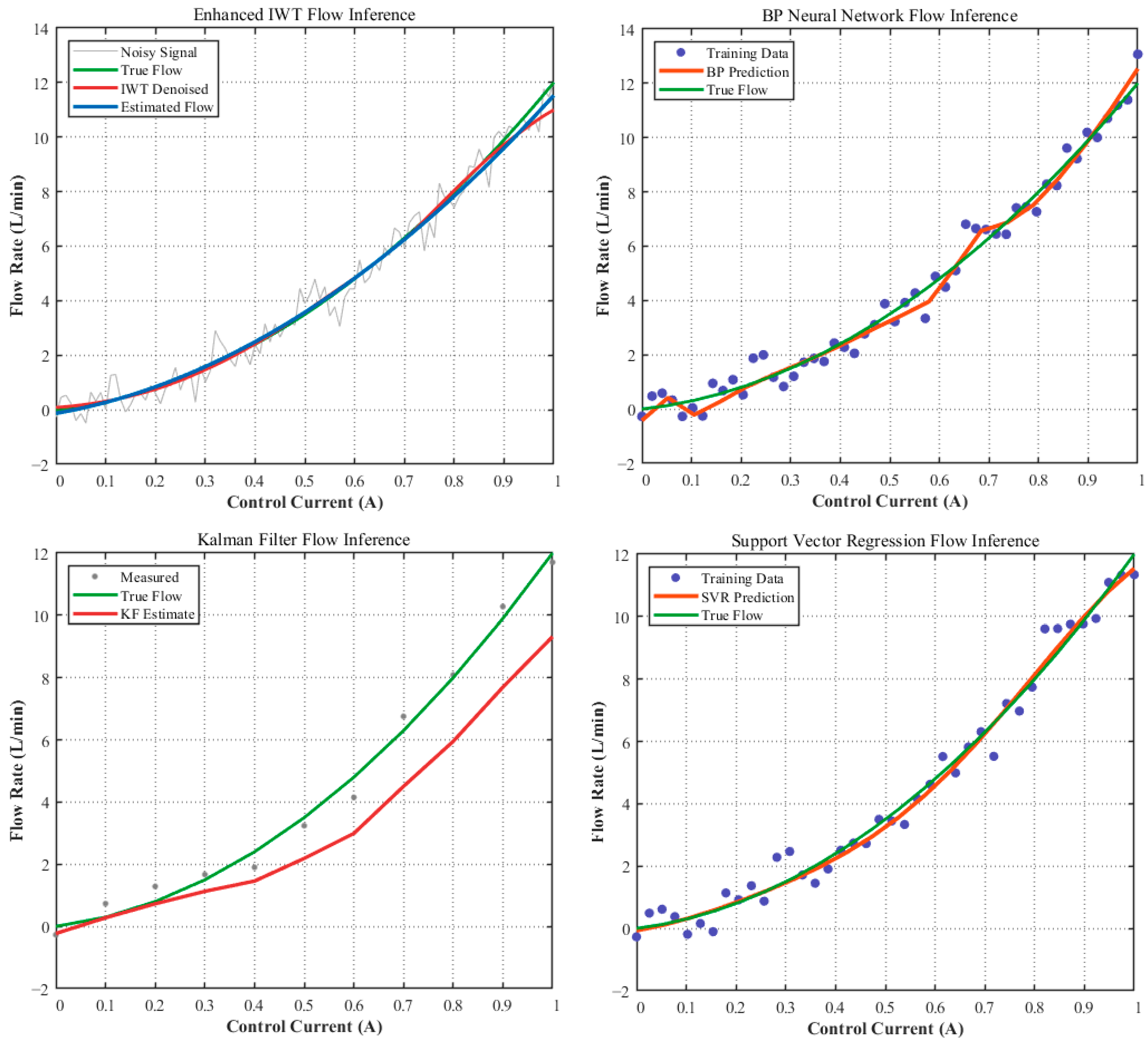
The objective of this section is to validate the superiority of improved wavelet denoising (IWT) in flow estimation. To this end, a comparative experiment is conducted in which IWT is compared with three mainstream methods: BP neural networks, Kalman filtering, and support vector regression (SVR). A strictly controlled comparison framework is adopted to ensure the fairness of the results. All methods utilize the same nonlinear system model, which is based on actual valve characteristic curves. The training set and test set utilize the same noise model, with 0.5 standard deviation of random noise added to simulate the Gaussian noise typically present in sensor measurements, superimposed on the real flow signal. A fixed random seed is employed to ensure noise consistency. The evaluation metrics are uniformly defined as SNR, RMSE, and computation time. To ensure the validity of the findings, all metrics were calculated using the same code to eliminate implementation differences. Furthermore, the current range of the test set was extended beyond that of the training set to rigorously validate the generalization capability of the methods. Furthermore, all experiments were conducted within the same software and hardware environment to eliminate platform dependency. The flow estimation curves of the multi-methods under the same test signals are shown in Figure 16, and the evaluation metrics are presented in

Table 7. Multi-method flow estimation evaluation.

Method	SNR (dB)	RMSE (L/min)	Time (ms)
Improved wavelet denoising (IWT)	22.707	0.413	2.303
BP neural network (BPNN)	18.815	1.063	12.819
Kalman filter (KF)	20.648	0.542	0.028
Support vector regression (SVR)	21.421	0.485	6.457

.

In summary, BP neural networks, as a classic data-driven method based on gradient descent for approximating nonlinear functions, are suitable for the complex nonlinear systems of pneumatic electromagnetic proportional valves. Following the training process, the system demonstrates the capacity to execute computations expeditiously, exhibiting commendable real-time performance. However, these models are heavily reliant on substantial training data, and the training process may exhibit slow convergence, rendering them susceptible to noise in the training set. Kalman filtering is a dynamic estimation method based on state-space models, making it suitable for flow estimation in linear systems and noisy environments. It exhibits low computational complexity but is contingent upon an accurate system model and performs inadequately in highly nonlinear pneumatic systems. Support vector regression is a nonlinear regression method based on the principle of minimization. The method demonstrates robustness to small sample data and exhibits good generalization ability. However, it is characterized by complex parameter tuning, high computational complexity, extended training time, and insufficient robustness in practical applications. The improved wavelet denoising method proposed in this paper employs adaptive threshold denoising to effectively remove noise while preserving the key features of the flow signal, thereby improving signal fidelity. The model is integrated with least-squares regression for flow estimation, a process that enhances estimation accuracy and prevents overfitting, while demonstrating robust noise resistance. Furthermore, wavelet analysis has the capacity to process nonlinear and non-stationary signals, rendering it well-suited for the intricate flow characteristics exhibited by nonlinear pneumatic-electromagnetic proportional valve systems.

The experimental data demonstrate that IWT exhibits significant superiority in key performance metrics. Specifically, its signal-to-noise ratio (SNR = 22.707 dB) is 1.29 dB higher than that of the second-best method, support vector regression (SVR, 21.421 dB). IWT also outperforms the Kalman filter (KF) in denoising accuracy, with its SNR (22.707 dB) being 2.059 dB higher than that of KF (20.648 dB). The root mean square error (RMSE) of the IWT model is 0.413, the lowest among all tested algorithms—approximately 61.2% lower than the RMSE of the BP neural network (BPNN, 1.063) and 14.8% lower than that of SVR (0.485), indicating superior estimation accuracy. Furthermore, IWT achieves excellent computational efficiency (2.303 ms) while maintaining high precision: it is significantly faster than BPNN (12.819 ms) and SVR (6.457 ms), and although it is slightly slower than KF (0.028 ms), it far surpasses KF in denoising accuracy. Enhanced wavelet denoising employs an adaptive threshold function and a hierarchical denoising strategy, thereby effectively mitigating noise while preserving signal nuances. This approach eliminates the need for substantial training data and adapts to nonlinear systems, thereby overcoming the underfitting tendency of BP neural networks in scenarios with limited training data. The proposed approach circumvents the limitations of Kalman filtering under linear assumptions, which are associated with a model mismatch. Additionally, it evades the computational bottlenecks that are prevalent in SVR implementations during large-scale hyperparameter optimization. This solution offers high precision and low latency flow estimation in complex industrial scenarios.

6. Summary

The present paper puts forth a novel electromagnetic pneumatic system control and flow estimation method that integrates fuzzy PID control with improved wavelet transform (IWT), thereby demonstrating significant innovation and engineering value. In terms of control strategy, the collaborative framework of fuzzy PID and IWT effectively addresses the nonlinearity and noise interference issues in electromagnetic pneumatic systems. The dynamic parameter tuning mechanism has been demonstrated to enhance control accuracy and response speed. The experimental results indicate that fuzzy PID control reduces overshoot by 35% compared to traditional methods, while also significantly decreasing steady-state error. This notably enhances the system’s dynamic performance and robustness. With respect to flow estimation, an advanced improved wavelet threshold denoising technique (IWT) is employed, which achieves a balance between noise reduction and signal fidelity through an adaptive threshold function and a hierarchical denoising strategy. The efficacy of the proposed method was validated on a test dataset, which demonstrated that it achieves a more than 65% improvement compared to traditional hard/soft threshold methods. This improvement enables high-precision flow estimation. In engineering applications, the method replaces high-cost sensors through algorithm optimization, thereby reducing equipment complexity and maintenance costs. The device is particularly well-suited for precise control of electromechanical systems in harsh industrial environments, including smart manufacturing, robotics, and high-precision pneumatic actuators. The research findings provide theoretical support and technical pathways for low-cost, high-reliability control solutions in the field of industrial automation, demonstrating broad application potential.

7. Future Prospects

This study enhanced the control accuracy and flow estimation performance of an electromagnetic pneumatic system through the collaborative optimization of fuzzy PID and improved wavelet threshold (IWT). Nevertheless, there remain certain deficiencies and potential areas for enhancement. In this study, the parameters of the adaptive wavelet threshold require manual adjustment. In the future, a genetic algorithm-based automatic parameter tuning framework for wavelet thresholds can be developed to reduce manual intervention. Furthermore, experimental verification was primarily conducted in a simulation environment. In order to enhance the model’s generalization capability, future research should validate the long-term stability and interference resistance of the system in real industrial scenarios with high temperatures and pressures. Conversely, the present study concentrates on single-valve systems. Future research could extend the approach to multi-valve parallel or series systems for cooperative control, investigating the cooperative control strategies under coupled effects and their impact on flow estimation accuracy.

References

1. Xu, B.; Shen, J.; Liu, S.; Su, Q.; Zhang, J. Research and development of electro-hydraulic control valves oriented to industry 4.0: A review. Chin. J. Mech. Eng. 2020, 33, 29. [Google Scholar] [CrossRef] [Scilit]
2. Ahn, K.; Yokota, S. Intelligent switching control of pneumatic actuator using on/off solenoid valves. Mechatronics 2005, 15, 683–702. [Google Scholar] [CrossRef] [Scilit]
3. Topçu, E.E.; Yüksel, İ.; Kamış, Z. Development of electro-pneumatic fast switching valve and investigation of its characteristics. Mechatronics 2006, 16, 365–378. [Google Scholar] [CrossRef] [Scilit]
4. Messina, A.; Giannoccaro, N.I.; Gentile, A. Experimenting and modelling the dynamics of pneumatic actuators controlled by the pulse width modulation (pwm) technique. Mechatronics 2005, 15, 859–881. [Google Scholar] [CrossRef] [Scilit]
5. Sorli, M.; Gastaldi, L.; Codina, E.; de las Heras, S. Dynamic analysis of pneumatic actuators. Simul. Pract. Theory 1999, 7, 589–602. [Google Scholar] [CrossRef] [Scilit]
6. Ali, H.I.; Noor, S.B.; Bashi, S.M.; Marhaban, M.H. A review of pneumatic actuators (modeling and control). Aust. J. Basic Appl. Sci. 2009, 3, 440–454. [Google Scholar]
7. Rao, Z.; Bone, G.M. Nonlinear modeling and control of servo pneumatic actuators. IEEE Trans. Control Syst. Technol. 2008, 16, 562–569. [Google Scholar]
8. Ilchmann, A.; Sawodny, O.; Trenn, S. Pneumatic cylinders: Modelling and feedback force-control. Int. J. Control 2006, 79, 365–378. [Google Scholar] [CrossRef] [Scilit]
9. Lee, H.K.; Choi, G.S.; Choi, G.H. A study on tracking position control of pneumatic actuators. Mechatronics 2002, 12, 813–831. [Google Scholar] [CrossRef] [Scilit]
10. Hodgson, S.; Le, M.Q.; Tavakoli, M.; Pham, M.T. Improved tracking and switching performance of an electro-pneumatic positioning system. Mechatronics 2012, 22, 1–12. [Google Scholar] [CrossRef] [Scilit]
11. Leephakpreeda, T. Fuzzy logic based PWM control and neural controlled-variable estimation of pneumatic artificial muscle actuators. Expert Syst. Appl. 2011, 38, 7837–7850. [Google Scholar] [CrossRef] [Scilit]
12. Santos, M.; Ferreira, J. Novel intelligent real-time position tracking system using FPGA and fuzzy logic. ISA Trans. 2013, 53, 402–414. [Google Scholar] [CrossRef] [Scilit] [PubMed]
13. Świder, J.; Wszołek, G.; Carvalho, W. Programmable controller designed for electro-pneumatic systems. J. Mater. Process. Technol. 2005, 164, 1459–1465. [Google Scholar] [CrossRef] [Scilit]
14. Taghizadeh, M.; Ghaffari, A.; Najafi, F. Improving dynamic performances of pwm-driven servo-pneumatic systems via a novel pneumatic circuit. ISA Trans. 2009, 48, 512–518. [Google Scholar] [CrossRef] [Scilit] [PubMed]
15. Xie, C.; Su, H. Design and analysis of combined valve spool with linear flow coefficient. J. Eng. 2022, 2022, 6006810. [Google Scholar] [CrossRef] [Scilit]
16. Valdés, J.R.; Rodríguez, J.M.; Saumell, J.; Pütz, T. A methodology for the parametric modelling of the flow coefficients and flow rate in hydraulic valves. Energy Convers. Manag. 2014, 88, 598–611. [Google Scholar] [CrossRef] [Scilit]
17. Viall, E.N.; Zhang, Q. Determining the discharge coefficient of a spool valve. In Proceedings of the 2000 American Control Conference, Chicago, IL, USA, 28–30 June 2000; Volume 5, pp. 3600–3604. [Google Scholar]
18. Zhang, J.; Wang, D.; Xu, B.; Su, Q.; Lu, Z.; Wang, W. Flow control of a proportional directional valve without the flow meter. Flow Meas. Instrum. 2019, 67, 131–141. [Google Scholar] [CrossRef] [Scilit]
19. RÅman, R.; Handroos, H.; Eskola, T. Computationally efficient two-regime flow orifice model for real-time simulation. Simul. Model. Pract. Theory 2008, 16, 945–961. [Google Scholar]
20. Ding, R.; Yan, P.; Cheng, M.; Xu, B. A flow inferential measurement of the independent metering multi-way valve based on an improved RBF neural network. Flow Meas. Instrum. 2023, 223, 113750. [Google Scholar] [CrossRef] [Scilit]
21. Sitte, A.; Koch, O.; Liu, J.; Tautenhahn, R.; Weber, J. Multidimensional flow mapping for proportional valves. In Proceedings of the 12th International Fluid Power Conference, Dresden, Germany, 12–14 October 2020; Volume 1, pp. 231–240. [Google Scholar]
22. Cao, Y.; Huang, J.; Xiong, C.H.; Wu, D.; Zhang, M.; Li, Z.; Hasegawa, Y. Adaptive Proxy-Based Robust Control Integrated with Nonlinear Disturbance Observer for Pneumatic Muscle Actuators. IEEE/ASME Trans. Mechatron. 2020, 25, 1756–1764. [Google Scholar] [CrossRef] [Scilit]
23. Cao, J.; Xie, S.Q.; Das, R. MIMO Sliding Mode Controller for Gait Exoskeleton Driven by Pneumatic Muscles. IEEE Trans. Control Syst. Technol. 2018, 26, 274–281. [Google Scholar] [CrossRef] [Scilit]
24. Najjari, B.; Barakati, S.M.; Mohammadi, A.; Futohi, M.J.; Bostanian, M. Position control of an electro-pneumatic system based on PWM technique and FLC. ISA Trans. 2014, 53, 647–657. [Google Scholar] [CrossRef] [Scilit]
25. Phu, N.D.; Hung, N.N.; Ahmadian, A.; Senu, N. A new fuzzy PID control system based on fuzzy PID controller and fuzzy control process. Int. J. Fuzzy Syst. 2020, 22, 2163–2187. [Google Scholar] [CrossRef] [Scilit]
26. Meng, F.; Liu, S.; Liu, K. Design of an optimal fractional order PID for constant tension control system. IEEE Access 2020, 8, 58933–58939. [Google Scholar] [CrossRef] [Scilit]
27. Dong, W.Y.; Ding, H.; Dong, X.S.; Wang, Y.F. An adaptive wavelet threshold denoising both in low and high frequency domains. Acta Electron. Sin. 2015, 43, 2374–2380. [Google Scholar]
28. Gouizi, K.; Reguig, F.B.; Maaoui, C. Discrete wavelet transform analysis and empirical mode decom-position of physiological signals for stress recognition. Int. J. Biomed. Eng. Technol. 2018, 27, 247–270. [Google Scholar] [CrossRef] [Scilit]
29. Tang, J.; Zhou, S.; Pan, C. A denoising algorithm for partial discharge measurement based on the combination of wavelet threshold and total variation theory. IEEE Trans. Instrum. Meas. 2019, 69, 3428–3441. [Google Scholar] [CrossRef] [Scilit]
30. Ma, Z.; Chen, Y.; Zhang, T.; Liao, Z. An enhanced spectral amplitude modulation method for fault diagnosis of rolling bearings. Machines 2024, 12, 779. [Google Scholar] [CrossRef] [Scilit]
31. Chen, P.; Zhao, X. Early fault feature extraction of rolling bearings based on optimized VMD and improved threshold denoising. J. Vib. Shock 2021, 40, 146–153. [Google Scholar]
32. Yang, Z.; Huo, Y. Research on bearing signal denoising based on improved wavelet algorithm. Chin. J. Eng. Mach. 2020, 18, 40–44. [Google Scholar]
Figure 1. Stribeck friction model.
Actuators 15 00141 g001
Figure 2. LuGre friction model.
Actuators 15 00141 g002
Figure 3. Comparison of the Stribeck friction model and the LuGre friction model.
Actuators 15 00141 g003
Figure 4. Valve model subsystem.
Actuators 15 00141 g004
Figure 5. Schematic diagram of the experimental setup.
Actuators 15 00141 g005
Figure 6. Structure diagram of fuzzy PID controller.
Actuators 15 00141 g006
Figure 7. Triangular membership functions for input variables e , e ˙ and output variables K p ,   K i ,   K d .
Actuators 15 00141 g007
Figure 8. Parameter optimization process chart.
Actuators 15 00141 g008
Figure 9. Overshoot variation under parameter perturbations.
Actuators 15 00141 g009
Figure 10. Schematic diagram of the wavelet tree structure.
Actuators 15 00141 g010
Figure 11. (a) Convergence of objective function; (b) RMSE convergence trend; (c) SNR improvement trend.
Actuators 15 00141 g011
Figure 12. Comparison of fuzzy PID and traditional PID control performance.
Actuators 15 00141 g012
Figure 13. Noise reduction effect of 200 data points using wavelet soft and hard thresholds and improved threshold.
Actuators 15 00141 g013
Figure 14. Noise reduction effect of 1000 data points using wavelet soft and hard thresholds and improved thresholds.
Actuators 15 00141 g014
Figure 15. Flow estimation waveforms before and after improved wavelet processing.
Actuators 15 00141 g015
Figure 16. Comparison of multi-method flow inference results.
Actuators 15 00141 g016