Research on Stewart Platform Control Method for Wave Compensation Based on BiLSTM Prediction and ADRC

Abstract

Offshore operational environments are inherently stochastic, with waves, currents, and wind loads exerting a significant influence on vessel attitude and equipment stability. While Stewart platforms enable active motion compensation, conventional control strategies frequently suffer from time delays, actuator lag, and limited disturbance rejection, resulting in inadequate performance under complex sea conditions. To overcome these limitations, this paper presents a wave compensation control strategy for a Stewart platform that integrates deep learning-based prediction with active disturbance rejection control (ADRC). A bidirectional long short-term memory (BiLSTM) network is developed to predict vessel attitude in advance. The predicted attitude is transformed into actuator displacement commands through the inverse kinematics of the Stewart platform. An ADRC-based displacement controller is then designed to achieve fast and robust compensation under wave disturbances. Six-degree-of-freedom (6-DOF) dynamic models of a catamaran and a Stewart platform are established in Simulink and Simscape, and sea states 2, 4, and 6 are simulated using an enhanced Joint North Sea Wave Project (JONSWAP) wave spectrum. The simulation results show that, compared with Proportional–Integral–Derivative (PID) and ADRC methods, the proposed BiLSTM-ADRC strategy reduces the roll root mean squared error (RMSE) by 76.6% and 73.2%, and pitch RMSE by 64.1% and 58.1%, respectively, demonstrating an improved attitude stabilization performance.

1. Introduction

In realistic marine environments, continuous stochastic disturbances from wind, waves and currents induce pronounced vessel attitude motions that can severely compromise the stability and operational safety of on-board precision equipment. To mitigate these effects, shipborne Stewart platforms, interposed between the ship’s structure and the payload, have emerged as highly promising wave compensation solutions [1,2,3]. They are increasingly deployed in applications such as precision instrumentation and offshore access gangways [4].

In a typical arrangement, the lower platform is rigidly attached to the hull and follows the ship motion, whilst the upper platform maintains a constant pose in an inertial frame through the coordinated adjustment of the six actuated leg lengths, thereby markedly enhancing payload self-stabilization and the rejection of environmental disturbances [5]. However, the strong coupling and pronounced nonlinear characteristics intrinsic to Stewart platforms impose stringent demands on the real-time performance, accuracy and robustness of the associated control systems [6,7].

Given the wide application prospects of Stewart platforms, substantial effort has recently been directed towards the control design of ship-mounted systems [8,9,10]. He et al. introduced a model-free nonsingular fast terminal sliding-mode controller to track the position and attitude of Stewart platforms [11]. Safeen et al. modified the integral sliding-mode algorithm and proposed an adaptive super-twisting smooth integral sliding-mode controller [12], which enhances disturbance rejection through adaptive mechanisms but entails a complex structure and considerable real-time computational load. Cai et al. developed a velocity feed-forward compensator within a sliding-mode framework to improve dynamic performance [13], achieving a better disturbance compensation while leaving scope for improved real-time velocity responsiveness. Wen et al. integrated time delay estimation and Kalman filter-based adaptive estimation into a nonsingular terminal sliding-mode controller to account for gravitational effects, markedly improving robust control accuracy [14]. Chen et al. proposed a three-loop active disturbance rejection control architecture for electrically driven, ship-mounted Stewart platforms comprising an internal-model controller in the current loop for rapid torque adaptation, a sliding-mode controller in the velocity loop for speed stabilization, and ADRC in the position loop to estimate and compensate total position disturbances. Relative to conventional PI control, this approach delivered significant improvements in both compensation accuracy and the smoothness of the compensated motion [15]. Liu et al. combined the beetle antennae search algorithm with radial basis function neural networks to obtain an improved adaptive control strategy [16], although its generalization capability requires further enhancement. Model Predictive Control (MPC) has been widely applied to Stewart platforms due to its ability to explicitly handle multivariable coupling and system constraints. Qiang et al. proposed an MPC strategy for shipborne stabilization platforms to effectively address load disturbances, improving platform stability and robustness under external excitations [17]. Wang et al. implemented an MPC framework that computes additional control inputs online within the prediction horizon to solve the optimal control problem for multi-degree-of-freedom platforms, achieving more precise trajectory tracking while satisfying constraints [18]. More recently, adaptive MPC has been applied to high-precision pointing control tasks, efficiently handling input nonlinearities, parameter uncertainties, and periodic disturbances [19]. In parallel, deep learning techniques have been increasingly adopted in control algorithm design, giving rise to a variety of advanced control methods. These learning-based approaches leverage the strong nonlinear approximation and sequence modeling capabilities of deep neural networks to replace or enhance modules in traditional control, including system modeling, strategy optimization, and state estimation [20]. Li et al. proposed a neural network-based backpropagation (BP) PID control algorithm, where the PID parameters are adaptively adjusted by the BP network to quickly achieve optimal performance [21]. Yin et al. introduced a relaxation deep learning (RDL) framework by incorporating relaxation operators into deep neural networks, which enables unified real-time economic dispatch and control across multiple time scales [22]. To improve disturbance rejection and robustness, Wang et al. developed a control method based on adversarial deep reinforcement learning to address deep tracking problems for underactuated autonomous underwater vehicles with inherent coupled dynamics and external disturbances [23]. Deep neural networks have also been applied to nonlinear system identification; for example, in greenhouse modeling and control, Elman networks have been trained to simulate system dynamics directly, while multilayer perceptrons (MLPs) have been used for controller design [24].

Despite these advances, the reliable deployment of Stewart platform control in complex marine environments remains constrained by two principal technical challenges. First, disturbance rejection is hampered by the platform’s strongly nonlinear, time-varying environmental loads from waves, wind and currents [25], which collectively undermine closed-loop stability and robustness under complex sea states [26,27,28]. Second, the control loop exhibits pronounced delay-induced hysteresis: unavoidable latencies accrue across attitude sensing, computation, and actuator execution, and, under severe sea states and high-frequency excitations, these time delays introduce phase lags that cause compensation to trail actual ship motion, thereby degrading attitude stabilization and control accuracy [29].

To address these challenges, a range of advanced strategies have been investigated. Among them, ADRC has attracted considerable interest owing to its strong disturbance rejection capability [30,31]. Zhang et al. [32] proposed a dual-loop ADRC architecture that effectively tackled the nonlinearity, strong coupling and disturbance sensitivity inherent in quadrotor systems. Xu et al. [33] employed a cascaded ADRC scheme for quadrotor path tracking, improving performance in the presence of external disturbances. Qu et al. [34] applied the ADRC extended-state observer (ESO) to electric drives to estimate and suppress endogenous disturbances. Bilal et al. [35] designed a fifth-order ESO-based ADRC controller that achieved the accurate trajectory tracking of a rotary flexible-joint manipulator whilst attenuating lumped disturbances.

To mitigate latency-induced errors, a promising strategy is to forecast the ship attitude ahead of time and apply pre-emptive feed-forward compensation. By providing the controller with a priori estimates of future motion, compensation commands can be issued earlier, substantially reducing the tracking errors attributable to delays. Deep learning offers a powerful toolkit for nonlinear time series modeling; in particular, long short-term memory (LSTM) networks have demonstrated a strong performance in complex ship attitude prediction tasks [36]. BiLSTM architectures can further enhance accuracy and stability by exploiting bidirectional temporal dependencies within the input window [37]. More recently, attention mechanisms have been incorporated to strengthen feature extraction in LSTM-based predictors. For example, Wang et al. [38] combined LSTM with multi-head attention, enabling the model to focus dynamically on salient time steps, thereby improving attitude prediction accuracy and robustness.

Building on these considerations, this study presents an integrated wave motion compensation framework that couples deep learning-based prediction with cascaded ADRC. To accommodate the pronounced randomness, non-stationarity and time-varying characteristics of offshore ship attitude signals, we develop a BiLSTM time series predictor. Structured samples are formed via a sliding-window scheme to forecast near-future attitude variations, providing a priori information to the compensation module. At the control layer, the predictions are embedded in the Stewart platform’s inverse kinematics to issue feed-forward displacement commands to the six actuators, whilst ADRC-based feedback controllers, augmented with a velocity-proportional compensation term, enhance dynamic regulation and disturbance rejection. For validation, we construct a 6-DOF catamaran model and generate representative sea conditions using an improved JONSWAP wave spectrum model, covering sea states 2, 4 and 6. Performance is assessed using multiple control metrics, collectively demonstrating the effectiveness and engineering viability of the proposed method under complex sea states.

The main contributions of this work are as follows:

(1)

An anti-delay ship attitude motion prediction strategy is proposed, in which a BiLSTM neural network forecasts future ship attitudes based on historical data. The predicted results are used to generate feed-forward reference commands for Stewart platform compensation, thereby mitigating the adverse effects of system time delays on compensation accuracy through the advanced acquisition of future attitude information.

(2)

A cascaded control architecture combining position ADRC and proportional velocity control is designed to achieve the hierarchical regulation of the six actuators of the Stewart platform. The strong disturbance rejection capability of ADRC enables the real-time tracking and suppression of external disturbances, while proportional velocity control enhances the system damping, preventing overshoot and oscillations induced by environmental perturbations.

(3)

A 6-DOF dynamic model of a catamaran is developed, and a directionally spread improved JONSWAP wave spectrum is employed to simulate typical sea states of levels 2, 4, and 6, enabling high-fidelity modeling and a simulation-based validation of real marine environmental disturbances.

The remainder of this paper is organized as follows. Section 2 formulates the ship dynamics, the wave spectrum model, and a Simscape-based model of the Stewart platform. Section 3 develops a BiLSTM-based ship attitude predictor and integrates it within a cascaded position-ADRC and proportional velocity control framework to yield an integrated Stewart platform wave motion compensation scheme. Section 4 details simulation scenarios across representative sea states and reports results evaluating the disturbance rejection performance and real-time capability. Section 5 concludes and outlines directions for future work.

2. Mathematical Modeling and System Description

This chapter addresses the critical challenges associated with the significant time delay effects and limited disturbance rejection in wave motion compensation. It presents comprehensive modeling studies of the ship’s 6-DOF dynamics, the JONSWAP wave model, and the Stewart platform. A wave frequency spectrum and directional model are developed to simulate wave environment inputs for the experiments. Furthermore, by integrating the kinematics and dynamics of the Stewart platform, we derive the mathematical relationships between the platform’s pose and actuator motions.

2.1. Catamaran USV Model

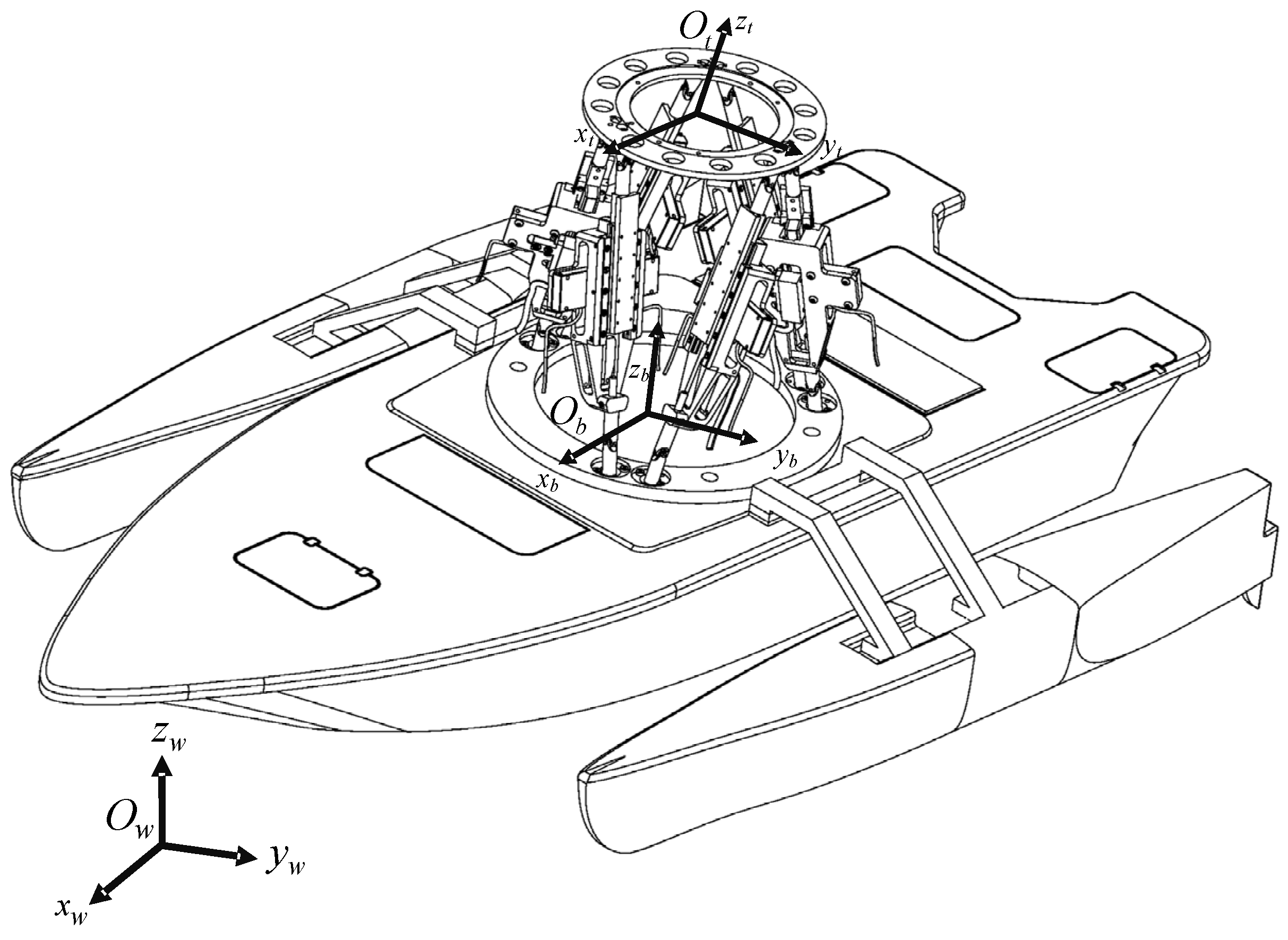
The present study focuses on the Otter catamaran, a classic simulation model within the Marine Systems Simulation (MSS) toolbox in MATLAB R2023a. The Otter catamaran serves as a standardized reference for dynamics research and the simulation validation of nearshore vessels. It is widely utilized in academic research and engineering validation in fields such as ship motion control, hydrodynamic performance analysis, and navigational attitude simulation. The propulsion and control system of the catamaran consists of two propellers positioned on either side of the vessel, enabling yaw control through differential thrust between the left and right propellers. Figure 1 illustrates the catamaran under investigation, with $O_w-x_w{y}_w{z}_w$ representing the world coordinate system, which remains fixed on the Earth and serves as an inertial reference frame. O_b − x_by_bz_b denotes the lower platform coordinate frame, rigidly attached to the ship deck, with its origin O_b located at the center of the coordinate system. O_t – x_ty_tz_t denotes the upper platform coordinate frame, rigidly connected to the upper platform, with its origin $O_t$ located at its center.

In pursuit of capturing the dominant dynamic features while preserving model tractability, a set of simplifying assumptions is incorporated into the 6-DOF modeling of the vessel. The hull is treated as a rigid body, with elastic deformations and propeller–hull coupling effects omitted from the analysis. Additionally, aerodynamic resistance and negligible structural vibrations are excluded from the model formulation.

The Newton–Euler method [39] is employed to derive the 6-DOF kinematic and dynamic model of the vessel.

To describe the position and attitude variations in the catamaran, the following kinematic equations are formulated.

$$\dot{\mathsf{\eta }}=\mathit{J}(\mathsf{\eta })\nu$$

(1)

where $\mathsf{\eta }={[x,y,z,\phi ,\theta ,\psi ]}^T$ denotes the vessel’s position and attitude states in the inertial coordinate frame, while $\mathit{v}={\left[u,v,w,p,q,r\right]}^T$ represents the vessel’s velocity states expressed in the body-fixed coordinate frame. The matrix $\mathit{J}(\mathsf{\eta })$ is the corresponding transformation matrix, defined explicitly as follows.

$$\mathit{J}(\mathsf{\eta })=\left[\begin{array}{cc}\mathit{R}(\mathit{f},\mathsf{\theta },\mathsf{\psi })& {\mathbf{0}}_{3\times 3}\\ 0_{3\times 3}& \mathit{T}(\mathsf{f},\mathsf{\theta })\end{array}\right]$$

(2)

where $\mathit{R}(\mathsf{\phi },\mathsf{\theta },\mathsf{\psi })$ is the rotation matrix constructed from Euler angles $(\phi ,\theta ,\psi )$, describing the transformation between the body-fixed and inertial coordinate frames, while $\mathit{T}(\mathsf{\phi },\mathsf{\theta })$ is the transformation matrix relating attitude angles to angular velocities.

Based on these kinematic relationships, the dynamic equations of the catamaran can be expressed as follows.

$$\mathit{M}\dot{\nu }+\mathit{C}({\nu }_{\mathrm{r}}){\nu }_{\mathrm{r}}+\mathit{G}({\nu }_{\mathrm{r}})\eta =\mathit{D}(v_{\mathrm{r}})v_{\mathrm{r}}+{\tau }_{\mathrm{prop}}+{\tau }_{\mathrm{crossflow}}+\mathit{M}{\dot{\nu }}_{\mathrm{c}}$$

(3)

where $\mathit{M}$ denotes the mass matrix (including both rigid-body and added-mass contributions), $\mathit{C}({\nu }_{\mathrm{r}})$ represents the Coriolis and centripetal matrix, $\mathit{D}({\nu }_{\mathrm{r}})$ denotes the damping matrix, $\mathit{G}({\nu }_{\mathrm{r}})$ represents the hydrostatic restoring matrix, ${\tau }_{\mathrm{prop}}$ denotes the control forces and moments generated by the propellers, ${\tau }_{\mathrm{crossflow}}$ represents the cross-flow drag forces and moments, ${\nu }_{\mathrm{r}}$ denotes the vessel velocity relative to the waves; and $v_{\mathrm{c}}$ denotes the wave-induced velocity.

The total mass matrix is decomposed into rigid-body and added-mass parts. The rigid-body mass matrix is given by

$$\mathit{M}={\mathit{M}}_{\mathrm{RB}}+{\mathit{M}}_{\mathrm{A}}$$

(4)

The rigid-body mass matrix can be expressed as follows:

$${\mathit{M}}_{\mathit{R}\mathit{B}}=\left[\begin{array}{cc}m{\mathit{I}}_{3\times 3}& -m\mathit{S}(r_{\mathrm{g}})\\ m\mathit{S}(r_{\mathrm{g}})& {\mathit{I}}_{\mathit{g}}\end{array}\right]$$

(5)

where $m$ denotes the total mass of the vessel, $S(r_g)$ is the skew-symmetric matrix associated with the position vector from the center of gravity to the coordinate origin, $I_g$ represents the inertia tensor about the center of gravity, and $r_g$ denotes the position of the center of gravity. The added-mass matrix, ${\mathit{M}}_{\mathrm{A}}$, is a diagonal matrix accounting for hydrodynamic added-mass effects, and its specific form is given by ${\mathit{M}}_{\mathrm{A}}=\left[\begin{array}{l}{\mathit{M}}_{{\mathrm{A}}_{11}}{\mathit{M}}_{{\mathrm{A}}_{12}}\\ {\mathit{M}}_{{\mathrm{A}}_{21}}{\mathit{M}}_{{\mathrm{A}}_{22}}\end{array}\right]$.

The Coriolis–centripetal matrix includes both rigid-body and added-mass components; it can be written as

$$\mathit{C}({\mathit{v}}_{\mathrm{r}})=\left[\begin{array}{cc}m\mathit{S}({\nu }_2)& 0_{3\times 3}\\ 0_{3\times 3}& -\mathit{S}(I_{\mathrm{g}}{\nu }_2)\end{array}\right]+\left[\begin{array}{cc}{0}_{3\times 3}& -S({\mathit{M}}_{{\mathrm{A}}_{12}}{\nu }_{c+}{\mathit{M}}_{{\mathrm{A}}_{12}}{\omega }_c)\\ -S({\mathit{M}}_{{\mathrm{A}}_{11}}{\nu }_{c+}{\mathit{M}}_{{\mathrm{A}}_{12}}{\omega }_c)& -S({\mathit{M}}_{{\mathrm{A}}_{21}}{\nu }_{c+}{\mathit{M}}_{{\mathrm{A}}_{22}}{\omega }_c)\end{array}\right]$$

(6)

where $v_2$ denotes the angular velocity components of the vessel, $v_{\mathrm{r}}$ represents the linear velocity components of the ocean current, and ${\omega }_{\mathrm{r}}$ denotes the angular velocity components of the current.

The hydrostatic restoring matrix is defined as follows.

$$\mathit{G}({\nu }_{\mathrm{r}})=diag(0,0,2\rho g{A}_{\mathrm{w}\_\mathrm{pont}},\rho g\nabla G_{\mathrm{MT}},\rho g\nabla G_{\mathrm{ML}},0)$$

(7)

where $\rho$ denotes the density of seawater, $g$ is the gravitational acceleration, $A_{\mathrm{w}\_\mathrm{pont}}$ represents the underwater projected area of each pontoon, $▽$ denotes the drainage volume, $G_{\mathrm{MT}}$ represents the transverse metacentric lever arm, and $G_{\mathrm{ML}}$ represents the longitudinal metacentric lever arm.

The damping matrix, $\mathit{D}({\nu }_{\mathrm{r}})$, accounts for both linear and nonlinear damping effects and is defined as follows.

$$\mathit{D}({\nu }_{\mathrm{r}})={\mathit{D}}_{\mathrm{lin}}+{\mathit{D}}_{\mathrm{quad}}$$

(8)

where ${\mathit{D}}_{\mathrm{lin}}$ denotes the linear damping, while ${\mathit{D}}_{\mathrm{quad}}$ represents the quadratic nonlinear damping, which is proportional to the square of the velocity.

The forces and moments generated by the propellers are defined as follows:

$${\tau }_{\mathrm{prop}}={\mathit{B}}_{\mathrm{prop}}\left[\begin{array}{c}{k}_{\mathrm{T}}{n}_1\left|n_1\right|\\ k_{\mathrm{T}}{n}_2\left|n_2\right|\end{array}\right]$$

(9)

where the rotational speeds of the two propellers are denoted by $n_1$ and $n_2$, respectively. $k_{\mathrm{T}}$ is the thrust coefficient, and $B_{\mathrm{prop}}$ denotes the propeller input matrix.

The cross-flow drag forces and moments, denoted ${\tau }_{\mathrm{crossflow}}$, are defined as

$${\tau }_{\mathrm{crossflow}}=\left[\begin{array}{c}0\\ -{\int }_{-L/2}^{L/2}{\displaystyle \frac{1}{2}}\rho T{C}_{\mathrm{D}}\left|V_r+xr\right|(V_r+xr)dx\\ -{\int }_{-L/2}^{L/2}{\displaystyle \frac{1}{2}}\rho T{C}_{\mathrm{D}}\left|W_r+xq\right|(W_r+xq)dx\\ 0\\ -{\int }_{-L/2}^{L/2}{\displaystyle \frac{1}{2}}\rho T{C}_{\mathrm{D}}x\left|W_r+xq\right|(W_r+xq)dx\\ -{\int }_{-L/2}^{L/2}{\displaystyle \frac{1}{2}}\rho T{C}_{\mathrm{D}}x\left|V_r+xr\right|(V_r+xr)dx\end{array}\right]$$

(10)

where $T$ denotes the draft depth, $C_{\mathrm{D}}$ is the two-dimensional cross-flow drag coefficient, $L$ represents the length of vessel, $B$ denotes the vessel beam, $x$ is the longitudinal position relative to the vessel’s center of gravity, $V_{\mathrm{r}}$ and $W_{\mathrm{r}}$ denote the lateral and vertical relative velocities, respectively, $r$ represents the yaw rate, and $q$ represents the pitch rate.

2.2. Wave Spectrum Model

In this study, we model the sea state with the JONSWAP spectrum, including a peak enhancement factor to capture strongly peaked wind and sea conditions. The resulting spectrum provides the wave excitation forces used in the vessel dynamics; the formulation is shown in Equation (11).

$$S(\omega )=\alpha g^2{\omega }^{-5}\exp \left(-{\displaystyle \frac{5}{4}}{\left({\displaystyle \frac{{\omega }_0}{\omega }}\right)}^4\right){\gamma }^{\exp \left(-{\displaystyle \frac{{(\omega -{\omega }_0)}^2}{2{\sigma }^2{\omega }_0^2}}\right)}$$

(11)

where $\alpha$ denotes the energy scale parameter, $g$ is the gravitational acceleration, $\omega$ represents the angular frequency, ${\omega }_0$ denotes the peak frequency, $\gamma$ is the peak shape parameter, and $\sigma$ denotes the spectral width parameter. The wave energy spectrum function, $S(\omega )$, characterizes the distribution of wave energy per unit angular frequency, reflecting the energy content of different frequency components, and serves as a key function for describing the stochastic properties of ocean waves. Based on the original JONSWAP spectrum, a normalization coefficient, $C$, is introduced to ensure that the total wave energy remains constant under varying peak shape parameters. Its definition is given as follows.

$$C=1-0.287\ln (\gamma )$$

(12)

Taken together, the full JONSWAP spectrum is given by

$$S{(\omega )}_{\mathrm{JONSWAP}}=CS(\omega )$$

(13)

2.3. Stewart Platform Model

The position vectors and rotation angle vectors of the lower and upper platforms relative to the world coordinate frame are denoted by ${\mathit{T}}_{\mathrm{t}}^{\mathrm{w}}=(x_{\mathrm{t}}^{\mathrm{w}},y_{\mathrm{t}}^{\mathrm{w}},z_{\mathrm{t}}^{\mathrm{w}},{\alpha }_{\mathrm{t}}^{\mathrm{w}},{\beta }_{\mathrm{t}}^{\mathrm{w}},{\gamma }_{\mathrm{t}}^{\mathrm{w}})$ and ${\mathit{T}}_{\mathrm{b}}^{\mathrm{w}}=(x_{\mathrm{b}}^{\mathrm{w}},y_{\mathrm{b}}^{\mathrm{w}},z_{\mathrm{b}}^{\mathrm{w}},{\alpha }_{\mathrm{b}}^{\mathrm{w}},{\beta }_{\mathrm{b}}^{\mathrm{w}},{\gamma }_{\mathrm{b}}^{\mathrm{w}})$, respectively. The inverse kinematics method is employed to determine the lengths of the six actuators, with the actuator position vector ${\mathit{l}}_{\mathrm{i}}^{\mathrm{b}}$ expressed as in [40].

$${\mathit{l}}_{\mathrm{i}}^{\mathrm{b}}={\mathit{c}}_{\mathrm{t}}^{\mathrm{b}}+{\mathit{R}}_{\mathrm{t}}^{\mathrm{b}}{\mathit{a}}_{\mathrm{i}}^{\mathrm{t}}-{\mathit{b}}_{\mathrm{i}}^{\mathrm{b}},i=1,2,\dots ,6$$

(14)

where ${\mathit{c}}_{\mathrm{t}}^{\mathrm{b}}$ denotes the position vector of the origin of the upper platform coordinate frame relative to that of the lower platform, and ${\mathit{R}}_{\mathrm{t}}^{\mathrm{b}}$ represents the rotation matrix of the upper platform frame with respect to the lower platform frame. ${\mathit{a}}_{\mathrm{i}}^{\mathrm{t}}$ denotes the position vector of the i-th actuator connection point on the upper platform expressed in the upper platform frame, and ${\mathit{b}}_{\mathrm{i}}^{\mathrm{b}}$ denotes the corresponding position vector on the lower platform. The actuator length is obtained as the norm of the actuator position vector and is expressed as follows:

$$l_{\mathrm{i}}=‖{\mathit{l}}_{\mathrm{i}}^{\mathrm{b}}‖,i=1,2,\dots ,6$$

(15)

By applying the Kane method [41] and combining it with generalized coordinate theory, the complete form of the joint space dynamic equations of the ship-mounted Stewart platform can be derived as follows:

$${\mathit{M}}_{\mathrm{l}}\ddot{l}+{\mathit{C}}_{\mathrm{l}}\dot{l}-{\mathit{G}}_{\mathrm{l}}+\mathit{M}{\ddot{T}}_{\mathrm{t}}^{\mathrm{w}}+\mathit{C}({\nu }_{\mathrm{r}}){\dot{T}}_{\mathrm{t}}^{\mathrm{w}}=f_{\mathrm{a}}$$

(16)

where ${\mathit{M}}_{\mathrm{l}}$, ${\mathit{C}}_{\mathrm{l}}$, and ${\mathit{G}}_{\mathrm{l}}$ denote the inertia matrix, the Coriolis and centripetal matrix, and the gravity matrix, respectively. $\dot{l}$ and $\ddot{l}$ represent the actuator velocities and accelerations, respectively. ${\mathit{f}}_{\mathrm{a}}={(f_{\mathrm{a}1},\dots ,f_{\mathrm{a}6})}^T$ denotes the primary actuation forces generated by the actuators, while $\mathit{M}{\ddot{T}}_{\mathrm{t}}^{\mathrm{w}}$ and $\mathit{C}({\mathsf{\nu }}_{\mathrm{r}}){\dot{T}}_{\mathrm{t}}^{\mathrm{w}}$ represent the inertial forces induced by ship motions.

3. The Proposed Method

3.1. Algorithm Architecture

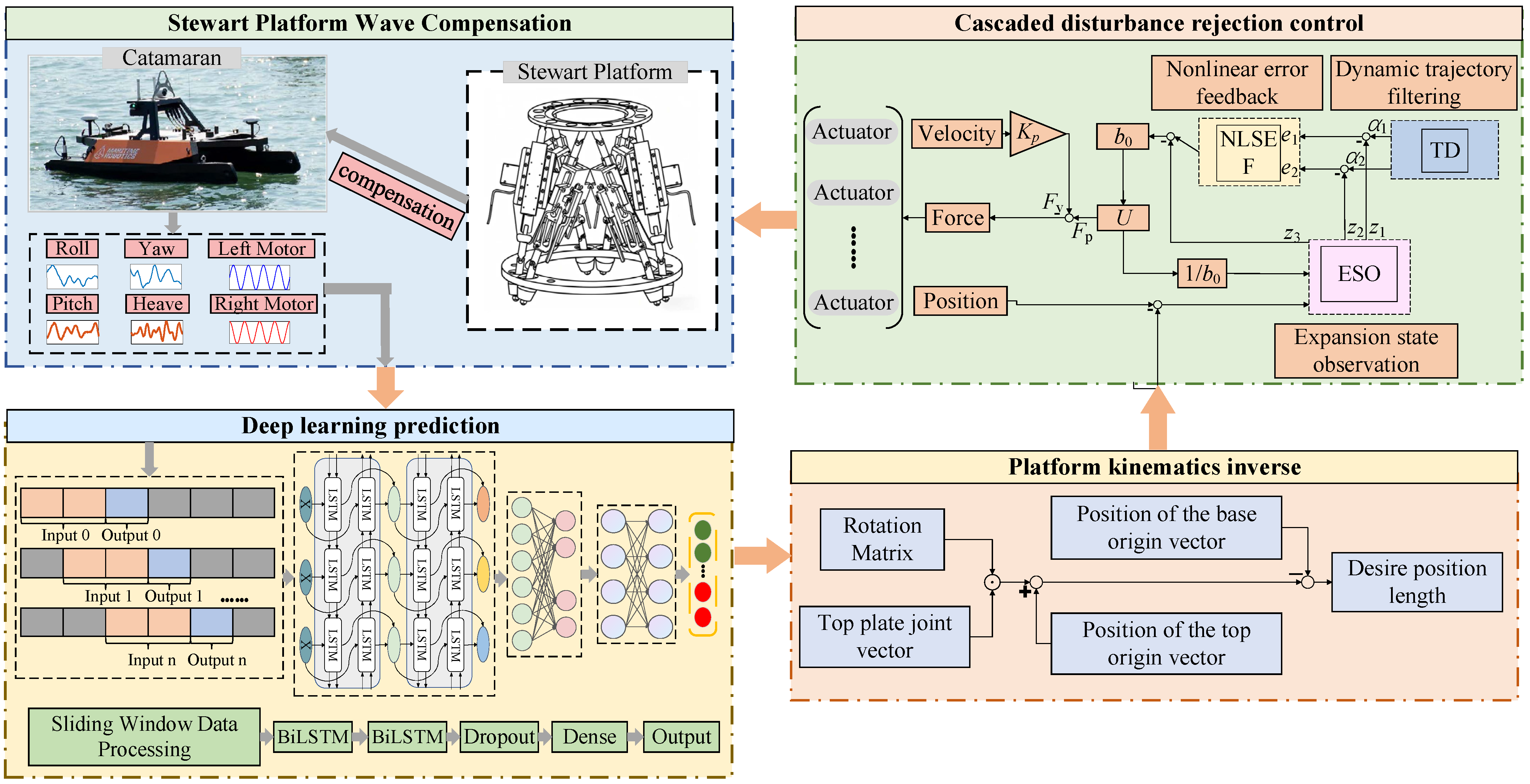
To achieve efficient compensation control for the complex motions of ships, this paper proposes an integrated control framework that combines deep learning-based attitude prediction with a cascaded ADRC strategy. Specifically, the system first collects historical motion data (including roll, pitch, and yaw angles) and control input data of the ship. The raw data are preprocessed using a sliding-window approach and then partitioned into training, validation, and test sets to facilitate the training of the deep learning-based attitude prediction model. Furthermore, the trained deep learning attitude prediction module is deployed online to perform multi-step predictions of the ship’s attitude at future time instants, based on both historical data and the ship’s current control input data. Leveraging the predicted attitude responses, the inverse kinematics model of the Stewart platform is employed to calculate the target lengths of the six actuators, which are then fed as reference inputs to the position controller. The ADRC position controller generates its control output through three core processes: error feedback, state observation, and nonlinear disturbance compensation. Meanwhile, a proportional velocity control scheme produces an auxiliary control signal. The final control command is formulated by fusing the outputs of the ADRC position controller and the proportional velocity controller, which is subsequently applied to the six actuators of the Stewart platform to realize real-time motion compensation. The integrated control framework proposed in this paper is illustrated in Figure 2.

3.2. Deep Learning-Based Attitude Prediction Algorithm

3.2.1. Model Architecture

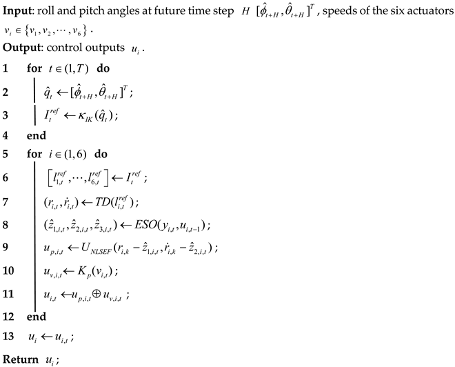
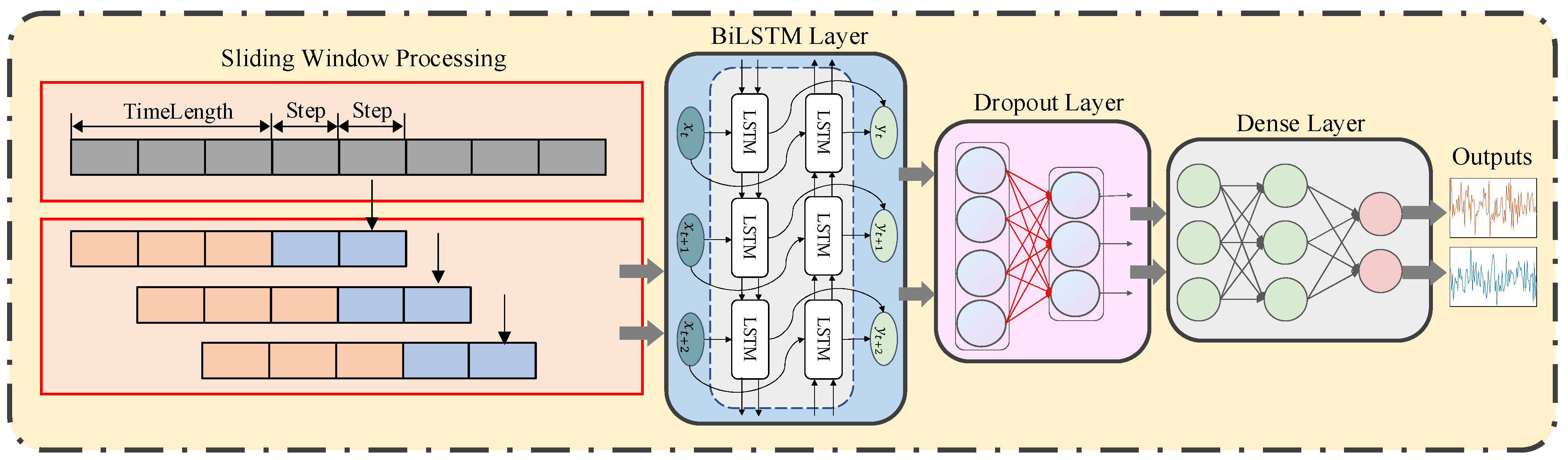
To enable the accurate prediction of vessel attitude under complex sea states, we propose a hierarchical, deep learning-based forecasting module that predicts future roll and pitch from historical measurements. The forecasts provide feed-forward compensation to the wave compensation control system, thereby mitigating performance degradation due to system delays. The overall workflow of the proposed module is shown in Figure 3 and Algorithm 1. First, raw attitude and control data are collected for training, including roll, pitch and yaw measurements and the rotational speeds of the catamaran’s twin propulsion motors. These time series data are preprocessed using a sliding-window scheme to form fixed-length sequences, enabling the model to capture both short-term dynamics and long-term trends.

Subsequently, the sample sequences are fed into a two-layer BiLSTM network, in which the forward and backward subnetworks extract temporal dependencies in both directions. This bidirectional structure facilitates the joint modeling of historical states and future trends, thereby enhancing the representation capability for nonstationary sequences. After temporal feature extraction, a dropout layer is introduced to reduce the network complexity and mitigate overfitting, improving the model’s generalization performance. Finally, a fully connected layer performs nonlinear mapping and fusion of the extracted features to generate the predicted roll and pitch angles of the vessel.

To enhance the training efficiency and generalization capability of the BiLSTM network, a set of optimization strategies is employed during the training process. Specifically, the Adam optimizer is adopted to achieve a favorable balance between convergence speed and numerical stability. The learning rate is fixed throughout training to avoid potential disturbances to the convergence process caused by frequent learning rate adjustments, thereby ensuring stable and smooth training behavior. To mitigate overfitting, dropout layers are incorporated, and an early stopping strategy based on the validation loss is applied. Furthermore, the batch size and the number of training epochs are carefully selected according to the dataset scale and the convergence characteristics of the model, enabling the network to sufficiently capture the nonlinear mapping between inputs and outputs while maintaining good generalization performance and real-time applicability.

Algorithm 1. Deep Learning-Based Attitude Prediction Algorithm

3.2.2. Principle of the Bidirectional Long Short-Term Memory Network

As a special type of recurrent neural network architecture, the Recurrent Recursive Network (RRN) is capable of modeling temporal sequence dependencies from historical data and can effectively capture the intrinsic correlations between different time steps within a known sequence, thereby enabling the accurate prediction of future sequences [42]. By contrast, the BiLSTM specifically addresses the technical bottleneck that plagues traditional unidirectional recurrent neural networks, namely their inability to capture contextual information [43]. Owing to this distinctive advantage, BiLSTM has been widely adopted in a wide range of time series forecasting tasks. This network is composed of two independent LSTM subnetworks, and its working mechanism is as follows: first, the time series data are fed sequentially into the forward LSTM layer, which processes the sequence information frame by frame from front to back and outputs forward-oriented features; subsequently, the same set of data is input into the backward LSTM layer, which parses the sequence in a reverse direction from back to front and extracts backward-oriented features [44]. The final output of the network at each time step is generated by concatenating and fusing the forward and backward feature information, thus yielding more comprehensive and complete contextual features of the sequence [45]. The detailed calculation process of the forward LSTM is given by the following equations:

$${\overrightarrow{h}}_t=H({\omega }_1{x}_t+{\omega }_2{\overrightarrow{h}}_{t-1}+\overrightarrow{b})$$

(17)

where ${\overrightarrow{h}}_t$ denotes the forward hidden state at time step $t$, $x_t$ is the input vector at time step $t$, ${\omega }_1$ represents the weight matrix mapping the input to the hidden state, ${\omega }_2$ is the recurrent weight matrix of the forward hidden state, $\overrightarrow{b}$ denotes the bias vector for forward propagation, and $H$ is the activation function. The computational process of the backward LSTM is expressed as follows:

$${\overleftarrow{h}}_t=H({\omega }_3{x}_t+{\omega }_5{\overleftarrow{h}}_{t+1}+\overleftarrow{b})$$

(18)

where ${\overleftarrow{h}}_t$ represents the backward hidden state at time step $t$, ${\omega }_3$ is the weight matrix mapping the input to the hidden state, ${\omega }_5$ is the recurrent weight matrix of the backward hidden state, $\overleftarrow{b}$ denotes the bias vector for backward propagation, and the computation of the output layer is given as follows:

$$y_t={\omega }_4{\overrightarrow{h}}_t+{\omega }_6{\overleftarrow{h}}_t+b_y$$

(19)

where $y_t$ denotes the output at time step $t$, ${\omega }_4$ and ${\omega }_6$ are the weight matrices connecting the forward and backward hidden states to the output, respectively, and $b_y$ is the bias vector of the output layer.

3.3. Cascaded Disturbance Rejection Control Algorithm for Wave Compensation

As revealed by the Stewart platform’s kinematic equations, the system is inherently a highly nonlinear dynamical system, subject to both exogenous disturbances (e.g., waves and currents) and endogenous perturbations (e.g., actuator nonlinearities). These factors markedly increase the complexity of modeling and control, imposing stringent requirements on accuracy and stability. To address this, we design a cascaded disturbance rejection control module in which ADRC provides attitude compensation, while a velocity loop enhances dynamic performance and robustness. Working in concert, the two ensure a high precision tracking and stable compensation of the Stewart platform under complex sea states. The control procedure is illustrated in Algorithm 2.

Algorithm 2. Cascaded Disturbance Rejection Control Algorithm for Wave Compensation

3.3.1. ADRC-Based Stewart Platform Controller

As revealed by the kinematic formulation, the shipborne Stewart platform is a strongly nonlinear dynamical system subject to substantial exogenous disturbances and internal uncertainties, both of which constrain control accuracy and stability. To address this, we propose an ADRC-based actuator position control scheme comprising a tracking differentiator (TD), a nonlinear state-error feedback (NLSEF) controller, and an extended state observer (ESO) [46]. The ESO provides a real-time estimation of the lumped disturbance, encompassing both internal and external effects, while the nonlinear feedback compensator adapts the control gains to the error magnitude, thereby improving accuracy for small errors and preserving robustness and steady-state stability for large errors.

The tracking differentiator is designed to smooth and differentiate the system input in the presence of abrupt changes, noise, or discontinuities, providing a continuous and smooth reference trajectory for the NLSEF while estimating the input rate of change to improve dynamic performance. The state update equations of the TD are given as follows:

$$\begin{array}{l}\left\{\begin{array}{l}{r}_1(k+1)=r_1(k)+h{r}_2(k)\\ r_2(k+1)=r_2(k)+h\mathrm{fst}(r_1(k)-v(k),r_2(k),{\delta }_1,h)\end{array}\right.\\ \mathrm{fst}(e,\dot{e},{\delta }_1,h)=\left\{\begin{array}{l}-{\displaystyle \frac{e}{{\delta }_1}},\left|e\right|\le {\delta }_1\\ -\mathrm{sign}(e),\left|e\right|>{\delta }_1\end{array}\right.\end{array}$$

(20)

where $r_1(k)$ denotes the position tracking state at time step $k$, $r_2(k)$ represents the velocity tracking state, $v(k)$ is the input signal, $h$ is the sampling period, $\delta$ determines the tracking speed, and $\mathrm{fst}$ is the optimal control synthesis function. $e$ denotes the tracking error, $\dot{e}$ denotes the estimated first-order derivative of the tracking error, and $\mathrm{sign}$ denotes the signum function. The NLSEF controller generates the control law based on system state errors to drive the Stewart platform output to follow the reference input, achieving high precision error regulation through nonlinear combinations. The control law is expressed as follows:

$$\begin{array}{l}u={\beta }_1\mathrm{fal}(e_1,{\alpha }_1,{\delta }_2)+{\beta }_2\mathrm{fal}(e_2,{\alpha }_2,{\delta }_2)\\ \mathrm{fal}(\xi ,{\alpha }_{\mathrm{i}},\delta )=\left\{\begin{array}{l}{\displaystyle \frac{\xi }{{\delta }^{1-{\alpha }_{\mathrm{i}}}}},\left|\xi \right|\le \delta \\ {\left|e\right|}^{{\alpha }_{\mathrm{i}}}\mathrm{sign}(\xi ),\left|\xi \right|>\delta \end{array}\right.\end{array}$$

(21)

where ${\beta }_1$ and ${\beta }_2$ are nonlinear gain coefficients, ${\alpha }_1$ and ${\alpha }_2$ are nonlinear exponents, $\delta$ is the linear-region threshold, respectively, $\mathrm{fal}$ is the nonlinear error feedback function, $\xi$ denotes a generic scalar error variable, ${\alpha }_{\mathrm{i}}$ denotes the nonlinear exponent parameter of the $\mathrm{fal}$ function, and $e_1$ and $e_2$ denote the position and velocity errors; the detailed computation is given by the following equation:

$$\left\{\begin{array}{l}{e}_1=x(t)-x_d(t)\\ e_2=\dot{x}(t)-{\dot{x}}_d(t)\end{array}\right.$$

(22)

where $x(t)$ and $\dot{x}(t)$ represent the system’s actual position and velocity, while $x_d(t)$ and ${\dot{x}}_d(t)$ denote the corresponding desired reference position and velocity signals, and $t$ stands for the time variable.

The ESO is the core of ADRC. It estimates the system states (position and velocity) and, unlike classical observers, augments the state with a lumped disturbance for real-time estimation. The resulting estimates are fed back to achieve closed-loop disturbance compensation. The ESO dynamics are given as follows:

$$\left\{\begin{array}{l}{z}_1(k)=z_1(k-1)+h(z_2(k-1)-{\beta }_3{e}_1)\\ z_2(k)=z_2(k-1)+h(z_3(k-1)-{\beta }_4\mathrm{fal}(e_1,{\alpha }_1,\delta )+bu(k))\\ z_3(k)=z_3(k-1)-h{\beta }_5\mathrm{fal}(e_2,{\alpha }_2,\delta )\end{array}\right.$$

(23)

where $h$ is the system sampling period, $z_1$ denotes the estimated output state, $z_2$ is the estimated derivative of the output, $z_3$ represents the estimated total disturbance, ${\beta }_1$, ${\beta }_2$, and ${\beta }_3$ are the observer gain coefficients, $b$ is the estimated system control gain, $y(k)$ is the actual system output, and $u(k)$ is the control input.

3.3.2. Cascaded Proportional Velocity Control

Building on the position accuracy afforded by ADRC, we introduce a velocity control loop to improve dynamic response and stability under disturbances. By continuously monitoring the platform velocity and injecting an additional damping term proportional to the velocity error, the system’s damping characteristics are enhanced, thereby reducing overshoot and suppressing oscillations induced by external disturbances. Specifically, the velocity loop adopts a proportional controller, expressed as follows:

$$u_{\nu }=-k_p{e}_2$$

(24)

where $u_v$ denotes the control output, $e_2$ represents the velocity error, and $k_p>0$ is the proportional gain coefficient. The physical interpretation of this law is that, when the platform velocity deviates from the reference value, an ‘additional damping force’ proportional to the deviation is applied via the proportional gain, thereby increasing the system’s response speed, improving overall stability, and effectively suppressing disturbance-induced overshoot and oscillations.

3.3.3. System Stability Analysis

The closed-loop stability of the proposed control strategy is analyzed from three aspects: system boundedness, convergence of the ESO, and selection of the velocity-proportional gain $k_p$. First, under the assumption that external disturbances and model uncertainties are bounded, and considering that the control inputs are subject to the physical saturation constraints of the actuators, all system state variables remain bounded. The baseline feedback controller guarantees the basic attitude stability of the platform, while the compensation control module suppresses wave-induced disturbances without introducing unbounded control inputs. Therefore, the overall closed-loop system satisfies the bounded-input bounded-output (BIBO) stability condition, and no divergence of system states occurs.

To estimate the total disturbance and unmodeled dynamics, the ESO parameters are designed using the commonly adopted bandwidth-based tuning method in ADRC theory. The observer gains ${\beta }_3$, ${\beta }_4$, and ${\beta }_5$ are parameterized by the observer bandwidth ${\omega }_{\mathrm{b}}$ as follows:

$${\beta }_3=3{\omega }_{\mathrm{b}},{\beta }_4=3{\omega }_{\mathrm{b}}^2,{\beta }_5={\omega }_{\mathrm{b}}^3$$

(25)

With the above parameter configuration, the characteristic polynomial of the ESO is a Hurwitz polynomial, which guarantees the exponential convergence of the observer estimation error under ideal conditions. In the presence of bounded disturbances and modeling errors, the observer estimation error remains uniformly ultimately bounded (UUB).

In the velocity-proportional control loop, the proportional gain $k_p$ directly affects the dynamic response and stability margin of the closed-loop system. An excessively small $k_p$ leads to a sluggish system response, whereas an excessively large $k_p$ may amplify measurement noise or excite unmodeled high-frequency dynamics, potentially causing oscillations or instability. In this study, $k_p$ is selected according to the principle of ensuring a sufficient stability margin while maintaining a satisfactory dynamic performance. Its value is determined through simulation-based tuning to lie within a stable operating region. Under the selected gain, the platform operates stably without sustained oscillations or divergence.

By jointly considering system boundedness, the convergence properties of the ESO, and the appropriate selection of the velocity-proportional gain $k_p$, it can be concluded that the proposed control scheme achieves closed-loop stability. Simulation results further confirm that the system maintains a stable operation under various operating conditions and disturbance scenarios.

4. Results and Discussion

4.1. Experimental Settings

The experiments were conducted in MATLAB/Simulink R2023a, in which a complete dynamic model of the Stewart platform was developed using a Simscape multibody. This model accurately captures the spatial motion characteristics of the platform and the dynamic behavior of its actuators. Furthermore, a three-dimensional visualization of platform attitude variations and actuator motions is realized through the mechanics explorer, enabling the intuitive illustration and dynamic verification of the attitude compensation process. The main simulation parameters and the hyperparameter settings of the prediction model are summarized in

Table 1. Experimental parameter settings.

Simulink R2023a		Predication Model
Total simulation time	10 s	Parameters	Value
Fixed step size	0.01 s	Learning rate	0.015
Prediction sampling time	0.1 s	Epochs	200
Solver type	Fixed-step	Batch size	256
Solver	Ode14x	Optimizer	Adam
Controller sampling time	0.01 s	Dropout rate	0.05
Zero-crossing detection	Disabled	Neurons	64

.

To quantitatively evaluate system performance, different error metrics are employed to assess the neural network prediction accuracy and the effectiveness of wave-induced attitude compensation, respectively. For neural network prediction performance evaluation, four commonly used metrics, the mean squared error (MSE), root mean squared error (RMSE), mean absolute error (MAE), and mean absolute percentage error (MAPE), are adopted to quantify the prediction accuracy and stability of roll and pitch motions. For wave-induced attitude compensation performance evaluation, the root mean squared error (RMSE), mean absolute error (MAE), mean error (ME), and relative error (RE) are further utilized to comprehensively assess the compensation effectiveness for roll and pitch motions.

$$\mathrm{MSE}={\displaystyle \frac{1}{n}}{\displaystyle \sum _{i=1}^n{(y_i-{\widehat{y}}_i)}^2}$$

(26)

$$\mathrm{RMSE}=\sqrt{{\displaystyle \frac{1}{n}}{\displaystyle \sum _{i=1}^n{(y_i-{\widehat{y}}_i)}^2}}$$

(27)

$$\mathrm{MAE}={\displaystyle \frac{1}{n}}{\displaystyle \sum _{i=1}^n\left|y_i-{\widehat{y}}_i\right|}$$

(28)

$$\mathrm{MAPE}={\displaystyle \frac{100\%}{n}}{\displaystyle \sum _{i=1}^n\frac{\left|y_i-{\widehat{y}}_i\right|}{\left|y_i\right|}}$$

(29)

$$\mathrm{ME}={\displaystyle \frac{1}{n}}{\displaystyle \sum _{i=1}^n(y_i-{\widehat{y}}_i)}$$

(30)

$$\mathrm{RE}={\displaystyle \frac{\left|y_i-{\widehat{y}}_i\right|}{\left|y_i\right|}}\times 100\%$$

(31)

The corresponding formulations of these error metrics are presented below. In the evaluation of neural network prediction performance, $y_i$ denotes the true attitude value at the i-th sampling instant, and ${\widehat{y}}_i$ represents the attitude predicted by the neural network. In the evaluation of wave-induced attitude compensation performance, $y_i$ denotes the actual output after attitude compensation, while ${\widehat{y}}_i$ represents the reference value of the desired attitude. Here, $n$ denotes the total number of samples used for error calculation.

4.2. Sea State Simulation Cases

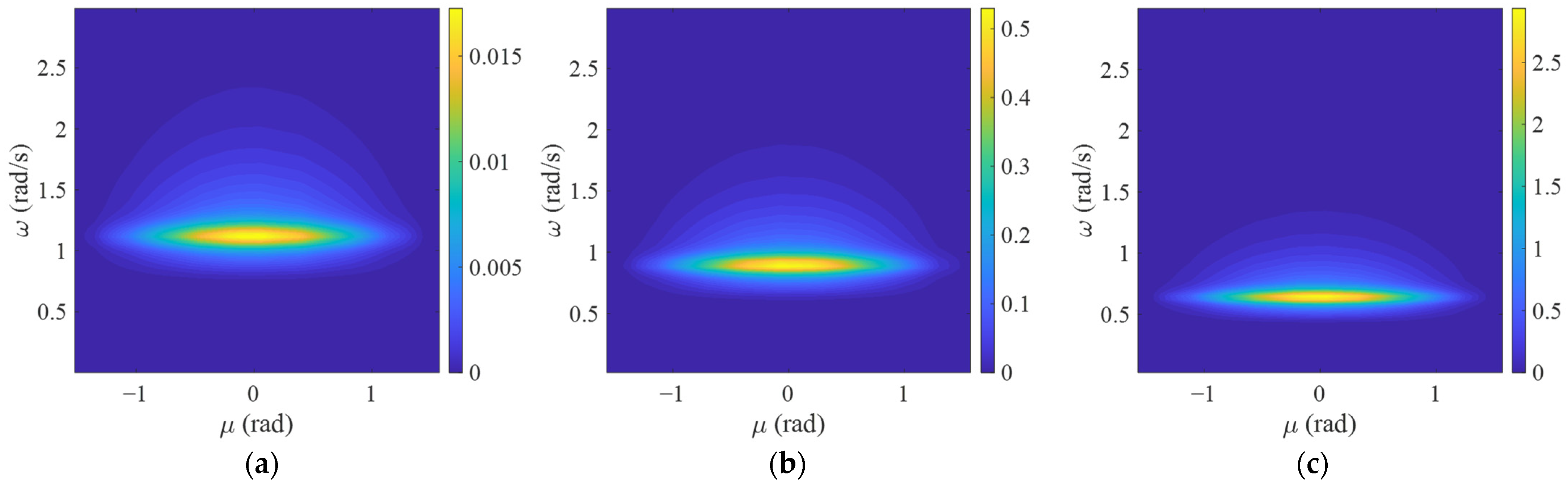
To comprehensively evaluate the performance of the control algorithm under ocean disturbances of varying intensities, three representative sea states, sea state 2, sea state 4, and sea state 6, were selected as experimental scenarios. The simulations were conducted using the catamaran dynamic model established in Section 3.1. To reproduce these sea states, the corresponding JONSWAP wave spectrum parameters, summarized in

Table 2. Operating condition parameters.

Case Number	Sea State	${\mathit{H}}_{\mathbf{s}}$	${\mathit{T}}_{\mathbf{z}}$	$\mathsf{\gamma }$
Case 1	Sea state 2	0.5 m	4 s	3.3
Case 2	Sea state 4	2 m	5 s	3.3
Case 3	Sea state 6	5 m	7.2 s	3.3

, were employed to generate the wave disturbances. In this table, $H_{\mathrm{s}}$ denotes the significant wave height, $T_{\mathrm{z}}$ represents the mean zero-crossing period, and $\gamma$ is the peak enhancement factor. As illustrated in Figure 4, two-dimensional directional wave spectra were generated for each sea state to characterize the distribution of wave energy in both frequency and direction.

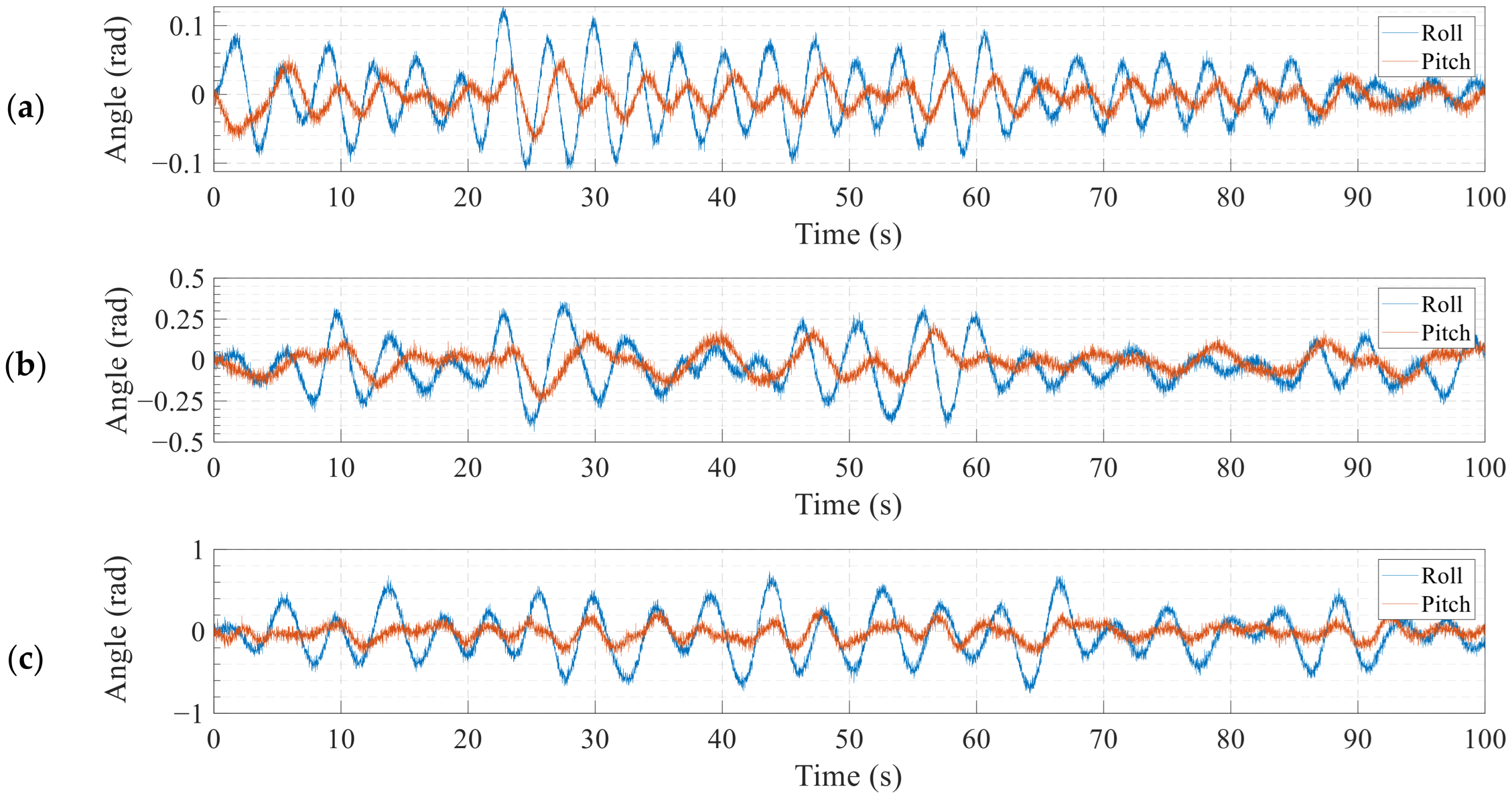
To visually illustrate the vessel motion characteristics under different sea conditions, Figure 5 presents the roll and pitch attitude response curves for the three considered sea states.

As shown in Figure 5, the time histories of roll and pitch motions exhibit pronounced differences across sea conditions. Statistical analysis of the signal amplitudes enables a quantitative characterization of the vessel’s attitude response under each sea state. Under sea state 2 conditions, the vessel is subjected to only mild wave disturbances, resulting in small variations in roll and pitch angles. Specifically, roll fluctuations are within approximately ±0.12 rad, while pitch fluctuations remain within ±0.05 rad. The attitude response is dominated by low-frequency, small-amplitude oscillations, indicating relatively stable vessel motion and limited attitude disturbances under low-energy sea conditions. When the sea state increases to 4, attitude fluctuations become significantly larger, with roll amplitudes increasing to approximately ±0.25 rad and pitch amplitudes to about ±0.16 rad. The motion signals exhibit higher frequencies and noticeable asymmetry, indicating that, under moderate sea conditions, wave excitation in the roll direction is more pronounced, whereas the pitch response remains relatively weaker. This behavior places higher demands on the dynamic response capability of the control system. Under sea state 6 conditions, the vessel’s attitude fluctuations intensify further, with roll amplitudes reaching up to ±0.6 rad and pitch amplitudes increasing to approximately ±0.22 rad. The attitude signals exhibit high-frequency, intense, and irregular oscillations, indicating that, under severe sea conditions, wave disturbances have a substantially amplified impact on vessel motion, with roll becoming the dominant mode of motion.

4.3. Wave Compensation Experiment

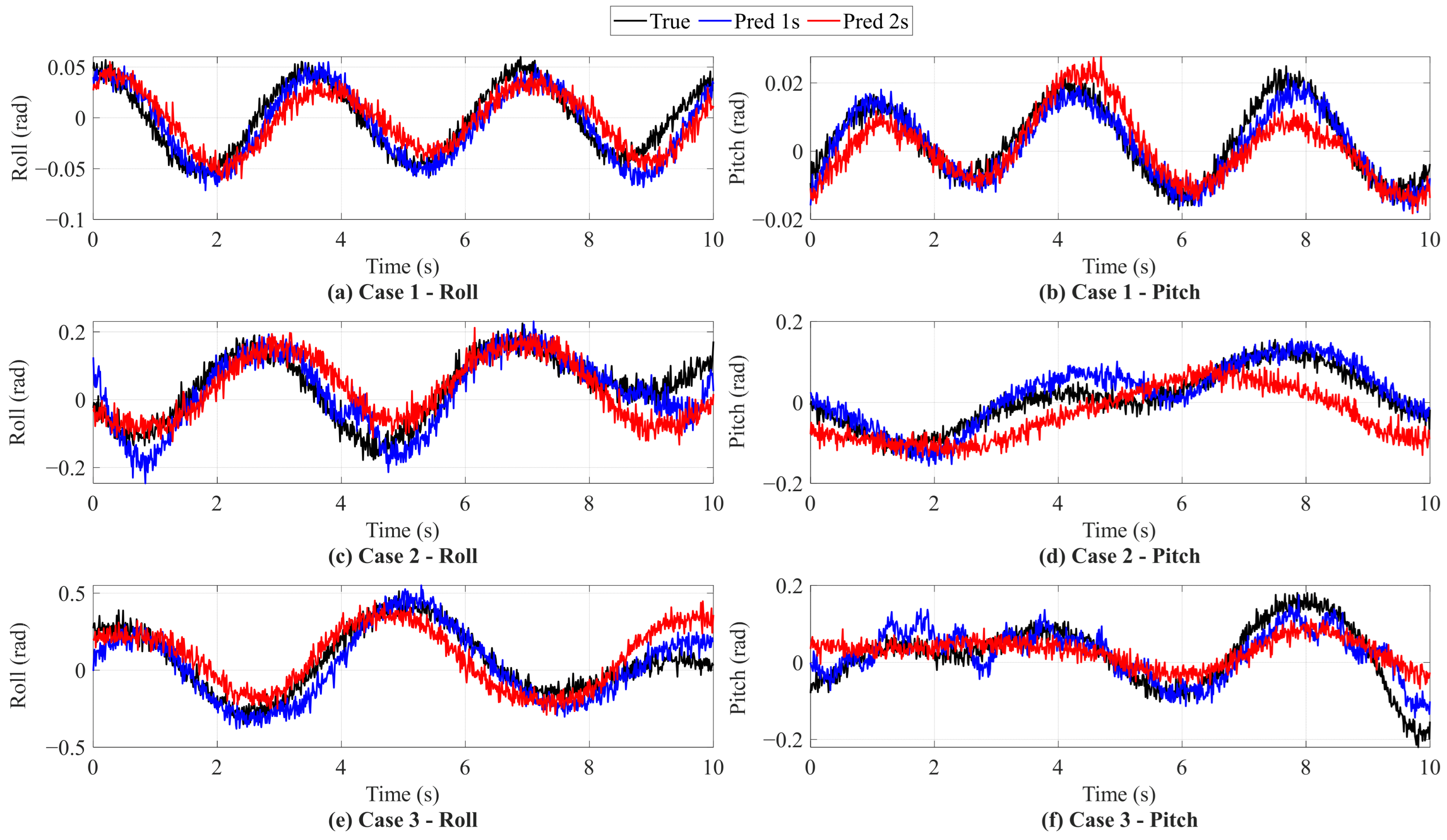
Based on the ship attitude data obtained in Section 4.2, the prediction model adopts a multivariate time series modeling approach. By comprehensively considering the sampling and filtering of attitude sensors, the computation of online prediction and control algorithms, and the dynamic response of actuators, an inevitable overall time delay is introduced in the sensing, computation, and actuation processes, with a magnitude of approximately 1 s. To investigate the influence of the prediction horizon on performance, comparative prediction experiments with horizons of 1 s and 2 s were conducted, and the corresponding results are presented in Figure 6 and

Table 3. Error evaluation index of roll.

Case	Case 1		Case 2		Case 3
Pred-Time	Pred 1 s	Pred 2 s	Pred 1 s	Pred 2 s	Pred 1 s	Pred 2 s
MSE	0.00018	0.00030	0.00228	0.00314	0.00504	0.00852
RMSE	0.01330	0.01735	0.04773	0.05605	0.07096	0.09233
MAE	0.01091	0.01529	0.03727	0.04312	0.05550	0.07882
MAPE	0.20400	0.28598	0.22339	0.25848	0.12926	0.18357

and

Table 4. Error evaluation index of pitch.

Case	Case 1		Case 2		Case 3
Pred-Time	Pred 1 s	Pred 2 s	Pred 1 s	Pred 2 s	Pred 1 s	Pred 2 s
MSE	0.00001	0.00004	0.00074	0.00296	0.00229	0.00267
RMSE	0.00307	0.00609	0.02712	0.05441	0.04781	0.05165
MAE	0.00244	0.00496	0.02213	0.04644	0.03860	0.04184
MAPE	0.11581	0.23535	0.17884	0.37529	0.20663	0.27134

. It can be observed that, under all operating conditions, increasing the prediction horizon from 1 s to 2 s leads to varying degrees of error growth, indicating that a longer prediction horizon significantly degrades the prediction accuracy. In contrast, the 1 s prediction consistently achieves smaller error values across all cases, demonstrating a superior prediction accuracy and stability. Moreover, as the operating conditions become more severe from Case 1 to Case 3, the overall prediction errors exhibit an increasing trend, and the performance degradation caused by the extended prediction horizon becomes more pronounced. Therefore, this study employs historical attitude information over the past 5 s to perform a 1 s ahead prediction of ship attitude variations.

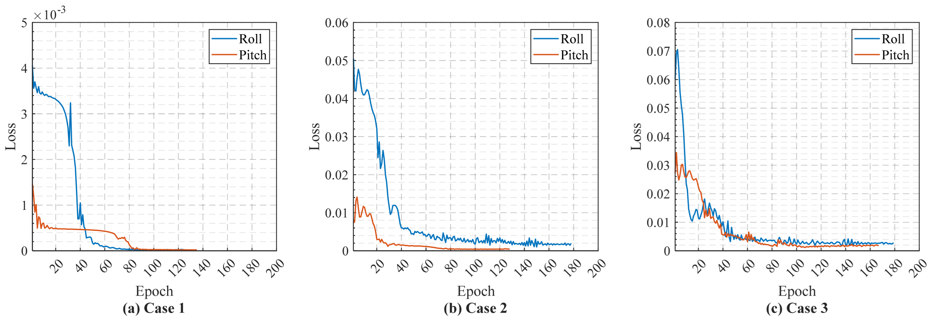
The input variables of the model include the ship’s roll, pitch, and yaw angles, while the rotational speeds of the port and starboard propulsion motors are incorporated as control inputs. Together, these variables form a multidimensional time series input. The dataset is divided chronologically into training, validation, and test sets, with proportions of 60%, 20%, and 20%, respectively. To enhance the generalization capability and suppress overfitting, dropout layers are introduced during network training, and an early stopping strategy based on the validation loss is employed, ensuring that the model maintains a high prediction accuracy while exhibiting a robust and stable performance. Figure 7 illustrates the convergence curves of the validation loss under three operating conditions. It can be observed that, across all conditions, the validation loss decreases progressively with training epochs and eventually converges, indicating favorable convergence properties and training stability of the proposed prediction model. Although variations in convergence speed and final loss levels are observed among different operating conditions—primarily due to differences in attitude amplitudes and dynamic characteristics—the validation loss does not exhibit noticeable rebound or oscillation. This confirms that no significant overfitting occurs during training and that the model demonstrates a strong generalization capability.

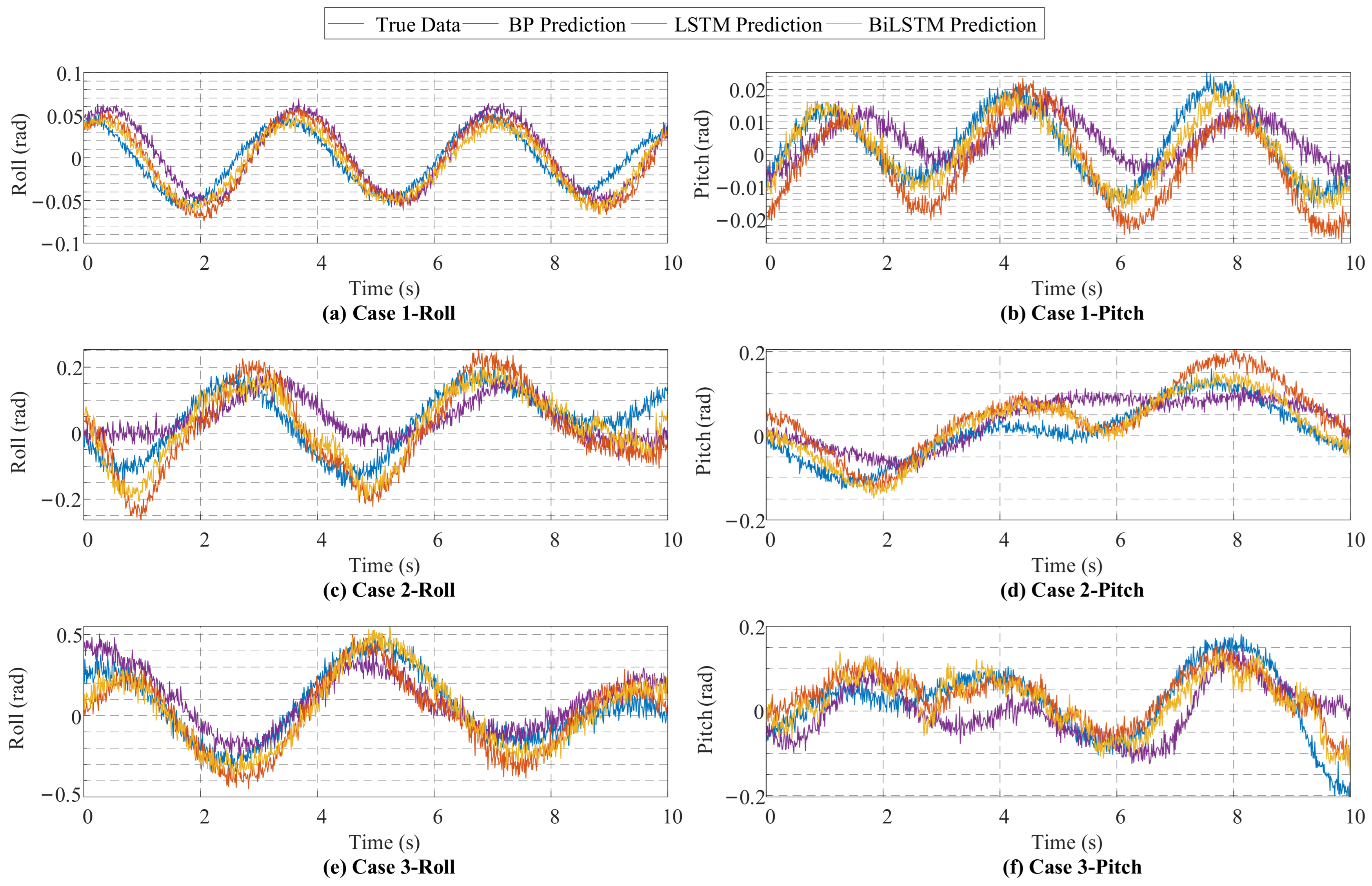
Figure 8 compares the predicted and actual roll and pitch responses under three operating conditions. BP neural networks are able to capture the overall periodic trends of ship attitude variations; however, they exhibit noticeable deviations in phase consistency and peak amplitude representation. In particular, under highly fluctuating conditions, significant amplitude attenuation and local distortion can be observed. The results indicate that, across all cases, both the LSTM and BiLSTM models successfully capture the overall trends of vessel attitude variations. However, the BiLSTM model demonstrates a superior performance in terms of phase consistency and peak-tracking accuracy. In particular, in Case 2 and Case 3, as the sea state intensity increases and the vessel motion exhibits stronger nonlinear characteristics, owing to the lack of explicit modeling for temporal dependencies, the prediction errors of the BP network are further amplified in the vicinity of local extrema, the LSTM model shows noticeable lag and amplitude deviations near local extrema, and the BiLSTM model maintains a better dynamic responsiveness. These observations suggest that under complex wave excitation, vessel attitude signals exhibit pronounced temporal correlations and non-stationary behavior. By simultaneously exploiting forward and backward temporal information, the BiLSTM model provides a more comprehensive representation of attitude evolution, resulting in an enhanced modeling capability and prediction stability under highly dynamic conditions.

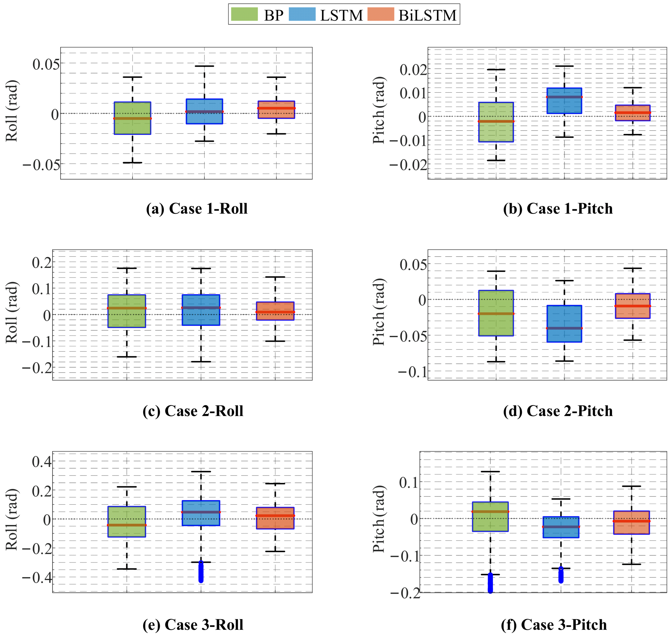
Figure 9 illustrates the boxplot distributions of prediction errors for the three operating conditions. In Case 1, the error distribution of the BP neural network is more dispersed than that of the sequence-based models, with both the median error and interquartile range exceeding those of the LSTM and BiLSTM models. The errors of both the BiLSTM and LSTM models are relatively concentrated; nevertheless, the BiLSTM model exhibits a lower median and narrower interquartile range than the LSTM model, indicating smaller average errors, reduced variability, and superior prediction stability, with almost no outliers. As the sea state increases to Case 2, the error distributions expand noticeably. The boxplot of the BP network exhibits a wider interquartile range and longer whiskers, indicating its limited capability to adapt to instantaneous attitude variations under non-stationary wave excitations. The LSTM model exhibits a greater number of outliers, indicating larger prediction errors in certain time intervals. In contrast, the BiLSTM model maintains a more compact interquartile range with more concentrated errors, consistent with the reductions in RMSE and MAE reported in

Table 5. Error evaluation index of roll.

Case	Case 1			Case 2			Case 3
Model	BiLSTM	LSTM	BP	BiLSTM	LSTM	BP	BiLSTM	LSTM	BP
MSE	0.00018	0.00033	0.00038	0.00228	0.00529	0.00609	0.00504	0.00961	0.01135
RMSE	0.01330	0.01813	0.01954	0.04773	0.07274	0.07807	0.07096	0.09805	0.10652
MAE	0.01091	0.01471	0.01658	0.03727	0.06310	0.06530	0.05550	0.08269	0.09497
MAPE	0.20400	0.27523	0.31005	0.22339	0.37818	0.39141	0.12926	0.19259	0.22119

and

Table 6. Error evaluation index of pitch.

Case	Case 1			Case 2			Case 3
Model	BiLSTM	LSTM	BP	BiLSTM	LSTM	BP	BiLSTM	LSTM	BP
MSE	0.00001	0.00008	0.00009	0.00074	0.00232	0.00208	0.00229	0.00342	0.00687
RMSE	0.00307	0.00898	0.00962	0.02712	0.04820	0.04561	0.04781	0.05851	0.08290
MAE	0.00244	0.00767	0.00846	0.02213	0.04192	0.03883	0.03860	0.04177	0.06707
MAPE	0.11581	0.36375	0.40102	0.17884	0.33872	0.31379	0.20663	0.22355	0.35900

. In Case 3, although the error dispersion of all three models increases further, the BiLSTM model still clearly outperforms both the LSTM and BP networks, exhibiting a lower median error and fewer outliers, which demonstrates the superior disturbance rejection capability of the bidirectional architecture under highly uncertain conditions. A more stable error distribution is beneficial for maintaining smooth control inputs, thereby improving the performance of practical compensation control.

To quantitatively evaluate the prediction accuracy, Table 5 shows that, for the roll prediction task, the BiLSTM model achieves significantly lower error metrics than both the LSTM and BP neural networks across all three sea states. For instance, in Case 3, the RMSE and MAE of the BiLSTM are reduced by approximately 30% and 25%, respectively, compared with those of the LSTM, while the reductions relative to the BP network are even more pronounced. This indicates that the bidirectional architecture is more effective in suppressing prediction errors under strong wave disturbances. Similar conclusions can be drawn from the pitch prediction results in Table 6. Although pitch motion exhibits smaller amplitudes, its dynamics are still strongly influenced by wave coupling effects. Across Case 1 to Case 3, the BiLSTM model consistently achieves lower MSE and RMSE values, with particularly pronounced reductions in MAPE under moderate and high sea states, highlighting its superior control over relative prediction errors.

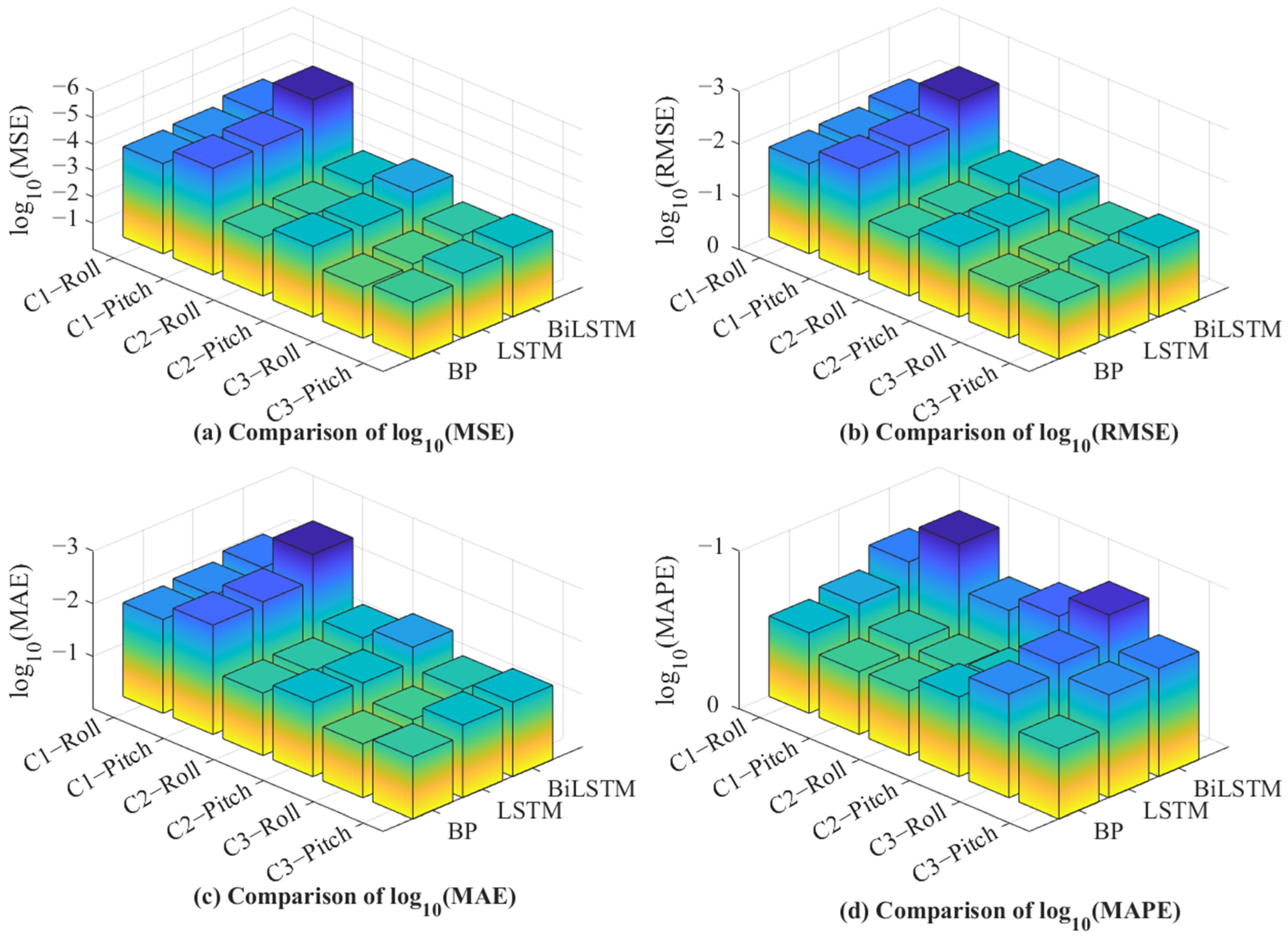
To further illustrate the performance differences among the models, Figure 10 presents evaluation metrics transformed using log₁₀, where smaller values indicate better performance. Across different cases, the BiLSTM model consistently outperforms the conventional LSTM and BP neural networks in all four evaluation metrics, demonstrating a superior prediction accuracy and stability. This confirms that the bidirectional temporal structure more effectively exploits forward and backward dependencies in time series data, thereby enhancing the modeling of complex dynamic behaviors.

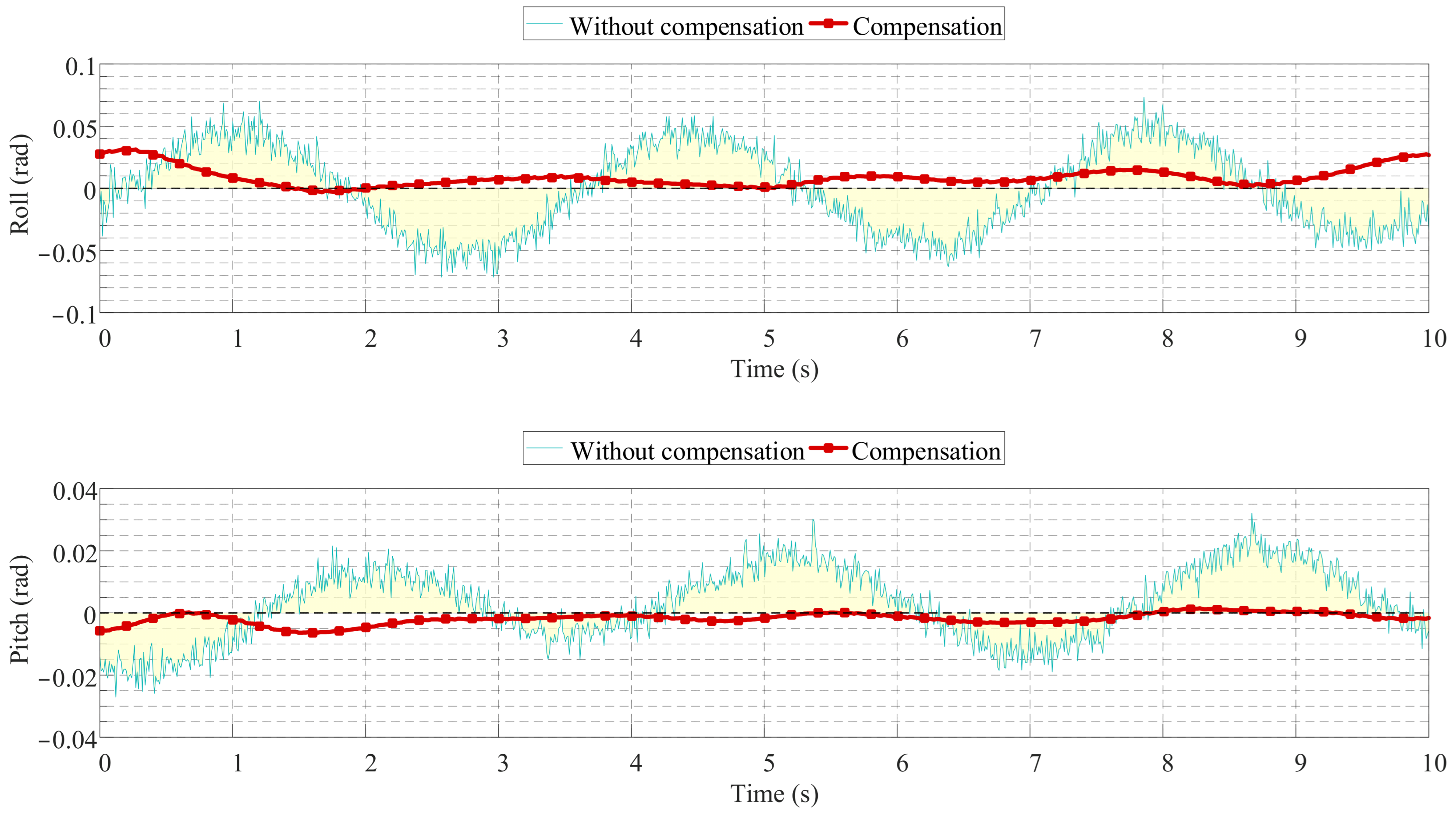
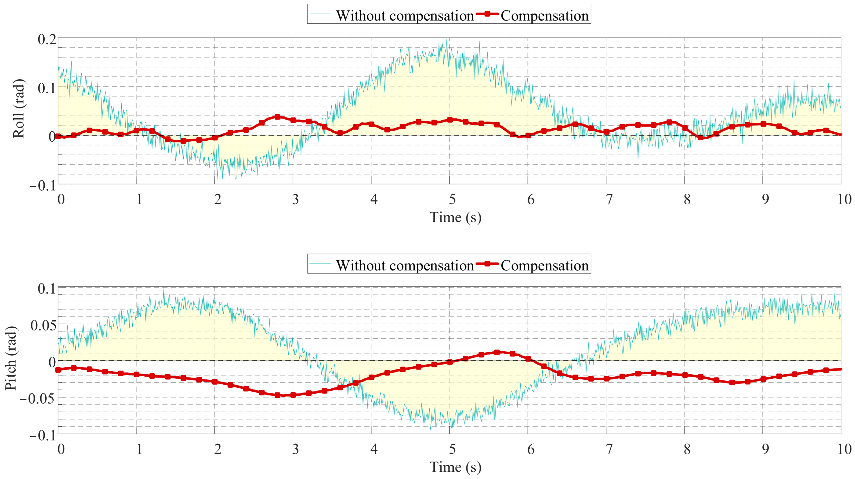
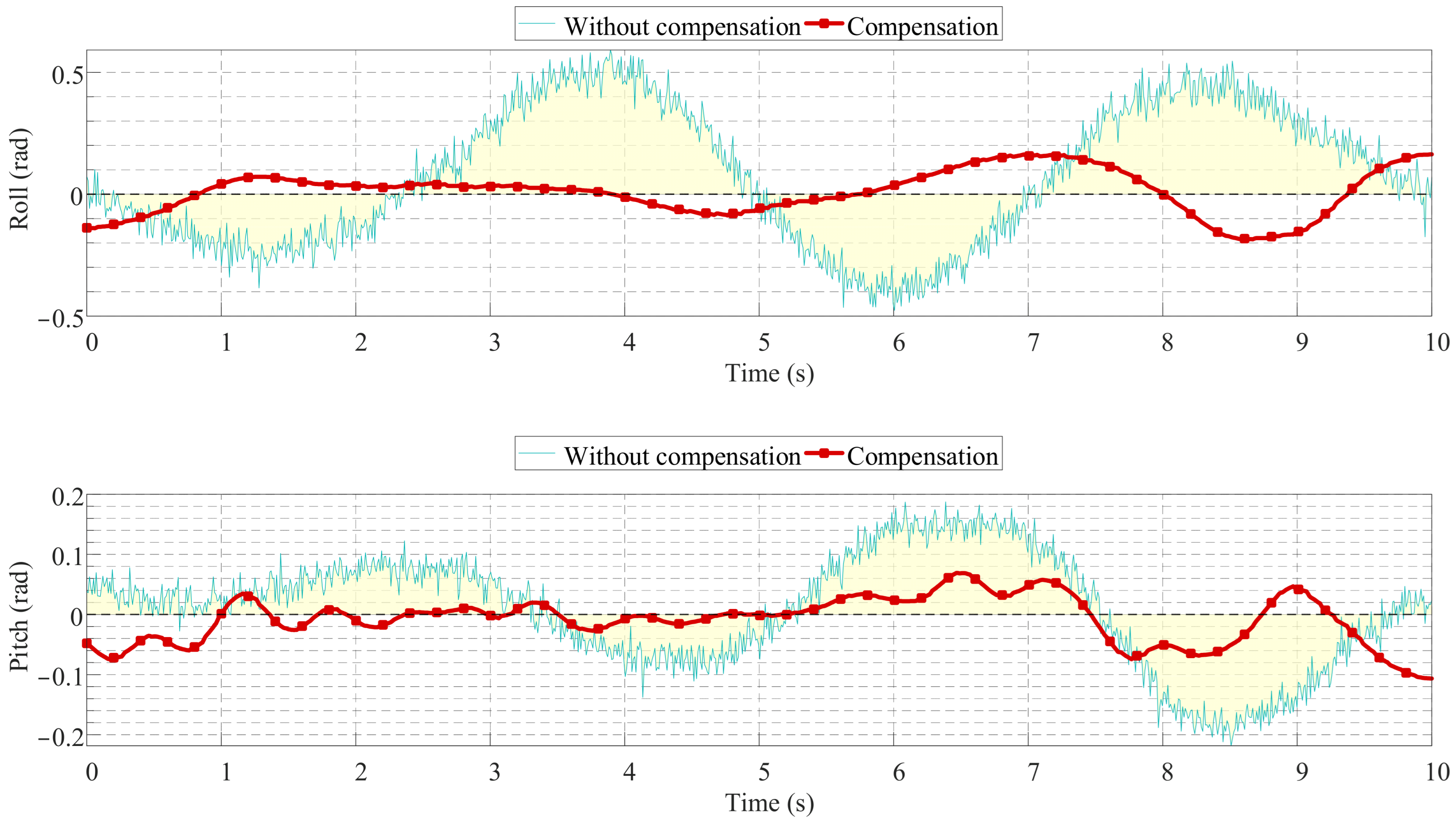
Building upon the attitude prediction results, the predicted information is incorporated into the motion compensation control of the Stewart platform, with the corresponding compensation effects shown in Figure 11, Figure 12 and Figure 13. ‘Without compensation’ represents the platform’s baseline response under identical sea conditions, reflecting its passive behavior in response to wave disturbances. In contrast, ‘With compensation’ describes the system response when a motion compensation strategy, based on predicted attitudes, is implemented. The results demonstrate that predictive compensation significantly suppresses roll and pitch oscillations under all three sea states. In Case 1, although the original motion amplitudes are relatively small, predictive compensation further improves attitude stability, reducing the roll peak from ±0.05 rad to ±0.025 rad and the pitch peak from ±0.02 rad to ±0.01 rad, corresponding to a 50% reduction in both cases. In Case 2, platform attitude disturbances increase substantially and exhibit periodic oscillations in the absence of compensation. After introducing predictive compensation, the roll amplitude is reduced from ±0.17 rad to ±0.04 rad (a 76.4% reduction), and the pitch amplitude is reduced from ±0.12 rad to ±0.05 rad (a 58.3% reduction), indicating a more pronounced compensation effect than in low sea conditions. In Case 3, where platform attitude disturbances are most severe, predictive compensation reduces the roll amplitude from ±0.45 rad to ±0.2 rad (a 55.6% reduction) and the pitch amplitude from ±0.2 rad to ±0.1 rad (a 50% reduction), significantly enhancing the system robustness and disturbance rejection capability. Overall, across all operating conditions, the attitude prediction-based motion compensation strategy for the Stewart platform effectively reduces roll and pitch vibration amplitudes, with increasingly pronounced benefits under harsher sea conditions, thereby providing reliable attitude stabilization for high-precision shipborne equipment.

4.4. Analysis of Compensation Performance of Multiple Models

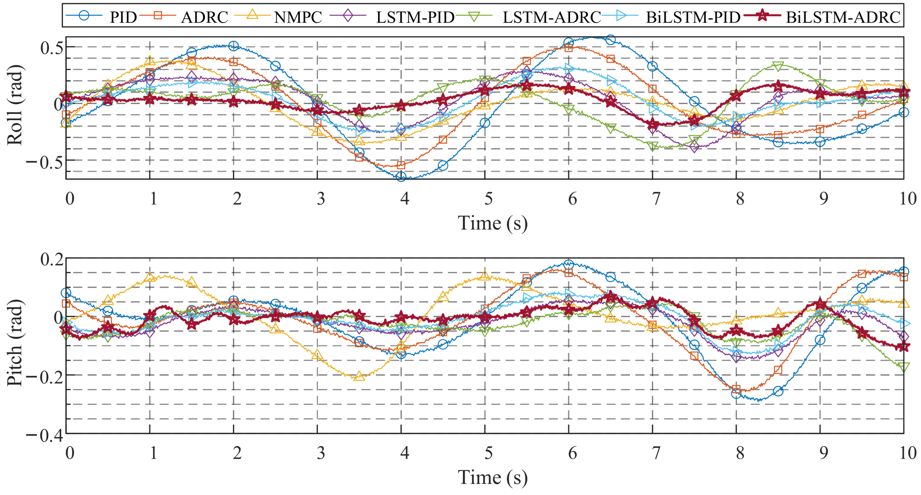
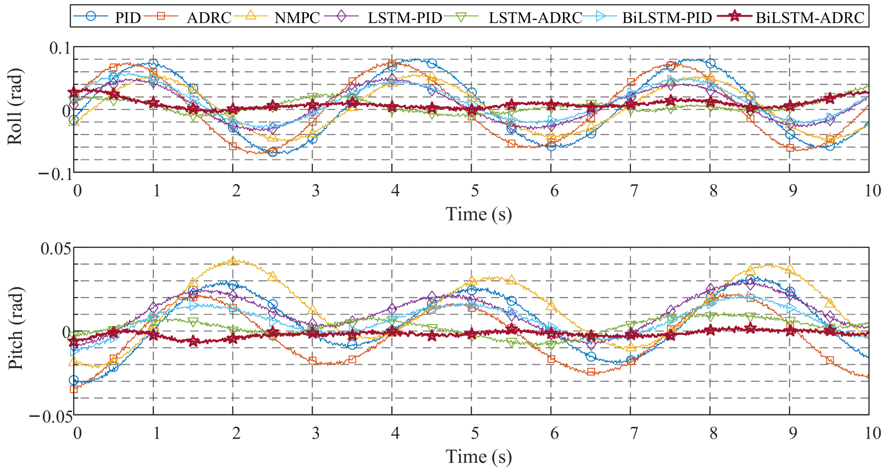
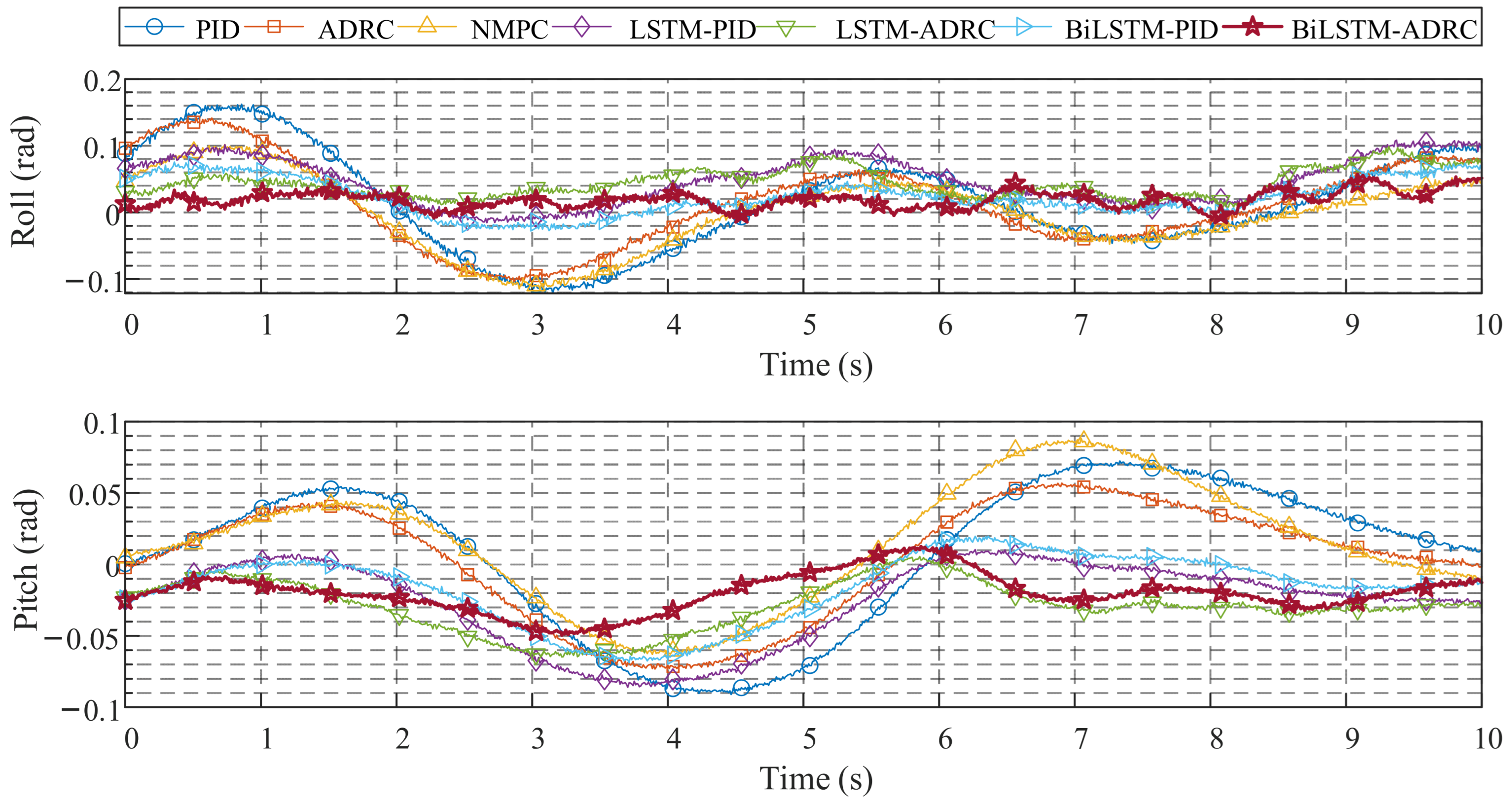
To evaluate the wave compensation performance of different control and predictive compensation strategies under various sea states, this section systematically compares PID, ADRC, Nonlinear Model Predictive Control (NPMC) and several control schemes integrated with LSTM/BiLSTM predictive models. The analysis is based on roll and pitch compensation performance, as illustrated in Figure 14, Figure 15 and Figure 16, and quantitative evaluation metrics, presented in

Table 7. Error evaluation index of Case 1.

	Roll				Pitch
	RMSE	MAE	ME	RE	RMSE	MAE	ME	RE
PID	0.0489	0.0437	0.0790	2.6692	0.0170	0.0147	0.0311	3.0932
ADRC	0.0474	0.0426	0.0737	2.4926	0.0158	0.0141	0.0269	2.6777
NMPC	0.0344	0.0308	0.0539	1.8221	0.0219	0.0178	0.0415	4.1359
LSTM-PID	0.0293	0.0248	0.0521	1.7615	0.0151	0.0128	0.0284	2.8319
LSTM-ADRC	0.0136	0.0096	0.0389	1.3145	0.0058	0.0051	0.0097	0.9651
BiLSTM-PID	0.0272	0.0233	0.0484	1.6339	0.0100	0.0080	0.0201	2.0105
BiLSTM-ADRC	0.0103	0.0081	0.0278	0.9386	0.0024	0.0019	0.0064	0.6372

,

Table 8. Error evaluation index of Case 2.

	Roll				Pitch
	RMSE	MAE	ME	RE	RMSE	MAE	ME	RE
PID	0.0832	0.0710	0.1576	2.5930	0.0460	0.0369	0.0888	2.6126
ADRC	0.0703	0.0598	0.1369	2.2526	0.0378	0.0303	0.0718	2.1113
NMPC	0.0625	0.0529	0.1084	1.7825	0.0412	0.0345	0.0858	2.5207
LSTM-PID	0.0510	0.0425	0.09412	1.5485	0.0414	0.0321	0.0843	2.4778
LSTM-ADRC	0.0406	0.0361	0.08394	1.3810	0.03621	0.0314	0.0633	1.8614
BiLSTM-PID	0.0330	0.0281	0.0696	1.1450	0.0327	0.0265	0.0663	1.9496
BiLSTM-ADRC	0.0195	0.0169	0.0407	0.6700	0.0277	0.0244	0.0480	1.4100

and

Table 9. Error evaluation index of Case 3.

	Roll				Pitch
	RMSE	MAE	ME	RE	RMSE	MAE	ME	RE
PID	0.3670	0.3212	0.6578	2.7444	0.1170	0.0909	0.2841	3.8036
ADRC	0.3021	0.2614	0.5532	2.3077	0.1049	0.0823	0.2524	3.3792
NMPC	0.1886	0.1551	0.3738	1.5145	0.0856	0.0663	0.2065	2.8307
LSTM-PID	0.1877	0.1636	0.3856	1.6086	0.0543	0.0426	0.1410	1.8881
LSTM-ADRC	0.1733	0.1417	0.3876	1.6170	0.0479	0.0358	0.1732	2.3192
BiLSTM-PID	0.1580	0.1322	0.3138	1.3093	0.0507	0.0394	0.1243	1.6640
BiLSTM-ADRC	0.0940	0.0781	0.18534	0.7734	0.0390	0.0299	0.1066	1.4273

.

Under sea state 2, all models maintained system stability, though compensation accuracy varied significantly. In the roll channel, PID and ADRC achieved RMSE values of 0.0489 and 0.0474, respectively, indicating that improvements in the control structure alone offer limited gains under low-disturbance conditions. Incorporating predictive models substantially enhanced compensation accuracy: LSTM-PID and BiLSTM-PID reduced RMSE to 0.0293 and 0.0272, representing an over 40% reduction compared with PID control, with BiLSTM outperforming unidirectional LSTM. The RMSE of NMPC is 0.0344, which outperforms the conventional PID and ADRC controllers but remains slightly higher than that of LSTM/PID-based methods. Overall, BiLSTM-ADRC achieved the best performance, with a roll RMSE of only 0.0103, approximately 79% lower than PID control. In the pitch channel, although the disturbance amplitudes were smaller than in roll, the performance differences remained evident. PID and ADRC RMSE values were 0.0170 and 0.0158, respectively, reflecting residual oscillations. The RMSE of NMPC is 0.0219, performing slightly better than PID/ADRC, still inferior to the predictive models in terms of compensation effectiveness. Predictive compensation further improved performance, with BiLSTM-PID achieving an RMSE of 0.0100. BiLSTM-ADRC demonstrated the highest precision, with an RMSE, MAE, and ME of 0.0024, 0.0019, and 0.0064, respectively, representing an 85.9% reduction relative to PID and highlighting its fine suppression capability for minor attitude fluctuations under weak disturbances.

As disturbance intensity increased to sea state 4, the performance gaps between models widened. In roll, PID and ADRC RMSE increased to 0.0832 and 0.0703, indicating that traditional controllers struggle to mitigate wave-induced uncertainties under moderate disturbances. NMPC achieves an RMSE of 0.0625, representing an improvement over traditional methods, yet it is still higher than that of the predictive approaches. Predictive compensation significantly improved performance, with LSTM-PID and BiLSTM-PID RMSE reduced to 0.0510 and 0.0330, respectively; notably, BiLSTM-PID achieved roughly 40% of the PID RMSE, demonstrating the bidirectional temporal structure’s superior ability to capture critical attitude features under stronger perturbations. BiLSTM-ADRC remained the best-performing scheme, with a roll RMSE of 0.0195 and consistently superior MAE and RE metrics. In the pitch channel, traditional controllers also degraded under stronger disturbances (PID: 0.0460, ADRC: 0.0378), whereas predictive models exhibited a better adaptability. Comparatively, NMPC exhibits an RMSE of 0.0412, which is better than conventional control but not comparable to the predictive models. BiLSTM-PID reduced the pitch RMSE to 0.0327, while BiLSTM-ADRC maintained the lowest errors, with an RMSE and MAE of 0.0277 and 0.0244, representing a 26.7% reduction relative to ADRC and confirming the synergistic effect of predictive compensation with ADRC under moderate disturbances.

In sea state 6, the model performance differences were most pronounced. Traditional PID control in roll reached an RMSE of 0.3670, reflecting significant performance failure; ADRC improved slightly but remained at 0.3021. Under severe sea states, NMPC reduces the RMSE to 0.1886 relative to traditional methods; however, it remains above the values achieved by deep learning-based predictive models. Deep learning-based predictive models showed substantial advantages: LSTM-PID and BiLSTM-PID reduced the RMSE to 0.1877 and 0.1580, achieving an over 50% reduction relative to PID, with BiLSTM better capturing complex, non-stationary attitude dynamics. BiLSTM-ADRC achieved the best overall performance, with a roll RMSE of 0.0940, representing a 74% reduction versus PID, and superior ME and RE values compared with all other models. In pitch, strong wave excitation caused a marked degradation in traditional control (PID: 0.1170, ADRC: 0.1049). Similarly, the RMSE of NMPC is 0.0856, showing moderate compensation performance. Predictive models improved pitch performance substantially, with LSTM-PID and BiLSTM-PID RMSE values of 0.0543 and 0.0507. BiLSTM-ADRC achieved the lowest pitch errors (RMSE: 0.0390, MAE: 0.0299, ME: 0.1066), demonstrating the effective suppression of peak pitch deviations and superior longitudinal attitude stabilization under extreme sea states.

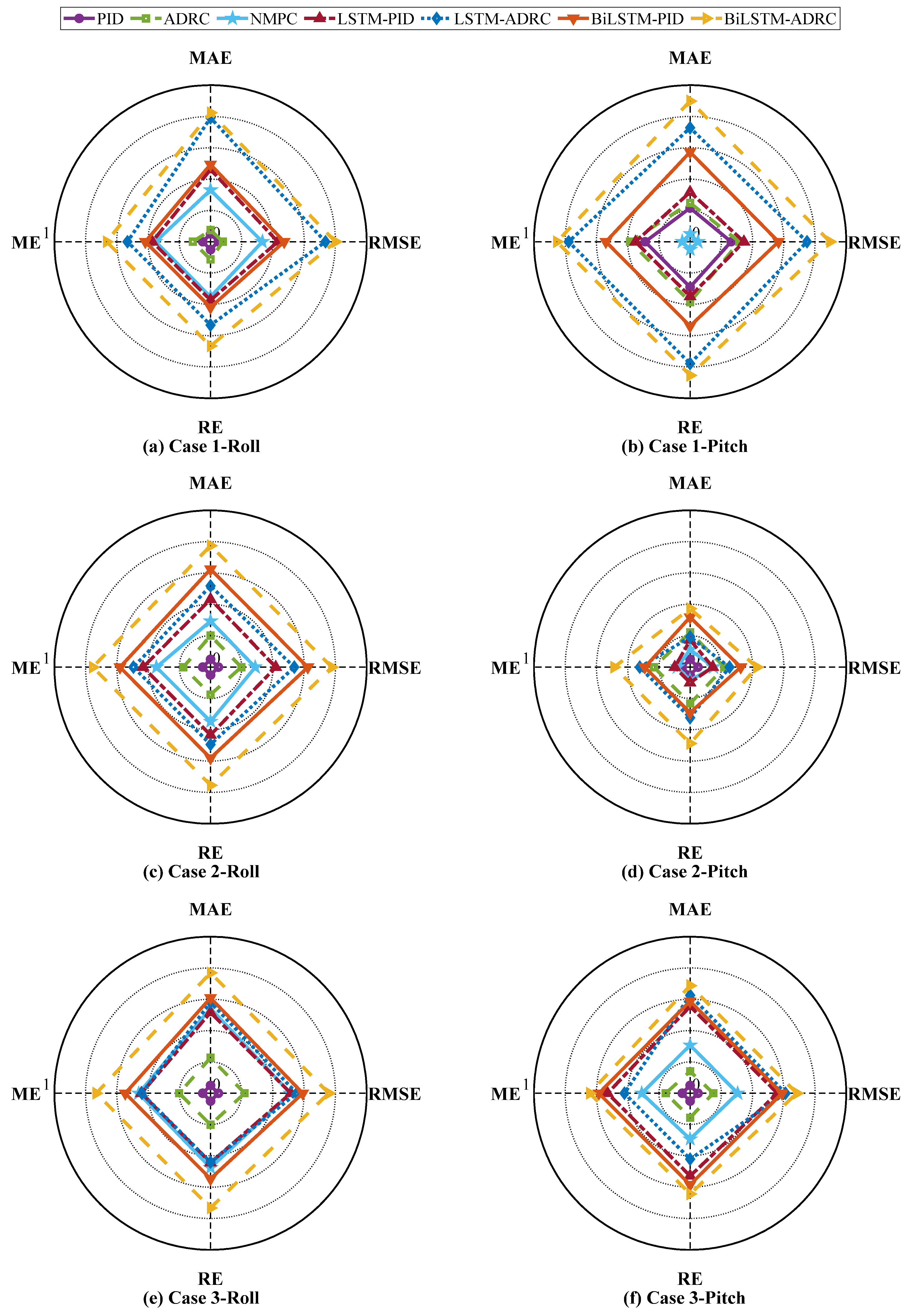
As illustrated in Figure 17, the error metrics are first normalized, and the normalized results are further transformed using the 1–normalized value scheme. After this transformation, larger metric values indicate a better control performance, thereby enabling a visualization in which outward expansion in the radar charts corresponds to performance improvement. The experimental results demonstrate that the traditional PID and ADRC methods exhibit relatively limited overall performance improvements across different operating conditions. The compensation performance of NMPC is improved compared with the former two control methods; however, it remains inferior to the control strategies based on deep learning prediction. In contrast, control strategies incorporating LSTM-based prediction show clear advantages over most evaluation metrics, as evidenced by the significantly enlarged radar chart coverage, indicating that the inclusion of predictive information effectively reduces system errors and enhances dynamic response performance. Further comparative analysis reveals that BiLSTM-based control strategies achieve higher normalized performance values across the majority of evaluation metrics. In particular, the BiLSTM–ADRC method consistently attains the best or second-best overall performance under different operating conditions and attitude channels, with a more balanced radar chart profile and the largest overall coverage area. These results further confirm that the integrated BiLSTM–ADRC strategy delivers a superior and more stable comprehensive performance in terms of compensation accuracy, peak suppression capability, and relative error regulation under complex sea state conditions.

5. Conclusions

This study introduces a wave compensation strategy for a Stewart platform that integrates deep learning prediction with disturbance rejection control, with the goal of enhancing the attitude stability of onboard equipment in complex sea conditions. This approach utilizes a BiLSTM model for the proactive prediction of the vessel’s attitude, effectively addressing the time delay issues inherent in the motion compensation process. It is combined with a cascaded ADRC controller to achieve robust wave compensation control in the presence of significant external disturbances. The simulation results indicate that the proposed method substantially outperforms comparative control strategies, including PID, ADRC, NMPC, LSTM-PID, LSTM-ADRC, and BiLSTM-PID, in compensating for roll and pitch angles. This improvement not only enhances the system’s disturbance rejection capability but also improves real-time response performance.

However, there is still room for further enhancement in the prediction accuracy of the vessel’s attitude, particularly under extreme sea conditions or in scenarios involving long time series forecasting. Moreover, the ADRC controller’s parameters depend on empirical tuning, which complicates the parameter adjustment process. Future research could explore the integration of attention mechanisms or other advanced neural network architectures to improve prediction accuracy while also implementing online adaptive or reinforcement learning methods to optimize control parameters and enhance the system’s wave disturbance compensation capability.

References

1. Zhou, Z.; Zhang, B.; Chang, J.; Dong, Q.; Wang, H. Dynamic response analysis of the vessel under the action of motion compensation equipment. Ocean Eng. 2025, 315, 119885. [Google Scholar] [CrossRef] [Scilit]
2. Qiu, W.; Wang, S.; Niu, A.; Fan, K.; Han, G.; Chen, H. Modeling and analysis of landing collision dynamics for an active helideck based on the Stewart platform. Ocean Eng. 2024, 297, 117107. [Google Scholar] [CrossRef] [Scilit]
3. Chen, W.; Wen, Y.; Tong, X.; Lin, C.; Li, J.; Wang, S.; Xie, W.; Mao, L.; Zhao, X.; Zhang, W.; et al. Dynamics modeling and modal space control strategy of ship-borne Stewart platform for wave compensation. J. Mech. Robot. 2023, 15, 041015. [Google Scholar] [CrossRef] [Scilit]
4. Kong, X. Composite Control for a Class of Strong Coupling/Strong Uncertainty/Strong Nonlinearity and Fast Time Varying Systems. J. Astronaut. 2019, 40, 1422. [Google Scholar]
5. Furqan, M.; Suhaib, M.; Ahmad, N. Studies on Stewart platform manipulator: A review. J. Mech. Sci. Technol. 2017, 31, 4459–4470. [Google Scholar] [CrossRef] [Scilit]
6. Russo, M.; Zhang, D.; Liu, X.J.; Xie, Z. A review of parallel kinematic machine tools: Design, modeling, and applications. Int. J. Mach. Tools Manuf. 2024, 196, 104118. [Google Scholar] [CrossRef] [Scilit]
7. Paccot, F.; Andreff, N.; Martinet, P. A review on the dynamic control of parallel kinematic machines: Theory and experiments. Int. J. Robot. Res. 2009, 28, 395–416. [Google Scholar] [CrossRef] [Scilit]
8. Jiang, M.; Rui, X.; Zhu, W.; Yang, F.; Zhang, J. Modeling and control of magnetorheological 6-DOF stewart platform based on multibody systems transfer matrix method. Smart Mater. Struct. 2020, 29, 035029. [Google Scholar] [CrossRef] [Scilit]
9. Ayas, M.S.; Sahin, E.; Altas, I.H. High order differential feedback controller design and implementation for a Stewart platform. J. Vib. Control 2020, 26, 976–988. [Google Scholar] [CrossRef] [Scilit]
10. Kim, Y.S.; Shi, H.; Dagalakis, N.; Marvel, J.; Cheok, G. Design of a six-DOF motion tracking system based on a Stewart platform and ball-and-socket joints. Mech. Mach. Theory 2019, 133, 84–94. [Google Scholar] [CrossRef] [Scilit]
11. He, Y.; Wang, H.; Tian, Y.; Zhou, X. Model-Free Based Nonsingular Fast Terminal Sliding Mode Control for Gough-Stewart Platform. In Proceedings of the 42nd Chinese Control Conference (CCC), Tianjin, China, 24–26 July 2023; IEEE: New York, NY, USA, 2023; pp. 2370–2375. [Google Scholar]
12. Safeena, M.K.; Jiji, K.S. Control of Stewart platform using adaptive smooth integral sliding mode algorithm. ISA Trans. 2025, 156, 99–108. [Google Scholar]
13. Cai, Y.; Zheng, S.; Liu, W.; Qu, Z.; Zhu, J.; Han, J. Sliding-mode control of ship-mounted Stewart platforms for wave compensation using velocity feedforward. Ocean Eng. 2021, 236, 109477. [Google Scholar] [CrossRef] [Scilit]
14. Wen, Y.; Li, W.; Zhou, S.; Gao, F.; Chen, W. Robust sliding mode control with adaptive gravity estimation of ship-borne Stewart platform for wave compensation. Appl. Ocean Res. 2024, 148, 104004. [Google Scholar] [CrossRef] [Scilit]
15. Chen, W.; Wang, S.; Li, J.; Lin, C.; Yang, Y.; Ren, A.; Li, W.; Zhao, X.; Zhang, W.; Guo, W.; et al. An ADRC-based triple-loop control strategy of ship-mounted Stewart platform for six-DOF wave compensation. Mech. Mach. Theory 2023, 184, 105289. [Google Scholar] [CrossRef] [Scilit]
16. Liu, J.; Chen, X. Adaptive control based on neural network and beetle antennae search algorithm for an active heave compensation system. Int. J. Control Autom. Syst. 2022, 20, 515–525. [Google Scholar] [CrossRef] [Scilit]
17. Qiang, H.; Wang, Y.; Wang, R.; Liu, K.; Kang, S.; Yang, J. Model predictive control considering load disturbance of ship-borne hydraulic parallel platform. IEEE Access 2024, 12, 197201–197216. [Google Scholar] [CrossRef] [Scilit]
18. Wang, L.; Jiang, J.; Wang, M. Research on MPC control of a 6 DOF Stewart platform. In Proceedings of the 2022 IEEE International Conference on Manipulation, Manufacturing and Measurement on the Nanoscale (3M-NANO), Tianjin, China, 8–12 August 2022; IEEE: New York, NY, USA, 2022; pp. 65–69. [Google Scholar]
19. Mochida, R.; Ishimura, K.; Akita, T.; Kon, T. High-Precision Pointing Control Using Stewart Platform with Adaptive Model Predictive Control. J. Spacecr. Rocket. 2025, 62, 1310–1327. [Google Scholar] [CrossRef] [Scilit]
20. Peled, D.; Iosti, S.; Bensalem, S. Control synthesis through deep learning. In From Reactive Systems to Cyber-Physical Systems: Essays Dedicated to Scott A. Smolka on the Occasion of His 65th Birthday; Springer International Publishing: Cham, Switzerland, 2019; pp. 242–255. [Google Scholar]
21. Li, D.; Wang, S.; Song, X.; Zheng, Z.; Tao, W.; Che, J. A BP-Neural-Network-Based PID Control Algorithm of Shipborne Stewart Platform for Wave Compensation. J. Mar. Sci. Eng. 2024, 12, 2160. [Google Scholar] [CrossRef] [Scilit]
22. Yin, L.; Yu, T.; Zhang, X.; Yang, B. Relaxed deep learning for real-time economic generation dispatch and control with unified time scale. Energy 2018, 149, 11–23. [Google Scholar] [CrossRef] [Scilit]
23. Wang, Z.; Xiang, X.; Duan, Y.; Yang, S. Adversarial deep reinforcement learning based robust depth tracking control for underactuated autonomous underwater vehicle. Eng. Appl. Artif. Intell. 2024, 130, 107728. [Google Scholar]
24. Belhaj Salah, L.; Fourati, F. A greenhouse modeling and control using deep neural networks. Appl. Artif. Intell. 2021, 35, 1905–1929. [Google Scholar] [CrossRef] [Scilit]
25. Chen, X.; Jiao, Y.; Yuan, X.; Meng, Z.; Zhang, L.; Liu, X. An online dual-loop AMPC strategy for wave compensation of an electro-hydraulic servo Stewart platform. Control Eng. Pract. 2025, 165, 106540. [Google Scholar] [CrossRef] [Scilit]
26. Chang, S.; Cao, J.; Pang, J.; Zhou, F.; Chen, W. Compensation control strategy for photoelectric stabilized platform based on disturbance observation. Aerosp. Sci. Technol. 2024, 145, 108909. [Google Scholar] [CrossRef] [Scilit]
27. Qu, X.; Li, Z.; Chen, Q.; Peng, C.; Wang, Q. Research on improved active disturbance rejection control strategy for hydraulic-driven Stewart stabilization platform. Ind. Robot. Int. J. Robot. Res. Appl. 2024, 51, 881–889. [Google Scholar] [CrossRef] [Scilit]
28. Yin, R.; Xie, W.; Wen, Y.; Zhang, C.; Chen, W.; Zhang, W. Robust wave compensation controller design for an active hexapod platform with time-varying input delays. Ocean Eng. 2023, 274, 114084. [Google Scholar] [CrossRef] [Scilit]
29. Cai, Y.; Zheng, S.; Liu, W.; Qu, Z.; Han, J. Model analysis and modified control method of ship-mounted Stewart platforms for wave compensation. IEEE Access 2020, 9, 4505–4517. [Google Scholar] [CrossRef] [Scilit]
30. Zhou, Y.; She, J.; Wang, F.; Iwasaki, M. Disturbance rejection for stewart platform based on integration of equivalent-input-disturbance and sliding-mode control methods. IEEE/ASME Trans. Mechatron. 2023, 28, 2364–2374. [Google Scholar] [CrossRef] [Scilit]
31. Huang, Y.; Xue, W. Active disturbance rejection control: Methodology and theoretical analysis. ISA Trans. 2014, 53, 963–976. [Google Scholar] [CrossRef] [Scilit]
32. Zhang, Y.; Chen, Z.; Zhang, X.; Sun, Q.; Sun, M. A novel control scheme for quadrotor UAV based upon active disturbance rejection control. Aerosp. Sci. Technol. 2018, 79, 601–609. [Google Scholar] [CrossRef] [Scilit]
33. Xu, L.X.; Ma, H.J.; Guo, D.; Xie, A.H.; Song, D.L. Backstepping sliding-mode and cascade active disturbance rejection control for a quadrotor UAV. IEEE/ASME Trans. Mechatron. 2020, 25, 2743–2753. [Google Scholar] [CrossRef] [Scilit]
34. Qu, L.; Qiao, W.; Qu, L. Active-disturbance-rejection-based sliding-mode current control for permanent-magnet synchronous motors. IEEE Trans. Power Electron. 2020, 36, 751–760. [Google Scholar] [CrossRef] [Scilit]
35. Bilal, H.; Yin, B.; Aslam, M.S.; Anjum, Z.; Rohra, A.; Wang, Y. A practical study of active disturbance rejection control for rotary flexible joint robot manipulator. Soft Comput. 2023, 27, 4987–5001. [Google Scholar] [CrossRef] [Scilit]
36. Sun, Q.; Tang, Z.; Gao, J.; Zhang, G. Short-term ship motion attitude prediction based on LSTM and GPR. Appl. Ocean Res. 2022, 118, 102927. [Google Scholar] [CrossRef] [Scilit]
37. Wang, Y.; Wang, H.; Zhou, B.; Fu, H. Multi-dimensional prediction method based on Bi-LSTMC for ship roll. Ocean Eng. 2021, 242, 110106. [Google Scholar] [CrossRef] [Scilit]
38. Wang, Y.; Dou, Y.; Yang, Z.; Fu, H. Ship pitch prediction method based on LSTMC and multi-head attention. Ocean Eng. 2024, 309, 118236. [Google Scholar] [CrossRef] [Scilit]
39. Angeles, J. (Ed.) Fundamentals of Robotic Mechanical Systems: Theory, Methods, and Algorithms; Springer: New York, NY, USA, 2003. [Google Scholar]
40. Wang, W.; Ning, Y.; Zhang, Y.; Xu, P.; Li, B. Linear active disturbance rejection control with linear quadratic regulator for Stewart platform in active wave compensation system. Appl. Ocean Res. 2025, 156, 104469. [Google Scholar] [CrossRef] [Scilit]
41. Kane, T.R.; Levinson, D.A. The use of Kane’s dynamical equations in robotics. Int. J. Robot. Res. 1983, 2, 3–21. [Google Scholar] [CrossRef] [Scilit]
42. Domala, V.; Kim, T.W. Application of Empirical Mode Decomposition and Hodrick Prescot filter for the prediction single step and multistep significant wave height with LSTM. Ocean Eng. 2023, 285, 115229. [Google Scholar] [CrossRef] [Scilit]
43. Schuster, M.; Paliwal, K.K. Bidirectional recurrent neural networks. IEEE Trans. Signal Process. 1997, 45, 2673–2681. [Google Scholar] [CrossRef] [Scilit]
44. Wan, A.; Peng, S.; Khalil, A.B.; Ji, Y.; Ma, S.; Yao, F.; Ao, L. A novel hybrid BWO-BiLSTM-ATT framework for accurate offshore wind power prediction. Ocean Eng. 2024, 312, 119227. [Google Scholar] [CrossRef] [Scilit]
45. Chen, Y.J.; Huang, H.; Chen, Z.S. AVOA-optimized CNN-BILSTM-SENet framework for hydrodynamic performance prediction of bionic pectoral fins. Ocean Eng. 2025, 327, 121002. [Google Scholar] [CrossRef] [Scilit]
46. Han, J. From PID to active disturbance rejection control. IEEE Trans. Ind. Electron. 2009, 56, 900–906. [Google Scholar] [CrossRef] [Scilit]
Figure 1. Ship-mounted Stewart platform for wave compensation.
Actuators 15 00140 g001
Figure 2. The proposed integrated control framework.
Actuators 15 00140 g002
Figure 3. Deep learning-based forecasting module.
Actuators 15 00140 g003
Figure 4. Wave energy under three sea states. (a) Case 1; (b) Case 2; (c) Case 3.
Actuators 15 00140 g004
Figure 5. Roll and pitch motions. (a) Case 1; (b) Case 2; (c) Case 3.
Actuators 15 00140 g005
Figure 6. Prediction time comparison.
Actuators 15 00140 g006
Figure 7. Validation loss curve.
Actuators 15 00140 g007
Figure 8. Comparison of predicted results.
Actuators 15 00140 g008
Figure 9. Box plot of errors for predicted results.
Actuators 15 00140 g009
Figure 10. Bar chart of error statistics.
Actuators 15 00140 g010
Figure 11. Compensation performance in Case 1.
Actuators 15 00140 g011
Figure 12. Compensation performance in Case 2.
Actuators 15 00140 g012
Figure 13. Compensation performance in Case 3.
Actuators 15 00140 g013
Figure 14. Model comparison in Case 1.
Actuators 15 00140 g014
Figure 15. Model comparison in Case 2.
Actuators 15 00140 g015
Figure 16. Model comparison in Case 3.
Actuators 15 00140 g016
Figure 17. Radar chart of error metrics.
Actuators 15 00140 g017