Intelligent Soft Sensors for Inferential Monitoring of Hydrodesulfurization Process Analyzers

Abstract

This work presents the development of soft sensor models for monitoring the operation of online process analyzers used to measure the sulfur content in the product of the refinery hydrodesulfurization process. Since sulfur content often fluctuates over time, soft sensor models must account for these frequency fluctuations. We have therefore developed dynamic data-driven models based on linear and nonlinear system identification techniques (finite impulse response—FIR, autoregressive with exogenous inputs—ARX, output error—OE, nonlinear ARX—NARX, Hammerstein–Wiener—HW) and machine learning techniques, including models based on long short-term memory (LSTM) and gated recurrent unit (GRU) networks, as well as artificial neural networks (ANNs). The core steps in model development included the selection and preprocessing of continuously measured plant process data, collected from a full-scale industrial hydrodesulfurization unit under normal operating conditions. The developed soft sensor models are intended to support or replace process analyzers during maintenance periods or equipment failures. Moreover, these models enable the application of inferential control strategies, where unmeasured process variables—such as sulfur content—can be estimated in real time and used as feedback for advanced process control.

1. Introduction

In industrial processes and plants, it is often difficult to measure most of the key process variables and product properties continuously and reliably. These quantities are typically monitored by laboratory analysis, which are infrequent and time-consuming. On the other hand, the use and maintenance of online process analyzers can be extremely demanding and expensive. For these reasons, soft sensors are introduced into the application to monitor the most important process variables. Thanks to soft sensors based on easily measurable secondary variables such as temperature, pressure, and flow, the behavior of difficult-to-measure variables is predicted by determining their mathematical functional relationships. The development of soft sensors in chemical engineering requires knowledge from various technical fields, and the synergy of scientific research and the experience of technologists and plant operators is also important.

In modern oil refineries, it is necessary to remove sulfur from the final product when producing fuels. Fuels often contain smaller or larger quantities of sulfur, which can have a negative impact on the environment. When fuels (diesel or gasoline) are burned, the sulfur in the fuel reacts with oxygen and forms sulfur dioxide (SO₂), which is an air pollutant and contributes to acid rain, smog, and various respiratory diseases.

Hydrodesulfurization (HDS) is a petroleum refining process for removing sulfur from fuels. In our case, we are talking about diesel fuel. The permissible sulfur content in diesel fuel is 10 mg/kg according to the current European Directive 2016/802/EU [1]. In hydrodesulfurization plants, the sulfur content is determined by laboratory analyses and online process analyzers. Process analyzers are expensive, and if they are not regularly maintained, they often fail.

Due to the irregularity of laboratory analyses and possible frequent failures of process analyzers, situations often arise where key process variables are measured irregularly, affecting product quality or resulting in products not meeting the required specifications. An alternative to performing irregular laboratory analysis is the use of soft sensor models that monitor the operation of process analyzers and serve as a backup in the event of regular maintenance or failure.

A soft sensor (virtual soft sensor/software sensor/soft analyzer) is defined as a mathematical model, analytical or empirical, that is used to estimate important non-measurable process variables. Soft sensors can be roughly divided into two classes: data-driven and first-principle sensors. Since first-principle models are usually created for plant design and therefore focus on describing steady-state process behavior, they are difficult to develop. In contrast, data-driven soft sensors are based on measured data and provide a more realistic description of the real process dynamics of complicated industrial processes [2]. The selection and preparation of continuously measured process data from the plant were essential elements in the construction of a data-driven model. The selection of historical data from the plant database, the detection of outliers, data filtering, the selection of the model structure and regressors, and model estimation and validation are typical steps in the development process [3].

Once the models have been developed and validated, an attempt is made to select the optimal models in terms of accuracy and structure for use in a real plant. With the support or replacement of process analyzers, such models can also be used for inferential control. Inferential control is a control strategy in which the controlled variable is not measured directly but is estimated using secondary inference variables. The estimated value is then used in a feedback loop to keep the controlled variable at the desired setpoint [4].

System identification is the process of creating mathematical models of dynamic systems based on measured input–output data. It is often used in control engineering, signal processing, and machine learning, especially when first-principles models are too complex or unknown. The Swedish scientist L. Ljung is one of the founders of modern system identification. He developed and popularized dynamic polynomial model structures, estimation methods and robust techniques for validating models. Popular model structures that are also used in this work are finite impulse response (FIR), autoregressive with exogenous inputs (ARX), output error (OE), nonlinear ARX (NARX), and Hammerstein–Wiener (HW) [5].

Artificial neural networks (ANNs) were originally created as mathematical models that can process data in a similar way to a biological brain. The basic structure of an ANN consists of a network of tiny nodes connected by weighted links. The biological paradigm uses nodes to represent neurons and connection weights to indicate the strength of synapses between neurons. By giving an input to some or all nodes, one can activate the entire network; the weighted connections then ensure that this activation is distributed throughout the network [6]. If they are well trained and properly validated, mathematical models based on such structures can easily be applied as soft sensors in plants if the process dynamics are not too pronounced. For plants, where the dynamics are more pronounced, models based on dynamic neural network structures, such as the very popular long short-term memory (LSTM) and the gated recurrent unit (GRU), may prove more successful. The LSTM enables effective modeling and learning from data sequences. It works according to the gate principle—it controls the importance of the data in different time intervals so that it ignores the irrelevant ones and stores the important information of the input data in the past time intervals, thus preventing the problem of the vanishing gradient, i.e., limiting the depth and complexity of the networks [6,7]. On the other hand, GRU networks are designed to increase the speed of LSTM networks when large amounts of data are involved. The core principle of a GRU is to clarify the inner composition of the LSTM in order to minimize the network complexity [8].

Numerous papers have been published in recent years on the topic of soft sensor models based on dynamic polynomial models and models of machine learning and inferential control. The papers range from basic research to application and cover all areas of technology. Here we will list some that relate to chemical engineering and related fields.

In a recently published paper [9], the authors presented the development of a model based on LSTM and convolutional neural networks (CNNs) intended for the prediction of sulfur dioxide (SO₂) concentration in the flue gas of coal-fired power plants. The validation of the model showed its very good accuracy. LSTM networks were used for the inferential control of a distillation column in a petroleum refinery process for the separation of an azeotropic mixture of toluene (TL) and 2-methoxyethanol (2-ME). The simulation results showed that the model-based control has a lower deviation and fewer oscillations compared to the traditional closed-loop control [10]. Researchers have also successfully used LSTM networks in the development of inferential flow controls in hydraulic systems [11]. By combining LSTM and CNN networks, the authors presented a successfully developed model for detecting faults in the air handling unit (AHU), an essential component of heating, ventilation, and air conditioning (HVAC) systems [12]. Various machine learning techniques were not omitted in the recently published work, where they were successfully applied to the processes of carbon capture [13].

The development of artificial intelligence (AI) is having a major impact on the automotive industry. Artificial intelligence is mainly present in quality control and maintenance. In [14], models based on different ANN structures for fault detection, process automation and predictive maintenance are compared.

A recently published study [15] compares different machine learning-based models, including static and dynamic neural network structures, for predicting process variables for two nonlinear chemical engineering systems: a plug-flow reactor for vapor phase cracking of acetone and a pilot-plant for carbon dioxide capture. The results of the model validation proved to be satisfactory. A valuable work by Indian scientists [16] involving the use of the system identification technique (NARX) in combination with a particle swarm optimization (PSO) algorithm provides an innovative approach for modeling the dynamics of cryogenic vessels. Another interesting piece of work involving the NARX technique of system identification is the development and application of a model for liquid level systems in industrial processes [17].

Pressure swing adsorption (PSA) is a process that enables the production of high purity products, such as high purity hydrogen. However, the inherent trade-offs between purity, productivity and cycle work are sometimes difficult to realize. In the paper [18], the authors presented an efficient model based on ANNs to optimize and balance the performance of the PSA process.

The manufacture of metal products is also an area that has been enriched by the development of artificial intelligence methods. For example, in paper [19], the authors presented a proposal for the application of ANNs to develop models for quality control in the manufacture of drive shafts. The model would be successfully used to identify critical quality problems such as cracks, scratches, and dimensional deviations.

The production of lithium-ion batteries is very advanced today. However, the behavior of the batteries during their life cycle has not yet been sufficiently investigated. In one study [20], researchers used the recently very popular system identification technique NARX to predict the behavior of the battery. The proposed model proved to be very accurate for predicting the characteristics of such batteries, such as state of charge (SoC), voltage, and current under dynamic conditions. Researchers at the Karlsruhe Institute of Technology in Germany have developed a NARX model that predicts useful relationships between the torque of an electric vehicle with lithium-ion batteries and characteristics such as the speed of the electric motor and the vehicle [21].

For modeling strongly nonlinear systems, it is sometimes useful to apply the Hammerstein–Wiener technique of system identification. In one paper [22], such a method was successfully used to design a control system for a propeller pendulum. The Hammerstein–Weiner in combination with other system identification techniques, such as ARX, has been successfully used to create a dynamic model of the electrolysis process and to estimate the system variables [23].

An interesting paper has been published [24] related to the development of linear and nonlinear soft sensor models to predict the research octane number (RON), which is an important quality parameter for gasoline in refinery production. Among the different models compared, models based on ANNs and support vector machines regression (SVM) stand out. Also, from the field of refinery production comes an interesting article [25], in which several machine learning methods are combined to develop a soft sensor model for predicting a frequently required parameter such as the flash point temperature of automotive fuels. Such processes can also release large quantities of NO_x compounds, the concentrations of which are often difficult to monitor. In the paper [26], GRU neural networks were used to create a precise model for predicting NO_x emission concentrations.

Regarding the process of hydrodesulfurization in refineries, there are not many works dealing with the development of software sensor models to predict the sulfur content in the product. Only a few relevant works from the past can be singled out. A group of Iranian researchers has developed robust models based on the machine learning technique support vector machine regression to predict the sulfur content in the HDS process [27,28]. Also of interest are articles describing the development and application of software sensors based on ANNs for predicting sulfur content [29,30].

The hydrodesulphurization process in a refinery operation is highly nonlinear and time-dependent, with the controlled variable (sulfur content in the product) often fluctuating over time. A review of the available literature revealed a lack of studies focusing on the development of predictive models that explicitly account for these temporal fluctuations. Our paper therefore presents the comprehensive and systematic development of polynomial dynamic data-driven models based on linear and nonlinear system identification techniques (FIR, ARX, OE, NARX, HW) and machine learning techniques, including models based on LSTM and GRU networks, as well as ANNs, for the estimation of sulfur content. A comprehensive comparison of the model results is presented. The aim is to identify optimal model structures as soft sensors to support or replace process analyzers for measuring sulfur content during their maintenance periods or in case of failures. This methodological framework contributes to soft sensor development practice and supports real-world applications such as analyzer backup and inferential control.

2. Materials and Methods

2.1. Process Description

Hydrodesulfurization (HDS) is a process in which petroleum products and intermediates are treated with hydrogen in the presence of a catalyst to remove sulfur compounds. Hydrodesulfurization is a form of mild hydrocracking in which nitrogen and oxygen compounds, along with sulfur compounds, are removed, hydrocarbon compounds containing double bonds are hydrogenated, and the metal content is reduced. Hydrodesulfurization increases the chemical stability of gasoline and the cetane number and stability of diesel fuels, so it can be said that this process generally improves the environmental and application properties of petroleum fuels [31].

Figure 1 shows a general process diagram of the HDS process. Fresh feedstock (usually naphtha or diesel fuel from an atmospheric distillation unit) is combined with hydrogen, heated, and enters the HSD reactor where hydrodesulfurization and saturation reactions of unsaturated compounds such as olefins and aromatics take place. The hydrodesulfurized product is then cooled and fed into a high-pressure separator where the desired product is separated at the bottom and gases, mainly hydrogen, are separated at the top. The separated product is fed into a stripper column where light hydrocarbons are additionally separated at the top of the column and sent for purification in the form of “sour” hydrocarbon gas via a reflux tank. The product at the bottom of the stripping column is cooled and stored as a finished hydrodesulfurized product [31].

2.2. Theoretical Background

2.2.1. System Identification Techniques

The techniques of system identification are well explained by Ljung [5]. Structures of polynomial dynamic linear and nonlinear models are elaborated.

The simplest polynomial dynamic linear model is FIR (finite impulse response), whose predictor is represented by the following equation:

$$\widehat{y}(t)=\mathbf{B}(q)u(t-nk),$$

(1)

where $\mathbf{B}(q)={\mathbf{B}}_1+{\mathbf{B}}_2{q}^{-1}+\mathrm{\dots }+{\mathbf{B}}_{nb}{q}^{-nb+1}$ is a polynomial matrix by q⁻¹, nb is the number of past process input samples, and nk is the input time delay expressed as the number of samples.

ARX (autoregressive with exogenous inputs) is a linear model that also takes into account the presence of noise. The predictor of the model is:

$$\widehat{y}(t)=\left[1-\mathbf{A}(q)\right]y(t)+\mathbf{B}(q)u(t-nk),$$

(2)

where $\mathbf{A}(q)=1+{\mathbf{A}}_1{q}^{-1}+{\mathbf{A}}_2{q}^{-2}+\mathrm{\dots }+{\mathbf{A}}_{na}{q}^{-na}$ is a polynomial matrix by q⁻¹, na is the number of past process output samples.

OE (output error) is a linear model whose predictor is:

$$\widehat{y}(t)=\left[1-\mathbf{F}(q)\right]\widehat{y}(t)+\mathbf{B}(q)u(t-nk),$$

(3)

where $\mathbf{F}(q)=1+{\mathbf{F}}_1{q}^{-1}+{\mathbf{F}}_2{q}^{-2}+\mathrm{\dots }+{\mathbf{F}}_{nf}{q}^{-nf}$ is polynomial matrix by q⁻¹, nf is the number of past output samples predicted by the model.

While the structure of linear models is completely determined by the selected regressors, the structure of nonlinear models also depends on the properties of a nonlinear function. NARX is a nonlinear version of the ARX model. The predictor has a linear regression form with an additional nonlinear part:

$$\widehat{y}(t)=f_n\left[y(t-1),\mathrm{\dots },y(t-na),u(t-nk),\mathrm{\dots },u(t-nk)-nb+1\right],$$

(4)

where f_n is a nonlinear function that represents the number of nonlinear units, which can be different types of network structures, such as wavelet, sigmoid, piecewise-linear, and others. The most complex nonlinear dynamic model is the HW (Hammerstein–Wiener) model, which is characterized by a block structure consisting of three different functions: w(t) = f(u(t)) performs a nonlinear transformation of the input data u(t); x(t) = (B/F)w(t) is a linear transfer function, where B and F are polynomials associated with an OE model; ŷ(t) = h(x(t)) is a nonlinear function that maps the output of the linear block to the final model output. Similarly to the NARX model, the nonlinear functions in this structure can be expressed by a series of nonlinear units.

2.2.2. Artificial Neural Networks (ANNs)

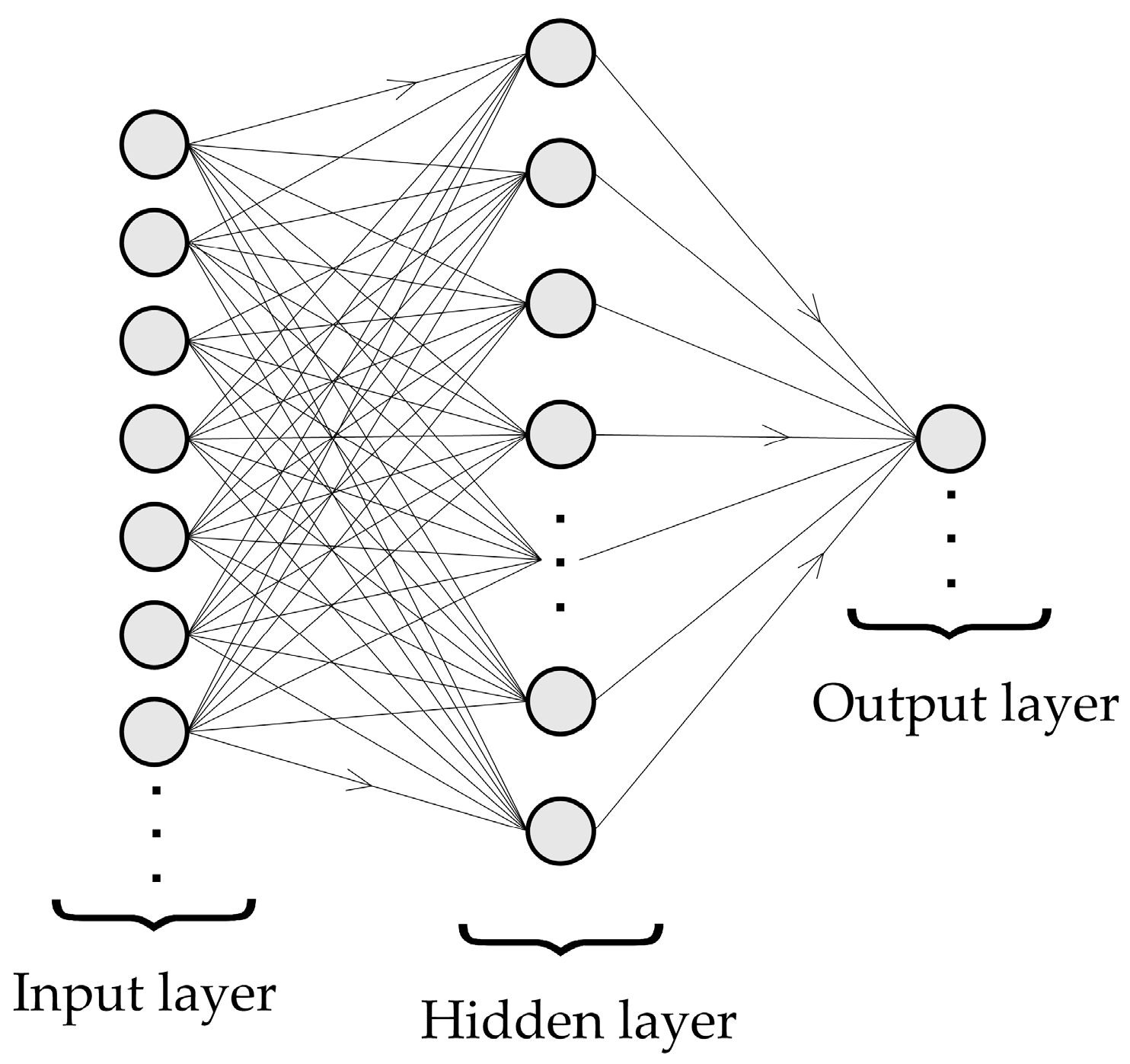
Figure 2 illustrates the architecture of a multilayer perceptron (MLP), which is a category of ANNs. The network consists of sequentially connected layers of units, with signals propagating from the input layer through one or more hidden layers to the output layer. This propagation is called the feedforward phase. Since the output of an MLP is determined solely by the current input—without taking into account information from previous or future inputs—MLPs are generally less suitable for dynamic tasks such as time series regression. Each specific configuration of weights within an MLP defines a particular input–output mapping. By changing these weights, the MLP can approximate a wide range of functions [6].

2.2.3. Long Short-Term Memory Networks (LSTM)

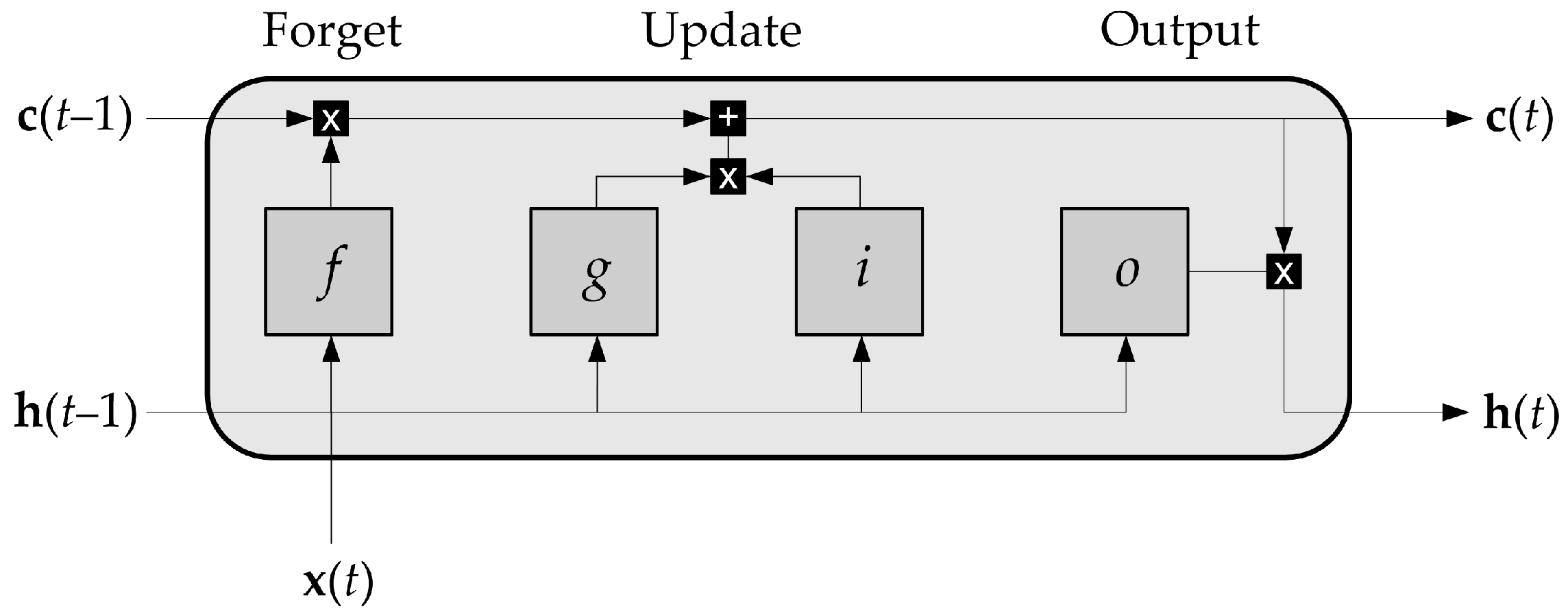
LSTM networks often prove to be particularly effective for processes with a more pronounced dynamic behavior. These networks work on the basis of the gating mechanism, which regulates the relevance of information over different time steps, filtering out unimportant data while retaining important input features. The LSTM architecture consists of recurrently connected sub-networks called memory units. Each unit contains a memory cell and nonlinear gates that enable selective storage of relevant current information and discarding of obsolete or irrelevant data [7]. A standard structure of an LSTM unit is shown in Figure 3.

At time t, the LSTM unit consists of two main components: the output state h(t), which represents the current output, and the cell state c(t), which contains information from previous time steps, in particular from h(t–1) and c(t–1). At each time step, the cell state c(t) is updated by selectively adding or removing information using gates. The most recent input at time t is referred to as x(t).

The LSTM unit comprises the following key elements: the input gate i, which updates the input by integrating the current input with the previous output and cell states; the forget gate f, which determines which information from the previous cell state should be discarded; the output gate o, which is responsible for computing the current output; and the cell input g, which refines the input by combining the current input and the previous output state. The parameters learned during training consist of the input weighting matrix W, the recurrent weighting matrix R, and the bias vector b. These are organized in the following matrix representations:

$$\mathbf{W}={\left[\begin{array}{cccc}{W}_i& W_f& W_g& W_o\end{array}\right]}^{\mathsf{T}};$$

(5)

$$\mathbf{R}={\left[\begin{array}{cccc}{R}_i& R_f& R_g& R_o\end{array}\right]}^{\mathsf{T}};$$

(6)

$$\mathbf{b}={\left[\begin{array}{cccc}{b}_i& b_f& b_g& b_o\end{array}\right]}^{\mathsf{T}},$$

(7)

where i, f, g, and o denote the input gate, the forgetting gate, the cell input, and the output gate, respectively.

In the following, the states of the individual components within the LSTM unit at time t, f(t), g(t), i(t), and o(t), are calculated, whereupon the cell state, c(t), and the output state, h(t), are finally calculated as follows:

$$\mathbf{c}(t)=f(t)\odot \mathbf{c}(t–1)+i(t)\odot g(t);$$

(8)

$$\mathbf{h}(t)=o(t)\odot {\sigma }_c(\mathbf{c}(t)),$$

(9)

where σ_c denotes the activation function and ⊙ is the Hadamard product—the pointwise multiplication of two vectors [7,33].

2.2.4. Gated Recurrent Unit Networks (GRU)

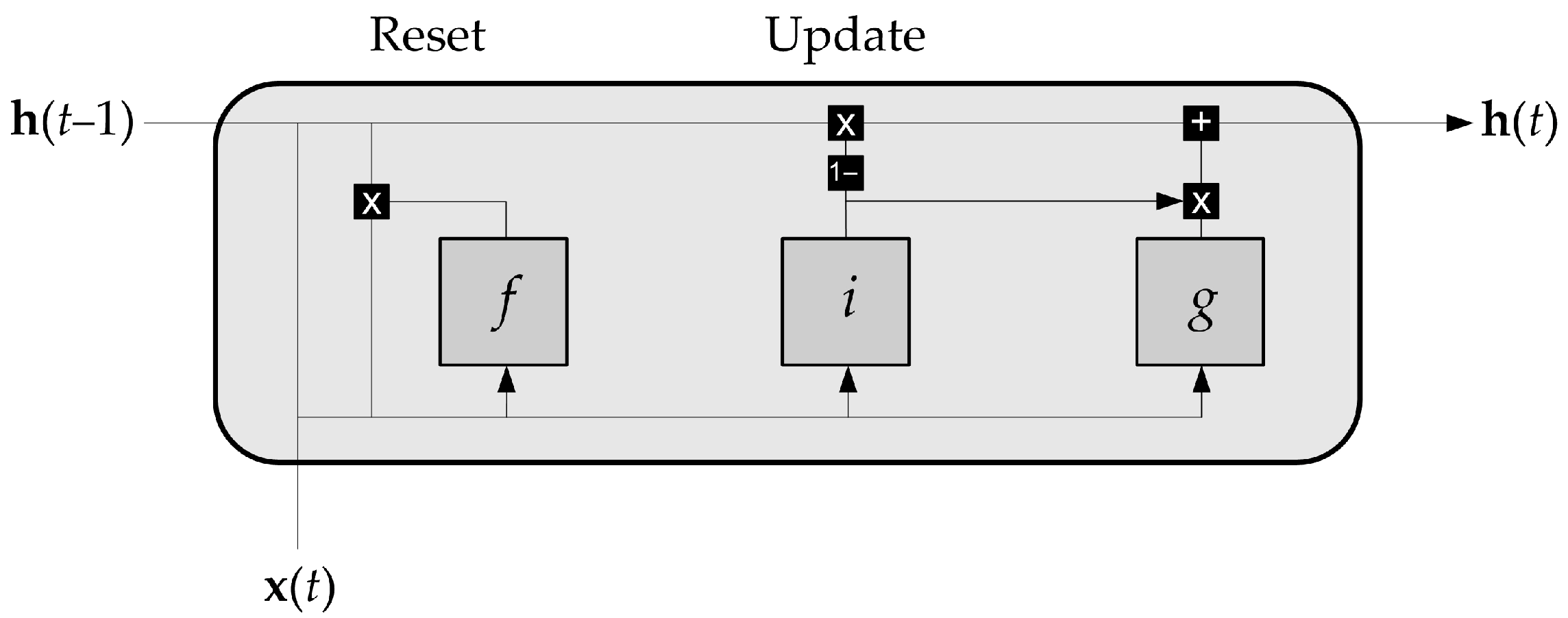
The basic concept of the GRU networks is to simplify the internal structure of the LSTM unit, thereby reducing the computational complexity of the network and improving the overall performance of the model. In contrast to the LSTM, the GRU has only two gating mechanisms: the update gate and the reset gate. The update gate controls the flow of information over time steps, while the reset gate controls the extent to which past information is retained or discarded [8]. A standard structure of a GRU is shown in Figure 4.

2.3. Model Development

The plant for hydrodesulfurization of diesel fuel is a complex industrial plant characterized by pronounced process dynamics and nonlinearity. The final product of the process is hydrodesulfurized diesel fuel with a permissible sulfur content of 10 mg/kg, in accordance with the current European Directive 2016/802/EU [1].

The data used for the model development was taken from the plant database, in which all measured variables are continuously stored. Several periods of plant operation in 2021 and 2022 were considered. An effort was made to identify a data set with emphasized process dynamics that lasts over a continuous period of at least ten days. Due to certain downtimes in plant operation and occasional malfunctions of the online process analyzer, it was challenging to select the relevant period. Ultimately, a period of 11 days in October 2022 was selected as the most appropriate for model development.

Preprocessing of the data included detection and removal of unexplained extreme values (outliers), data filtering, and eliminations of linear trends. A comprehensive feature analysis was performed that included the calculation of Pearson correlation coefficients to assess the relationships between input variables and an output variable, as well as descriptive statistics. The appropriate sampling time was also determined. Additionally, the output variable measured by the online process analyzer was compared with laboratory analysis results, which were conducted approximately four times per day, to assess measurement reliability. Since dynamic models are developed in the work, time delays for the input variables were also defined.

Based on the process analysis and consultations with technologists and plant operators, twenty variables were initially selected as potentially influential on the output variable (

Table 1. Potentially influential input variables.

Variable	Tag	Unit
V-001 vessel inlet temperature	TI-0201	°C
P-001 pump discharge feed flow	FC-0201	kg/h
total hydrogen flow	FI-0202N	m3/h
E-001A heat exchanger inlet temperature	TI-0202	°C
C-001 column hydrocarbons inlet temperature	TC-0701	°C
R-001 reactor feed inlet temperature	TC-0443	°C
R-001 reactor temperature	TC-0446	°C
R-001 reactor quench gas flow	FC-0401	kg/h
R-002 reactor quench gas flow	FC-0451	kg/h
R-002 reactor inlet temperature	TC-0493	°C
R-002 reactor outlet temperature	TI-0495	°C
V-003 LP separator hydrocarbons outlet flow	FC-0502	kg/h
C-001 column hydrocarbons inlet temperature	TI-0701.1	°C
C-001 column bottom outlet temperature	TI-0702	°C
C-001 column reflux flow	FC-0702	kg/h
V-006 vessel gas outlet flow	FI-0703	kg/h
“wild” naphtha to storage flow	FI-0704	kg/h
gas oil to storage flow	FC-1104	kg/h
E-004C heat exchanger inlet temperature	TI-0807	°C
gas oil to storage temperature	TI-1104	°C

).

Empirically, the optimum number of influencing variables is between six and eight. A larger number of input variables can lead to unnecessary complexity of the model, while with a smaller number of inputs it is likely that the model will not be able to describe the comprehensive process dynamics of complex industrial plants. An important fact is that the amount of sulfur at the input of the plant directly affects the amount of sulfur at the output of the plant, i.e., in the product. If the analysis determines that the raw material entering the process contains significantly more sulfur than the current value according to which the reactor inlet temperature is set, the reactor inlet temperature should be lowered, as desulfurization reactions are exothermic and a “temperature runaway” can occur.

Table 2. Pearson correlation coefficients between potentially influential input variables and the output variable.

Variable Tag	P. Corr. * with AI-0151	Mutual Score
TI-0201	−0.01	1.40
FC-0201	−0.24	0.43
FI-0202N	0.24	1.60
TI-0202	0.29	1.10
TC-0701	−0.35	0.54
TC-0443	−0.38	0.92
TC-0446	−0.44	1.90
FC-0401	0.17	1.50
FC-0451	−0.15	1.10
TC-0493	−0.59	1.50
TI-0495	−0.51	1.20
FC-0502	−0.23	1.30
TI-0701.1	−0.35	0.54
TI-0702	−0.47	0.73
FC-0702	−0.38	0.79
FI-0703	0.17	1.30
FI-0704	−0.27	1.50
FC-1104	−0.24	0.59
TI-0807	−0.47	0.56
TI-1104	−0.04	1.10

* Pearson correlation coefficients.

shows Pearson correlation coefficients between potentially influential input variables and the output variable.

Based on the Pearson correlation coefficients presented between potential input variables and the target output variable, several variables showed moderate to strong correlation with sulfur content in the product (e.g., TC-0493, TI-0495, TC-0446, TI-0702, TI-0807).

However, to avoid redundancy and potential multicollinearity within the model, an additional analysis of the Pearson correlations between the input variables was performed. The results are shown in Figure 5 (Pearson correlation matrix).

It was found that certain input variables were strongly correlated with each other (>0.9), especially for the temperature measurements associated with the reactor and stripping column sections. Consequently, some variables were excluded from further modeling even though they had a reasonable correlation with the target. Examples of this are as follows: TI-0702, which is strongly correlated with TI-0495 (≈0.95), TI-0807, which is strongly correlated with TC-0446 (≈0.91), and FI-0202N, which has a correlation with several flow-related variables.

The final selection of six influential input variables was based on a multi-criteria evaluation that included their correlation with the output variable, a mutual correlation, the coverage of different process sections (reactor and stripper column), and expert knowledge regarding process relevance.

Table 3. Influential input variables together with an output variable for the development of models to estimate the sulfur content in the product of the HDS process.

Variable	Tag	Unit
R-001 reactor feed inlet temperature	TC-0443	°C
C-001 column hydrocarbons inlet temperature	TC-0701	°C
R-001 reactor quench gas flow	FC-0401	kg/h
R-001 reactor temperature	TC-0446	°C
R-002 reactor inlet temperature	TC-0493	°C
R-002 reactor outlet temperature	TI-0495	°C
HDS diesel product sulfur content	AI-0151	mg/kg

shows the six selected influencing variables (plus one output variable) that were taken into account in the further steps of model development.

The HDS process under investigation is divided into four technological sections: reactor section, stripping section, amine gas treatment section and acid-water stripping section. Figure 6 shows the process flow diagram of the reactor section and the stripper section, which were the focus of the investigations carried out in this paper. All influential input variables and the output variable are marked in the figures.

Table 4. Descriptive statistics for the inputs and output.

Variable	Samples	Mean	Median	Min	Max	Variance	Std. Dev.
TC-0443	8900	331.9	331.4	323.3	341.1	8.090	2.884
TC-0701	8900	259.0	259.0	254.0	260.8	0.500	0.710
FC-0401	8900	1114	1107	845.1	1319	9053	95.15
TC-0446	8900	337.4	336.7	332.0	347.0	11.61	3.407
TC-0493	8900	332.2	332.3	327.2	340.0	6.690	2.587
TI-0495	8900	336.8	335.8	331.7	346.1	14.16	3.762
AI-0151	8900	9.860	10.05	4.400	16.18	3.730	1.931

shows descriptive statistics for the selected 6 input variables and the output variable with a sampling period of one minute. The maximum, minimum, mean, median, variance, and standard deviation are calculated. It can be observed that most temperatures are stable and controlled, with only minor deviations. The flow rate (FC-0401) shows considerable fluctuations, while the temperature (TI-0495) and the sulfur content (AI-0151) show a higher relative variability and potential outliers.

However, not many extreme values were identified in the collected data, and these were removed “manually” by checking all data. The data was additionally filtered with a LOESS filter (locally weighted scatterplot smoothing) with a smoothing coefficient of 0.005.

The available sampling period between the measurement data is one minute. Such a short sampling period is often not necessary for model development. It is empirically sufficient to select a sampling period of three to five minutes. In order to determine the optimal sampling interval, preliminary ARX models were developed using sampling periods of one, three, and five minutes. Model accuracy was evaluated based on the correlation coefficient (“FIT”) between the model predictions and the measured data. The results of these preliminary tests are presented in

Table 5. Preliminary ARX model results with different sampling periods.

Sampling Period	“FIT” [%]
1 min	25.38
3 min	42.75
5 min	32.08

. The model performance was found to be inferior for both one-minute and five-minute sampling intervals compared to the three-minute interval, when using identical parameter settings and training/testing data. Therefore, a sampling period of three minutes was selected for all subsequent modeling.

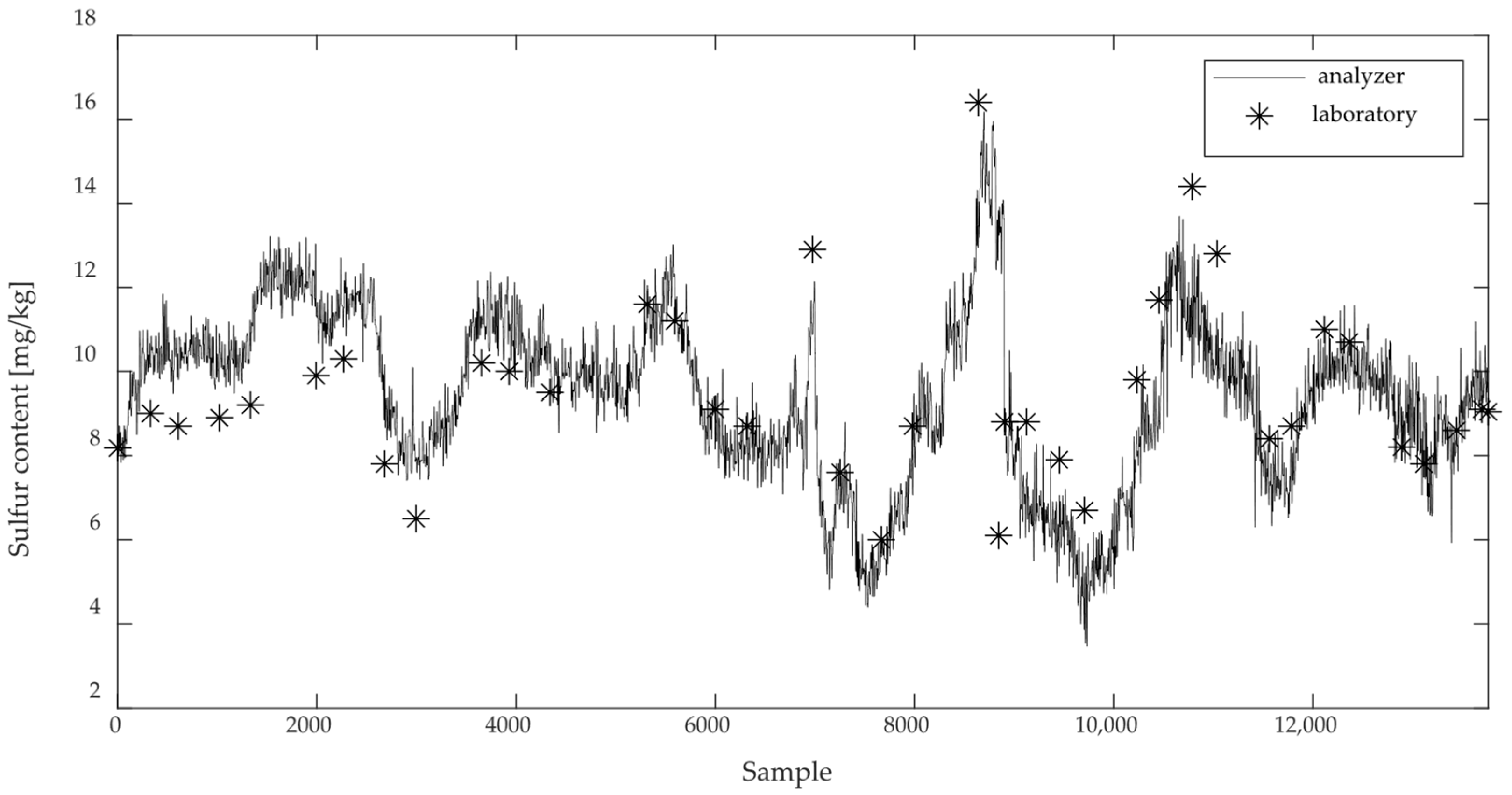
It is recommended to compare the values of the output variable (sulfur content in the product) measured by the online process analyzer with the corresponding values of the laboratory analysis. This comparison serves as the check for the correct operation of the analyzer, i.e., for the relevance of the selected data set for model development. Figure 7 shows a comparison of laboratory analysis data and online analysis data.

It can be noted that the values of the online analyzer agree quite well with the laboratory analysis, which was performed four times a day, for the entire data set with a sampling time of 1 min. However, it is evident that the analyzer deviates strongly from the laboratory values in some areas (especially for the first 3000 data samples) and that the values sometimes exceed the standard limit for the permissible sulfur content in diesel fuel of 10 mg/kg. These findings also point to a significant challenge in choosing the relevant data period for modeling under real industrial operating conditions.

The time delays for the input variables were initially approximated according to the process knowledge and experience of the plant operators. Although precise delay determination typically requires dedicated testing, such procedures are rarely feasible in full-scale industrial plants without affecting product quality. Therefore, the actual delay values used in the dynamic polynomial models, represented as nk parameters in the model structure equations [1,2,3,4], were identified and fine-tuned through a systematic trial-and-error approach using validation-based performance metrics. The final delay values (in minutes and sample steps) are summarized in

Table 6. Time delays.

№	Tag	Delay [min]	nk
1	TC-0443	3	1
2	TC-0701	15	5
3	FC-0401	12	4
4	TC-0446	12	4
5	TC-0493	12	4
6	TI-0495	9	3

, assuming a sampling period of three minutes.

The development of the model is intended for real-time estimation of the current sulfur content in the product based on delayed input variables rather than for predicting future values. The model development would require a completely new optimization of the model structure parameters for a possible prediction performance.

2.3.1. Dynamic Polynomial Models

The models were developed using the MathWorks MATLAB^® System Identification Toolbox^TM, ver. 2015a. The values of the model structure parameters na, nb, and nf were evaluated over the range of 0 to 12. This range was selected based on previous research and is empirically consistent with the dynamics of the process, the reasonable time required to compute the model, and the model complexity. The parameter nk is fixed to certain values of time delays for the selected influencing variables, as shown in Table 6. In the case of nonlinear models, parameter n, which represents the number of nonlinear units, was also examined in the range of 0 to 12. Taking these ranges into account, the model structure parameters, including na, nb, nf and the parameter n, were selected by a systematic trial-and-error procedure. Different combinations of these parameters, including fixed nk for all models, were iteratively tested and the final values were selected based on model performance indicators such as the correlation coefficient (“FIT”) between the model predictions and the measured data, and residual analysis using validation data set. The finally selected model structure parameters are listed in

Table 7. Dynamic polynomial model structure parameters.

Parameter *	FIR	ARX	OE	NARX	HW
na	–	11	–	12	–
nb	[0 3 3 12 3 3]	[10 10 10 10 10 10]	[11 11 11 11 11 11]	[12 12 12 12 12 12]	[5 5 5 5 5 5]
nf	–	–	[10 10 10 10 10 10]	–	–
n	–	–	–	10 (sigmoidnet)	[2 2 2 2 2 2] 2 (s.net)

* The parameter nk is set to [1 5 4 4 4 3] for each model and is listed separately in Table 6.

.

When developing linear parametric polynomial models, it is recommended to remove the linear trends of the measured input and output data. The linear trends were removed using the least squares method.

The continuous 4585 data samples were divided into two groups. The first 2967 data samples were used for model development and the rest for validation.

After determining the optimal order of the model by choosing the optimal parameters, the final model is obtained by calculating the optimal coefficients of the polynomial matrices of the model. The coefficients were calculated using optimization algorithms integrated into the MATLAB^® software package, ver. 2015a, based on the least squares method (for FIR and ARX), numerical search algorithms (for OE) and combinations of Gauss–Newton, Levenberg–Marquardt and trust-region optimization methods (for NARX and HW) [35].

2.3.2. ANN Models

The neural network consisted of an input layer, followed by one or more hidden layers with nonlinear activation functions (rectified linear unit—ReLU or hyperbolic tangent–tanh) and a single output layer that continuously generates an output value. The final number of hidden layers and the number of neurons per layer were selected using hyperparameter optimization. The model was trained using the ADAM (adaptive moment estimation) optimization algorithm, which uses adaptive learning rates and gradient-based updates. The loss function used in training was the mean squared error (MSE), and the model learned the layer weights by forward propagation and backpropagation of the error.

Prior to training, the input features were standardized using z-score normalization. The data samples were randomized and split into a training and test set in proportion as in dynamic polynomial models, while the predictions were later reconstructed and evaluated in chronological order. The model was developed using Python 3.9.6 programming language paired with Keras Tuner library 2.13.1. To optimize the model architecture—e.g., the number of hidden layers, the number of neurons per layer, the activation functions and the learning rate, a random search strategy within K. Tuner was used, as the problem complexity did not require a more robust hyperparameter optimization method such as the Hyperband optimization algorithm.

2.3.3. LSTM and GRU Networks

Although the static ANNs in this case study can provide satisfactory results, the application of LSTM is usually used to improve the potential for capturing temporal dependencies, as the process data from the plant environment is dynamic.

Modeling the dynamic behavior in the HDS process plant, an LSTM neural network was implemented in Python 3.9.6 programming language with TensorFlow and Keras libraries. The input process variables were standardized (z-score) and transformed into supervised learning sequences with a sliding time window of 100 samples due to the slow dynamics of the process. The data set was split into a training and test data set in proportion as in dynamic polynomial models, keeping the chronological order to reflect realistic plant conditions.

The LSTM hyperparameters were initially optimized using random search and then using the Keras Tuner library with the Hyperband search strategy. The hyperparameter space included the number of LSTM layers (2–3), the number of units per layer (128–256), the dropout rates (0.1–0.3), the L2 regularization coefficients (0.00001–0.001), the activation functions in the output layer (tanh or sigmoid), and the learning rates (0.0001–0.01). Batch normalization was applied after each LSTM layer to stabilize the training.

In the output layer, nonlinear activation functions were tested instead of the default linear setting to improve the representation of bounded target values. The model was trained with the ADAM optimizer and a batch size of 32, using early stopping to prevent overfitting.

A GRU model was also developed and tuned using both random and Hyperband optimization strategies to eventually improve the overall performance achieved by the LSTM model.

2.3.4. Model Validation

The performance of the models developed was evaluated using four statistical indicators: the Pearson correlation coefficient (R), the coefficient of determination ($R^2$), the root mean square error (RMSE), and the mean absolute error (MAE) (Equations (10)–(13)):

$$R={\displaystyle \frac{{\displaystyle \sum (x_i–\overline{x})}(y_i–\overline{y})}{\sqrt{{\displaystyle \sum {(x_i–\overline{x})}^2{\displaystyle \sum {(y_i–\overline{y})}^2}}}}};$$

(10)

$$R^2=1–{\displaystyle \frac{{\displaystyle \sum {(y_i–{\widehat{y}}_i)}^2}}{{\displaystyle \sum {(y_i–\overline{y})}^2}}};$$

(11)

$$RMSE=\sqrt{{\displaystyle \sum _{i=1}^n{({\widehat{y}}_i–y_i)}^2/n}};$$

(12)

$$MAE={\displaystyle \frac{1}{n}}{\displaystyle \sum _{i=1}^n\left|{\widehat{y}}_i–y_i\right|},$$

(13)

where $x_i$ is the measured input, $y_i$ is the measured output, ${\widehat{y}}_i$ is the model output, $\overline{x}$ is the mean of all measured inputs, $\overline{y}$ is the mean of all measured outputs, and n is the number of values in the observed data set.

All the developed models were evaluated using the same evaluation criteria (R, $R^2$, RMSE, MAE) based on the entire data set and the test set so that the developed models can be compared and interpreted. The models were also evaluated and interpreted in the form of graphical representations showing the comparison between the measured data and the model estimate of the sulfur content. The models were additionally evaluated using the histograms of the model residuals. It should be noted that all models were developed with the same number of training and test samples (2967 for training and 1618 for testing), which ensures a consistent evaluation.

3. Results

Table 8. Comparison between different types of model evaluation results for the estimation of sulfur content based on the entire data set.

Model	R (Entire)	${\mathit{R}}^2$ (Entire)	RMSE (Entire) [mg/kg]	MAE (Entire) [mg/kg]
FIR	0.730	0.531	1.330	1.083
ARX	0.811	0.655	1.141	0.924
OE	0.829	0.541	1.316	0.984
NARX	0.795	0.582	1.255	1.068
HW	0.740	0.471	1.413	1.059
ANN	0.973	0.945	0.456	0.326
LSTM	0.686	0.378	1.532	1.224
GRU	0.706	0.452	1.450	1.072

and

Table 9. Comparison between different types of model evaluation results for the estimation of sulfur content based on the test data set.

Model	R (Test)	${\mathit{R}}^2$ (Test)	RMSE (Test) [mg/kg]	MAE (Test) [mg/kg]
FIR	0.556	−0.341	2.079	1.657
ARX	0.797	0.325	1.476	1.245
OE	0.878	0.313	1.488	1.323
NARX	0.817	0.621	1.105	0.951
HW	0.884	0.739	0.917	0.705
ANN	0.969	0.939	0.472	0.323
LSTM	0.785	−0.041	1.832	1.573
GRU	0.765	0.068	1.733	1.452

show the results of all the models developed, based on evaluation criteria, while Figure 8 shows a graphical comparison between the measured data and the data obtained from the models for an estimation of the sulfur content.

In the following subsections, the model results are interpreted in relation to Table 8 and Table 9, and Figure 8.

3.1. Dynamic Polynomial Models

The FIR model is the simplest dynamic polynomial linear model. Due to its inherently simple structure, the results obtained with this model are generally unsatisfactory. When evaluating the model using the graphical representation of the entire data set (Figure 8a), it can be seen that the model follows the trend of the measured values, although local extreme values are present. The associated error values (RMSE and MAE) are relatively large, even if the model is evaluated on the entire and test data set separately.

Compared to the FIR model, the ARX model has a more complex structure, as it incorporates previous values of the measured output as input for the model, so it delivers significantly better results with smaller prediction errors. The graphical representation (Figure 8b) shows that the model follows the trend of the measured values, without a pronounced systematic error and without local extremes.

The OE model also takes into account the past values of the estimated output variable, resulting in a structure that is more complex than that of all linear polynomial models. Its results are similar to those of the ARX model, however its advantage is that it does not use the measured values of past outputs for evaluation, so its applicability is much more widely acceptable. Comparison between measured data and the sulfur content OE model result is presented in Figure 8c.

As for the NARX model, the error values when the model was evaluated on the entire data set are slightly higher compared to the ARX model. However, when it was evaluated on the test set, the NARX results are slightly better. One of the possible reasons why the much more complex NARX model generally does not perform much better could be the possibility of a pronounced linearity of the process, so that the use of nonlinear models does not have much effect. Comparison between measured data and sulfur content OE model result is presented in Figure 8d.

HW, as the most complex nonlinear dynamic model, proved to be very good in estimation, especially when considering the evaluation results on the test set. Its results in regard to this set are significantly better compared to its linear equivalent, the OE model. Compared to the OE model, it proved to be slightly worse in the evaluation for the entire set. This is also visible in the graphical representation. One of the reasons for this could be, as with the NARX model, that the use of nonlinear models does not have a large effect. Comparison between measured data and sulfur content OE model result is presented in Figure 8e.

3.2. ANN Models

Based on statistical criteria and graphical comparisons (Figure 8f), it is shown that the MLP ANNs model follows the target output variable more accurately compared to dynamic polynomial models. This improvement in performance can be attributed to the randomized training data for ANNs development, which allows it to generalize better and capture more complex patterns in the data. From the plant operator’s and application perspective, the modeling methodology is ultimately secondary as long as the model serves its purpose, i.e., has a high prediction accuracy. In this case, the static ANNs model structure has a clear advantage. Its ability to capture nonlinearities, although it lacks explicit temporal dynamics, underlines its structural complexity and flexibility compared to simpler dynamic polynomial models.

The final architecture of the neural network was selected by tuning the hyperparameters using the random search method, without the need for a more robust optimization algorithm. The optimal configuration included three hidden layers with the following number of neurons: 140, 40, and 50, respectively. The activation function tanh was chosen for all hidden layers, and the model was trained using the ADAM optimizer with a learning rate of 0.01. With this combination of hyperparameters, the best prediction performances based on validation criteria, both on the entire and test data sets, were achieved.

Table 10. The best hyperparameters determined for the ANN model developed.

Hyperparameter	Feature
Number of hidden layers	3
Number of neurons in the 1st hidden layer	140
Number of neurons in the 2nd hidden layer	40
Number of neurons in the 3rd hidden layer	50
Activation function	tanh
Optimization algorithm	ADAM
Learning rate	0.01

shows the best hyperparameters determined for the ANN model developed.

3.3. LSTM and GRU Networks

An important consideration is that data randomization was avoided during training of the LSTM, GRU, and dynamic polynomial models, as their architectures rely on preserving the temporal sequence of input data. The LSTM model showed some generalization capabilities by accurately predicting the values of sulfur content for unseen data.

Although the model was able to follow the general dynamics of the process, its performance (both in terms of the entire and test data set) did not exceed that of the static ANNs or dynamic polynomial models (excluding FIR).

This can be attributed to the relatively low complexity of the process, which does not exhibit strong nonlinearity or long-term dependencies. Therefore, simpler models such as OE, which rely on inputs and their own past predictions, were sufficient to describe the system behavior.

Table 11. The best hyperparameters determined for the LSTM model developed.

Hyperparameter	Feature
Number of LSTM layers	2
Number of units in the 1st layer	48
Number of units in the 2nd layer	48
Return sequences in the 1st layer	true
Return sequences in the 2st layer	false
Dropout rate in the 1st layer	0.5
Dropout rate in the 2st layer	0.3
Number of units in output layer	1
Activation function	linear
Optimization algorithm	ADAM
Learning rate	0.01

shows the best hyperparameters determined for the LSTM model developed.

The GRU architecture achieved comparable results, suggesting that the temporal complexity of the process does not require the longer memory capacity of LSTM cells. In contrast to LSTM, GRU models have fewer parameters and are less computationally intensive, but still effectively model short- and medium-term temporal patterns.

A visual comparison of the predicted and measured values of the sulfur content in Figure 8g,h shows a strong alignment for both LSTM and GRU models for the most important signal trends, but also a clear smoothing of the predicted results, especially in the transition areas.

Table 12. The best hyperparameters determined for the GRU model developed.

Hyperparameter	Feature
Number of GRU layers	3
Number of units in the 1st layer	32
Number of units in the 2nd layer	32
Number of units in the 3rd layer	32
Return sequences in the 1st layer	true
Return sequences in the 2st layer	true
Return sequences in the 3rd layer	false
Activation function	tanh
Recurrent activation function	sigmoid
Number of units in 3 output layers	64/64/1
Activation function in output layers	ReLu/ReLu/linear
Optimization algorithm	ADAM
Learning rate	0.01

shows the best hyperparameters determined for the GRU model developed.

3.4. Histograms of the Model Residuals

The models were additionally evaluated using the histograms of the model residuals. Residual analysis provides a meaningful way to assess the prediction quality and generalization capability of different models. Residual histograms are used to evaluate the accuracy, spread, and bias of each developed model. They represent the frequency distribution of the prediction errors (measured vs. predicted) on the test data set. Figure 9 represents comparative analysis of residual distributions across predictive models.

The ANN model has the most compact and symmetrical residual distribution, which is closely grouped around the zero point. Since almost all residuals are within ±1 mg/kg, it has excellent predictive accuracy and minimal systematic error. Similarly, LSTM and GRU also perform well, although both have a slight right skew and positive bias, indicating a slight tendency to underpredict.

The residuals of NARX are narrowly distributed but slightly positively skewed, with most errors within ±1.5 mg/kg. ARX and FIR show a broader but balanced distribution. Their scatter is wider than that of the ANNs-based models, but the symmetry and concentration suggest reliable, albeit less precise, performance.

The HW model provides residuals with significantly larger scatter, indicating occasional large deviations in prediction. OE performs worst with a flat, broad residual distribution of about −6 to +6 mg/kg, indicating high variance and instability.

Overall, the residual histograms provide additional insights into model performance beyond the scalar error metrics. The ANNs model clearly stands out for its accuracy and stability, while models such as OE and HW may need to be further optimized or reconsidered for use.

4. Discussion

The aim of this work was to compare different data-driven models based on previously explored structures, such as polynomial dynamic models, through static ANN models, to recently widely used dynamic neural networks such as LSTM and its GRU version networks, for the estimation of sulfur content in the industrial process of hydrodesulfurization.

There is no doubt that static ANNs have proven to be the most successful according to all the criteria presented.

Although the investigated process exhibits some transient behavior, the application of randomized feedforward ANNs (via data shuffle) is justified. In this approach, the model when trained is exposed to a wide range of process dynamics during training so that it can effectively learn an average behavior across different operating states. Such static models are particularly efficient when short-term memory effects are negligible or when the current process inputs contain sufficient information to predict the results. Furthermore, compared to recurrent models, they are computationally simpler and more robust against overfitting, especially when the amount of data is limited.

The relatively modest performance gain of advanced recurrent models (LSTM, GRU) over simpler models such as OE or ARX suggests that the underlying process does not exhibit pronounced nonlinear dynamics or long-term memory effects. Consequently, the OE models slightly outperformed all other models in terms of accuracy and generalization while remaining simple and interpretable.

However, OE and other recursive models are sensitive to signal dropouts and missing input data, which can temporarily destabilize their predictions. In contrast, static neural networks, which rely only on the current input vector, offer a more robust solution to data loss. Although dynamic models offer certain advantages, the quality and availability of the input signals must be taken into account when using them in industrial practice.

The relatively good performance of the OE and HW models in this case study can be attributed to the relatively low complexity of the underlying process dynamics. The system does not exhibit pronounced nonlinear behavior or highly complex temporal dependencies; therefore, simpler models such as OE, which rely solely on current inputs and their own past predicted outputs, are sufficient to capture the prevailing patterns in the data. In contrast, more advanced architectures such as NARX, HW, or LSTM are specifically designed to handle processes characterized by high dynamics and long-term dependencies that do not seem to be required in the current application. As a result, these more complex models may tend to over-fit or not provide a significant performance advantage over OE-based approaches.

However, it should be noted that OE models are inherently recursive, making them susceptible to transient signal loss or missing input values. In such scenarios, their dependence on predicted outputs can lead to error accumulation and short-term instability. To address this limitation, static neural network models are a viable and robust alternative. Since they base their predictions solely on the current input vector and do not rely on recursive state feedback, they are inherently more resilient to transient data gaps and input noise or outliers.

In addition to comparing the predictive performance of individual models, the modeling approach also included a systematic feature analysis, as well as sensitivity to sampling frequency, which helped define optimal preprocessing settings. Although a detailed computational cost analysis was not the primary goal, the relative simplicity and speed of training of static ANN and ARX models make them particularly attractive for practical industrial deployment. Compared to hardware analyzers, the proposed soft sensors offer a low-cost alternative that can provide reliable sulfur content estimation during analyzer downtime or maintenance.

The superior performance of the ANNs model is attributed to its ability to capture complex nonlinear relationships with less sensitivity to sparse data, combined with a simpler structure and fewer trainable parameters compared to LSTM and GRU. This makes it particularly suitable for processes such as HDS, which are characterized by limited data availability, moderate dynamics, and stable control conditions.

Finally, it can be emphasized that it would be advisable to apply ANNs to the HDS process under study, as they have not only been shown to be the most suitable for predicting the sulfur content in this case, but also have a robust structure that is not affected by the relatively small changes in dynamics that are to be expected in a process that is not particularly dynamic. Due to its simple structure, the polynomial dynamic model can also be considered, especially when it comes to replacing the online process analyzer when it is no longer in use. Furthermore, the implementation of the soft sensor models discussed in this work can be extended to support inferential process control strategies, enabling improved process monitoring and control based on indirect measurements.

5. Conclusions

This study presents the development and evaluation of intelligent soft sensor models for inferential monitoring of sulfur content in the hydrodesulfurization (HDS) process. Linear (FIR, ARX, OE) and nonlinear (NARX, Hammerstein–Wiener) system identification models were developed alongside machine learning approaches, including static artificial neural networks (ANNs), long short-term memory (LSTM), and gated recurrent unit (GRU) networks. Among the models tested, static ANNs demonstrated the highest prediction accuracy, while OE and HW models offered robust performance with interpretable structures. Although LSTM and GRU networks captured temporal dependencies, their added complexity yielded only marginal improvements due to the relatively low dynamic complexity of the process. The proposed soft sensor models can serve as backups during analyzer downtime and offer potential for integration into inferential process control systems.

Future research could include developing models for the HDS process by exploring other machine learning methods, such as convolutional neural networks, support vector machines, particle swarm optimization, etc., to choose the optimal model structure with respect to the application. In addition, the predictive capabilities of the developed models could be investigated.

References

1. Directive (EU) 2016/802 of the European Parliament and of the Council of 11 May 2016 Relating to a Reduction in the Sulphur Content of Certain Liquid Fuels (Codification). Available online: https://eur-lex.europa.eu/eli/dir/2016/802/oj (accessed on 15 June 2025).
2. Kadlec, P.; Gabrys, B.; Strandt, S. Data-driven soft sensors in the process industry. Comput. Chem. Eng. 2009, 33, 795–814. [Google Scholar] [CrossRef]
3. Fortuna, L.; Graziani, S.; Rizzo, A.; Xibilia, M.G. Soft Sensors for Monitoring and Control of Industrial Processes (Advances in Industrial Control); Springer: London, UK, 2007. [Google Scholar] [CrossRef]
4. Seborg, D.E.; Edgar, T.F.; Mellichamp, D.A.; Doyle, F.J., III. Process Dynamics and Control, 4th ed.; Wiley: Hoboken, NJ, USA, 2016. [Google Scholar]
5. Ljung, L. System Identification: Theory for the User, 2nd ed.; Prentice Hall: Hoboken, NJ, USA, 1999. [Google Scholar]
6. Graves, A. Supervised Sequence Labelling with Reccurent Neural Networks; Springer: Berlin/Heidelberg, Germany, 2012. [Google Scholar] [CrossRef]
7. Hochreiter, S.; Schmidhuber, J. Long Short-Term Memory. Neural Comput. 1997, 9, 1735–1780. [Google Scholar] [CrossRef]
8. Oğuz, A.; Ertuğrul, Ö.F. Introduction to deep learning and diagnosis in medicine. In Diagnostic Biomedical Signal and Image Processing Applications with Deep Learning Methods; Polat, K., Öztürk, S., Eds.; Elsevier: Amsterdam, The Netherlands, 2023; pp. 1–40. [Google Scholar] [CrossRef]
9. Li, R.; Zeng, D.; Li, T.; Xie, Y.; Hu, Y.; Zhang, G. Dynamic prediction of sulfur dioxide concentration in a single-tower double-circulation desulfurization system based on chemical mechanism and deep learning. Eng. Appl. Artif. Intell. 2025, 148, 110294. [Google Scholar] [CrossRef]
10. Zhang, H.; Wu, Z.; Yuan, Q.; Guo, L.; Li, X.; Hua, C.; Lu, P. Control of extractive dividing wall column using model predictive control based on long short-term memory networks. Sep. Purif. Technol. 2025, 361, 131351. [Google Scholar] [CrossRef]
11. Xu, Y.; Yang, G.; Li, B.; Wu, Z.; Zhao, Z.; Wang, Z. Flow inferential measurement for proportional control valves by combining wavelet denoising and a dual-attention-based LSTM network. Flow Meas. Instrum. 2024, 100, 102713. [Google Scholar] [CrossRef]
12. Prince; Yoon, B.; Kumar, P. Fault Detection and Diagnosis in Air-Handling Unit (AHU) Using Improved Hybrid 1D Convolutional Neural Network. Systems 2025, 13, 330. [Google Scholar] [CrossRef]
13. Cheng, S.; Che, Z.; Tong, Y.; Li, G.; Yue, T. Design and application of a hybrid predictive control framework for carbon capture in pressurized circulating fluidized bed coal-fired processes. Energy 2025, 322, 135701. [Google Scholar] [CrossRef]
14. Morales Matamoros, O.; Takeo Nava, J.G.; Moreno Escobar, J.J.; Ceballos Chávez, B.A. Artificial Intelligence for Quality Defects in the Automotive Industry: A Systemic Review. Sensors 2025, 25, 1288. [Google Scholar] [CrossRef]
15. Mukherjee, A.; Adeyemo, S.; Bhattacharyya, D. All-nonlinear static-dynamic neural networks versus Bayesian machine learning for data-driven modelling of chemical processes. Can. J. Chem. Eng. 2025, 103, 1139–1154. [Google Scholar] [CrossRef]
16. Pullanikkattil, S.; Yerolla, R.; Besta, C. Enhanced cryogenic distillation column identification for methane separation: A hybrid artificial neural network approach. Chem. Prod. Process Model. 2025, 20, 111–128. [Google Scholar] [CrossRef]
17. Goiburú, J.; Vera, J.; Mareco, E.F.; Pinto-Roa, D.P. Identification of Liquid-Level Systems in Industrial Processes Through Artificial Neural Networks. In Proceedings of the International Conference on Communication and Computational Technologies, Jaipur, India, 8–9 January 2024. [Google Scholar] [CrossRef]
18. Bahrun, M.H.V.; Bono, A.; Othman, N.; Zaini, M.A.A. Neural network-assisted multi-objective optimization of dual-reflux pressure swing adsorption in biogas upgrading. J. Chem. Technol. Biotechnol. 2025. [Google Scholar] [CrossRef]
19. Antosz, K.; Knapčíková, L.; Husár, J. Evaluation and Application of Machine Learning Techniques for Quality Improvement in Metal Product Manufacturing. Appl. Sci. 2024, 14, 10450. [Google Scholar] [CrossRef]
20. Laadissi, E.M. Enhancing battery system identification: Nonlinear autoregressive modeling for Li-ion batteries. Int. J. Electr. Comput. Eng. 2024, 14, 2449–2456. [Google Scholar] [CrossRef]
21. Alhanouti, M.; Gauterin, F. Predicting the Torque Demand of a Battery Electric Vehicle for Real-World Driving Maneuvers Using the NARX Technique. World Electr. Veh. J. 2024, 15, 103. [Google Scholar] [CrossRef]
22. Jiménez, J.N.; Hernández, M.M.; Alabazares, D.L.; Rabhi, A.; Pegard, C.; García, E.T. Identification Based Hammerstein-Wiener Neural Network for Propeller Pendulum PID control. In Proceedings of the 2024 IEEE International Conference on Engineering Veracruz (ICEV), Boca del Río, Mexico, 21–24 October 2024. [Google Scholar] [CrossRef]
23. Kaya, O.; Abedinifar, M.; Feldhaus, D.; Diaz, F.; Ertuğrul, S.; Friedrich, B. System identification and artificial intelligent (AI) modelling of the molten salt electrolysis process for prediction of the anode effect. Comput. Mater. Sci. 2023, 230, 112527. [Google Scholar] [CrossRef]
24. Dias, T.; Oliveira, R.; Saraiva, P.M.; Reis, M.S. Linear and Non-Linear Soft Sensors for Predicting the Research Octane Number (RON) through Integrated Synchronization, Resolution Selection and Modelling. Sensors 2022, 22, 3734. [Google Scholar] [CrossRef]
25. Mendia, I.; Gil-López, S.; Landa-Torres, I.; Orbe, L.; Maqueda, E. Machine learning based adaptive soft sensor for flash point inference in a refinery realtime process. Results Eng. 2022, 13, 100362. [Google Scholar] [CrossRef]
26. Wang, F.; Ma, S.; Niu, Y.; Liu, Z. A NOx emission concentration prediction method for CFB unit based on one-dimensional semi-empirical model corrected by GRU network. Energy 2025, 330, 136961. [Google Scholar] [CrossRef]
27. Shokri, S.; Marvast, M.A.; Sadeghi, M.T.; Narasimhan, S. Combination of data rectification techniques and soft sensor model for robust prediction of sulfur content in HDS process. J. Taiwan Inst. Chem. Eng. 2016, 58, 117–126. [Google Scholar] [CrossRef]
28. Shokri, S.; Sadeghi, M.T.; Marvast, M.A. High reliability estimation of product quality using support vector regression and hybrid meta-heuristic algorithms. J. Taiwan Inst. Chem. Eng. 2014, 45, 2225–2232. [Google Scholar] [CrossRef]
29. Lukec, I.; Sertić-Bionda, K.; Lukec, D. Prediction of sulphur content in the industrial hydrotreatment process. Fuel Process. Technol. 2008, 89, 292–300. [Google Scholar] [CrossRef]
30. Salvatore, L.; De Souza, J.; Campos, M. Design and Implementation of a Neural Network Based Soft Sensor to Infer Sulfur Content in a Brazilian Diesel Hydrotreating Unit. Chem. Eng. Trans. 2009, 17, 1389–1394. [Google Scholar] [CrossRef]
31. Cerić, E. Nafta, Procesi i Proizvodi; IBC, d.o.o.: Sarajevo, Bosnia and Herzegovina, 2012. [Google Scholar]
32. An Overview of Hydrotreating. Available online: https://www.aiche.org/resources/publications/cep/2021/october/overview-hydrotreating (accessed on 22 June 2025).
33. Beale, M.H.; Hagan, M.T.; Demuth, H.B. Deep Learning ToolboxTM User’s Guide; The MathWorks: Natick, MA, USA, 2020; pp. 53–64. [Google Scholar]
34. Zarzycki, K.; Ławryńczuk, M. LSTM and GRU Neural Networks as Models of Dynamical Processes Used in Predictive Control: A Comparison of Models Developed for Two Chemical Reactors. Sensors 2021, 21, 5625. [Google Scholar] [CrossRef] [PubMed]
35. Ljung, L. System Identification ToolboxTM User’s Guide 2014a; The MathWorks: Natick, MA, USA, 2014. [Google Scholar]
Figure 1. General process diagram of the HDS process [32].
Actuators 14 00410 g001
Figure 2. A multilayer perceptron artificial neural network structure [6].
Actuators 14 00410 g002
Figure 3. A standard LSTM unit structure [7,33].
Actuators 14 00410 g003
Figure 4. A standard GRU structure [34].
Actuators 14 00410 g004
Figure 5. Pearson correlation matrix between all potentially input variables.
Actuators 14 00410 g005
Figure 6. Process flow diagram of the reactor and stripper sections.
Actuators 14 00410 g006
Figure 7. Comparison of laboratory analysis data and online analysis.
Actuators 14 00410 g007
Figure 8. Comparison between measured data and sulfur content model results: (a) FIR; (b) ARX; (c) OE; (d) NARX; (e) HW; (f) ANN; (g) LSTM; (h) GRU.
Actuators 14 00410 g008
Figure 9. Histograms of the model residuals: (a) FIR; (b) ARX; (c) OE; (d) NARX; (e) HW; (f) ANN; (g) LSTM; (h) GRU.
Actuators 14 00410 g009aActuators 14 00410 g009b