Abstract
To further improve machining accuracy under the constrained conditions of multi-axis dynamic response, current research is focusing on the control of CNC machine toolpaths, with contour error as the target. While extant approaches analyze positions solely at PLC sampling nodes, they neglect inter-sample toolpath fluctuations induced by velocity deviations. This paper proposes a servo state-based polynomial interpolation model predictive control that predicts real-time toolpath behavior by utilizing servo axis states. The polynomial interpolation of servo states (e.g., position/velocity feedback) enables high-fidelity toolpath prediction between PLC nodes, overcoming the limitation imposed by the sampling gap. Experimental validation on a five-axis motion platform with S-shaped trajectories demonstrates that, without extending the prediction horizon of the model predictive control method, the proposed method reduces contour error by approximately 20% at the tool tip and 40% in tool orientation, while decreasing contour error fluctuations by around 60% compared to conventional model predictive control method.
1. Introduction
High-speed and high-precision machining remains a perpetual pursuit in mechanical manufacturing. With rapid advancements in aerospace, energy, and power technologies, demand has surged for high-performance components with complex curved surfaces [1], such as turbine blades and bladed disks. Given these components’ critical roles in related fields, increasingly stringent contour accuracy requirements have been imposed to ensure their performance reliability. Early CNC systems focused on tracking-error minimization to improve motion toolpath accuracy but now fail to meet high-precision machining demands. Unlike tracking error, contour error—defined as the minimum distance from the current position to the desired toolpath—better characterizes toolpath control precision [2]. Theoretically, the contour error will be reduced to zero when thetracking error reaches zero, under ideal control conditions. However, due to the compounded effects of thermal distortion (thermal errors), structural deflection under static load (elastic errors), dynamic deformation under cutting forces (dynamic errors), and inherent motion control limitations (servo mismatch, interpolation delays, etc.), it is difficult to completely eliminate axis-wise tracking errors in multi-axis CNC systems [3]. These persistent errors inevitably lead to contour deviations, especially in high-speed or high-precision machining tasks, thereby necessitating explicit contour error modeling and compensation.
In this context, achieving high precision and smoothness in toolpath generation has become increasingly important. To this end, spline interpolation techniques, particularly B-spline and NURBS, have gained wide application in modern CNC systems owing to their superior continuity and flexible control over geometric shapes. For example, Sencer et al. [4] and Liang et al. [5,6] employed cubic B-splines to represent feedrate profiles, and determined time-optimal planning by iteratively modifying the spline control points under multi-constraint conditions. In another study, Fleisig and Spence [7] introduced a spherical B-spline interpolator for computing orientation vectors in multi-axis toolpaths, enabling near-constant feedrate motion while effectively reducing rotational acceleration.
Complementary to this, enhancing contour accuracy without further improving single-axis tracking precision has become a key research focus. Current approaches fall into two categories: contour error modeling and contour error control.
In practice, the reference interpolated toolpath provided by the CNC interpolator directly influences the magnitude and variation rate of contour error. Conventional linear and circular interpolation methods often result in interpolated toolpath discontinuities in acceleration or jerk, which may cause abrupt changes in servo command and compromise contour accuracy. To address this issue, spline interpolation techniques, such as B-spline and NURBS interpolation, have been extensively studied to generate smoother interpolated toolpaths with continuous higher-order derivatives. These methods not only improve the motion continuity and reduce the excitation of mechanical vibrations but also provide a more stable basis for contour error modeling and control, particularly in high-speed and multi-axis machining scenarios. Accordingly, incorporating spline-based interpolation into the contour control framework has become an important consideration in recent research efforts.
In contour error modeling, the acquisition of precise computational models for complex desired toolpaths in actual machining remains challenging. Consequently, approximate models are predominantly adopted for contour error control. Extensive research has focused on developing such approximation methods: Cheng et al. [8] modeled contour error as the perpendicular distance from the actual position to the tangent line at a reference point. Subsequently, Yang [9] and Chen et al. [10] enhanced this approach by utilizing the osculating circle at the reference point, establishing an explicit relationship between interpolated acceleration and contour error to facilitate contour-constrained feedrate planning. Zhu et al. [11] further advanced the field by employing second-order Taylor expansion based on differential geometry to approximate multi-axis spatial point-to-curve distances. Yang [12] introduced a generalized Jacobian matrix derived from screw theory to enable real-time contour error estimation through coordinate transformations. However, it should be noted that the validity of these approximate methods is contingent upon the tracking error being small. In order to address this shortcoming, Huo et al. [13] proposed a two-stage estimation method involving nearest reference point identification prior to local contour error computation. While Hu et al. [14] formulated an orthogonal global curvilinear coordinate system for efficient planar contour error estimation, its applicability remains constrained for free-form curves due to algebraic description requirements. In the domain of five-axis toolpath control, Pi et al. [15] estimated the multi-axis contour error by using the Ferguson curve to approximate the curve between the interpolation points. Sencer et al. [16] decoupled contour error into tool-tip and orientation components. However, this method neglected coupling effects by employing spatially non-coincident reference points. Khalick and Uchiyama [17] resolved this limitation through a synchronization strategy between tool-tip position and orientation vectors. Recent innovations include Liu et al. [18] applying Taylor series expansions within the Frenet framework with curvature and torsion considerations, and Kang et al. [19] developing a high-order estimation scheme featuring fourth-order convergence for enhanced computational robustness and efficiency.
In the field of contour error control, methodologies can typically be categorized into three distinct approaches: feedback compensation control, feedforward control, and model predictive control (MPC). The feedback compensation process is initiated with an approximate estimation of the current contour error based on the actual feedback positions of each axis and the reference toolpath. Subsequently, compensation values are applied as additional commands distributed across the axes. Koren [2] pioneered the Cross-Coupled Control (CCC) strategy, which significantly enhances contour accuracy. To further improve CCC performance, researchers have integrated advanced control techniques with traditional CCC, developing variants such as: variable-gain control [20], iterative learning control [21,22], fuzzy control [23,24], and sliding mode control [24,25,26]. While CCC offers the advantages of structural simplicity and stability, its implementation in five-axis machine tools faces challenges due to rotational axis-induced nonlinearities. These complexities complicate parameter tuning in CCC controllers, and the required parameters increase disproportionately with additional axes, substantially raising commissioning workloads. Moreover, a fundamental limitation of feedback-based compensation is its inherent time lag: error computation relies on data from the previous control cycle, causing control signals to always trail error generation. Consequently, errors must first manifest before compensation can occur, resulting in reactive rather than proactive error suppression.
Additionally, many research papers and books have shown significant improvements in system control performance after applying feedforward control. One key advantage of feedforward control is its ability to respond to predictable disturbances immediately, addressing the limitation of feedback control, which cannot eliminate a significant disturbance instantaneously due to its reactive nature. Kim et al. [27] designed a feedforward controller to compensate for contour errors by modifying the reference positions. Gao et al. [28] proposed an optimal disturbance rejection feedforward control algorithm for MIMO. However, since feedforward controllers are often designed based on the inverse dynamics of the controlled plant, they tend to be highly sensitive to model inaccuracies, and improper implementation may lead to stability concerns.
In some studies, pre-compensation has been applied to achieve a feedforward-like effect. Khoshdarregi et al. [29] developed a vibration avoidance and contour error pre-compensation algorithm for feed drives that predicts contour error from tracking error. The predicted contour error is then mapped to each axis for pre-compensation. Zhang et al. [30] proposed an offline method to predict and compensate contour error for spline toolpaths in five-axis machining, where error commands are compensated before being sent to servo drives. Separately, Zhang et al. [31] introduced an iterative pre-compensation scheme for axis tracking errors to reduce contour error in biaxial platforms. Wang et al. [32] analyzed causes of contour error through time-domain analysis on three-axis systems and implemented pre-compensatory control. However, pre-compensation control represents an open-loop approach for contour control, making its accuracy dependent on model precision while lacking robustness against disturbances outside the model scope [33].
Unlike conventional feedforward control, which applies precomputed control actions without real-time correction, MPC integrates a model-based prediction with feedback correction, thereby enhancing robustness against modeling uncertainties and external disturbances. MPC has emerged as a prominent toolpath control strategy in CNC systems in recent years. The core mechanism involves predicting the future behavior of system variables over a predefined horizon using dynamic models, optimizing control sequences by minimizing a cost function, and applying only the immediate control input to the system in a receding horizon optimization framework. Key advantages of MPC include [34]: (1) intuitive concept with straightforward implementation; (2) compatibility with multivariable and multi-objective scenarios; (3) flexible accommodation of nonlinearities in models; (4) efficient handling of system constraints; and (5) adaptability for application-specific improvements and extensions. Consequently, MPC has been actively integrated into contour error control methodologies.
El Khalick et al. [35] and Tang et al. [36] proposed an MPC-based contour control algorithm for biaxial platforms. Lam et al. [37] developed an MPC algorithm capable of automatically balancing contour error and machining time in dual-axis systems. Shi et al. [38] introduced a unified modeling-based MPC contour control strategy, incorporating contour error, tracking error, control increment, and position increment into the cost function to achieve multivariable cooperative optimization. Kang et al. [39] established a spatially discrete model-based MPC contour controller using machine tool states and applied it to three-axis machine tools. Liu et al. [18] leveraged the multi-step prediction capability of Generalized Predictive Control (GPC), combining it with feedback control to eliminate feedback latency for five-axis machine control. Yang et al. [40] implemented MPC for tool tip contour control in five-axis machines but considered only positional accuracy, without addressing tool orientation precision. Kornmaneesang et al. [41] presented an MPC-based contour control scheme for 5 DOF dual-arm robots, simultaneously controlling position and orientation contour errors while enhancing robustness via integral sliding mode control. These MPC-based contour control methods applied to CNC machine tools typically select small prediction horizons (e.g., merely three steps in [39] and two steps in [42] on three-axis platforms) to meet real-time requirements. Alternatively, MPC can only be implemented offline—Wang et al. [43] proposed a combined approach using offline MPC-based pre-compensation with real-time feedback control. However, offline MPC relies on simulation model states rather than actual servo axis states, leading to error accumulation.
In addition, the implementation of MPC places substantial computational demands on the control hardware, as a large number of matrix operations must be completed within each interpolation cycle. To address these challenges, researchers have explored advanced hardware platforms centered around field-programmable gate arrays (FPGAs), which have shown significant advantages over conventional hardware in terms of sampling frequency, communication latency, and control accuracy. These developments have laid a solid foundation for embedding MPC strategies into next-generation machine tools and robotic systems [44,45,46]. Notably, the recent work by Przybył highlights that [47] compared to traditional MCU/DSP+ASIC-based servo drives, FPGA-based architectures, with their inherent parallelism and on-chip real-time execution (RTE) modules, can deliver over ten times the computational headroom and significantly higher diagnostic data throughput, without incurring additional power consumption or cost.
However, the contour error approximation methods in the aforementioned literatures calculate contour error solely based on position information at PLC control cycle sampling nodes (hereafter referred to as sampling nodes). These models neglect the impact of velocity deviations from the desired toolpath on contour error. In practice, when the actual velocity deviates from the desired values, larger contour errors may occur within the control cycle compared to those at sampling nodes. This paper incorporates velocity deviations into the contour error calculation model using a polynomial interpolation approach, adding the contour error of motion toolpath between sampling nodes to the control objectives. A corresponding MPC controller is established to regulate contour error. Experimental validation with an S-shaped toolpath demonstrates the effectiveness of the proposed contour error control strategy.
The subsequent sections of this paper are organized as follows. The novel contour error evaluation method based on polynomial interpolation is described in Section 2. Section 3 introduces a specific method for controlling the proposed contour error index using the MPC method. Experimental verification is conducted in Section 4. Section 5 concludes this paper.
2. Contour Error Estimate Based on Polynomial Interpolation
In the context of CNC machining processes, adopting the contour error at sampling nodes relative to the desired toolpath as the sole criterion for contour accuracy assessment inadequately represents the toolpath’s overall contour accuracy. This limitation becomes particularly critical when velocity directions at sampling nodes exhibit significant deviations from the desired toolpath’s reference directions. Under such conditions, exclusive control of contour errors at sampling nodes may induce oscillatory motion of the actual toolpath (the toolpath synthesized from the servo axes’ dynamic responses, hereinafter referred to as “actual toolpath”) about the reference toolpath. Crucially, while high contour accuracy is maintained at sampling nodes, substantial contour errors may develop between adjacent sampling nodes. As shown in Figure 1, actual toolpath 1 demonstrates smaller contour errors at all sampling nodes than actual toolpath 2. Nevertheless, due to its larger velocity deviations at these nodes, actual toolpath 1 exhibits inferior overall contour accuracy compared to actual toolpath 2.
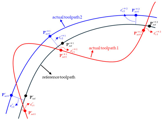
Figure 1.
Inability of contour errors at sampling nodes to represent overall toolpath contour accuracy.
Therefore, this paper proposes a contour error control strategy based on the polynomial interpolation of servo axis states. Using position and velocity data from both the desired toolpath and actual axis motion, third-order polynomial curves are interpolated to generate the toolpath profiles and , respectively. By selecting appropriate interpolation points along these contours, the controller aims to minimize the sum of squared contour errors at these points. Compared to methods regulating only contour errors at sampling nodes, this approach integrates velocity information at sampling nodes, thereby enhancing the actual contour accuracy of the motion toolpath.
Based on the motion states at two sampling nodes, the actual continuous toolpath can be approximated using a Ferguson cubic parametric equation, where the subscript r denotes the state and input parameters at time tr within the r-th PLC control cycle.
Based on position and velocity data at the r-th and (r + 1)-th sampling nodes, the actual toolpath during this control cycle () can be interpolated using a third-order polynomial expression as follows:
where the normalized parameter , defines the polynomial’s parametric domain, and the coefficient matrix is defined by:
Here, denotes the PLC control cycle of the system.
Define the interpolation operators: , and let , , where superscripts denote axis indices. Here, and represent the positions and velocities of all servo axes at the r-th sampling node.
The interpolated toolpath positions and velocities at any point can then be derived as follows:
where and denote the Kronecker products of and with the n-th order identity matrix , respectively, and n represents the number of servo axes in the system:
By comparing the desired toolpath with the actual toolpath, and employing a tangential approximation approach for the linearization of contour errors, the contour error at interpolation points can be approximated using tracking errors and unit velocity vectors:
where denotes the contour error scalar, represents the tracking error vector composed of per-axis tracking errors, and defines the velocity field vector.
Consequently, the sum of squared contour errors at multiple interpolation points between adjacent sampling nodes can be calculated as:
where
In practical applications, given that the position–velocity-based interpolation yields a third-order polynomial toolpath, selecting three interpolation points—including the endpoints—is justified as sufficient for characterizing contour accuracy. This paper specifically chooses the parameter values 1/3, 2/3, and 1.
3. State-Space Model Predictive Control Method
Section 2 introduces a contour error evaluation based on third-order polynomial interpolation. This method comprehensively integrates position and velocity tracking errors at sampling nodes to calculate the motion of the contour errors on the actual motion toolpath. Compared to conventional approaches considering only sampling-node position deviations, it achieves a more precise characterization of the overall actual toolpath contour accuracy.
State-space-based MPC enables the prediction of multi-axis states over a finite prediction horizon. When the first two state variables correspond to axis positions and velocities, respectively, they directly align with the proposed contour error calculation framework.
3.1. Servo System Dynamics Modeling
The electromechanical dynamics model for each servo axis is shown in Figure 2a. Given that the current loop bandwidth typically far exceeds those of the velocity and position loops, this study simplifies the system by approximating the current loop transfer function as unity during modeling. Consequently, the system can be reduced to the form depicted in Figure 2b. Defining the state variables as axis position, velocity, and the integral term of the velocity loop, the servo dynamics can be described by a third-order state-space equation as follows:
where
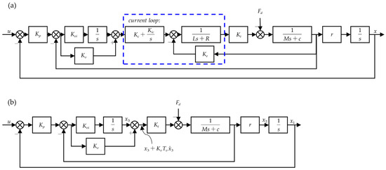
Figure 2.
Servo feed drive system control block diagram. (a) Detailed control block diagram of the servo axis. (b) Simplified control block diagram of the servo axis.
Here, and represent the proportional gain coefficient of the position loop and velocity loop, respectively. is the integral gain coefficient of the velocity loop. is the torque constant of the motor. and represent the equivalent mass and equivalent damping coefficient. Here, represents the fear ratio or reduction ratio, and is other disturbance forces besides viscous damping, including Coulomb friction, motor positioning force fluctuations, and other disturbances (such as cutting forces, etc.).
Given that the disturbance exhibits negligible variation within an interpolation period, the system described by Equation (11) can be discretized using a zero-order hold (ZOH). The resulting discrete-time system is expressed as Equation (13):
where
3.2. Contour-Error-Based Model Predictive Cost Function Construction
Assuming the discrete state-space representation of each servo axis in the system can be described in the following constant-term-included form:
where , , and denote the state vector, input, and disturbance of the system, respectively, the discrete state-space equations of individual axes can be integrated to construct a multi-axis discrete state-space representation:
where , , and . The state transition matrix, input matrix, and constant-term matrix in the equation are defined as follows:
Here, the superscripts denote the corresponding axis indices, the subscripts indicate elements at specific row/column positions in the single-axis state-space matrices, and k represents the model order of each servo axis.
Based on the discrete state-space representation, states over the next m prediction periods can be predicted through iterative computation:
where , , , , and .
When the first two states in the state-space representation correspond to axis positions and velocities, respectively, the position and velocity states at adjacent sampling nodes can be extracted to perform polynomial interpolation for the predicted actual toolpath (the predicted toolpath composed from axis responses using the state-space model):
where
Thus, the sum of squares of predicted contour errors over the prediction horizon can be calculated as follows:
where
During actual system operation, relying exclusively on contour error as the sole control objective results in the actual feedrate deviating significantly from the planned feedrate profile. This outcome clearly fails to meet practical machining requirements. Consequently, when constructing the MPC cost function for real-world implementation, tracking-error-based cost terms () must be incorporated alongside the contour error component. Furthermore, to enhance system robustness and prevent instability induced by model inaccuracies, a cost term () constraining control input adjustments should also be introduced. The corresponding cost function is structured as follows:
where
Combining Equations (21) and (23) with distinct weighting coefficients, let , , and denote the weights for the contour error, tracking error, and incremental command adjustment, respectively. This yields a quadratic cost function expressed in terms of multi-axis commands:
where
Taking the partial derivative of the control objective with respect to the optimization command vector based on Equation (25):
Setting , the optimal control command with unconstrained conditions that minimizes can be calculated as follows:
The first period’s command of this solution is extracted and transferred to the drives as the actual control command for the current control period:
4. Experimental Verification
To validate the effectiveness of the contour error modeling method proposed in Section 2 and the corresponding MPC approach in Section 3, experimental verification was conducted on a five-axis motion platform as shown in Figure 3. The X-axis is driven by dual linear motors in a synchronous bilateral configuration. A crossbeam mounted on the X-axis forms the Y-axis, which is also driven by a linear motor. The Z-axis employs a ball screw mechanism actuated by a rotary motor. On the Z-axis carriage, both the C-axis and A-axis are installed, utilizing rotary motors coupled with gear reducers for actuation. The precision and performance specifications of the experimental platform are detailed in the table provided in Appendix B.
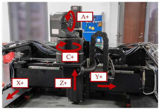
Figure 3.
Five-axis motion platform.
The motion control system operates within the Beckhoff TwinCAT 3 (v3.1.4024.56) (The Windows Control and Automation Technology 3) real-time environment, implemented using PLC Structured Text compliant with the IEC 61131-3 standard [48]. The control system runs on a Beckhoff industrial PC (Model: C6640-0040), communicating with servo drives via the EtherCAT fieldbus protocol, with a deterministic PLC control cycle of 2 ms. The servo drives are synchronized with the 2 ms PLC control cycle for command reception and execution coordination, while internally operating at higher-frequency control loops. In particular, the position control loop of each drive runs at a cycle time of 125 μs, ensuring fast and accurate actuator response.
The interpolator proposed in Reference [49] is adopted to improve interpolation efficiency. This method employs an implicit feedrate planning strategy, which directly constructs a mapping between the toolpath parameter u and the machining time t. By bypassing the nonlinear arc-length reparameterization from s to u, this approach significantly simplifies the interpolation process and reduces the computational burden during the real-time interpolation process.
4.1. Integration of the Proposed Control Method into CNC System
This section describes the integration scheme of the proposed MPC-based contour error control method into a multi-axis servo system, focusing on its real-time execution architecture. Key implementation steps—including state acquisition, interpolation, error estimation, optimization solving, and control command issuance—are coordinated within each PLC control cycle. The complete workflow of the PLC-based control system is illustrated in Figure 4.
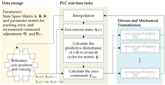
Figure 4.
The complete workflow of the proposed MPC method for PLC control system.
(1) Initialization
Before the control system starts operation, the following initialization steps are required: calculate and import the state-space matrices , , and as Equation (18), and calculate the parameter matrix for tracking error and incremental command adjustment: , .
(2) Execution Procedure in Each PLC Control Cycle
1) Toolpath Interpolation:
The fast interpolator proposed in [49] is utilized to update the interpolated positions and velocities of each axis from cycle k to k + m.
2) State Acquisition and Estimation:
Real-time feedback data including axis positions and velocities are collected to construct the system state vector for the current cycle. As the control model adopts a third-order state-space structure (as illustrated in Figure 2b), the third-order state—representing the integral component of the velocity loop—is not directly observable from the servo drives. This component is estimated based on current loop data.
As discussed in Section 3.1, the bandwidth of the current loop is typically much higher than that of the velocity and position loops, allowing the current loop dynamics to be approximated as a unity gain system. Under this simplification, the input and output of the current loop are equivalent, giving the following relationship:
At steady state, the derivative term can be neglected, leading to the initial value:
In subsequent PLC cycles, the integral state is updated using the backward Euler method:
This procedure enables the real-time estimation of the complete state vector x(k) for each axis.
3) Based on the dynamic models of each axis, the disturbance force matrix over the preview horizon is predicted and computed. The disturbances include friction forces of the servo axes, motor cogging forces, components of cutting forces along each axis, and other relevant effects.
4) The optimized commands to be sent to each axis drive are calculated based on Equations (28) and (29) and then sent to the drives.
4.2. Experimental Verification with “S”-Shaped Toolpath
The “S”-shaped piece is currently a widely adopted standard for validating five-axis machining centers, as it features complex freeform surfaces that effectively test the machine’s multi-axis coordination and contouring capabilities. Moreover, it is recommended by both ISO 10791-7:2020 [50] and GB/T 39967-2021 [51] standards for evaluating five-axis machine tool performance, allowing for the assessment of not only geometric errors but also the performance of NC and servo controllers. Therefore, the S-shaped test piece provides a general, repeatable, and standardized benchmark for the comparative evaluation of control strategies.
This paper selects a scaled toolpath derived from the surface on one side of the “S”-shaped piece (illustrated in Figure 5) as the target toolpath. The blue curve, denoted by C(u), represents the toolpath of the tool tip point(TTP) in Cartesian space, which defines the spatial path that the tool is expected to follow. The green curve, denoted by H(u), indicates the orientation toolpath of the tool axis, characterizing the directional posture of the tool along the motion path. The red connecting lines between corresponding points on C(u) and H(u) illustrate the instantaneous tool orientation vector at selected positions, i.e., the tool axis direction, forming a complete representation of both the position and orientation required for five-axis toolpath planning and control. The dual NURBS parameters for this toolpath are provided in Table A1 of Appendix A. Both simulation and experimental models of each axis and drive parameters were either identified through parameter estimation or directly obtained from the drives, as detailed in Table A2.
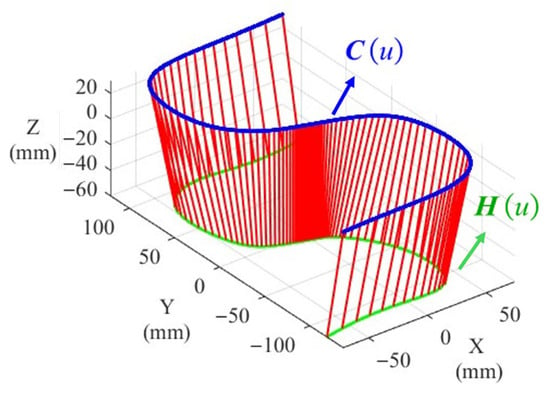
Figure 5.
The “S”-shaped piece toolpath.
Figure 6 presents the planned feedrate profiles and the corresponding axis velocity responses obtained from the experimental five-axis platform. For each axis, both the commanded (set) velocity and the actual measured (act) velocity are displayed, based on real-time data acquisition from the servo drives. The figure allows for a comparative analysis of system behavior under different control strategies. It can be observed that when using the conventional feedback control method (M3) based solely on PID, the axis velocities remain relatively smooth. In contrast, the application of the MPC-based method (M2) introduces noticeable velocity fluctuations, particularly along the X, Y and Z axes, as a result of the model-driven optimization reacting to servo mismatches. When employing the proposed method (M1), which incorporates an interpolation-based approximation of the actual toolpath and integrates axis-wise velocity deviations into the contour error model, the velocity fluctuations are significantly mitigated.
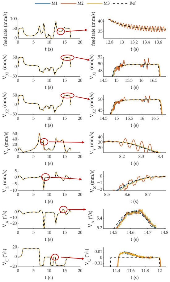
Figure 6.
Comparison between target and actual feedrate and axis velocities with local enlarged view.
Figure 7 presents a comparison between the reference and actual axis accelerations obtained using the baseline MPC approach (M2) and the proposed MPC strategy (M1). For M2, the pursuit of higher contouring accuracy inevitably induces fluctuations in both axis velocities and accelerations. In contrast, the proposed M1 formulation integrates the reference axis velocities directly into the contour error model, enabling significant suppression of unnecessary acceleration oscillations. As a result, peak loads on the drive system are effectively reduced. This additional result provides a more intuitive and quantitative validation of the proposed method’s capability to enhance motion smoothness while alleviating dynamic loading.
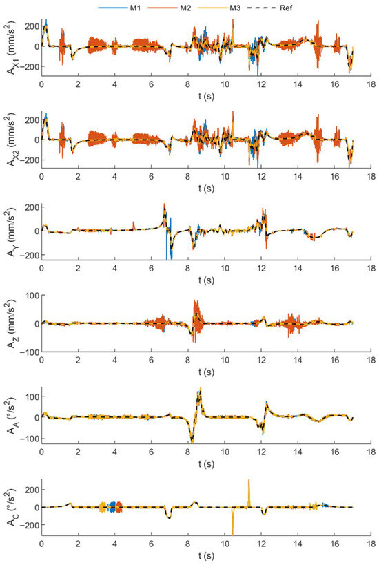
Figure 7.
Comparison between target and actual axis acceleration.
The feedrate planning for the trajectory was subject to several kinematic constraints imposed by the servo system capabilities and trajectory smoothness requirements. These include axis-specific limitations on maximum velocity, acceleration, and jerk, which are summarized in Table 1. The planning algorithm ensures that these constraints are satisfied along the entire trajectory to avoid drive saturation and maintain contouring accuracy.

Table 1.
Constraints for feedrate planning.
Based on engineering experience while balancing MPC optimization effectiveness and the real-time requirements of the NCK (Numerical Control Kernel), this paper sets the MPC prediction horizon to 4. The weights for the contour error, tracking error, and command adjustment in Equation (25) are assigned as follows: , , and , respectively. These values are determined based on engineering experience and preliminary experimental tuning to provide a balance between contour accuracy, tracking performance, and control effort. Systematic optimization of these weights is left for future work.
The proposed contour error control method based on polynomial interpolation (M1) is compared with two benchmark approaches: an MPC method that controls contour error exclusively at sampling nodes (M2), and a conventional feedback control approach (M3). Figure 8 and Figure 9 and Table 2 provide experimental validation, while the required feedrate is set to 100 mm/s. A critical analysis confirms that M1 significantly outperforms M2 in terms of contour error precision for both tool tip toolpath tracking and tool orientation control. Specifically, M1 reduces the average tool tip point contour error (TTPCE) by 23.2% and by 22.0% for average tool orientation contour error (TOCE), relative to M3. Compared with M2, M1 provides an additional improvement of around 5% in both categories. Furthermore, maximum contour error demonstrates substantial improvements: TTPCE is reduced by around 16% compared with M2 and by approximately 27% compared with M3, while TOCE decreases by around 36% and 50%, respectively.
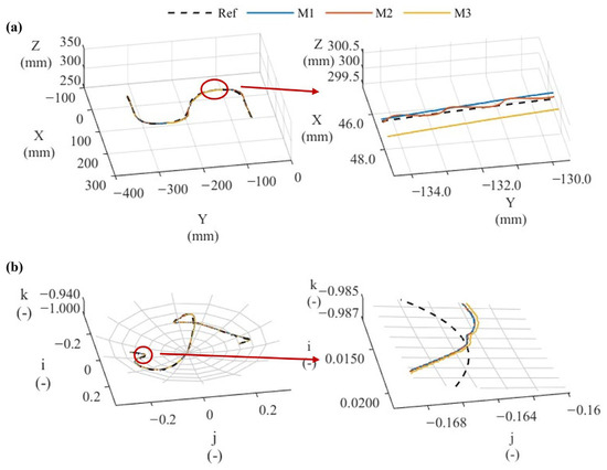
Figure 8.
Comparison of tool tip point path and tool orientation vector path results for the three methods, with separate local enlargements: (a) tool tip point path and (b) tool orientation vector path (M1: contour error control method based on polynomial interpolation; M2: MPC method that controls contour error only at sampling nodes; M3: feedback control, all actual tool tip paths and tool orientation paths shown in the figure are magnified 10 times in the direction of contour error).
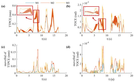
Figure 9.
Comparison of contour errors between the three methods. (a) Tool tip point contour error (TTPCE), (b) Tool orientation contour error (TOCE), (c) Moving-window standard deviation of TTPCE (moveStd of TTPCE), (d) Moving-window standard deviation of TOCE (moveStd of TOCE).

Table 2.
Comparison of results from three contour error control methods.
Furthermore, the proposed method’s incorporation of velocity errors for all axes into contour error evaluation significantly improves the fluctuation of contour error compared to position-only approaches. To quantify contour error volatility, this study uses the moving standard deviation (moveStd), which is computed within a ±100 ms window centered on each timestamp. Higheconr moveStd values indicate greater fluctuation amplitude and poorer contour precision control. As shown in Figure 9c,d and Table 1 (specifically the ‘max moveStd’ and ‘mean moveStd’ entries), the experimental results demonstrate that the proposed method substantially reduces contour error fluctuations relative to M2. The maximum and mean running standard deviations for tool tip point contour error (TTPCE) and tool orientation contour error (TOCE) are markedly lower, registering at only 36.6% and 46.6%, respectively, of M2’s values. These results confirm the effectiveness of the method in reducing actual toolpath oscillation during contour control and improving the accuracy of the final machining contour.
5. Conclusions
This paper proposes a contour error evaluation method based on polynomial interpolation that balances position control accuracy and velocity control accuracy. The contour error of the toolpath is estimated based on the position and velocity tracking errors of each motion axis. In comparison with conventional methodologies, which merely estimate tool position and orientation based on the positions of each motion axis at sampling nodes for contour control, the method proposed in this paper can evaluate the contour accuracy of the toolpath between sampling nodes. This capability aligns more closely with the actual requirements of machining processes.
Moreover, experimental verification is conducted on an actual motion control platform based on model predictive control (MPC) algorithms. In comparison with conventional contour control methodologies that are predicated on the state space of each axis, the approach delineated in this paper employs a more extensive utilization of the higher-order state variables (velocity states) of each axis, thereby ensuring enhanced stability in control performance without any augmentation in the prediction interval. This approach serves to mitigate oscillations triggered by model inaccuracies and random disturbances.
In conclusion, the ruled surface of one side of the “S”-shaped standard piece was designated as the target toolpath. Subsequently, experimental verification was conducted on a five-axis motion control platform. The results obtained are as follows:
- In comparison with feedback control or conventional contour error MPC control, the contour error control objective and corresponding MPC implementation proposed in this paper achieve improvements of approximately 20% and 40% or more in the control of the tool tip point motion path contour and tool orientation path contour, respectively.
- Compared with conventional contour error MPC methods, which typically require a limited prediction interval to satisfy the real-time demands of CNC systems, consequently resulting in stability deficiencies, the proposed method demonstrates significant advantages. The proposed methodology in this paper enhances stability by introducing contour control objectives at interpolation points without increasing the prediction interval or raising the matrix dimension of the system’s computational requirements. In experimental validation, it demonstrated significantly better stability than conventional methods. The maximum and average standard deviations of the tool tip point and tool orientation were found to be 36.6% and 46.6% and 41.7% and 65.0%, respectively, in comparison to the conventional contour error MPC method.
While reducing the control cycle time could theoretically reduce feedback delay, it often entails substantial hardware and system-level cost. In contrast, the proposed interpolation-based contour error control method improves precision without altering the servo infrastructure, thus offering a cost-effective and practical solution for existing CNC systems. Moreover, the method is fully compatible with high-end CNC platforms that already operate with shortened control cycles. In such systems, the proposed approach can serve as a complementary layer of control, offering additional precision improvement by addressing contour deviation from the interpolated toolpath planning level.
Additionally, the efficacy of the algorithm may be enhanced through the optimization of pertinent parameters. The present paper provides a set of parameters based on engineering practice to meet experimental requirements; however, it does not conduct an in-depth study on how to select the optimal parameters. This will be the focal point of future research.
Furthermore, to enhance the practical relevance and robustness of the proposed method, future research will aim to establish an experimental platform capable of conducting real machining tests. This will enable the evaluation of additional performance indicators beyond contour error, including acceleration and jerk profiles, motion smoothness, and physical part quality (e.g., surface finish and residual defects). Such validation will help quantify the impact of the control algorithm under actual machining disturbances such as cutting forces and thermal effects, thereby providing more comprehensive support for industrial applications.
Author Contributions
Conceptualization, S.L. and Q.L.; methodology, S.L. and Z.N.; software, S.L.; validation, S.L., C.Z. and L.W.; formal analysis, S.L.; investigation, S.L.; resources, Q.L. and Y.L.; data curation, S.L.; writing—original draft preparation, S.L.; writing—review and editing, Y.Y. and Y.L.; visualization, S.L.; supervision, Q.L.; funding acquisition, Y.L. All authors have read and agreed to the published version of the manuscript.
Funding
This research received no external funding.
Data Availability Statement
Data are contained within the article.
Conflicts of Interest
The authors declare no conflicts of interest.
Appendix A

Table A1.
Dual NURBS parameters of the “S”-shaped toolpath.
Table A1.
Dual NURBS parameters of the “S”-shaped toolpath.
| Parameters | Value |
|---|---|
| Order | 3 |
| C(u) control vertices (tool tip point toolpath) | (−11.625, −137, 30), (−10.75, −134, 30), (17.25, −138, 30), (65.25, −118, 30), (63, −19, 30), (43.5, −13, 30), (7.5, −11, 30), (1.5, −1, 30), (−1.5, −1, 30), (−10.5, −1, 30), (−14.5, 3, 30), (−16, 36, 30), (−13, 111, 30), (−1.75, 119, 30), (32.25, 118, 30), (74.625, 121, 30) |
| H(u) control vertices (tool axis toolpath) | (−11.625, −131, 0), (−10.75, −126, 0), (17.25, −131, 0), (58.5, −116, 0), (57.75, −11, 0), (34.5, −10, 0), (7.5, −11, 0), (1.5, −1, 0), (−1.5, −1, 0), (−10.5, −1, 0), (−14.5, 3, 0), (−10, 32, 0), (−10.75, 103, 0), (−1.75, 116, 0), (32.25, 110, 0), (74.625, 115, 0) |
| Knot vector | (0, 0, 0, 0, 0.0769, 0.1538, 0.2308, 0.3077, 0.3846, 0.4615, 0.5385, 0.6154, 0.6923, 0.7692, 0.8462, 0.9231, 1, 1, 1, 1) |
| Weight vector | (1, 1, 1, 1, 1, 1, 1, 1, 1, 1, 1, 1, 1, 1, 1, 1) |

Table A2.
Model parameters of each axis.
Table A2.
Model parameters of each axis.
| (1/s or rad/(s·m)) | 27.9926 | 28.0712 | 70.8024 | 61,718.5 | 4831.58 | 3731.66 |
| (A·s/m or A·s/rad) | 19.9087 | 19.9087 | 59.8906 | 0.536018 | 1.782 × 10⁻⁴ | 0.0329 |
| (A/m or A/rad) | 3455 | 3455 | 2506 | 1.978 | 2.227 × 10⁻³ | 0.8375 |
| (N/A or N·m/A) | 48.6 | 48.6 | 48.6 | 0.508 | 0.357 | 0.386 |
| (- or m/rad) | 1 | 1 | 1 | 0.01/(2pi) | 1/101 | 1/101 |
| (kg or kg·m2) | 25.50 | 33.80 | 22.43 | 1.246 × 10⁻⁴ | 3.143 × 10⁻⁶ | 2.253 × 10⁻⁴ |
| (N·s/m or N·m·s/rad) | 36.46 | 31.20 | 6.89 | 0.0053 | 3.07 × 10⁻⁴ | 0.2546 |
| (N or N·m) | 37.03 | 21.56 | 20.91 | 0.1845 | 1.25 × 10⁻⁴ | 0.09135 |
Appendix B

Table A3.
Precision parameters of the motion platform.
Table A3.
Precision parameters of the motion platform.
| Parameters | ||
|---|---|---|
| Axis Travel (mm or °) | X1/X2/Y/Z | 200/200/400/200 |
| A/C | ±120/±180 | |
| Positioning Accuracy (μm or ″) | X1/X2/Y/Z | 2.1/2.0/1.6/2.0 |
| A/C | 39.2/34.7 | |
| Repeatability (μm or ″) | X1/X2/Y/Z | 1.6/1.5/1.2/1.6 |
| A/C | 16.2/22.0 | |
| Max Feedrate (mm/s or °/s) | X1/X2/Y/Z | 500/500/500/200 |
| A/C | 100/150 | |
| Max Acceleration (mm/s2 or °/s2) | X1/X2/Y/Z | 8000/8000/8000/3000 |
| A/C | 1000/1500 | |

Table A4.
Motor parameters of the motion platform.
Table A4.
Motor parameters of the motion platform.
| X/Y | Z | A | C | |
|---|---|---|---|---|
| Motor Model | LMG3C-400-450 | KK86-10P-340 | SHA25P-101SG | KAH-14C |
| Encoder Type | Incremental Linear Encoder | Incremental Linear Encoder | Absolute Rotary Encoder | Absolute Rotary Encoder |
| Encoder Resolution (µm/count or counts/rev) | 0.1 | 0.1 | 220 | 217 |
| Rated Current (A) | 4.2 | 2.5 | 0.44 | 2.9 |
References
- Chen, Y.; Gao, J.; Deng, H.; Zheng, D.; Chen, X.; Kelly, R. Spatial Statistical Analysis and Compensation of Machining Errors for Complex Surfaces. Precis. Eng. 2013, 37, 203–212. [Google Scholar] [CrossRef]
- Koren, Y. Cross-Coupled Biaxial Computer Control for Manufacturing Systems. J. Dyn. Syst. Meas. Control 1980, 102, 265–272. [Google Scholar] [CrossRef]
- Gao, W.; Ibaraki, S.; Donmez, M.A.; Kono, D.; Mayer, J.R.R.; Chen, Y.-L.; Szipka, K.; Archenti, A.; Linares, J.-M.; Suzuki, N. Machine Tool Calibration: Measurement, Modeling, and Compensation of Machine Tool Errors. Int. J. Mach. Tools Manuf. 2023, 187, 104017. [Google Scholar] [CrossRef]
- Sencer, B.; Altintas, Y.; Croft, E. Feed Optimization for Five-Axis CNC Machine Tools with Drive Constraints. Int. J. Mach. Tools Manuf. 2008, 48, 733–745. [Google Scholar] [CrossRef]
- Liang, F.; Zhao, J.; Ji, S. An Iterative Feed Rate Scheduling Method with Confined High-Order Constraints in Parametric Interpolation. Int. J. Adv. Manuf. Technol. 2017, 92, 2001–2015. [Google Scholar] [CrossRef]
- Liang, F.; Yan, G.; Fang, F. Global Time-Optimal B-Spline Feedrate Scheduling for a Two-Turret Multi-Axis NC Machine Tool Based on Optimization with Genetic Algorithm. Robot. Comput.-Integr. Manuf. 2022, 75, 102308. [Google Scholar] [CrossRef]
- Fleisig, R.V.; Spence, A.D. A Constant Feed and Reduced Angular Acceleration Interpolation Algorithm for Multi-Axis Machining. Comput.-Aided Des. 2001, 33, 1–15. [Google Scholar] [CrossRef]
- Cheng, M.-Y.; Lee, C.-C. Motion Controller Design for Contour-Following Tasks Based on Real-Time Contour Error Estimation. IEEE Trans. Ind. Electron. 2007, 54, 1686–1695. [Google Scholar] [CrossRef]
- Yang, J.; Li, Z. A Novel Contour Error Estimation for Position Loop-Based Cross-Coupled Control. IEEEASME Trans. Mechatron. 2011, 16, 643–655. [Google Scholar] [CrossRef]
- Chen, M.; Xu, J.; Sun, Y. Adaptive Feedrate Planning for Continuous Parametric Tool Path with Confined Contour Error and Axis Jerks. Int. J. Adv. Manuf. Technol. 2017, 89, 1113–1125. [Google Scholar] [CrossRef]
- Zhu, L.; Zhao, H.; Ding, H. Real-Time Contouring Error Estimation for Multi-Axis Motion Systems Using the Second-Order Approximation. Int. J. Mach. Tools Manuf. 2013, 68, 75–80. [Google Scholar] [CrossRef]
- Yang, J.; Altintas, Y. A Generalized On-Line Estimation and Control of Five-Axis Contouring Errors of CNC Machine Tools. Int. J. Mach. Tools Manuf. 2015, 88, 9–23. [Google Scholar] [CrossRef]
- Huo, F.; Xi, X.-C.; Poo, A.-N. Generalized Taylor Series Expansion for Free-Form Two-Dimensional Contour Error Compensation. Int. J. Mach. Tools Manuf. 2012, 53, 91–99. [Google Scholar] [CrossRef]
- Hu, C.; Yao, B.; Wang, Q. Global Task Coordinate Frame-Based Contouring Control of Linear-Motor-Driven Biaxial Systems With Accurate Parameter Estimations. IEEE Trans. Ind. Electron. 2011, 58, 5195–5205. [Google Scholar] [CrossRef]
- Pi, S.; Liu, Q.; Liu, Q. A Novel Dynamic Contour Error Estimation and Control in High-Speed CNC. Int. J. Adv. Manuf. Technol. 2018, 96, 547–560. [Google Scholar] [CrossRef]
- Sencer, B.; Altintas, Y.; Croft, E. Modeling and Control of Contouring Errors for Five-Axis Machine Tools—Part I: Modeling. J. Manuf. Sci. Eng. 2009, 131, 031006. [Google Scholar] [CrossRef]
- El Khalick M, A.; Uchiyama, N. Estimation of Tool Orientation Contour Errors for Five-Axismachining. Robot. Comput.-Integr. Manuf. 2013, 29, 271–277. [Google Scholar] [CrossRef]
- Liu, Y.; Wan, M.; Xiao, Q.-B.; Qin, X.-B. Combined Predictive and Feedback Contour Error Control with Dynamic Contour Error Estimation for Industrial Five-Axis Machine Tools. IEEE Trans. Ind. Electron. 2021, 69, 6668–6677. [Google Scholar] [CrossRef]
- Kang, Z.; Lin, W.; Liu, Z.; Xu, R. Accurate Contour Error Estimation-Based Robust Contour Control for Dual-Linear-Motor-Driven Gantry Stages. Mechatronics 2024, 100, 103174. [Google Scholar] [CrossRef]
- Koren, Y.; Lo, C.-C. Variable-Gain Cross-Coupling Controller for Contouring. CIRP Ann. 1991, 40, 371–374. [Google Scholar] [CrossRef]
- Barton, K.L.; Alleyne, A.G. A Cross-Coupled Iterative Learning Control Design for Precision Motion Control. IEEE Trans. Control Syst. Technol. 2008, 16, 1218–1231. [Google Scholar] [CrossRef]
- Xu, W.; Hou, J.; Li, J.; Yuan, C.; Simeone, A. Multi-Axis Motion Control Based on Time-Varying Norm Optimal Cross-Coupled Iterative Learning. IEEE Access 2020, 8, 124802–124811. [Google Scholar] [CrossRef]
- Chin, J.-H.; Cheng, Y.-M.; Lin, J.-H. Improving Contour Accuracy by Fuzzy-Logic Enhanced Cross-Coupled Precompensation Method. Robot. Comput.-Integr. Manuf. 2004, 20, 65–76. [Google Scholar] [CrossRef]
- Lu, H.; Fan, W.; Zhang, Y.; Ling, H.; Wang, S.; Alghannam, E.; Duan, M. Cross-Coupled Fuzzy Logic Sliding Mode Control of Dual-Driving Feed System. Adv. Mech. Eng. 2018, 10, 1–17. [Google Scholar] [CrossRef]
- Lin, F.-J.; Chou, P.-H.; Chen, C.-S.; Lin, Y.-S. DSP-Based Cross-Coupled Synchronous Control for Dual Linear Motors via Intelligent Complementary Sliding Mode Control. IEEE Trans. Ind. Electron. 2012, 59, 1061–1073. [Google Scholar] [CrossRef]
- Kuang, Z.; Gao, H.; Tomizuka, M. Precise Linear-Motor Synchronization Control Via Cross-Coupled Second-Order Discrete-Time Fractional-Order Sliding Mode. IEEEASME Trans. Mechatron. 2020, 26, 358–368. [Google Scholar] [CrossRef]
- Kim, S.H. Feedforward Compensation of Contour Errors in Robotic Machining System Using Compliance Model. J. Manuf. Process. 2023, 89, 142–149. [Google Scholar] [CrossRef]
- Gao, D.-X.; Du, H.-P. Optimal Disturbance Rejection via Feedforward-PD for MIMO Systems with External Sinusoidal Disturbances. Procedia Eng. 2011, 15, 459–463. [Google Scholar] [CrossRef]
- Khoshdarregi, M.R.; Tappe, S.; Altintas, Y. Integrated Five-Axis Trajectory Shaping and Contour Error Compensation for High-Speed CNC Machine Tools. IEEEASME Trans. Mechatron. 2014, 19, 1859–1871. [Google Scholar] [CrossRef]
- Zhang, K.; Yuen, A.; Altintas, Y. Pre-Compensation of Contour Errors in Five-Axis CNC Machine Tools. Int. J. Mach. Tools Manuf. 2013, 74, 1–11. [Google Scholar] [CrossRef]
- Zhang, D.; Chen, Y.; Chen, Y. Iterative Pre-Compensation Scheme of Tracking Error for Contouring Error Reduction. Int. J. Adv. Manuf. Technol. 2016, 87, 3279–3288. [Google Scholar] [CrossRef]
- Wang, Z.; Hu, C.; Zhu, Y. Dynamical Model Based Contouring Error Position-Loop Feedforward Control for Multiaxis Motion Systems. IEEE Trans. Ind. Inform. 2019, 15, 4686–4695. [Google Scholar] [CrossRef]
- Jia, Z.; Ma, J.; Song, D.; Wang, F.; Liu, W. A Review of Contouring-Error Reduction Method in Multi-Axis CNC Machining. Int. J. Mach. Tools Manuf. 2018, 125, 34–54. [Google Scholar] [CrossRef]
- Holkar, K.S.; Waghmare, L.M. An Overview of Model Predictive Control. Int. J. Control Autom. 2010, 3, 47–63. [Google Scholar]
- El Khalick M, A.; Uchiyama, N. Discrete-Time Model Predictive Contouring Control for Biaxial Feed Drive Systems and Experimental Verification. Mechatronics 2011, 21, 918–926. [Google Scholar] [CrossRef]
- Tang, L.; Landers, R.G. Predictive Contour Control With Adaptive Feed Rate. IEEEASME Trans. Mechatron. 2012, 17, 669–679. [Google Scholar] [CrossRef]
- Lam, D.; Manzie, C.; Good, M.C. Model Predictive Contouring Control for Biaxial Systems. IEEE Trans. Control Syst. Technol. 2013, 21, 552–559. [Google Scholar] [CrossRef]
- Shi, T.; Zhang, X.; Zhou, Z.; Xia, C. Precise Contour Control of Biaxial Motion System Based on MPC. IEEE J. Emerg. Sel. Top. Power Electron. 2018, 6, 1711–1721. [Google Scholar] [CrossRef]
- Kang, Z.-J.; Zhao, K.; Li, S.; Liu, Z. Design of a Real-Time Three-Axis Controller for Contour Error Reduction Based on Model Predictive Control. Proc. Inst. Mech. Eng. Part C J. Mech. Eng. Sci. 2022, 236, 9241–9254. [Google Scholar] [CrossRef]
- Yang, J.; Zhang, H.-T.; Ding, H. Contouring Error Control of the Tool Center Point Function for Five-Axis Machine Tools Based on Model Predictive Control. Int. J. Adv. Manuf. Technol. 2017, 88, 2909–2919. [Google Scholar] [CrossRef]
- Kornmaneesang, W.; Chen, S. MPC-based Robust Contouring Control for a Robotic Machining System. Asian J. Control 2021, 23, 1212–1224. [Google Scholar] [CrossRef]
- Wang, Z.; Zhou, R.; Hu, C.; Zhu, Y. Online Iterative Learning Compensation Method Based on Model Prediction for Trajectory Tracking Control Systems. IEEE Trans. Ind. Inform. 2022, 18, 415–425. [Google Scholar] [CrossRef]
- Wang, L.; Yang, R.; Lv, S.; Yang, Z.; Xin, S.; Liu, Y.; Liu, Q. Combined Contour Error Control Method for Five-Axis Machine Tools Based on Digital Twin. Sci. Rep. 2025, 15, 17809. [Google Scholar] [CrossRef]
- Osornio-Rios, R.A.; Romero-Troncoso, R.D.J.; Herrera-Ruiz, G.; Castañeda-Miranda, R. The Application of Reconfigurable Logic to High Speed CNC Milling Machines Controllers. Control Eng. Pract. 2008, 16, 674–684. [Google Scholar] [CrossRef]
- Przybył, A. Hard Real-Time Communication Solution for Mechatronic Systems. Robot. Comput.-Integr. Manuf. 2018, 49, 309–316. [Google Scholar] [CrossRef]
- Konvicny, D.; Makys, P.; Furmanik, M. Effect of Increasing the Sampling Frequency with Respect to the Bandwidth of the PI Controller of Current Control Loop. Transp. Res. Procedia 2021, 55, 935–940. [Google Scholar] [CrossRef]
- Przybył, A. FPGA-Based Optimization of Industrial Numerical Machine Tool Servo Drives. Electronics 2023, 12, 3585. [Google Scholar] [CrossRef]
- Cenelec, E. 61131-3, Programmable Controller–Part 3: Programming Languages; International Standard Management Centre: Brussels, Belgium, 2013. [Google Scholar]
- Lv, S. Implicit Feedrate Planning Method for High-Efficient Parametric CNC Interpolation with Multi-Constraints. J. Manuf. Process. 2025, 141, 193–209. [Google Scholar] [CrossRef]
- ISO 10791-7:2020; Test Conditions for Machining Centres. Part 7: Accuracy of Finished Test Pieces. ISO: Geneva, Switzerland, 2020. Available online: https://www.iso.org/standard/73814.html (accessed on 17 August 2025).
- GB/T 39967-2021; 5-Axis Simultaneous Machining Center—Accuracy of S-Shaped Test Piece. State Administration for Market Regulation: Beijing, China, 2021. Available online: https://openstd.samr.gov.cn/bzgk/gb/newGbInfo?hcno=4FAA19F90AF3207C319079DA5CE794B9&refer=outter (accessed on 17 August 2025).
Disclaimer/Publisher’s Note: The statements, opinions and data contained in all publications are solely those of the individual author(s) and contributor(s) and not of MDPI and/or the editor(s). MDPI and/or the editor(s) disclaim responsibility for any injury to people or property resulting from any ideas, methods, instructions or products referred to in the content. |
© 2025 by the authors. Licensee MDPI, Basel, Switzerland. This article is an open access article distributed under the terms and conditions of the Creative Commons Attribution (CC BY) license (https://creativecommons.org/licenses/by/4.0/).