Abstract
This paper studies the adaptive practical tracking control (PTC) problem for a class of uncertain nonlinear systems (UNSs) with nontriangular structured uncertain terms and unknown parameters, where the boundary of nontriangular structured uncertain terms depends on all state variables. Based on the improved adaptive backstepping technique, the state feedback tracking controller and update laws are first constructed. Then, by seeking the linear relationship between the state vector and the error vector, and by utilizing the comparison principle, it is verified that the developed adaptive PTC scheme can ensure that all signals of the closed-loop system are bounded and the tracking error converges to a bounded region. Finally, two examples, including a numerical example and the dual-motor drive servo system, are provided to show the effectiveness of this control method.
1. Introduction
Tracking control is an important research topic in the field of nonlinear system control, and some significant results on asymptotic tracking control (ATC) have been obtained during the past decades. Ref. [1] proposed an adaptive ATC strategy for UNSs with input quantization. The ATC problem of UNSs with mismatched uncertainties was studied in [2]. Under the fuzzy approximation framework, the ATC of switched UNSs was investigated in [3]. The adaptive ATC method was presented in [4] to guarantee the prescribed transient behavior for strict feedback UNSs with arbitrary relative degree and unknown control directions. Ref. [5] further offered the adaptive ATC scheme for strict feedback UNSs with unknown control directions and input quantization, and applied it to the Nomoto ship model. For UNSs with actuator faults and mismatched disturbances, the active fault-tolerant control strategy was given in [6] to ensure the asymptotic tracking performance.
However, for many practical systems, ATC is difficult or even impossible to achieve. In this case, a more widely applicable concept called PTC has been employed. In PTC, the tracking error only needs to converge to a bounded region under the control action instead of zero as in ATC. Ref. [7] addressed the adaptive PTC problem for UNSs having input time delay. Ref. [8] dealt with the prescribed time PTC of UNSs involving non-vanishing disturbances and mismatched uncertainties. Refs. [9,10] considered the fixed-time adaptive PTC for UNSs. The event-triggered adaptive PTC problem of UNSs was solved in [11,12]. For a robotic manipulator with dynamic uncertainties, ref. [13] provided the prescribed performance adaptive PTC scheme; ref. [14] presented the inverse optimal adaptive PTC method. By modeling the nine-level packed E-cell rectifier as nonlinear dynamics, ref. [15] gave the tracking controller based on the proximal policy optimization tuner and verified its effectiveness through hardware-in-the-loop simulation.
As is well known, unknown parameters are an important type of uncertainty that frequently exist in control systems, and the adaptive control technique [16] is an effective method for dealing with unknown parameters and has a wide range of applications. Refs. [17,18], respectively, solved the adaptive PTC and asymptotic stabilization of UNSs with unknown parameter and input quantization. Ref. [19] investigated the adaptive control problem of second-order UNSs with unknown time-varying parameters, injection, and deception attacks. The integral reinforcement learning control method was adopted in [20] for tidal turbine systems, featuring Markov jump parameters to achieve optimal control. Ref. [21] dealt with the adaptive full-state triggered control for parametric UNSs by designing adaptive chainlike filters. Ref. [22] studied the parameter tuning of controller for parametric UNSs to guarantee transient performance. With the aid of a fully actuated system method, ref. [23] considered the adaptive guaranteed cost stabilization of UNSs with time delays and unknown parameters. Ref. [24] presented the adaptive event-triggered fixed-time bipartite formation control for switched nonlinear multiagent systems with state constraints.
On the other hand, due to the complexity of the actual system structure, the limitation of modeling methods, and the influence of external environmental disturbances, uncertain functions are inevitably generated when modeling the actual system. To handle these uncertainties properly, various assumptions were imposed on them. One of the stronger assumptions made in [25,26,27,28,29,30,31] is that uncertain functions or their derivatives have a constant boundary. Recently, under the assumption that the uncertainty is square integrable, the adaptive optimal control problem of UNSs was investigated in [32] by using the policy iterative-based optimization algorithm. Another commonly used assumption is that uncertain functions fulfill the triangular structure. Under this condition, for UNSs with uncertain functions or unmodeled dynamics, ref. [33] proposed the adaptive state feedback control approach, ref. [34] addressed the finite-time adaptive PTC, and ref. [35] further solved the adaptive fixed-time stabilization. By employing neural networks to approximate unknown functions, ref. [36] considered the adaptive fault-tolerant control problem of UNSs with sensor faults and quantized states, and ref. [37] studied the predefined time stabilization of strict feedback UNSs subject to actuator quantization. Moreover, the condition that the boundary of unknown functions is composed of the triangular structure plus a constant was adopted in [38,39,40,41], where the uncertain terms were approximated using the neural network technique. Meanwhile, refs. [40,41] further incorporated the reinforcement learning strategy to seek the optimal controller. When uncertain functions are pure feedback form, the methods of a fuzzy logic system and neural network were employed in [42,43,44,45] to approximate them. While uncertain functions depend on all system states and do not conform to the triangular structure, ref. [46] addressed the adaptive bounded control of UNSs.
According to the above discussions, the main goal of this paper is to exploit the adaptive practical tracking controller for UNSs to make the system output track a given reference signal as closely as possible and keep all other signals of the closed-loop system bounded. And the main contributions are as follows:
- (i).
- By designing the improved adaptive practical tracking controller, establishing the linear relationship between the state vector and the error vector, and utilizing the comparison principle, this paper first addresses the adaptive PTC problem for a class of UNSs subject to nontriangular structured uncertain terms and unknown parameters.
- (ii).
- Different from the existing results [33,34,35,36,37,38,39,40,41], in which uncertain terms have the triangular structure and can be compensated by adding bounded functions, the uncertain terms considered in this paper possess the nontriangular form that depends on all system states. How to skillfully deal with these uncertainties to construct an implementable controller is not a simple task.
- (iii).
- Compared with some tracking control results [1,2,3,4,5,6,7,8,9,10,11,12,13,14], the requirement for the reference signal is relaxed to some extent.
The remainder of the paper is organized as follows: The system model and problem description are presented in Section 2. Section 3 provides the design scheme of the adaptive practical tracking controller. Stability analysis is offered in Section 4, and numerical examples are performed in Section 5. Section 6 concludes the paper.
2. System Model and Problem Description
In practical application, uncertainty often exists, which is induced by external disturbances, modeling errors, parameter variations, and other factors. Such uncertainty may be influenced not only by the states before the dynamic equation in which it is located, but also by the states after it, such as the dual-motor drive servo system [47] in Figure 1.
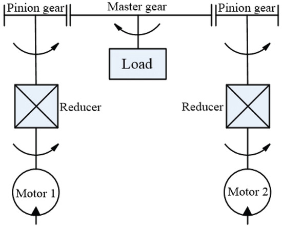
Figure 1.
Structure diagram of the dual-motor drive servo system.
On the basis of [47], ignoring the effects of backlash and actuator fault, this servo system can be modeled as
where and denote the angular position and moment of inertia from load converted to the motor side; indicates the stiffness coefficient of transmission mechanism; , , , and represent the angular position, moment of inertia, electromagnetic torque coefficient, and control signal of two motors; and and stand for the mismatched and matched uncertainties. Assuming that two motors have the same moment of inertia (namely ), setting
and taking
we transform system (1) into
where . As described in [47], the uncertainties and of system (1) may be caused by modeling errors, parameter variations, external disturbances, and so on, which leads to the mismatched uncertainty and its boundary function relying on . In light of this, in order to exploit the general design process of adaptive PTC scheme for UNSs with nontriangular structured uncertain terms, this paper will focus on the following UNSs:
where is the state variable, is the control input, is the output, is an unknown constant vector, is the known virtual control coefficient, is an unknown control gain but its sign is known, and , , and are known nonlinear functions. For , refers to the uncertain term whose strength or magnitude of effect on the system is represented by the positive scalar . To achieve the control objective, we need the following assumptions.
Assumption 1.
For , the uncertain term satisfies
where and are constants; denotes the Euclidean norm.
Remark 1.
Assumption 1 indicates that the boundary of uncertain terms , , relies on all system states, which is also used in [46]. In order to deal with the uncertain term , refs. [25,26,27,28,29,30,31] require that , , or have constant bounds. The condition of is employed in [33,34,35,36,37], where is a triangular structured function. Refs. [38,39,40,41] assume that , where is a constant. In [42,43,44,45], the uncertain term has a pure feedback form, i.e., is associated with . Unlike the aforementioned results, this paper will provide a new idea to cope with the uncertain term that fulfills Assumption 1 and depends on all state variables.
Assumption 2.
For the reference signal , there is a constant such that .
Remark 2.
For the tracking control problem of UNSs, refs. [1,2,3,4,5,6,7,8,9,10,11,12,13,14] need to suppose that the reference signal and its derivatives up to at least the second order are continuously bounded. Meanwhile, Assumption 2 of this paper only requires that the reference signal and its first derivative are continuously bounded. Thus, Assumption 2 in this paper is weaker than that in [1,2,3,4,5,6,7,8,9,10,11,12,13,14] to some extent.
3. Adaptive Practical Tracking Controller Design
In this section, an improved adaptive backstepping technique is adopted to design the state feedback tracking controller and update laws step by step. In the first place, define the error variables
where is the ith stabilizing function to be determined, , for .
Considering the Lyapunov function , according to Assumption 1 and mean square inequality, one can obtain
where , , and are positive constants.
With the selection of the first stabilizing function as
and the use of (6), (8) is changed into
where is a positive constant.
Choosing the Lyapunov function , by applying (10), (11), Assumption 1, and mean square inequality, we have
where and are positive real numbers. Taking the second stabilizing function as
substituting (13) into (12), one yields
where is a positive constant.
Step m (): Assuming that at step , there exists the Lyapunov function such that
where , , , and are positive constants. We will prove that (15) holds at step m.
Taking , by applying (15), (16), Assumption 1, and mean square inequality, it is easy to deduce
where and are positive real numbers.
Selecting the mth stabilizing function as
and substituting (18) into (17), one leads to
which shows that (15) holds at step m, where is a positive constant.
Remark 3.
With the use of (9), one obtains
It is clear that and are constants, so is a linear combination of and . By the same way, one recursively deduces from (6) and (18) that is also a linear combination of , for , i.e.,
where and are constants. It should be emphasized that the linear relationship (20) will play a crucial role in the stability analysis.
Define the parameter estimation errors
where is the estimate of ; denotes the estimate of . Introducing the Lyapunov function
by adopting (19), (21), (22), Assumption 1, and mean square inequality, one can get
where is a positive definite symmetric matrix and and are positive constants.
Choose the state feedback tracking controller
and update laws
where , , and are positive design parameters, is a constant, and is a constant vector. With the help of and
one substitutes (25)–(27) into (24) to achieve
where
Remark 4.
Since in Assumption 2 is bounded and parameters , , , , , and are constants to be designed, it can be seen from (29) that Δ is also bounded, and its boundary can be made as small as possible by adjusting the parameters , , , , , and appropriately.
4. Stability Analysis
We are now in a position to illustrate the first main result of this paper in the following theorem.
Theorem 1.
Supposing that Assumptions 1 and 2 hold for system (5) with nontriangular structured uncertain terms and unknown parameters, under the state feedback tracking controller (25) and update laws (26), if there exists a positive constant such that for , then all signals of the closed-loop system are bounded, and the tracking error finally converges to a bounded interval, that is .
Proof.
Setting
from (6) and (20), it follows that
where , A is an invertible constant matrix, and B is a constant vector.
Applying (31), mean square inequality, and the compatibility of matrix and vector norms, there exists a positive constant such that
where denotes the Frobenius norm.
It can be seen from (20) and (30) that A is related to , which leads to being related to as well, so the positivity of needs to be guaranteed. For , if , we can guarantee that is always positive via suitably selecting parameters .
Defining
for a set of given parameters , denoting
if , it is obvious that . By and the density of real numbers, there must exist such that , which further implies that . Hence, the choice of parameters ensures that .
Letting
it follows from (23) that
where stands for the maximum eigenvalue of . Taking
and using (37), (33) can be rewritten as
According to the comparison principle, integrating (39) over the interval results in
Owing to as and the boundedness of , is ultimately bounded, which implies that , , and are bounded with the help of (23). The boundedness of and u can be established via an induction argument: from (6) and the boundedness of and , we deduce that is bounded. This means that in (9) is bounded, and so is . Using the same manner, (6) and (18), one can recursively prove that and are also bounded for . In view of (25) and the boundedness of , , , , and , it is easy to obtain that u is bounded. Therefore, all signals of the closed-loop system are bounded.
Furthermore, utilizing , if , we deduce from (39) that
which signifies that will decrease until . Hence, we have
This completes the proof. □
Remark 5.
When uncertain terms in [33,34,35,36,37,38,39,40,41] are constrained by the strict feedback form, they can be compensated through adding a bounded function in the stabilizing function at each design step. But in this paper, the boundary of uncertainties is related to all state variables ; then, the traditional adaptive backstepping method is unable to handle it effectively in the first steps. Therefore, mean square inequality is frequently used in each design step to separate and accumulate until the last step. By the feat of (20), we finally establish the linear relationship (31) between state vector ξ and error vector e, which is the key to boundedness analysis.
5. Numerical Examples
This section gives two simulation examples to verify the efficiency of the proposed PTC scheme.
Example 1.
Consider the following UNS
where , , , , and the reference signal . It is easy to show that Assumptions 1 and 2 are satisfied with , , , , and .
Letting and , one gets
Choosing and , (44) becomes
Introducing and using (45), a simple calculation leads to
where and . From (46), we can obtain the improved adaptive tracking controller
Meanwhile, adopting the classic adaptive control technique [16], one also gets
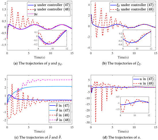
In the simulation, we set unknown parameters ; the design parameters , , , , , ; and the initial values , , . The comparison of simulation results for system (43) under the improved adaptive tracking controller (47) and the classic adaptive tracking controller (48) is offered in Figure 2. Figure 2a presents the system output under controller (47) with a solid line, the system output under controller (48) with a dashed line, and the reference signal with a dotted line. As shown in Figure 2a, it is evident that the system output y under controller (47) tracks the reference signal around 3 s and exhibits relatively few fluctuations with small values, while the system output y under controller (48) tracks the reference signal after 10 s and has frequent fluctuations with large amplitudes. The trajectories of system state , updated laws , , and control input u under controller (47) (see solid line) and controller (48) (see dashed line) are displayed in Figure 2b–d, respectively. One observes from Figure 2b–d that system state, updated laws, and control input under controller (47) also possess a faster response time and smaller fluctuations compared with those under controller (48). Therefore, according to the above comparison, we can conclude that the adaptive PTC approach in Theorem 1 of this paper is superior to [16] in terms of response time and fluctuation degree. Moreover, the control effort required to make the closed-loop system bounded in this paper is also significantly less than that in [16].
Example 2.
To validate the efficiency of the proposed control method in Corollary 1, we simulate the transformed system (4) of the dual-motor drive servo system (1). The system parameters are taken as , , , ; the uncertainties , ; and the reference signal . Choosing , , , , , it is obvious that Assumptions 1 and 2 are fulfilled.
Considering and , one leads to . Taking and , we have
Letting and , by (52), a direct calculation yields
where , , , , . From (53), the robust tracking controller can be chosen as
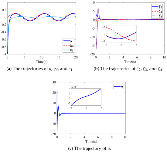
In the simulation, taking the design parameters , , , , and the initial values , , , Figure 3 gives the responses of the closed-loop system (4) and (54) with . The response curves of the system output , the reference signal , and the tracking error are offered in Figure 3a. From Figure 3a, one clearly sees that the system output y (see solid line) is able to track the desired signal (see dashed line) about 2 s later. Meanwhile, the tracking error (see dotted line) is convergent to a bounded region around 2 s. Figure 3b provides the response curves of system states , , and , while Figure 3c depicts the trajectory of control input u. It can be observed from Figure 3b,c that , , , and u are also bounded 2s later. The simulation results in Figure 3 reveal the validity of the control method proposed in Corollary 1.
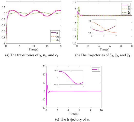
On the other hand, in order to further test the robust property of the control method in Corollary 1, we increase the strength of uncertain terms and in system (4). In this simulation, we set , while keeping all other parameters the same as those in the case where . The simulation results of the closed-loop system (4) and (54) with are shown in Figure 4. By comparing Figure 3 and Figure 4, Figure 4a,b indicate that there is no significant change in the response curves of the system output y and system states , , . However, Figure 4c manifests that after the control input u is bounded, the control effort will increase accordingly due to the increase in the uncertainties’ strength.
6. Conclusions
The adaptive PTC problem for a class of UNSs with nontriangular structured uncertain terms and unknown parameters has been solved in this paper. Different from some existing results on the adaptive PTC of UNSs, this paper utilizes the improved adaptive backstepping technique to construct the adaptive practical tracking controller. With the aid of mean square inequality, the norm of the state vector is separated and accumulated in each design step, which is beneficial for the construction of the implementable controller. Subsequently, by building the linear relationship between the state vector and the error vector and applying the comparison principle, we have certified that the presented adaptive PTC scheme is capable of making the tracking error and other signals of the closed-loop system bounded. Finally, we provide the comparative simulation between the improved adaptive PTC in this paper and the traditional method in [16]. The simulation results illustrate that the controller of this paper has certain advantages in terms of response time and fluctuation degree. Additionally, the simulation of the dual-motor drive servo system further manifests the robustness of the PTC control scheme of this paper.
There still exist some future works: One is to consider the optimal control problem of system (5). Another is to design the suitable online tuning algorithm to determine the design parameters. And the third is to further refine the control scheme of this paper by incorporating the energy management method [48].
Author Contributions
Conceptualization, L.L. and G.S.; methodology, L.L.; software, L.L. and G.S.; validation, L.L., G.S. and R.B.; formal analysis, L.L., G.S. and R.B.; original draft preparation, G.S. and R.B.; review and editing, L.L.; supervision, L.L.; project administration, L.L.; funding acquisition, L.L. All authors have read and agreed to the published version of the manuscript.
Funding
This research was funded by the Young Taishan Scholar Project of Shandong Province of China grant number tsqn202211132, the National Natural Science Foundation of China grant number 61773073 and the Rizhao Natural Science Youth Foundation grant number RZ2024ZR04.
Data Availability Statement
Data is contained within the article.
Conflicts of Interest
The authors declare no conflicts of interest.
References
- Lai, G.Y.; Liu, Z.; Chen, C.L.P.; Zhang, Y. Adaptive asymptotic tracking control of uncertain nonlinear system with input quantization. Syst. Control Lett. 2016, 96, 23–29. [Google Scholar] [CrossRef]
- Xiao, B.; Yang, X.B.; Karimi, H.R.; Qiu, J.B. Asymptotic tracking control for a more representative class of uncertain nonlinear systems with mismatched uncertainties. IEEE Trans. Ind. Electron. 2019, 66, 9417–9427. [Google Scholar] [CrossRef]
- Zhao, X.D.; Wang, X.Y.; Ma, L.; Zong, G.D. Fuzzy approximation based asymptotic tracking control for a class of uncertain switched nonlinear systems. IEEE Trans. Fuzzy Syst. 2020, 28, 632–644. [Google Scholar] [CrossRef]
- Zhao, K.; Song, Y.D.; Chen, C.L.P.; Chen, L. Adaptive asymptotic tracking with global performance for nonlinear systems with unknown control directions. IEEE Trans. Autom. Control 2021, 67, 1566–1573. [Google Scholar] [CrossRef]
- Wu, J.; Sun, W.; Su, S.F.; Wu, Y.Q. Adaptive asymptotic tracking control for input-quantized nonlinear systems with multiple unknown control directions. IEEE Trans. Cybern. 2023, 53, 5216–5225. [Google Scholar] [CrossRef]
- Jia, F.L.; He, X. Active fault-tolerant control with adaptive estimation error compensation for nonlinear systems: Achieving asymptotic tracking. IEEE Trans. Ind. Informat. 2024, 20, 6612–6621. [Google Scholar] [CrossRef]
- Yousef, H. Design of adaptive fuzzy-based tracking control of input time delay nonlinear systems. Nonlinear Dyn. 2015, 79, 417–426. [Google Scholar] [CrossRef]
- Cao, Y.; Cao, J.F.; Song, Y.D. Practical prescribed time tracking control over infinite time interval involving mismatched uncertainties and non-vanishing disturbances. Automatica 2022, 136, 110050. [Google Scholar] [CrossRef]
- Ma, J.W.; Wang, H.Q.; Qiao, J.F. Adaptive neural fixed-time tracking control for high-order nonlinear systems. IEEE Trans. Neural Netw. Learn. Syst. 2022, 35, 708–717. [Google Scholar] [CrossRef]
- Wang, H.Q.; Ai, Z. Adaptive fixed-time tracking control of nonlinear systems with unmodeled dynamics. Nonlinear Dyn. 2024, 112, 21193–21204. [Google Scholar] [CrossRef]
- Liu, Y.C.; Zhu, Q.D. Event-triggered adaptive fuzzy tracking control for uncertain nonlinear systems with time-delay and state constraints. Circuits, Syst. Signal Process. 2022, 41, 636–660. [Google Scholar] [CrossRef]
- Wang, Y.D.; Zong, G.D. Dynamic event-triggered adaptive fixed-time practical tracking control for nonlinear systems through funnel function. IEEE Trans. Autom. Sci. Eng. 2025, 22, 7008–7017. [Google Scholar] [CrossRef]
- Ma, H.; Zhou, Q.; Li, H.Y.; Lu, R.Q. Adaptive prescribed performance control of a flexible-joint robotic manipulator with dynamic uncertainties. IEEE Trans. Cybern. 2022, 52, 12905–12915. [Google Scholar] [CrossRef]
- Lu, K.X.; Han, S.S.; Yang, J.; Yu, H.Y. Inverse optimal adaptive tracking control of robotic manipulators driven by compliant actuators. IEEE Trans. Ind. Electron. 2024, 71, 6139–6149. [Google Scholar] [CrossRef]
- Gheisarnejad, M.; Fathollahi, A.; Sharifzadeh, M.; Laurendeau, E.; Al-Haddad, K. Data-driven switching control technique based on deep reinforcement learning for packed E-cell as smart EV charger. IEEE Trans. Transp. Electrif. 2025, 11, 3194–3203. [Google Scholar] [CrossRef]
- Krstic, M.; Kanellakopoulos, I.; Kokotovic, P.V. Nonlinear and Adaptive Control Design; John Wiley & Sons: New York, NY, USA, 1995. [Google Scholar]
- Zhou, J.; Wen, C.Y.; Wang, W. Adaptive control of uncertain nonlinear systems with quantized input signal. Automatica 2018, 95, 152–162. [Google Scholar] [CrossRef]
- Aslmostafa, E.; Ghaemi, S.; Badamchizadeh, M.A.; Ghiasi, A.R. Adaptive backstepping quantized control for a class of unknown nonlinear systems. ISA Trans. 2022, 125, 146–155. [Google Scholar] [CrossRef]
- Yang, Y.; Huang, J.S.; Su, X.J.; Wang, K.; Li, G.Q. Adaptive control of second-order nonlinear systems with injection and deception attacks. IEEE Trans. Syst. Man, Cybern. Syst. 2022, 52, 574–581. [Google Scholar] [CrossRef]
- Fang, H.Y.; Zhang, M.G.; He, S.P.; Luan, X.L.; Liu, F.; Ding, Z.T. Solving the zero-sum control problem for tidal turbine system: An online reinforcement learning approach. IEEE Trans. Cybern. 2023, 53, 7635–7647. [Google Scholar] [CrossRef]
- Li, Y.M.; Tong, S.C. Adaptive backstepping control for uncertain nonlinear strict-feedback systems with full state triggering. Automatica 2024, 163, 111574. [Google Scholar] [CrossRef]
- Liu, X.P.; Li, N.; Liu, C.G.; Fu, J.; Wang, H.Q. Parameter tuning of modified adaptive backstepping controller for strict-feedback nonlinear systems. Automatica 2024, 166, 111726. [Google Scholar] [CrossRef]
- Hu, L.Y.; Duan, G.R.; Hou, M.Z. Adaptive guaranteed cost control for nonlinear systems with unknown parameters and time delays based on fully actuated system approaches. ISA Trans. 2024, 145, 112–123. [Google Scholar] [CrossRef] [PubMed]
- Hou, Y.X.; Li, S. Event-triggered bipartite formation control for switched nonlinear multi-agent systems with function constraints on states. Actuators 2025, 14, 23. [Google Scholar] [CrossRef]
- Deng, W.X.; Yao, J.Y.; Ma, D.W. Time-varying input delay compensation for nonlinear systems with additive disturbance: An output feedback approach. Int. J. Robust Nonlinear Control 2018, 28, 31–52. [Google Scholar] [CrossRef]
- Fu, L.L.; Ma, R.C.; Pang, H.Z.; Fu, J. Predefined-time tracking of nonlinear strict-feedback systems with time-varying output constraints. J. Frankl. Inst. 2022, 359, 3492–3516. [Google Scholar] [CrossRef]
- Vu, V.T.; Tran, Q.H.; Pham, T.L.; Dao, P.A. Online actor-critic reinforcement learning control for uncertain surface vessel systems with external disturbances. Int. J. Control. Autom. Syst. 2022, 20, 1029–1040. [Google Scholar] [CrossRef]
- Yang, G.C. Asymptotic tracking with novel integral robust schemes for mismatched uncertain nonlinear systems. Int. J. Robust Nonlinear Control 2023, 33, 1988–2002. [Google Scholar] [CrossRef]
- Ma, L.; Gao, Y.F.; Li, B. Distributed fixed-time formation tracking control for the multi-agent system and an application in wheeled mobile robots. Actuators 2024, 13, 68. [Google Scholar] [CrossRef]
- Zheng, X.L.; Yu, X.H.; Yang, X.B.; Zheng, W.X. Adaptive NN zeta-backstepping control with its application to a quadrotor hover. IEEE Trans. Circuits Syst. II Exp. Briefs 2024, 71, 747–751. [Google Scholar] [CrossRef]
- Zhang, Y.; Dai, J.; Liu, Z.; Tang, R.; Zheng, G.; Wang, J. Fixed-time adaptive event-triggered control for uncertain nonlinear systems under full-state constraints. Actuators 2025, 14, 231. [Google Scholar] [CrossRef]
- Fang, H.Y.; He, S.P.; Liu, F.; Ding, Z.T. Policy iterative-based adaptive optimal control for unknown continuous-time nonlinear systems. IEEE Trans. Syst. Man Cybern. Syst. 2025, 55, 2859–2869. [Google Scholar] [CrossRef]
- Jiang, Z.P.; Praly, L. Design of robust adaptive controllers for nonlinear systems with dynamic uncertainties. Automatica 1998, 34, 825–840. [Google Scholar] [CrossRef]
- Wang, H.Q.; Xu, K.; Zhang, H.G. Adaptive finite-time tracking control of nonlinear systems with dynamics uncertainties. IEEE Trans. Autom. Control 2023, 68, 5737–5744. [Google Scholar] [CrossRef]
- Meng, Q.T.; Ma, Q.; Shi, Y. Adaptive fixed-time stabilization for a class of uncertain nonlinear systems. IEEE Trans. Autom. Control 2023, 68, 6929–6936. [Google Scholar] [CrossRef]
- Wu, J.; Yang, Y.D. Neuroadaptive regulation for uncertain systems with quantized states and sensor faults. IEEE Trans. Circuits Syst. II Exp. Briefs 2022, 69, 3199–3203. [Google Scholar] [CrossRef]
- Zhang, W.T.; Yu, B. Adaptive predefined time control for strict-feedback systems with actuator quantization. Actuators 2024, 13, 366. [Google Scholar] [CrossRef]
- Yang, G.C.; Yao, J.Y.; Ullah, N. Neuroadaptive control of saturated nonlinear systems with disturbance compensation. ISA Trans. 2022, 122, 49–62. [Google Scholar] [CrossRef]
- Yang, G.C.; Yao, J.Y.; Dong, Z.L. Neuroadaptive learning algorithm for constrained nonlinear systems with disturbance rejection. Int. J. Robust Nonlinear Control 2022, 32, 6127–6147. [Google Scholar] [CrossRef]
- Ran, M.P.; Li, J.C.; Xie, L.H. Reinforcement-learning-based disturbance rejection control for uncertain nonlinear systems. IEEE Trans. Cybern. 2022, 52, 9621–9633. [Google Scholar] [CrossRef]
- Chen, L.; Dong, C.; Dai, S.L. Adaptive optimal consensus control of multiagent systems with unknown dynamics and disturbances via reinforcement learning. IEEE Trans. Artif. Intell. 2024, 5, 2193–2203. [Google Scholar] [CrossRef]
- Li, Y.M.; Tong, S.C. Adaptive fuzzy output-feedback control of pure-feedback uncertain nonlinear systems with unknown dead zone. IEEE Trans. Fuzzy Syst. 2013, 22, 1341–1347. [Google Scholar] [CrossRef]
- Guo, C.Q.; Hu, J.P.; Wu, Y.Z.; Celikovsky, S. Non-singular fixed-time tracking control of uncertain nonlinear pure-feedback systems with practical state constraints. IEEE Trans. Circuits Syst. I Reg. Papers 2023, 70, 3746–3757. [Google Scholar] [CrossRef]
- Huang, X.C.; Wen, C.Y.; Song, Y.D.; Celikovsky, S. Adaptive neural control for uncertain constrained pure feedback systems with severe sensor faults: A complexity reduced approach. Automatica 2023, 147, 110701. [Google Scholar] [CrossRef]
- Lu, X.Y.; Wang, F. Predefined-time adaptive fuzzy control of pure-feedback nonlinear systems under input and output quantization. Nonlinear Dyn. 2024, 112, 18219–18234. [Google Scholar] [CrossRef]
- Cai, J.P.; Wen, C.Y.; Su, H.Y.; Liu, Z.T.; Xing, L.T. Adaptive backstepping control for a class of nonlinear systems with non-triangular structural uncertainties. IEEE Trans. Autom. Control 2017, 62, 5220–5226. [Google Scholar] [CrossRef]
- Chen, W.; Wu, Y.F.; Du, R.H.; Wu, X.B. Fault diagnosis and fault tolerant control for the servo system driven by two motors synchronously. Control Theory Appl. 2014, 31, 27–34. [Google Scholar]
- Gheisarnejad, M.; Fathollahi, A.; Sharifzadeh, M.; Laurendeau, E.; Andresen, B.; Al-Haddad, K. Optimal policy gradient based type-2 fuzzy control for multi-DC terminal PEC converter in 5G-based commercial buildings. IEEE J. Emerg. Sel. Top. Power Electron. 2025. [Google Scholar] [CrossRef]
Disclaimer/Publisher’s Note: The statements, opinions and data contained in all publications are solely those of the individual author(s) and contributor(s) and not of MDPI and/or the editor(s). MDPI and/or the editor(s) disclaim responsibility for any injury to people or property resulting from any ideas, methods, instructions or products referred to in the content. |
© 2025 by the authors. Licensee MDPI, Basel, Switzerland. This article is an open access article distributed under the terms and conditions of the Creative Commons Attribution (CC BY) license (https://creativecommons.org/licenses/by/4.0/).