Reliable Neural Network Control for Active Vibration Suppression of Uncertain Structures

Abstract

This paper proposes a novel reliable neural network control (NNC) method for active vibration control of uncertain structures. First, reliable model predictive control (MPC) was established by introducing nonprobabilistic reliability constraints into traditional MPC. An importance sampling strategy was established to improve the efficiency of the entire training process to achieve sufficient accuracy. An adaptive nonprobabilistic Kalman filter was further proposed for estimating the uncertain region of system states. Compared to existing reliability-based control methods, the proposed reliable NNC ensured structural safety across broader loads. Compared with reliable MPC, reliable NNC significantly reduced the online computational load, making it suitable for vibration control of high-frequency complex structural systems. The effectiveness and superiority of the proposed reliable NNC were validated through two numerical examples and experimental verification.

1. Introduction

Excessive structural vibrations can cause structural degradation, performance issues, and safety risks, making vibration control crucial for structural integrity. These control methods are mainly divided into passive, semi-active, and active types. With its ability to effectively counteract low-frequency vibrations and high adaptability, active control has become a favored option for improving the performance of complex mechanical systems [1,2].

Uncertainties have a profound impact on the control performance of active vibration control systems. They may even cause system instability and structural damage. In the field of control, robust control is mainly employed to tackle this problem, including $H_{\infty }$ control [3,4], $\mu$-synthesis [5,6], minmax control [7,8], and sliding mode control [9,10], etc. Minmax control is a robust control approach that designs controllers to minimize the worst-case system performance under uncertainties and disturbances, and $H_{\infty }$ control can be regarded as a special case of minmax control. Sliding mode control forces a system to follow a predefined sliding surface, making it insensitive to bounded uncertainties and disturbances via high-frequency switching control inputs. Adaptive control [11,12] is another approach to handle uncertainty, which autonomously adjusts controller parameters in real time to maintain desired performance despite unknown or changing system dynamics. Learning-based control has recently achieved rapid progress, being particularly suited to data-rich but mechanism-complex scenarios. Iterative learning control [13,14] excels in repetitive tasks by optimizing trajectory tracking accuracy through cycle-wise learning, while reinforcement learning control [15,16] demonstrates unique advantages in complex unknown model scenarios. The above uncertain control methods mainly focus on how to reduce the impact of uncertainties on system performance. In the field of structural design, reliability-based optimal design is a type of design method that quantitatively analyzes uncertainties. This concept has also been applied to the design of active controllers for structural vibration. Crespo and Kenny [17] utilized a probabilistic approach and combined it with the first passage rate theory to establish a set of stochastic reliability design methods for active control systems. Li and Wang first established the nonprobabilistic reliability index of the control system, and proposed a reliability-based state feedback control method for structural vibration active control [18]. Yang et al. [19] proposed a reliability-based positioning accuracy index for the design of controllers for industrial robots. However, these methods are all designed for the given external load conditions.

Model predictive control (MPC) is a class of model-based control algorithms. Different from conventional control methods, MPC utilizes the system model to predict the future dynamic behavior of the system [20]. MPC determines the optimal control input sequence by solving an online optimization problem at each time step, aiming to minimize a cost function while satisfying system constraints. The key advantage of MPC lies in its ability to effectively handle complex systems with nonlinearities and constraints, making it particularly well-suited to problems involving hard physical constraints. Considering their ability to withstand the effects of uncertainties, various robust MPC approaches have been proposed and developed. These include nominal model-based robust MPC [21,22], minmax MPC [23,24], tube-based robust MPC [25,26,27], and stochastic MPC [28,29]. Nominal model-based robust MPC tightens constraints to handle uncertainties, offering low-cost computation but excessive conservatism. Minmax MPC addresses the control problem by minimizing the worst-case outcome, treating additive uncertainties as interval parameters. Tube-based robust MPC, conversely, uses robust optimization to determine control actions that keep system trajectories within a specified tube under uncertainties. This approach outperforms minmax MPC, offering less conservatism and lower computational complexity [30]. Dai et al. [31] proposed a tube-based robust MPC for manipulator positioning under additive disturbance.

At present, there have been some studies on the application of MPC in active vibration control. Chen et al. [32] proposed a fast MPC method for structural vibration control based on the unreduced structural finite element model. Wang et al. [33] proposed a distributed adaptive MPC method for active vibration suppression during the assembly process of large-scale space structures. Dubay et al. [34] established a dynamic model via the finite element method and applied MPC to suppress vibrations in a single-joint flexible manipulator, noting its suitability for space structures with low vibration frequencies. However, the online optimization of MPC poses high requirements on the computing power of the controller hardware, which limits its application in structural vibration control. One way to reduce the online computation burden is to pre-calculate the control law offline. For a linear system with a quadratic cost function, the control law can be expressed in the form of a piecewise affine function, which is known as explicit MPC [35]. Explicit MPC reduces the online computation task in solving optimization problems to determine the polytopic region which the system state belongs. Takács et al. [36,37] applied explicit MPC to the active control of structural vibrations and conducted research on issues such as computational efficiency and memory usage in practical control systems. However, the number of polytopic regions of the explicit MPC control law will increase rapidly with the number of constraints, making it difficult for explicit MPC to be applied to the vibration control of complex structural systems. To address the issue of an excessive number of polytopic regions when explicit MPC is applied to complex systems, some researchers have attempted to simplify the control law by eliminating redundant regions. Another category of methods involves approximating the exact solution of MPC. These methods include suboptimal polytope partitioning [38], neural networks [39,40,41], lattice representation [42], and radial basis functions [43]. With the rapid development of the field of machine learning, the method of directly learning the MPC feedback law through neural networks has become very promising. Hertneck et al. [44] proposed a supervised learning framework for approximating the robust MPC feedback law, which offers guarantees on stability and satisfaction of constraints. Gómez et al. [41] enhanced the learning of specific regions in the imitation learning of MPC through importance weighting. Li et al. [45] proposed a novel ‘‘optimize and train’’ method to approximate nonlinear MPC laws.

Existing robust control approaches often face a trade-off between performance conservatism and control effort, sometimes leading to overly restrictive design constraints or practical implementation difficulties. To ensure robustness, they might trade off optimal performance under nominal conditions, resulting in suboptimal operation when uncertainties are minimal. Moreover, existing robust MPC methods fail to characterize uncertainties in detail, causing control strategies to be overly conservative. Additionally, the heavy online computational load of robust MPC conflicts with the high sampling rate needs of vibration control systems. To address the above problems, this paper proposes a reliable neural network control (NNC) method for structural vibration control with hard constraints. Here, “reliable” means that the reliable NNC ensures structural safety through a structural reliability assessment. Firstly, the reliable MPC is established based on the nonprobabilistic reliability theory, and then a reliable NNC law is established through the supervised learning of the reliable MPC law. An overview of the proposed reliable NNC is shown in Figure 1.

The main contributions of the study are summarized as follows:

• This study presents a reliable MPC approach, which is then approximated by neural networks to establish a reliable NNC. In contrast to existing robust MPC methods, the proposed reliable NNC not only ensures the satisfaction of structural reliability constraints but also significantly reduces the online computational burden, making it more practical for real-time control applications.
• A novel importance sampling strategy is introduced. By leveraging an auxiliary neural network to guide the selection of training samples, this strategy effectively enhances the efficiency of the entire training process to achieve sufficient accuracy. This leads to faster convergence during the training process and better generalization ability of the neural network controller.
• An adaptive nonprobabilistic Kalman filter (ANKF) is proposed. Through the use of acceleration data to set adaptive parameters, the ANKF can accurately estimate the system state variables and delineate their uncertain regions in the presence of external disturbance loads. This method provides a more precise and reliable state estimation solution for systems with nonprobabilistic uncertainties.

The subsequent sections of this paper are structured as follows: In Section 2, the dynamic equations of the structural system with nonprobabilistic uncertainties are established. In Section 3, the framework of reliable NNC is introduced along with the establishment of importance sampling strategy. In Section 4, the ANKF is proposed for the estimation of the system states and their error region. Section 5 presents 2 numerical examples and an experimental validation to demonstrate the practicability and effectiveness of the proposed method, with conclusion provided thereafter.

2. Dynamic Model of Smart Structures with Nonprobabilistic Uncertainties and Time Delay

The dynamic equation of a linear structural system under active control and disturbance can be expressed as:

$$M\ddot{z}\left(t\right)+C\dot{z}\left(t\right)+Kz\left(t\right)=P\left(t\right)+L_{u}u\left(t\right)$$

(1)

where $M$, $C$, and $K$ are the mass, damping, and stiffness matrices, respectively. These matrices are all of dimension $n_{DOF}\times n_{DOF}$, where $n_{DOF}$ denotes degrees of freedom (DOFs) of the structural system. $\ddot{z}\left(t\right)$, $\dot{z}\left(t\right)$ and $\ddot{z}\left(t\right)$ denote $n_{DOF}\times 1$ vector of acceleration, velocity, and displacement; $P\left(t\right)$ is the $n_{DOF}\times 1$ disturbance force vector; $u\left(t\right)$ is $n_{control}\times 1$ control input vector, and $n_{control}$ is the number of control inputs. $L_u$ is the $n_{DOF}\times n_{control}$ weighing matrix of control inputs.

Then, the uncertainties of the structural system are incorporated. In this paper, the ellipsoidal model is employed to describe the correlated uncertain variables, which is suitable for situations where it is difficult to obtain sufficient samples of uncertain variables [46]. Assume that there are $n$ uncertain variables and they are be formulated as a vector: $\alpha ={\left[{\alpha }_1,{\alpha }_2,\cdots ,{\alpha }_n\right]}^{\mathrm{T}}$. The uncertain domain of $\alpha$ can be expressed as [47]:

$${\left(\alpha -{\alpha }^c\right)}^{\mathrm{T}}CO{V}_N^{-1}\left(\alpha ,\alpha \right)\left(\alpha -{\alpha }^c\right)\le 1$$

(2)

where $CO{V}_N\left(\cdot ,\cdot \right)$ means the nonprobabilistic auto-covariance matrix, with the subscript $N$ indicating that it is defined within the nonprobabilistic framework; ${\alpha }^c={\left[{\alpha }_1^c,{\alpha }_2^c,\cdots ,{\alpha }_n^c\right]}^{\mathrm{T}}$ is the center point vector. After introducing the uncertainties of the structural system, the dynamic equation of Equation (1) can be rewritten as:

$$M\left(\alpha \right)\ddot{\mathit{z}}\left(t\right)+C\left(\alpha \right)\dot{z}\left(t\right)+K\left(\alpha \right)z\left(t\right)=P\left(t\right)+L_u\left(\alpha \right)u\left(t\right)$$

(3)

In practical engineering applications, the degree of freedom (DOF) of Equation (3) is excessively high, rendering it infeasible for the online computation of MPC. To address this, modal truncation is employed to reduce the DOF. The displacement vector is approximated using the first $n_m$ modes as follows:

$$\ddot{z}\left(t\right)\approx \phi \left(\alpha \right)q={\displaystyle \sum _{i=1}^{n_m}{\phi }_i\left(\alpha \right)q_i\left(t\right)}$$

(4)

where $q\left(t\right)={\left[q_1\left(t\right),\cdots ,q_{n_m}\left(t\right)\right]}^{\mathrm{T}}$ and $\phi \left(\alpha \right)=\left[{\phi }_1\left(\alpha \right),\cdots ,{\phi }_{n_m}\left(\alpha \right)\right]$ are the modal displacement vector and the modal shape matrix, respectively. The modal shape matrix varies with $\alpha$. Modal truncation discards high-frequency modes, making it only suitable for mid-to-low frequency vibration analysis. The dimension of $\phi \left(\alpha \right)$ is $n_{DOF}\times n_m$. Substituting Equation (4) into Equation (3) with left multiplying ${\phi }^{\mathrm{T}}$, we have:

$$\ddot{q}\left(t\right)+2\xi \left(\alpha \right)\omega \left(\alpha \right)\dot{q}\left(t\right)+{\omega }^2\left(\alpha \right)q\left(t\right)={\phi }^{\mathrm{T}}\left(\alpha \right)P\left(t\right)+{\phi }^{\mathrm{T}}\left(\alpha \right)L_u\left(\alpha \right)u\left(t\right)$$

(5)

where

$$\omega \left(\alpha \right)=diag\left\{{\omega }_1,\cdots ,{\omega }_{n_m}\right\},{\omega }_i={\displaystyle \frac{{\phi }_i^{\mathrm{T}}\left(\alpha \right)K\left(\alpha \right){\phi }_i\left(\alpha \right)}{{\phi }_i^{\mathrm{T}}\left(\alpha \right)M\left(\alpha \right){\phi }_i\left(\alpha \right)}},i=1,\cdots ,n_m$$

(6)

and

$$\xi \left(\alpha \right)=diag\left\{{\xi }_1,\cdots ,{\xi }_{n_m}\right\},{\xi }_i={\displaystyle \frac{{\phi }_i^{\mathrm{T}}\left(\alpha \right)C\left(\alpha \right){\phi }_i\left(\alpha \right)}{{\phi }_i^{\mathrm{T}}\left(\alpha \right)M\left(\alpha \right){\phi }_i\left(\alpha \right)}},i=1,\cdots ,n_m$$

(7)

According to the standard form of the state space equation, the state vector is defined as:

$$x\left(t\right)={\left[q^{\mathrm{T}}\left(t\right),{\dot{q}}^{\mathrm{T}}\left(t\right)\right]}^{\mathrm{T}}$$

(8)

and the reduced state space equation with ellipsoidal uncertainties is obtained:

$$\dot{x}\left(t\right)=A\left(\alpha \right)x\left(t\right)+B_F\left(\alpha \right)P\left(t\right)+B_u\left(\alpha \right)u\left(t\right)$$

(9)

where

$$A\left(\alpha \right)=\left[\begin{array}{cc}0& I\\ -{\omega }^2\left(\alpha \right)& 2\xi \left(\alpha \right)\omega \left(\alpha \right)\end{array}\right],B_F\left(\alpha \right)=\left[\begin{array}{c}0\\ {\phi }^{\mathrm{T}}\left(\alpha \right)\end{array}\right],B_u\left(\alpha \right)=\left[\begin{array}{c}0\\ {\phi }^{\mathrm{T}}\left(\alpha \right)L_u\end{array}\right]$$

(10)

and $I$ is the identity matrix.

The system is discretized with fixed sampling interval $\mathrm{\Delta }t$ and the discretized state space equation is written as:

$$x\left(k+1\right)=A^z\left(\alpha \right)x\left(k\right)+B_P^z\left(\alpha \right)P\left(k\right)+B_u^z\left(\alpha \right)u\left(k\right)$$

(11)

where the superscript $z$ indicates that the discrete state equations are obtained by the zero-order hold method. For active control of structural vibration, the time-delay effect of the control system cannot be ignored [48]. This paper considers a case where the time delay is a fixed value and an integer multiple of the time step. Defining the total time delay as $\tau =l\mathrm{\Delta }t$, the discrete state space equation with time delay is expressed as:

$$x\left(k+1\right)=A^z\left(\alpha \right)x\left(k\right)+B_P^z\left(\alpha \right)P\left(k\right)+B_u^z\left(\alpha \right)u\left(k-l\right)$$

(12)

3. The Framework of Reliable NNC

3.1. Establishing Reliable MPC

MPC is a type of control method that solves the optimal control problem within a finite time domain at each sampling instant. To handle systems with time delay using MPC, first, the state equation is transformed into a form without explicit time delay by using the augmented state vector method. Define the augmented state vector as

$$\overline{x}\left(k\right)={\left[x^{\mathrm{T}}\left(k\right),u^{\mathrm{T}}\left(k-l\right),u^{\mathrm{T}}\left(k-l+1\right),\cdots ,u^{\mathrm{T}}\left(k-1\right)\right]}^{\mathrm{T}}$$

(13)

where $u_i^{\mathrm{T}}\left(k\right)=\left[u_i\left(k-l\right),u_i\left(k-l+1\right),\cdots u_i\left(k-1\right)\right]$ and the subscript $i$ represents the serial number of the actuator. Substituting Equation (13) into Equation (12), the state equation of the augmented state vector is obtained as:

$$\overline{x}\left(k+1\right)={\overline{A}}^z\left(\alpha \right)\overline{x}\left(k\right)+{\overline{B}}_P^z\left(\alpha \right)P\left(k\right)+{\overline{B}}_{\phi }^z\left(\alpha \right)u\left(k\right)$$

(14)

where

$${\overline{A}}^z\left(\alpha \right)=\left[\begin{array}{ccccc}{A}^z\left(\alpha \right)& B_{\phi }^z\left(\alpha \right)& 0& \cdots & 0\\ 0& 0& I& \cdots & 0\\ ⋮& ⋮& ⋮& \ddots & ⋮\\ 0& 0& 0& \cdots & I\\ 0& 0& 0& \cdots & 0\end{array}\right],{\overline{B}}_P^z\left(\alpha \right)=\left[\begin{array}{c}{B}_P^z\left(\alpha \right)\\ 0\\ ⋮\\ 0\end{array}\right]{\overline{B}}_{\phi }^z\left(\alpha \right)=\left[\begin{array}{c}0\\ ⋮\\ 0\\ I\end{array}\right]$$

(15)

After obtaining the state equation that does not explicitly contain the time delay, the MPC method can be used to control the system with time delay. The fundamental MPC is established based on the nominal model of the structural system, which will be referred to as nominal MPC in the following text. However, nominal MPC cannot ensure constraint satisfaction when the real system deviates from the nominal system. Therefore, the reliable MPC is established by introducing reliability constraints. Here, the nonprobabilistic reliability theory is utilized to assess the structural system’s reliability, aligning with the ellipsoidal model presented in Section 2. The structural response of interest is denoted as $r\left(x_0,\alpha ,u,P,t\right)$, which is a function of initial conditions $x_0$, uncertain variable vector $\alpha$, control inputs $u$, external loads $P$, and time. The limit state function is constructed so that the concerned response $r\left(x_0,\alpha ,u,P,t\right)$ is not allowed to exceed the critical value $r^{cr}$:

$$g\left(x_0,\alpha ,u,P,t\right)=r^{cr}-r\left(x_0,\alpha ,u,P,t\right)$$

(16)

where $g<0$ means structural failure. The nonprobabilistic time-dependent reliability index is defined as:

$$R_N\left(T\right)=\mathrm{Pos}\left\{\forall t\le T,g\left(x_0,\alpha ,u,P,t\right)\ge 0\right\}$$

(17)

where $\mathrm{Pos}\left\{\cdot \right\}$ is the possibility operation. The nonprobabilistic time-varying reliability index $R_N\left(T\right)$ evaluates the structural safety under the influence of uncertainties. Taking the condition that $R_N\left(T\right)$ is not less than the required value as the constraint, the optimization formulation of reliable MPC at the kth time step is expressed as:

$$\begin{array}{l}\underset{\left\{u_{i\left|k\right.}\right\}}{\min } V_N\left({\overline{x}}^I\left(k\right),u_{i\left|k\right.}\right)\\ \mathrm{s.t.}\hspace{1em}\forall i\in {\mathcal{T}}_{\left[0,N-1\right]}:\\ \hspace{1em}\hspace{1em} {\overline{x}}_{i+1\left|k\right.}={\overline{A}}^z\left({\alpha }^c\right)x_{i\left|k\right.}+{\overline{B}}_{\phi }^z\left({\alpha }^c\right)u_{i\left|k\right.}+{\overline{B}}_P^z\left(\alpha \right)P_{i\left|k\right.},\\ \hspace{1em}\hspace{1em} u_{i\left|k\right.}\in \mathbb{U},\\ \hspace{1em}\hspace{1em} P_{i\left|k\right.}\in P^I,\\ \hspace{1em}\hspace{1em} R_N\left(N\mathrm{\Delta }t\right)\ge R_0,\\ \hspace{1em}\hspace{1em} {\overline{x}}_{N\left|k\right.}^I\subseteq S^{tr},\\ \hspace{1em}\hspace{1em} {\overline{x}}_{0\left|k\right.}\subseteq {\overline{x}}^I\left(k\right).\end{array}$$

(18)

where ${\overline{x}}_{\cdot \left|k\right.}$, $P_{i\left|k\right.}$, and $u_{\cdot \left|k\right.}$ represent the augmented state vector, disturbance load vector, and control input vector after the kth time step, respectively. $x^I\left(k\right)$ is the uncertain interval of the system state at kth time step and $P^I$ is the uncertain interval process of disturbance load. $N$ is the prediction horizon, $\mathbb{U}$ is the feasible set of control input vectors, $R_N\left(N\right)$ is the nonprobabilistic time-dependent reliability index during the time period $\left[0,N\mathrm{\Delta }t\right]$, $R_0$ is the required nonprobabilistic reliability, $S^{tr}$ is the terminal reliable set that ensures the satisfaction of the reliability constraint beyond the prediction horizon, and $V_N$ is the cost function defined in the following quadric form:

$$V_N={\displaystyle \sum _{i=0}^{N-1}\left(x_{i\left|k\right.}^{T}Q{x}_{i\left|k\right.}+u_{i\left|k\right.}^{T}R{u}_{i\left|k\right.}\right)}+x_{N\left|k\right.}^T{Q}_N{x}_{N\left|k\right.}$$

(19)

where $Q$, $R$, and $Q_N$ are the cost weight matrices penalizing state, control input, and final state.

By solving the optimization problem in Equation (18), the control input corresponding to a certain system state can be obtained. It worth noting that the optimization problem in Equation (16) may not always have a feasible solution. This indicates that the current system state exceeds the control capability of the actuator, making it impossible to maintain structural safety. During the optimization process, the nonprobabilistic time-dependent reliability needs to be calculated repeatedly. For the specific process of nonprobabilistic time-dependent reliability analysis, please refer to our previous work [49].

3.2. Approximating Reliable MPC with a Deep Neural Network (DNN)

Due to its strong fitting ability, a DNN is an effective means to approximate the reliable MPC law. The sample set of reliable MPC is obtained by solving the optimization problem in Equation (18), and a deep neural network is trained. Once the training is completed, the neural network can replace the original reliable MPC law. A DNN for control law approximation is defined in the form of the following composite function:

$${\mathcal{N}}_{control}\left(x,\theta \right)={\mu }_{L+1}\circ {\lambda }_L\circ {\mu }_L\circ \cdots \circ {\mu }_0\circ {\lambda }_0\left(x\right)$$

(20)

where $L$ is the number of hidden layers, ${\lambda }_0\left(x\right)=W_{0}x+b_0$ is the affine transformation of the input layer, ${\lambda }_l\left({\xi }_{l-1}\right)=W_l{\xi }_{l-1}+b_l$ is the affine transformation of each hidden layer, and ${\mu }_l\left(\cdot \right)$ is the activation function.

For the structural system with the first $n_m$ order modes retained, the central point vector of the system states contains $2n_m$ variables, and the autocorrelation function contains $2n_m\left(n_m+1\right)$ variables. Then, the total number of input variables of the neural network is $2n_m\left(n_m+2\right)$. A too-large number of input variables will not only lead to a substantial increase in the number of samples required for the training of the surrogate model, but also make the neural network too complex, resulting in too long a time for a single forward calculation. Therefore, a conservative estimate is adopted for the uncertainty of the system state, and the interval model is used to replace the ellipsoidal model. Such treatment will make the modified reliable MPC a bit more conservative, but it can change the input variables to the central value and the radius of the system state, a total of $2n_m+1$ variables, which greatly reduces the difficulty of neural network training.

There inherently exists an error between the neural network output and the direct solution of the reliable MPC. For reliable MPC, this error can be treated as part of the control system’s uncertainty. By incorporating the uncertainty of control variables into the reliable MPC optimization formulation, the reduction in reliability due to neural network errors is mitigated. Based on the consideration above, the original reliable MPC optimization formulation is transformed as follows:

$$\begin{array}{l}\underset{\left\{u_{i\left|k\right.}\right\}}{\min } V_N\left(x\left(k\right),u_{i\left|k\right.}\right)\\ \mathrm{s}.\mathrm{t}. \forall i\in {\mathcal{T}}_{\left[0,N-1\right]}:\\ \hspace{1em} {\overline{x}}_{i+1\left|k\right.}={\overline{A}}^z\left({\alpha }^c\right)x_{i\left|k\right.}+{\overline{B}}_{\phi }^z\left({\alpha }^c\right)\left(u_{i\left|k\right.}+u_{i\left|k\right.}^{\mathrm{uncertain}}\right)+{\overline{B}}_P^z\left(\alpha \right)P_{i\left|k\right.},\\ \hspace{1em} u_{i\left|k\right.}\in \mathbb{U},\\ \hspace{1em} P_{i\left|k\right.}\in P^I,\\ \hspace{1em} R_N\left(N\mathrm{\Delta }t\right)\ge R_0,\\ \hspace{1em} x_{N\left|k\right.}^I\in S^t,\\ \hspace{1em} x_{0\left|k\right.}\in x^I\left(k\right)\\ \hspace{1em} \left|u_{i\left|k\right.}^{\mathrm{uncertain}}\right|<\eta .\end{array}$$

(21)

where $u_{i\left|k\right.}^{\mathrm{uncertain}}$ is the uncertain part of the control input vector.

To train the neural network, first select $N_s$ input samples $x^i$, and solve the corresponding control inputs ${\pi }_{\mathrm{reliable}}\left(x^i\right)$ according to the optimization formulation in Equation (21) to obtain the training sample set:

$$\mathcal{T}=\left[\left(x^1,{\pi }_{\mathrm{reliable}}\left(x^1\right)\right),\cdots ,\left(x^{N_s},{\pi }_{\mathrm{reliable}}\left(x^{N_s}\right)\right)\right]$$

(22)

The mean squared error is selected as the cost function for neural network training. By minimizing the cost function, the optimal parameters of the neural network are obtained:

$${\theta }^{*}=\underset{\theta }{\arg \min }{\displaystyle \frac{1}{N_s}}{\displaystyle \sum _{i=1}^{N_s}{‖{\pi }_{\mathrm{reliable}}\left(x^i\right)-{\mathcal{N}}_{control}\left(x^i,\theta \right)‖}^2}$$

(23)

Ultimately, the reliable NNC law is obtained:

$${\pi }_{\mathrm{RNNC}}\left(x\right)={\mathcal{N}}_{control}\left(x,{\theta }^{*}\right)$$

(24)

3.3. Importance Sampling Strategy

The NNC law obtained through supervised learning demonstrates good performance for the scenarios covered by the training samples. However, its control performance will significantly decline for scenarios that are not covered by the training samples [50]. The most straightforward approach to addressing the above issues is to increase the number of samples to cover as many possible scenarios as possible. Nevertheless, as the number of samples increases, the inefficiency of the method of uniform sampling within the sample space will become more evident. Additionally, uniform sampling will select a large number of points with infeasible solutions, further affecting the efficiency of sample point generation.

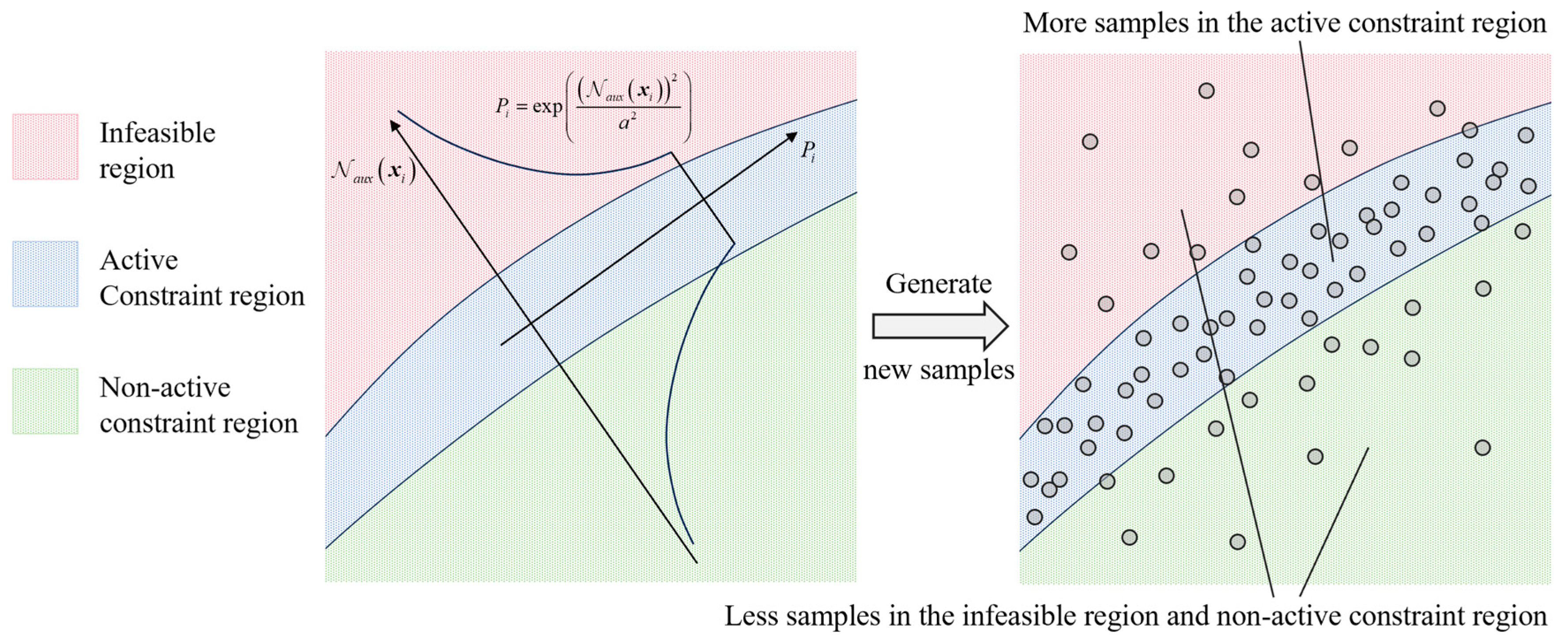
The primary objective of training a DNN is to approximate the reliable model MPC law. The reliable MPC employs the same quadratic cost function as linear quadratic regulator (LQR) control. Consequently, when the online optimization’s reliability constraint is inactive, the reliable MPC law mirrors the linear state feedback characteristics of LQR control, as illustrated in the cyan region of Figure 2. Conversely, activation of the reliability constraint induces pronounced nonlinear behaviors, such as abrupt gradient changes, depicted in the yellow and dark blue regions of Figure 2. These active-constraint regions entail intricate nonlinear mappings, necessitating a larger quantity of sample points for training a neural network capable of accurately capturing these relationships. Evidently, sample points with active reliability constraints are of greater significance for network training compared to those with inactive constraints. Therefore, in this section, an importance sampling strategy is proposed, and an auxiliary neural network for the reliability index is established to guide the selection of sample points.

From the previous analysis, it is desirable to select as many sample points as possible where the reliability constraints are active. However, whether the reliability constraints are active is unknown before solving the problem in Equation (21) for the sample points. In order to determine whether the reliability constraints are effective, an auxiliary neural network ${\mathcal{N}}_{aux}$ is introduced. ${\mathcal{N}}_{aux}$ has a similar structure to ${\mathcal{N}}_{control}$.

The inputs of this auxiliary neural network are the system state and the control quantity at the previous moment, and the output is the value of the reliability constraint function corresponding to the optimal solution. If the value of the reliability constraint function is less than 0, it indicates that the constraint is non-active; if the reliability constraint function is equal to 0, it indicates that the constraint is active; and if it is greater than 0, it means that no feasible solution can be found. By using the reliability constraint function, the discrete problem of determining whether the constraint is active is transformed into the evaluation of a continuous function.

First, generate the initial sample set based on some given load conditions. The outputs of these samples include not only the control variables but also the values of the reliability constraint function corresponding to the optimal solutions. Then, train the auxiliary neural network using the initial sample set.

When adding new sample points, first use the Latin hypercube sampling to obtain a candidate sample set ${\mathcal{T}}_{\mathrm{candidate}}$ .Then, use the auxiliary neural network ${\mathcal{N}}_{aux}$ to evaluate the values of the reliability constraint function for these samples. The output values of the auxiliary neural network corresponding to the sample points where the constraints take effect may not necessarily be equal to 0. For the sample points in the set, randomly decide whether to retain each sample point according to the probability determined by the following Gaussian function:

$$P_i=\exp \left(-{\displaystyle \frac{{\left({\mathcal{N}}_{aux}\left(x_i,{\theta }_{aux}^{*}\right)\right)}^2}{a^2}}\right)$$

(25)

where the parameter $a$ determines the width of the importance sampling and ${\theta }_{aux}^{*}$ is the optimal parameters obtained through training. When the output value of the auxiliary neural network for a sample point is closer to 0, the probability of retaining the sample point is closer to 1. This way of selecting newly added sample points enables the selection of more sample points for which the reliability constraint is active, while also selecting some sample points with non-active constraint, as illustrated in Figure 3. The addition of new samples is carried out in batches. Each time a batch of new samples is selected, the auxiliary neural network is retrained to enhance its accuracy, thereby minimizing the risk of biased sample selection.

After selecting $N_{new}$ sample points, solve the reliable MPC control law for these newly added sample points to obtain an updated sample set, and then retrain the auxiliary neural network. To determine whether a sufficient number of sample points have been selected, the hypersphere coverage index is introduced to characterize whether the existing samples effectively cover the region where the constraints take effect. For each sample point, a hypersphere with the point as the center and a radius of $r$ is defined. The volume of the space where the value of the reliability constraint function lies in the range of $\left[-0.1,0.1\right]$ is defined as $V_{\mathrm{constrained}}$, and the hyper-volume of the region where the value of the reliability constraint function lies in the range of $\left[-0.1,0.1\right]$ and is covered by the hyperspheres of the sample points is defined as $V_{\mathrm{covered}}$. Then, the hypersphere coverage index $I_{hs}$ is defined as:

$$I_{hs}={\displaystyle \frac{V_{\mathrm{covered}}}{V_{\mathrm{constrained}}}}$$

(26)

$I_{hs}$ reflects the density of sample points within the space where the reliability constraint function range is $\left[-0.1,0.1\right]$. Since it is difficult to analytically calculate the hyper-volume, the Monte Carlo method is used here to numerically solve $I_{hs}$, and during the calculation process, the auxiliary neural network is employed to replace the reliability constraint function. If $I_{hs}$ is smaller than the required value, then continue to add new sample points and update the auxiliary neural network using the same method until $I_{hs}$ meets the requirement, and the final sample set is obtained. The control law neural network is trained with the final sample set.

3.4. Procedure for Training the Reliable NNC Law

The procedure of training the reliable NNC law is listed below.

Step 1. Apply the preselected external load to the closed-loop system with the reliable MPC, and conduct a dynamic analysis to obtain the initial sample set ${\mathcal{T}}_{initial}$.

Step 2. Train the auxiliary neural network ${\mathcal{N}}_{aux}$ using the initial sample set ${\mathcal{T}}_{initial}$.

Step 3. Generate the candidate sample set ${\mathcal{T}}_{\mathrm{candidate}}$ using a Latin hypercube sampling technique, and use ${\mathcal{N}}_{aux}$ to evaluate the values of the reliability constraint for the sample points of ${\mathcal{T}}_{initial}$, and set $i=1$.

Step 4. According to the probability determined by Equation (25), judge one by one whether the samples in ${\mathcal{T}}_{\mathrm{candidate}}$ should be added to the $i\mathrm{th}$ new sample set ${\mathcal{T}}_{\mathrm{new}}^i$. When the number of new samples reaches $N_{new}$, the construction of ${\mathcal{T}}_{\mathrm{new}}^i$ is completed.

Step 5. Retrain the auxiliary neural network ${\mathcal{N}}_{aux}$ with the sample set ${\mathcal{T}}_{initial}{\mathcal{T}}_{new}^1\cup \cdots \cup {\mathcal{T}}_{new}^i$, and calculate the space filling index $I_{\mathrm{infill}}$.

Step 6. Judge whether $I_{hs}>0.99$. If yes, jump to Step 7; otherwise, set $i=i+1$ and jump to Step 4.

Step 7. Train the control law network ${\mathcal{N}}_{aux}$ with the sample set ${\mathcal{T}}_{initial}\cup {\mathcal{T}}_{new}^1\cup \cdots \cup {\mathcal{T}}_{new}^i$, and obtain the root mean square error (RMSE) ${\sigma }_{control}$ of ${\mathcal{N}}_{contol}$.

Step 8. Judge whether $3{\sigma }_{control}<\eta$. If yes, end the training process; otherwise, jump to Step 9.

Step 9. If the number of training times is less than $N_{train}$, go back to Step 7 for retraining; if the number of training times reaches $N_{train}$, set $\eta =3{\sigma }_{control,\min }$, where ${\sigma }_{control,\min }$ is the minimum value of the RMSEs in the $N_{train}$ training sessions, and then jump to Step 10.

Step 10. Update the reliable MPC optimization formulation according to the modified $\eta$, recalculate the control input corresponding to the samples in ${\mathcal{T}}_{initial}\cup {\mathcal{T}}_{new}^1\cup \cdots \cup {\mathcal{T}}_{new}^i$, and then return to Step 7 for retraining.

The flowchart of training the reliable NNC law is shown in Figure 4.

4. Adaptive Nonprobabilistic Kalman Filter for State Estimation

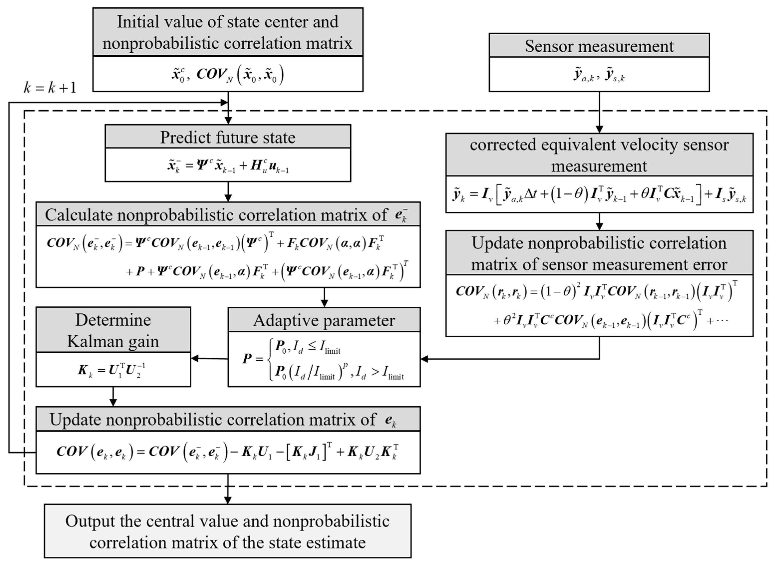
The state variables of a structural system are modal displacements and modal velocities. If the sensor data does not include velocity measurements, the estimated modal velocity under strong external disturbances may require a considerable amount of time to converge near the true values. However, in practical applications, direct measurement of the velocity at a specific point of a structure is generally infeasible. Velocity signals are obtained by integrating acceleration measurements through velocity sensors, which can lead to error accumulation. To address this, an adaptive nonprobabilistic Kalman filter (ANKF) suitable for combined use of accelerometers and strain gauges is developed in this section.

The true values measured by the accelerometers and strain gauges can be expressed as:

$$y_{a,k}=C_a\left(\alpha \right){\dot{x}}_k, y_{s,k}=C_s\left(\alpha \right)x_k$$

(27)

where $C_a\left(\alpha \right)$ and $C_s\left(\alpha \right)$ are matrices that vary with the uncertain variable $\alpha$. Define ${\tilde{y}}_{a,k}$ and ${\tilde{y}}_{s,k}$ as the measured values from the sensors; they can be expressed as:

$${\tilde{y}}_{a,k}=y_{a,k}+w_a, {\tilde{y}}_{s,k}=y_{s,k}+w_s$$

(28)

where $w_a$ and $w_s$ are the measurement noises of the acceleration sensors and the strain sensors, respectively. Since the measured value of the acceleration sensor cannot be directly represented by a linear combination of the state variables, the equivalent velocity sensor that measures the velocity at the measurement point of the acceleration sensor is constructed. The true value of the equivalent velocity sensor measurement is:

$$y_{v,k}=C_a{x}_k$$

(29)

Since the uncertain parameter vector $\alpha$ is bounded, a first-order expansion of the system matrix can be performed:

$$A^z\left(\alpha \right)=A^{z,c}+{\displaystyle \sum _{i=1}^n{A}_i^{z,r}{\alpha }_i},B_u^z\left(\alpha \right)=B_u^{z,c}+{\displaystyle \sum _{i=1}^n{B}_{u,i}^{z,r}{\alpha }_i},C\left(\alpha \right)=C^c+{\displaystyle \sum _{i=1}^n{C}_i^r{\alpha }_i}$$

(30)

where ${\alpha }_i$ is the $i\mathrm{th}$ component of the uncertain variable vector $\alpha$. The prior estimation ${\tilde{x}}_k^{-}$ is the prediction based on the central values of the system matrices, expressed as:

$${\tilde{x}}_k^{-}=A^{z,c}{\tilde{x}}_{k-1}+B_u^{z,c}{u}_{k-l-1}$$

(31)

The posterior estimation ${\tilde{x}}_k$ is obtained by correcting the prior estimation using the sensor measurements:

$${\tilde{x}}_k={\tilde{x}}_k^{-}+K_k\left({\tilde{y}}_k-C^c{\tilde{x}}_k^{-}\right)$$

(32)

where $K_k$ is the Kalman gain. The prior error $e_k^{-}$ and the posterior error $e_k$ are defined as follows:

$$e_k^{-}=x_k-{\tilde{x}}_k, e_k=x_k-{\tilde{x}}_k$$

(33)

Substitute Equation (31) into Equation (33) yield:

$$\begin{array}{l}{e}_k^{-}=\left(\left(A^{z,c}+{\displaystyle \sum _{i=1}^n{A}_i^{z,r}{\alpha }_i}\right)x_{k-1}+\left(B_u^{z,c}+{\displaystyle \sum _{i=1}^n{B}_{u,i}^{z,r}{\alpha }_i}\right)u_{k-1}+p_{k-1}\right)-\left(A^{z,c}{\tilde{x}}_{k-1}+B_u^{z,c}{u}_{k-l-1}\right)\\ \hspace{1em} \approx A^{z,c}{e}_{k-1}+F_k\alpha +p_{k-1}\end{array}$$

(34)

where $F_k=\left[A_1^{z,r}{\tilde{x}}_{k-1}^{-}+B_{u,1}^{z,r}{u}_{k-l-1},A_2^{z,r}{\tilde{x}}_{k-1}^{-}+B_{u,2}^{z,r}{u}_{k-l-1},\cdots ,A_n^r{\tilde{x}}_{k-1}^{-}+B_{u,n}^{z,r}{u}_{k-l-1}\right]$ and the quadratic terms are discarded. Based on the interval process theory [47], the nonprobabilistic autocorrelation matrix of $e_k^{-}$ can be obtained as follows:

$$\begin{array}{l}CO{V}_N\left(e_k^{-},e_k^{-}\right)=A^{z,c}CO{V}_N\left(e_{k-1},e_{k-1}\right){\left({\Psi }^c\right)}^{\mathrm{T}}+F_{k}CO{V}_N\left(\alpha ,\alpha \right)F_k^{\mathrm{T}}\\ \hspace{1em}\hspace{1em}\hspace{1em}\hspace{1em}\hspace{1em}\hspace{1em}+P_N+A^{z,c}CO{V}_N\left(e_{k-1},\alpha \right)F_k^{\mathrm{T}}+{\left(A^{z,c}CO{V}_N\left(e_{k-1},\alpha \right)F_k^{\mathrm{T}}\right)}^T\end{array}$$

(35)

where $P_N$ is the nonprobabilistic autocorrelation matrix of process noise, and it can be seen as a tunable parameter. The signal of the equivalent velocity sensor is obtained by numerically integrating the signal from the acceleration sensor:

$$y_{v,k}=y_{v,k-1}+y_{a,k}\mathrm{\Delta }t$$

(36)

Considering that numerical integration will lead to the divergence of the error, the posterior estimation of the state is used for correction. The vector of sensor measurement values including the equivalent velocity sensor is:

$${\tilde{y}}_k=I_v\left[{\tilde{y}}_{a,k}\mathrm{\Delta }t+\left(1-\theta \right)I_v^{\mathrm{T}}{\tilde{y}}_{k-1}+\theta I_v^{\mathrm{T}}{C}^c{\tilde{x}}_{k-1}\right]+I_s{\tilde{y}}_{s,k}$$

(37)

where $\theta$ is the correction factor, which is a small positive number. The error of the equivalent sensor measurement is:

$$r_k=y_k-{\tilde{y}}_k=I_v\left[-w_a\mathrm{\Delta }t+\left(1-\theta \right)I_v^{\mathrm{T}}{r}_{k-1}+\theta I_v^{\mathrm{T}}\left(C^c{e}_{k-1}+{\displaystyle \sum _{i=1}^n{C}_i^r{\tilde{x}}_{k-1}{\alpha }_i}+{\displaystyle \sum _{i=1}^n{C}_i^r{e}_{k-1}{\alpha }_i}\right)\right]-I_s{w}_s$$

(38)

Omitting the quadratic term ${\displaystyle \sum _{i=1}^n{C}_i^r{e}_{k-1}{\alpha }_i}$, Equation (38) can be approximated as:

$$r_k\approx \left(1-\theta \right)I_v{I}_v^{\mathrm{T}}{r}_{k-1}+\theta I_v{I}_v^{\mathrm{T}}{C}^c{e}_{k-1}+\theta I_v{I}_v^{\mathrm{T}}{L}_{k-1}\alpha -I_v{w}_a\mathrm{\Delta }t-I_s{w}_s$$

(39)

where $L_{k-1}=\left[\begin{array}{cccc}{C}_1^r{\tilde{x}}_{k-1}& C_2^r{\tilde{x}}_{k-1}& \cdots & C_n^r{\tilde{x}}_{k-1}\end{array}\right]$. The nonprobabilistic autocorrelation matrix of $r_k$ can be expressed as:

$$\begin{array}{l}CO{V}_N\left(r_k,r_k\right)={\left(1-\theta \right)}^2{I}_v{I}_v^{\mathrm{T}}CO{V}_N\left(r_{k-1},r_{k-1}\right){\left(I_v{I}_v^{\mathrm{T}}\right)}^{\mathrm{T}}\\ \hspace{1em}\hspace{1em}\hspace{1em}\hspace{1em}\hspace{1em}\hspace{1em} +{\theta }^2{I}_v{I}_v^{\mathrm{T}}{C}^{c}CO{V}_N\left(e_{k-1},e_{k-1}\right){\left(I_v{I}_v^{\mathrm{T}}{C}^c\right)}^{\mathrm{T}}+{\theta }^2{I}_v{I}_v^{\mathrm{T}}{L}_{k-1}CO{V}_N\left(\alpha ,\alpha \right){\left(I_v{I}_v^{\mathrm{T}}{L}_{k-1}\right)}^{\mathrm{T}}\\ \hspace{1em}\hspace{1em}\hspace{1em}\hspace{1em}\hspace{1em}\hspace{1em} +\left(1-\theta \right)\theta I_v{I}_v^{\mathrm{T}}CO{V}_N\left(r_{k-1},e_{k-1}\right){\left(I_v{I}_v^{\mathrm{T}}{C}^c\right)}^{\mathrm{T}}+{\left(\left(1-\theta \right)\theta I_v{I}_v^{\mathrm{T}}CO{V}_N\left(r_{k-1},e_{k-1}\right){\left(I_v{I}_v^{\mathrm{T}}{C}^c\right)}^{\mathrm{T}}\right)}^{\mathrm{T}}\\ \hspace{1em}\hspace{1em}\hspace{1em}\hspace{1em}\hspace{1em}\hspace{1em} +\left(1-\theta \right)\theta I_v{I}_v^{\mathrm{T}}CO{V}_N\left(r_{k-1},\alpha \right){\left(I_v{I}_v^{\mathrm{T}}{L}_{k-1}\right)}^{\mathrm{T}}+{\left(\left(1-\theta \right)\theta I_v{I}_v^{\mathrm{T}}CO{V}_N\left(r_{k-1},\alpha \right){\left(I_v{I}_v^{\mathrm{T}}{L}_{k-1}\right)}^{\mathrm{T}}\right)}^{\mathrm{T}}\\ \hspace{1em}\hspace{1em}\hspace{1em}\hspace{1em}\hspace{1em}\hspace{1em} +{\theta }^2{I}_v{I}_v^{\mathrm{T}}{C}^{c}CO{V}_N\left(e_{k-1},\alpha \right){\left(I_v{I}_v^{\mathrm{T}}{L}_{k-1}\right)}^{\mathrm{T}}+{\left({\theta }^2{I}_v{I}_v^{\mathrm{T}}{C}^{c}CO{V}_N\left(e_{k-1},\alpha \right){\left(I_v{I}_v^{\mathrm{T}}{L}_{k-1}\right)}^{\mathrm{T}}\right)}^{\mathrm{T}}\\ \hspace{1em}\hspace{1em}\hspace{1em}\hspace{1em}\hspace{1em}\hspace{1em}\hspace{1em} +I_v{W}_a{I}_v^{\mathrm{T}}\mathrm{\Delta }{t}^2+I_s{W}_s{I}_s^{\mathrm{T}}\end{array}$$

(40)

It can be seen that in order to obtain $CO{V}_N\left(r_k,r_k\right)$, it is necessary to calculate $CO{V}_N\left(r_{k-1},e_{k-1}\right)$, $CO{V}_N\left(r_{k-1},\alpha \right)$, and $CO{V}_N\left(e_{k-1},\alpha \right)$ in the previous time step. In other words, in order to calculate $CO{V}_N\left(r_{k+1},r_{k+1}\right)$ at the $k+1$ time step, it is necessary to calculate $CO{V}_N\left(r_k,e_k\right)$, $CO{V}_N\left(r_k,\alpha \right)$, and $CO{V}_N\left(e_k,\alpha \right)$ at the $k$ time step. The expression of $CO{V}_N\left(r_k,\alpha \right)$ is derived:

$$CO{V}_N\left(r_k,\alpha \right)=I_v{I}_v^{\mathrm{T}}\left[\left(1-\theta \right)CO{V}_N\left(r_{k-1},\alpha \right)+\theta C^{c}CO{V}_N\left(e_{k-1},\alpha \right)+\theta L_{k-1}CO{V}_N\left(\alpha ,\alpha \right)\right]$$

(41)

To further obtain the correlation matrix related to the posterior error, it is necessary to first derive $e_k$:

$$\begin{array}{l}CO{V}_N\left(e_k^{-},r_k\right)=\left(1-\theta \right)A^{z,c}CO{V}_N\left(e_{k-1},r_{k-1}\right){\left(I_v{I}_v^{\mathrm{T}}\right)}^{\mathrm{T}}+\theta A^{z,c}CO{V}_N\left(e_{k-1},e_{k-1}\right){\left(I_v{I}_v^{\mathrm{T}}{C}^c\right)}^{\mathrm{T}}\\ \hspace{1em}\hspace{1em}\hspace{1em}\hspace{1em}\hspace{1em}\hspace{1em} +\theta A^{z,c}CO{V}_N\left(e_{k-1},\alpha \right){\left(I_v{I}_v^{\mathrm{T}}{L}_{k-1}\right)}^{\mathrm{T}}+\left(1-\theta \right)F_{k}CO{V}_N\left(\alpha ,r_{k-1}\right){\left(I_v{I}_v^{\mathrm{T}}\right)}^{\mathrm{T}}\\ \hspace{1em}\hspace{1em}\hspace{1em}\hspace{1em}\hspace{1em}\hspace{1em} +\theta F_{k}CO{V}_N\left(\alpha ,e_{k-1}\right){\left(I_v{I}_v^{\mathrm{T}}{C}^c\right)}^{\mathrm{T}}+\theta F_{k}CO{V}_N\left(\alpha ,\alpha \right){\left(I_v{I}_v^{\mathrm{T}}{L}_{k-1}\right)}^{\mathrm{T}}\end{array}$$

(42)

$e_k$ can be expressed as:

$$\begin{array}{l}{e}_k=x_k-{\tilde{x}}_k^{-}-K_k\left(y_k-C^c{\tilde{x}}_k^{-}\right)\\ \approx \left(I-K_k{C}^c\right)e_k^{-}+K_k{r}_k-K_k{L}_k^{-}\alpha \end{array}$$

(43)

where $L_k^{-}=\left[\begin{array}{cccc}{C}_1^r{\tilde{x}}_k^{-}& C_2^r{\tilde{x}}_k^{-}& \cdots & C_n^r{\tilde{x}}_k^{-}\end{array}\right]$, and the quadric terms are omitted in Equation (43). The nonprobabilistic autocorrelation matrix of $e_k$ can be expressed as:

$$CO{V}_N\left(e_k,e_k\right)=CO{V}_N\left(e_k^{-},e_k^{-}\right)-K_k{U}_1-{\left[K_k{J}_1\right]}^{\mathrm{T}}+K_k{U}_2{K}_k^{\mathrm{T}}$$

(44)

where

$$U_1=C^c\cdot CO{V}_N\left(e_k^{-},e_k^{-}\right)-CO{V}_N\left(r_k,e_k^{-}\right)+CO{V}_N\left(e_k^{-},\alpha \right){\left(L_k^{-}\right)}^{\mathrm{T}}$$

(45)

and

$$\begin{array}{l}{U}_2=C^c\cdot CO{V}_N\left(e_k^{-},e_k^{-}\right){\left(C^c\right)}^{\mathrm{T}}-C^c\cdot CO{V}_N\left(e_k^{-},r_k\right)-CO{V}_N\left(r_k,e_k^{-}\right){\left(C^c\right)}^{\mathrm{T}}\\ +C^c\cdot CO{V}_N\left(e_k^{-},\alpha \right){\left(L_k^{-}\right)}^{\mathrm{T}}+L_k^{-}CO{V}_N\left(\alpha ,e_k^{-}\right){\left(C^c\right)}^{\mathrm{T}}+CO{V}_N\left(r_k,r_k\right)\\ +L_k^{-}CO{V}_N\left(\alpha ,\alpha \right){\left(L_k^{-}\right)}^{\mathrm{T}}-CO{V}_N\left(r_k,\alpha \right){\left(L_k^{-}\right)}^{\mathrm{T}}-{\left(CO{V}_N\left(r_k,\alpha \right){\left(L_k^{-}\right)}^{\mathrm{T}}\right)}^{\mathrm{T}}\end{array}$$

(46)

The purpose of introducing the Kalman gain $K_k$ is to correct the prior estimation and obtain a posterior estimation with higher accuracy. Therefore, $K_k$ can be determined by minimizing the posterior error $e_k$. The objective function is defined as the trace of $CO{V}_N\left(e_k,e_k\right)$, which represents the sum of the squared interval radius of all posterior error components. The objective function $J$ is expressed as:

$$J=\mathrm{tr}\left(CO{V}_N\left(e_k,e_k\right)\right)$$

(47)

Taking the derivative of $J$ with respect to $K_k$, we obtain:

$${\displaystyle \frac{\partial J}{\partial K_k}}=-2U_1^{\mathrm{T}}+2K_k{U}_2$$

(48)

Minimizing the objective function requires ${\displaystyle \frac{\partial J}{\partial K_k}}=0$, thereby enabling the determination of the Kalman gain as:

$$K_k=U_1^{\mathrm{T}}{U}_2^{-1}$$

(49)

The Kalman filter achieves state estimation by utilizing both the sensor signals and the model-based prediction. Since the external disturbance is unknown, when the external disturbance is significantly large, the model-based prediction will become inaccurate. In such a case, the state estimation should be more inclined to rely on sensor signals. The signals from the acceleration sensor can be used to determine the magnitude of the external disturbance. The acceleration at the measurement points of the accelerometer based on the model prediction is:

$$y_{a,k}^{*}=C_a\left(A_c{\tilde{x}}_k+B_c{u}_k\right)$$

(50)

The deviation between the predicted acceleration and the measured acceleration from the sensor can reflect the magnitude of the external disturbance, and a disturbance index is defined:

$$I_d={‖y_{a,k}-y_{a,k}^{*}‖}_2$$

(51)

When $I_d$ exceeds a predefined threshold $I_{\mathrm{limit}}$, increase the Kalman parameter $P_N$ to prioritize sensor measurements in the state estimation.

$$P_N=\left\{\begin{array}{l}{P}_0,I_d\le I_{\mathrm{limit}}\\ P_0{\left(I_d/I_{\mathrm{limit}}\right)}^p, I_d>I_{\mathrm{limit}}\end{array}\right.$$

(52)

The operation process of the ANKF is shown in Figure 5.

5. Numerical Examples and Experimental Validation

Two numerical cases and an experimental validation are utilized to show the application of the proposed method. For the numerical example and the experimental validation, both the reliable MPC and reliable NNC were implemented on a laptop with a i5-9300H CPU, 16 GB RAM, and NVIDIA GeForce GTX 1660 Ti.

5.1. Numerical Example 1: Cantilever Beam

In this numerical example, a cantilever beam with active control was used, as shown in Figure 6. The cantilever beam was made of aluminum alloy and had a uniform cross-section. Two macro fiber composite (MFC) [51] patches were bonded to the surface of the beam as actuators. Control inputs were the voltages of the MFC patches and the unit was V. Two displacement sensors and one acceleration sensor were used to measure displacement and acceleration. The geometric parameters of the beam and MFC are listed in

Table 1. Geometric parameters of the cantilever beam and MFC piezoelectric patches.

	Length/mm	Width/mm	Thickness/mm
Host structure	600	40	2.5
MFC patch-1	56	28	0.3
MFC patch-2	43	12	0.3

. In this example, the Young’s modulus $E_a$ and density ${\rho }_a$ of the aluminum alloy, the piezoelectric coefficient $d_{33}$ of the MFC patches, and the total system time delay $\tau$ are treated as nonprobabilistic uncertain variables, and their uncertainty domains are expressed as:

$${\left[\begin{array}{c}{E}_a-70\\ {\rho }_a-2700\\ d_{33}-460\\ \tau -6\end{array}\right]}^{\mathrm{T}}{\left[\begin{array}{cccc}25& 700& 0& 0\\ 700& 40000& 0& 0\\ 0& 0& 250& 0\\ 0& 0& 0& 4\end{array}\right]}^{-1}\left[\begin{array}{c}{E}_a-70\\ {\rho }_a-2700\\ d_{33}-460\\ \tau -6\end{array}\right]\le 1$$

(53)

where the unit of $E_a$, ${\rho }_a$, $d_{33}$, and $\tau$ are GPa, kg/m³, pC/N and ms, respectively. The noise intervals of the displacement sensors and the acceleration sensor are 0.01 and 2, respectively.

The first two modes of the beam were considered. The sampling interval for the reliable MPC was set to 0.006 s. The limit state function was defined as $g=0.5-\left|y_A\right|$. Failure occurred when the absolute value of the displacement at point A exceeded 0.5 mm. The voltage constraint for the MFC patches was $u_i\in \left[-500,500\right], i=1,2$ and the unit was V. The nonprobabilistic reliability target value required for reliable MPC as selected as 0.98, and the loss function weight matrix was:

$$Q=\mathrm{diag}\left(\left[\begin{array}{cccc}25& 4& 5& 0.5\end{array}\right]\right), Q_N=\mathrm{diag}\left(\left[\begin{array}{cccc}25& 4& 5& 0.5\end{array}\right]\right), R=\mathrm{diag}\left(\left[\begin{array}{cc}0.1& 0.1\end{array}\right]\right)$$

(54)

The auxiliary neural network’s input layer consisted of five neurons, representing the central values of four state variables and one state radius parameter. The adaptive moment estimation (Adam) solver was applied for the neural network training. The RMSEs of auxiliary network under different numbers of neurons are listed in

Table 2. The RMSEs under different numbers of neurons.

The Number of Neurons per Layer	20	30	40	50	60
RMSE	9.4986	7.5063	5.6120	8.3075	10.4610

. As shown in the Table 2, selecting 40 neurons effectively captured the mapping relationship while avoiding overfitting. The auxiliary neural network had four hidden layers, each containing 40 neurons with ReLU activation function. The output layer had a single neuron with the hyperbolic tangent function as the activation function. The control law network mirrored the auxiliary network’s input and hidden layer structure but with 50 neurons per hidden layer. Its output layer had two neurons corresponding to the control voltages of two MFC patches, also using the hyperbolic tangent function as the activation function.

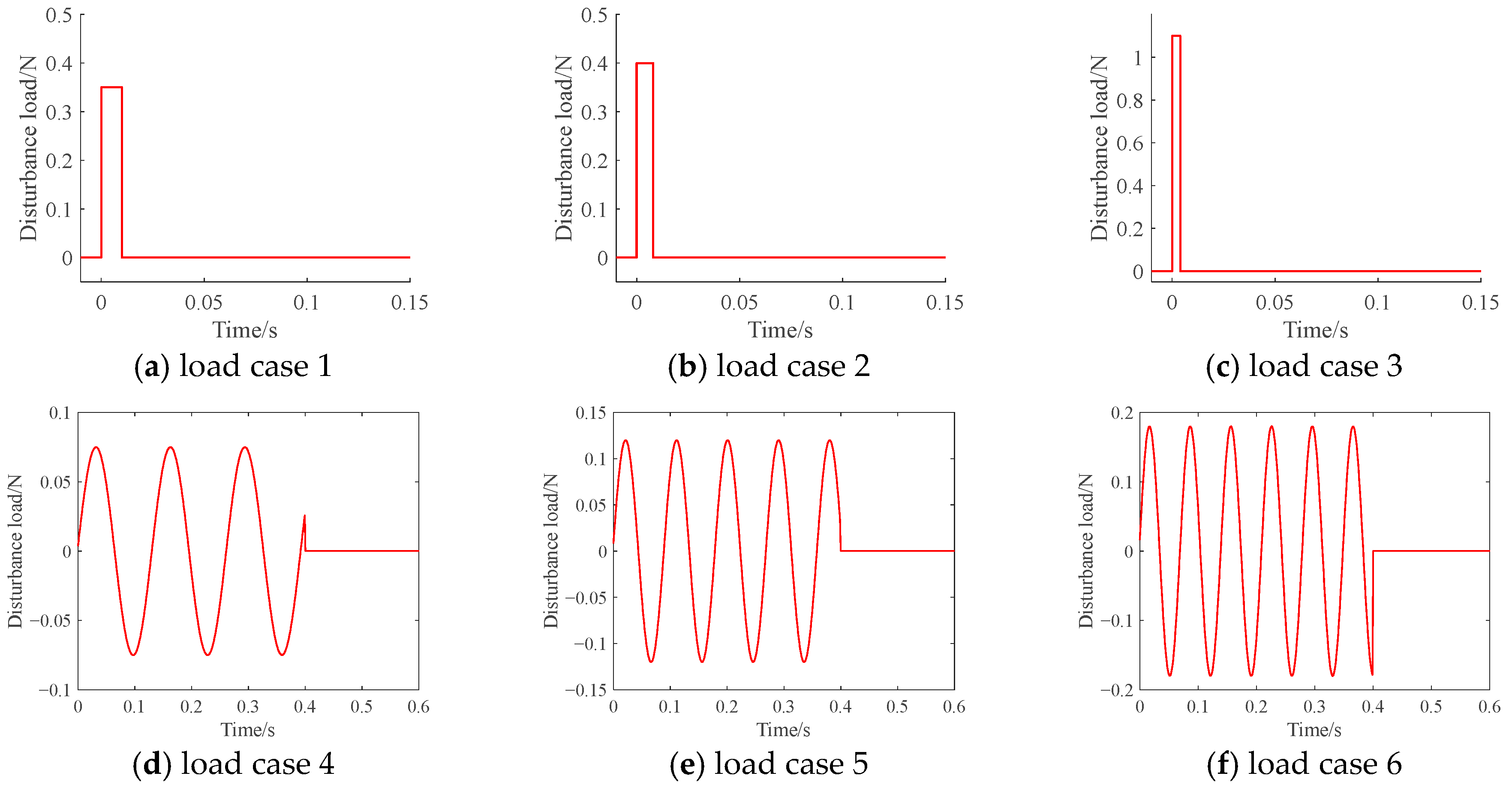
The disturbance load was applied at point A along the z-axis. The preselected load cases included 3 impact load cases, 3 sinusoidal load cases, and their corresponding loads in the opposite direction, making a total of 12 load cases with 1440 sample points. Figure 7 shows the preselected loads in the positive direction. The number of newly added samples each time was set to 4000. After adding samples 11 times, the hyper-spherical space coverage index reached $I_{hs}=0.9934$, which was greater than the required value of 0.99. The final sample set consisted of 45,440 samples, among which 40,896 samples were allocated to the training set, and both the validation set and the test set contained 2272 samples each. The radius of the control quantity interval was set as $\eta =30$. After three rounds of training, the RMSEs of the control law network were ${\sigma }_{control}=\left[\mathrm{8.2347,9.2423}\right]$, meeting the accuracy requirement of $3{\sigma }_{control}<\eta$. The total training time was 9880 s.

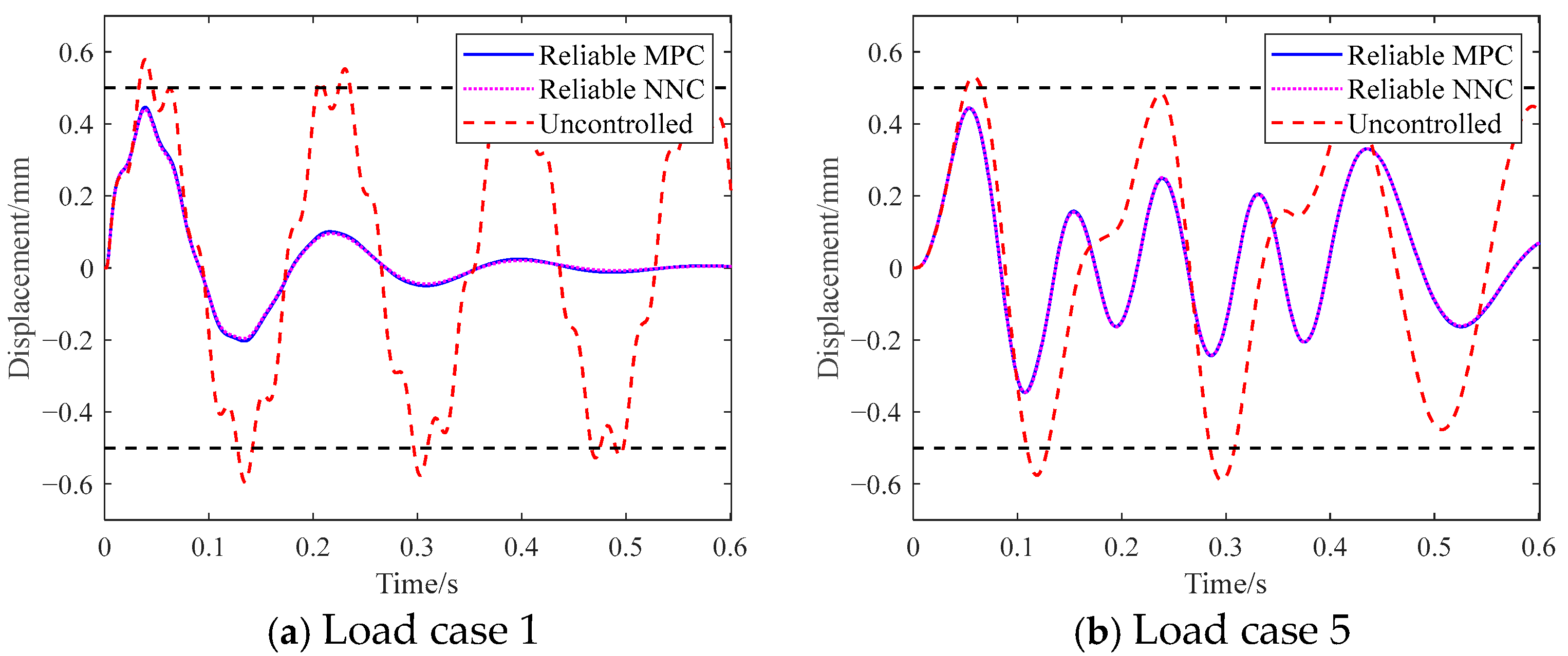
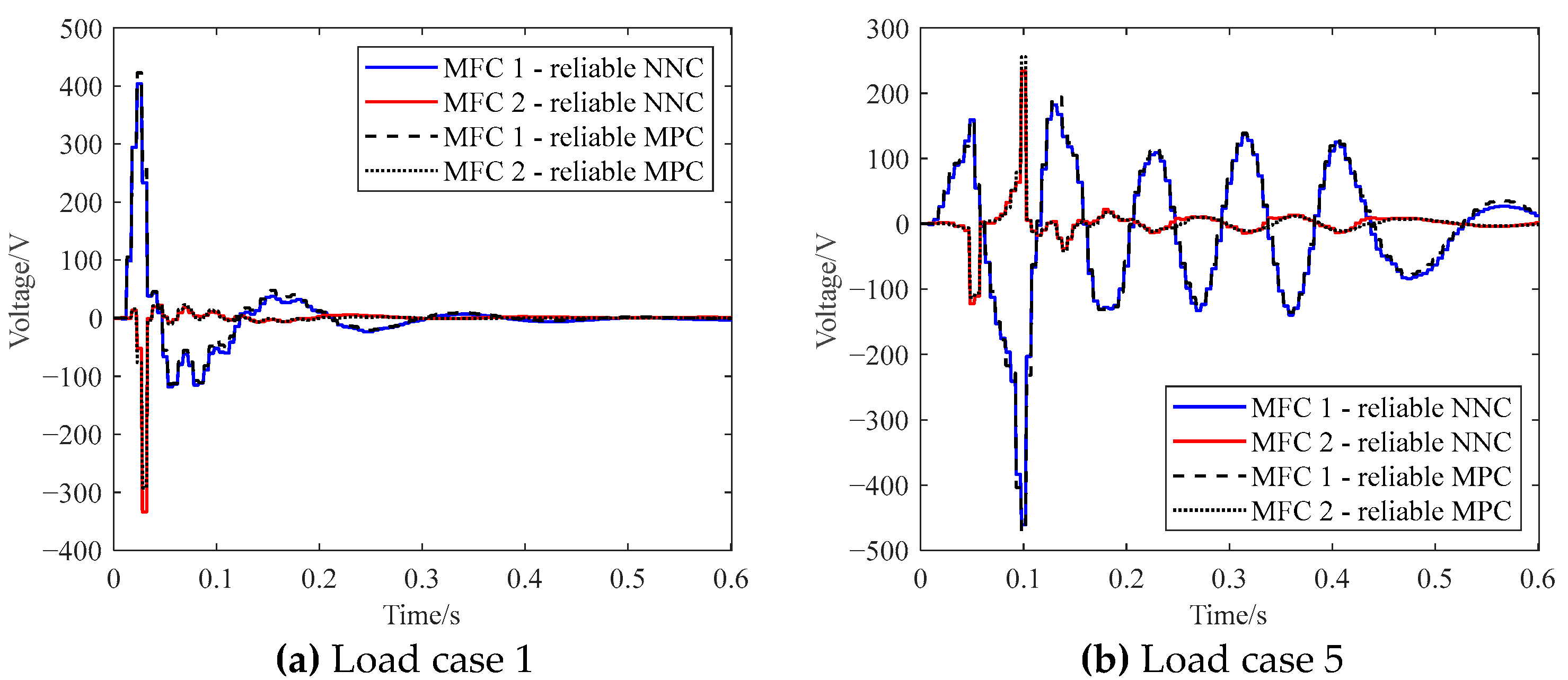
First, the control performance of the reliable NNC on preselected load conditions was verified. When the uncertain variables all took nominal values, load cases 1 and 4 were applied to the structure, and the responses obtained using the direct reliable MPC law and the reliable NNC are plotted in Figure 8. The control voltages of reliable MPC law and the reliable NNC are plotted in Figure 9. The results demonstrate that the structural responses under the two control strategies were nearly identical, confirming that the NNC law derived via deep learning can effectively approximate the reliable MPC law. The average forward calculation time of the control law neural network was 0.001883 s, which was less than the sampling period of the control law (0.006 s), meeting the real-time requirement.

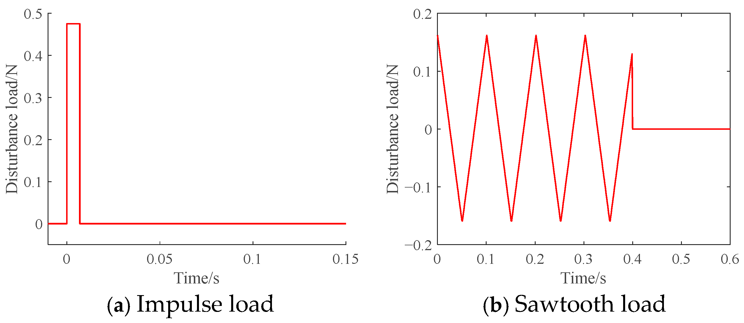
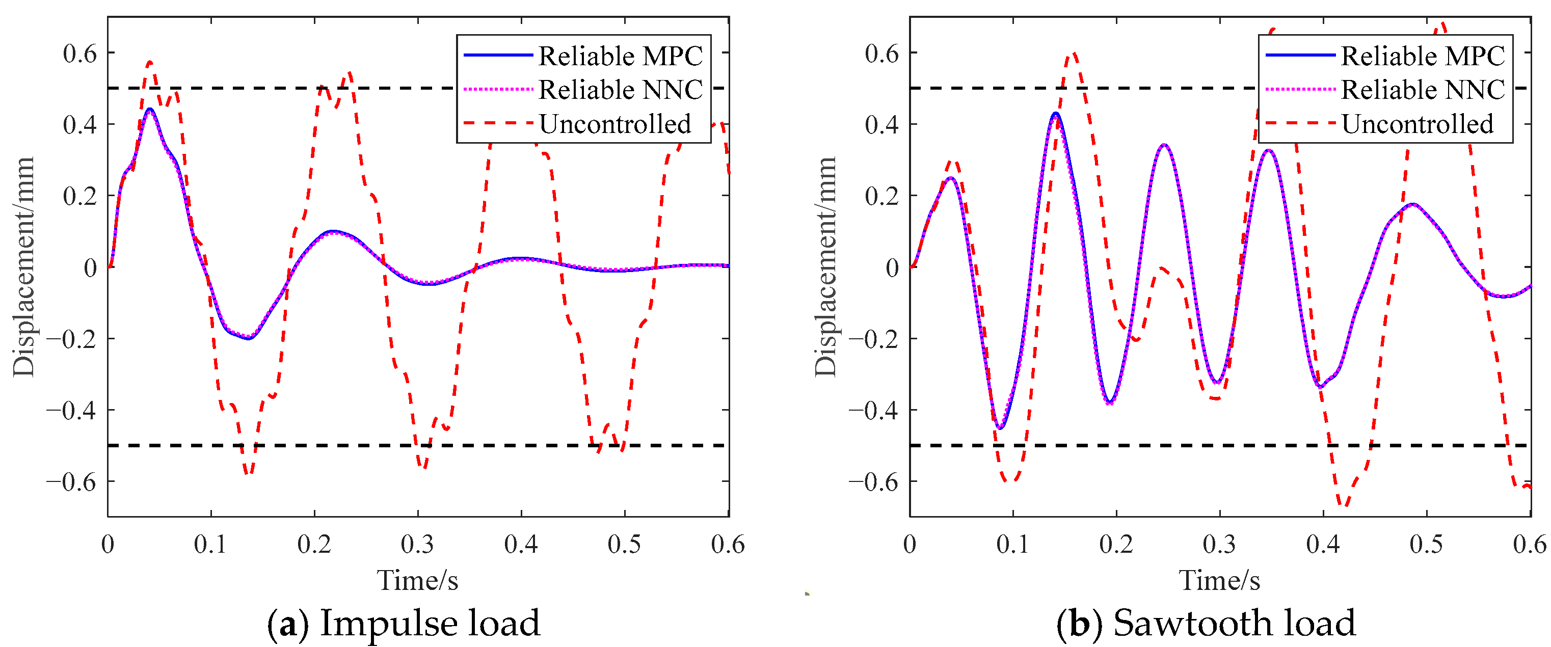
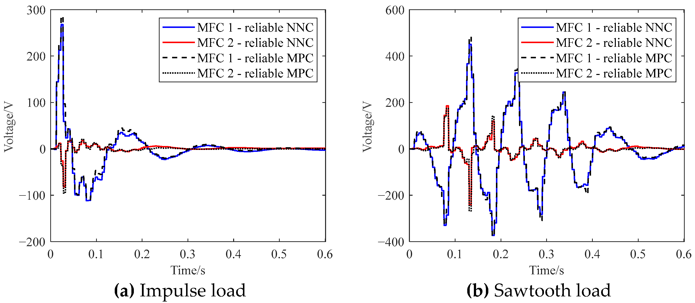
Subsequently, the control effectiveness of the reliable NCC law for non-preselected load cases was verified. Taking the impact load and sawtooth wave load shown in Figure 10 as examples, when uncertain variables take nominal values, load cases 1 and 4 were applied to the structure. The displacement responses and control voltages are plotted in Figure 11 and Figure 12, respectively. Figure 11 shows that under non-preselected loads, the learned control law still effectively suppressed vibrations. The displacement responses of the reliable MPC and the reliable NNC were basically consistent, but the deviation was slightly larger than that under preselected loads. The similar solutions observed in Figure 11 demonstrate that the reliable NNC successfully reproduced the control performance of reliable MPC as intended.

Analysis considering deviations of uncertain variables from nominal values was conducted under the sawtooth wave loading shown in Figure 10b. Figure 13 compares the displacement responses of four control laws: reliable MPC, nominal MPC, reliable neural network control, and reliability-based state feedback control [52]. When uncertain variables deviated from nominal values and take the value of $E_a=74, {\rho }_a=2850, d_{33}=430, \tau =0.008s$, the nominal MPC-controlled system exhibited displacement responses exceeding safety limits, failing to ensure safety. Concurrently, the reliability-based state feedback control law also caused significant displacement exceedance due to experiencing loads more severe than its design specifications. Although reliable MPC demonstrated slightly diminished control performance after 0.2 s, it successfully maintained Point A’s displacement within the 0.5 mm threshold during the initial 0.2 s. The reliable NNC yielded marginally larger response peaks than reliable MPC yet consistently remained below the 0.5 mm safety limit.

Finally, the nonprobabilistic reliability results of the reliable NNC, reliable MPC, nominal MPC, and reliability-based state feedback control [52] were compared. Considering impact loads with a duration of 0.08 s and amplitudes of 0.35–0.55 N (

Table 3. Comparison of nonprobabilistic reliability of different control methods under different loads.

Amplitude of Impulse Load/N	Nonprobabilistic Reliability
	Reliable NNC	Reliable MPC	Nominal MPC	Reliability-Based State Feedback Control [52]
0.35	1	1	1	1
0.375	1	1	1	1
0.4	1	1	0.9368	0.9804
0.425	1	0.9942	0.5427	0.5410
0.45	1	0.9874	0.4667	0.1710
0.475	0.9934	0.9825	0.5337	0
0.5	0.9862	0.9802	0.5851	0
0.525	0.7567	0.5896	0.4996	0
0.55	0.4658	0.3873	0.3383	0

, first column), their nonprobabilistic reliabilities under different loads are listed in Table 3 and shown in Figure 14. The nonprobabilistic reliability results in Table 3 can alternatively be interpreted as probabilistic reliability under the condition that the uncertain parameters follow uniform distributions. For the reliability-based state feedback control, reliability remained high at load amplitudes below its 0.4 N design threshold but dropped to 0 above 0.4 N. The nominal MPC shows reliability fluctuating around 0.5 for amplitudes of 0.4–0.5 N, indicating marginal constraint satisfaction. Reliable MPC maintained reliability larger than 0.98 below 0.5 N but declined above this due to exceeding actuator limits. The reliable NNC mirrored reliable MPC’s reliability trends but with slightly higher values from its conservative approximations. Compared to reliability-based state feedback control, reliable MPC ensured safety across broader loads, while the reliable NNC achieved similar adaptability with drastically reduced online computation time. The results indicate that the proposed reliable NNC can maintain structural safety under more diverse loads, highlighting its superior load adaptability compared to reliability-based state feedback control. A comparison of the four methods is listed in

Table 4. Comparison of different methods.

Method	Online Computation	Offline Computation	Reliability
Reliable NNC	Forward propagation of neural network, fast	None	More conservative than reliable MPC
Reliable MPC	Reliability-based optimization, slow	Sample generation and neural network training	Reliability assurance within actuator operational limits
Nominal MPC	Deterministic optimization, fast	None	Low reliability
Reliability-based state feedback control [52]	Multiply operation, fast	Reliability-based optimization	High-reliability only for design load Case

.

5.2. Numerical Example 2: Simplified Vertical Tail Structure

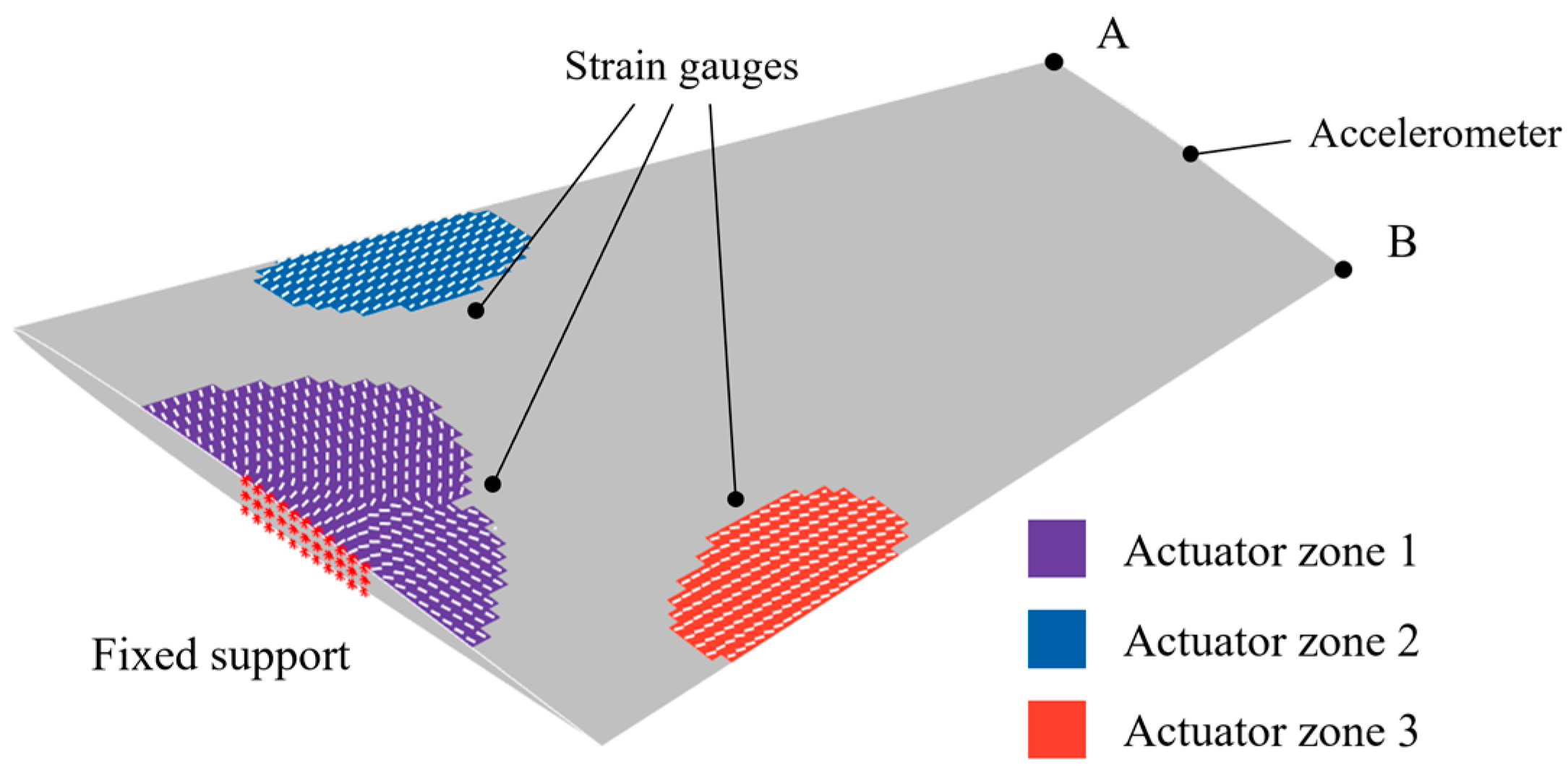
This section addresses the active vibration control of a simplified vertical tail. The vertical tail surface was covered with special-shaped piezoelectric materials, which were divided into three zones, as shown in Figure 15. A fixed boundary condition was applied to the vertical tail root, with the fixed nodes denoted by red asterisks. In this case study, the Young’s modulus $E_a$ and density ${\rho }_a$ of aluminum alloy, the piezoelectric coefficient $d_{33}$ of the piezoelectric material, and the total system time delay $\tau$ were treated as nonprobabilistic uncertain variables. Their uncertain domains are expressed as:

$${\left[\begin{array}{c}{E}_a-70\\ {\rho }_a-2700\\ d_{33}-460\\ \tau -6\\ t_{skin}-3\end{array}\right]}^{\mathrm{T}}{\left[\begin{array}{ccccc}25& 700& 0& 0& 0\\ 700& 40000& 0& 0& 0\\ 0& 0& 2500& 0& 0\\ 0& 0& 0& 4& 0\\ 0& 0& 0& 0& 0.01\end{array}\right]}^{-1}\left[\begin{array}{c}{E}_a-70\\ {\rho }_a-2700\\ d_{33}-460\\ \tau -6\\ t_{skin}-3\end{array}\right]\le 1$$

(55)

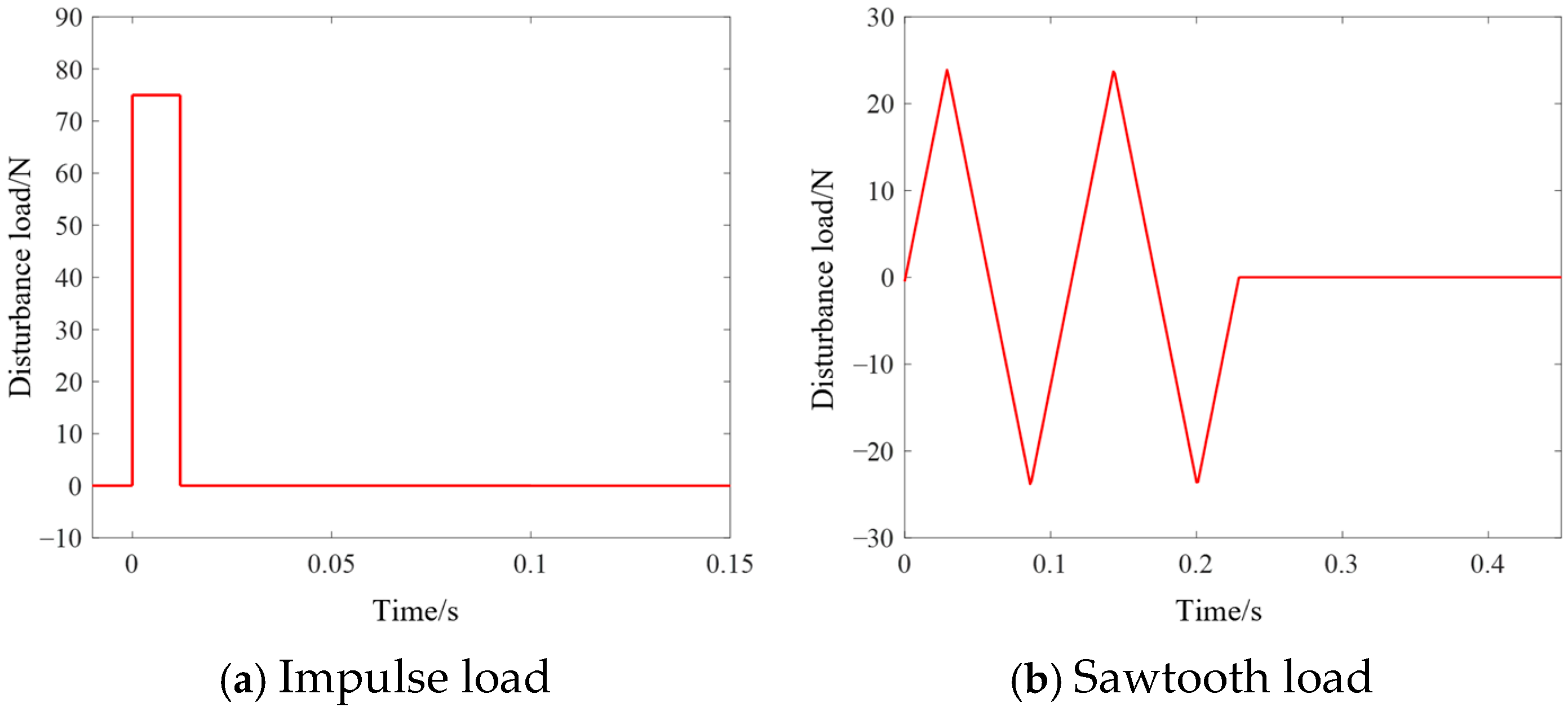
The external disturbance considered in this section is the concentrated force applied at point A along the z-direction, and the two load cases are shown in Figure 13. The limit state functions were defined as $g=1-\left|z_A\right|$ and $g=1-\left|z_B\right|$, which required that the displacements of points A and B in the z-direction should not exceed 1 mm. The nonprobabilistic reliability requirement was set to 0.98. The control voltage was constrained by $u_i\in \left[-1000,1000\right], i=1,2,3$. The sampling period of the ANKF was 0.001 s, while the sampling periods for reliable MPC was 0.003 s.

The preselected load cases include 5 impact loads, 5 sinusoidal loads, and their corresponding reverse-direction loads, totaling 20 cases with 3000 sample points. The hyper-spherical space coverage of the initial sample set is 0.0837. With 10,000 new samples added each time, after 9 rounds of sample augmentation, $I_{hs}$ was 0.9912, reaching the required threshold of 0.99. The final sample set consisted of 93,000 samples, among which 83,700 samples were allocated to the training set, and both the validation set and the test set contained 4650 samples each. The control input interval radius $\eta$ was set as 30. After 3 training iterations, the RMSE of the control law network was ${\sigma }_{control}=\left[\mathrm{8.2347,9.2423}\right]$, satisfying the accuracy requirement of $3{\sigma }_{control}<\eta$. The total training time was 97,024 s.

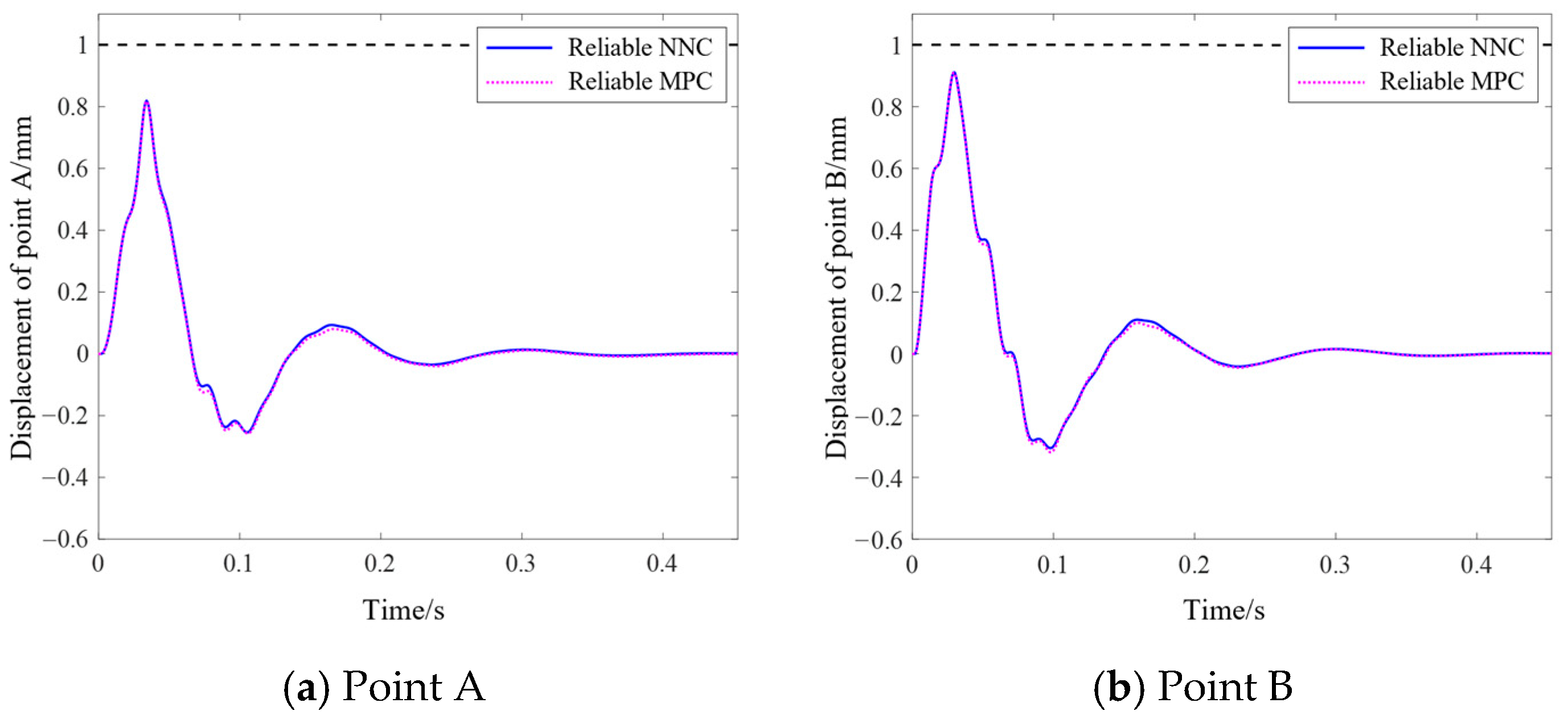
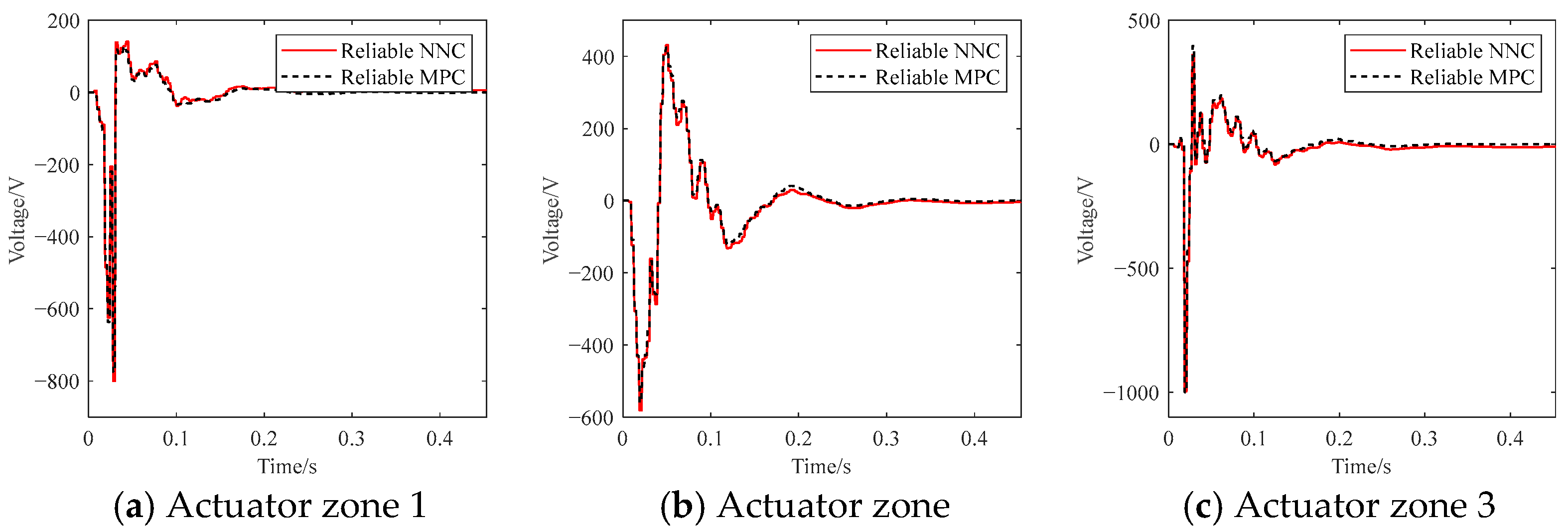
First, the control effectiveness of the proposed method for preselected load cases was verified. With all uncertain variables take their nominal values, the external disturbance load shown in Figure 16a was applied to the structure. The displacement responses obtained using the reliable MPC law and the reliable NNC are as depicted in Figure 17. The control voltages of reliable MPC law and the reliable NNC are plotted in Figure 18. The results show structural responses under the two control laws, indicating that the NNC law derived from deep learning can well fit the control law described by the samples. The average calculation time of the control law neural network was 0.002530 s, which was less than the control law’s sampling interval of 0.003 s, meeting real-time requirements.

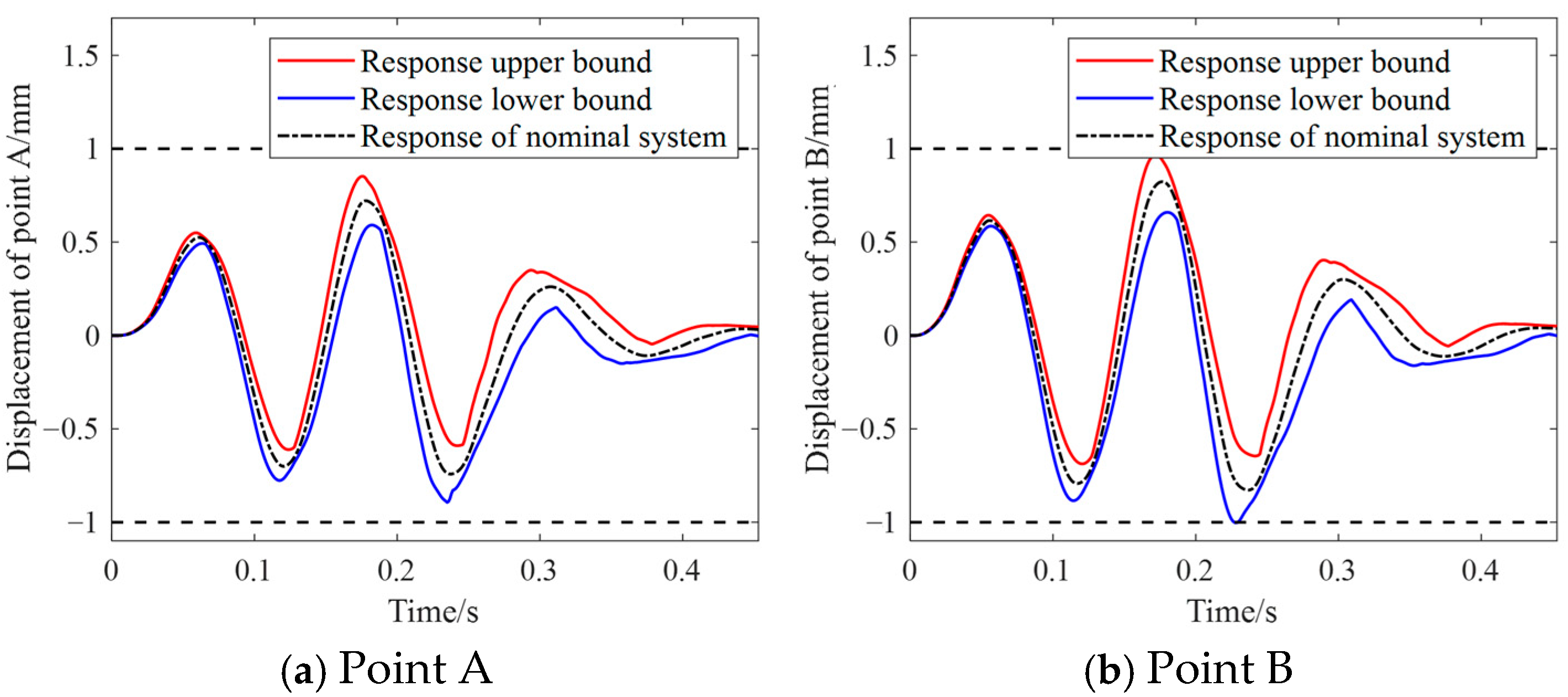
Then, the effectiveness and reliability of the reliable NNC under non-preselected loads were verified. A sawtooth load, as shown in Figure 16b and not included in the preselected cases for generating training samples, was applied to the structure. Considering uncertain parameters, Figure 19 presents the response interval bounds of the structure controlled by reliable NNC, with a nonprobabilistic reliability of 0.9934. The results demonstrate that reliable NNC effectively suppressed vibrations induced by non-preselected excitations, achieving a reliability higher than the required threshold of 0.98 for displacements remaining within the limit. This example validates that the proposed reliable NNC is applicable to active vibration control of complex structures and shows potential for practical engineering applications. When applied to systems with higher degrees of freedom, more samples, more network layers, and more neurons per layer are required to effectively describe the mapping relationships in high-dimensional spaces, which will lead to longer training time and online calculation time. To achieve approximation with similar accuracy, the required sample size typically scales exponentially with dimensionality, i.e., $t~O\left(\exp \left(2n_m+1\right)\right)$. While the proposed importance-sampling measurement reduces the growth rate below exponential, it still significantly exceeds linear scaling. Consequently, our method remains constrained by the curse of dimensionality, necessitating a trade-off between accuracy and computational tractability for high-dimensional problems.

5.3. Experimental Validation

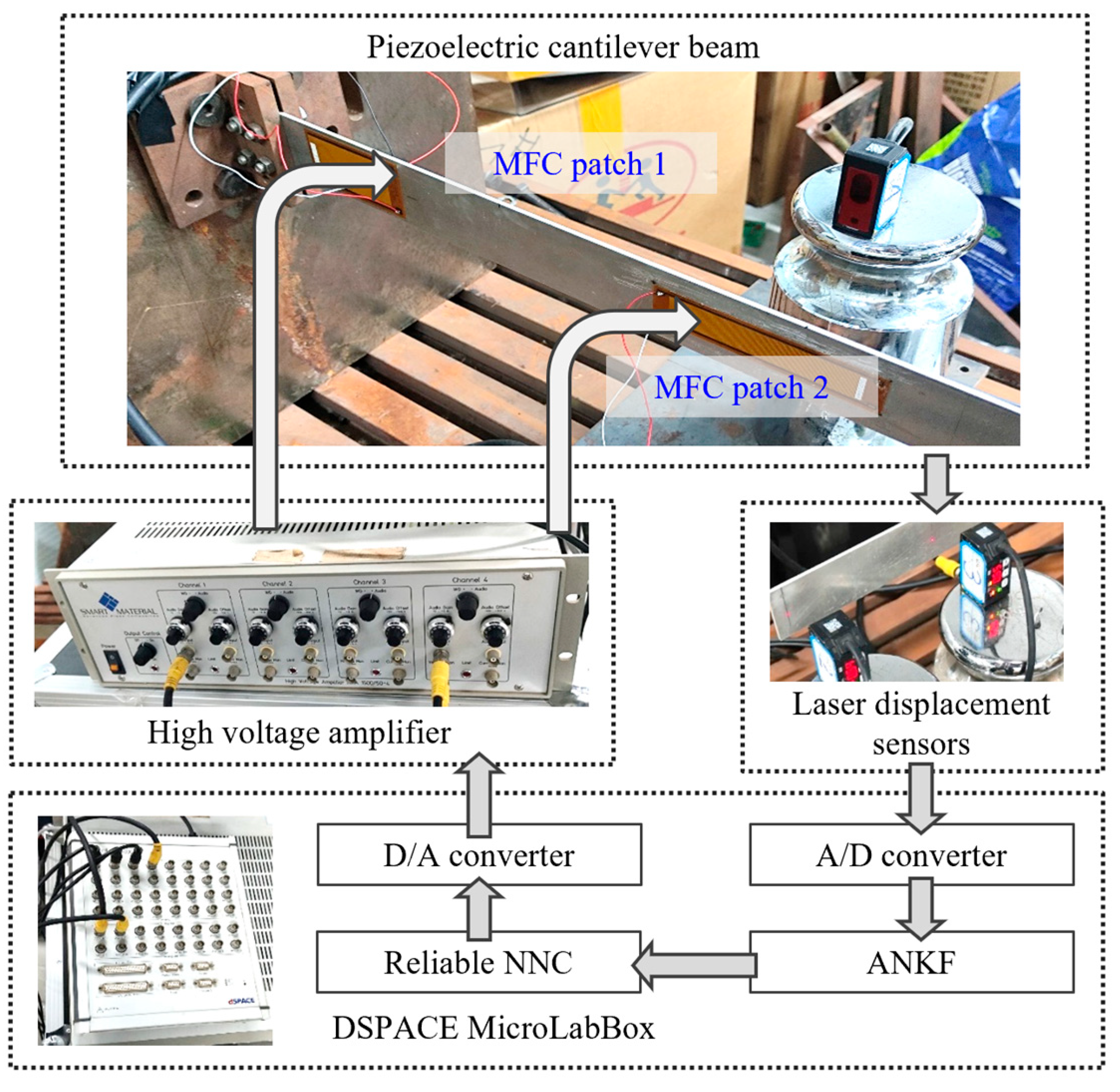
The experimental object was an aluminum alloy cantilever beam structure with MFC patches bonded to its surface. The cantilever beam had a length of 580 mm, a width of 40 mm, and a thickness of 2.6 mm (nominal value). Two piezoelectric patches were attached to the beam’s surface for vibration control: one of type M5628-P1 near the root and another of type M8514-P1 at the mid-span. Additionally, an identical M5628-P1 piezoelectric patch was bonded to the opposite side of the root patch to generate external disturbances. The reliable NNC law and nonprobabilistic Kalman filter were modeled using MATLAB and Simulink R2022b, then deployed to the control board via a dSPACE real-time interface (RTI). Control signals were amplified by a high-voltage amplifier before being applied to the MFC patches. The schematic diagram of the experimental system is shown in Figure 20.

Total time delay $\tau$, piezoelectric coefficient $k_{\mathrm{piezo}}$, and beam thickness $d_t$ were considered as uncertain parameters. Time delay was adjusted via an added loop module, and the piezoelectric coefficient change was simulated by scaling the control voltage. The time delays $\tau \in \left[0.004,0.008\right]$, scale parameter $k_{\mathrm{piezo}}\in \left[0.9,1.1\right]$, and beam thickness $d_t\in \left[2.5,2.7\right]$ were interval variables, with the limit state set as the displacement at point A not exceeding 0.5 mm: $g\left(t\right)=0.5-\left|y_A\left(t\right)\right|$. One of the piezoelectric patches was used to apply disturbances, with three load cases: (1) 360 V impulse load, (2) 500 V impulse load, and (3) sinusoidal load.

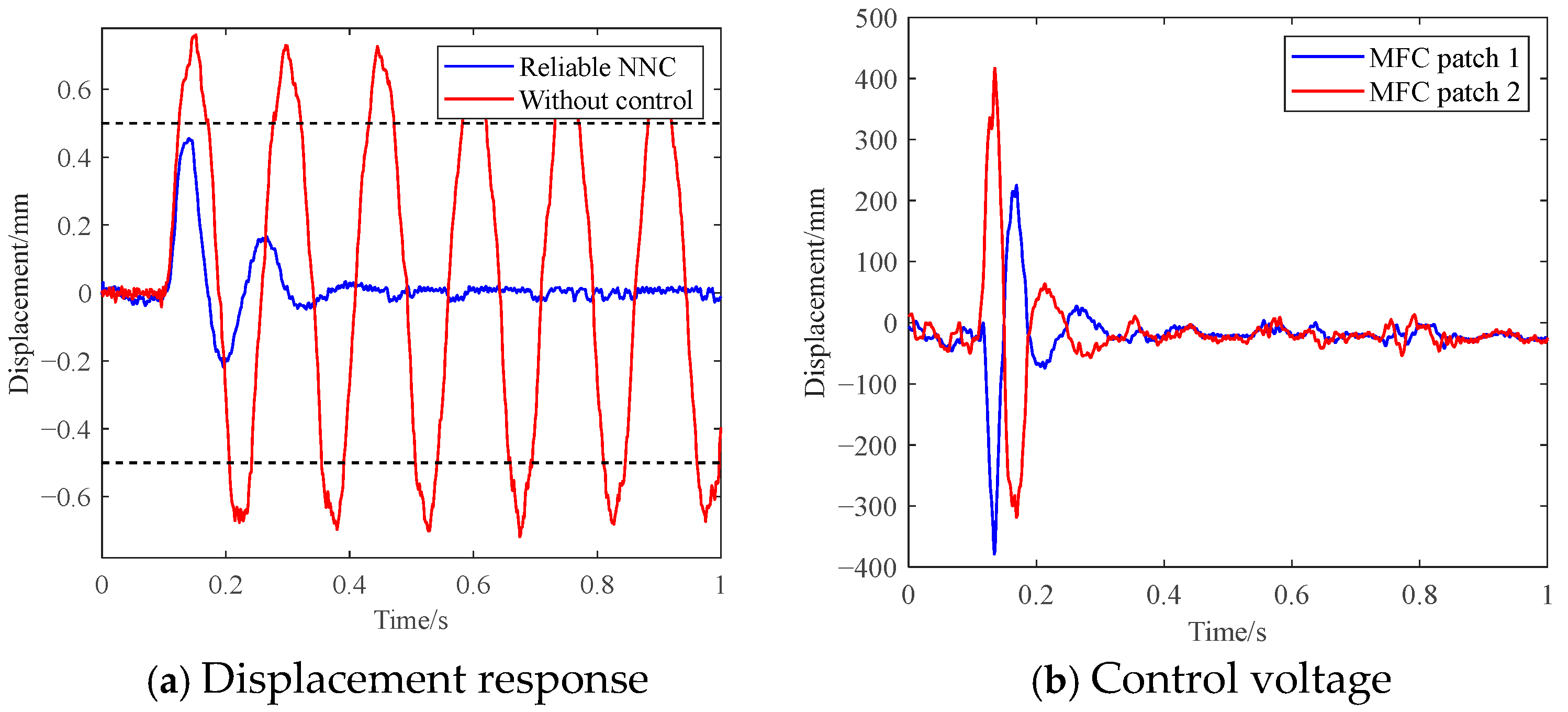
First, experiments were conducted with nominal values for uncertain variables and the load case 1. As shown in Figure 21a, without active control, the displacement response significantly exceeded the limit value, and due to the low inherent damping of the structure, the vibration decayed very slowly. After applying the reliable NNC, the displacement response remained within the limit, and the vibration was suppressed within 0.3 s, indicating that the proposed method had a good control performance on the nominal system.

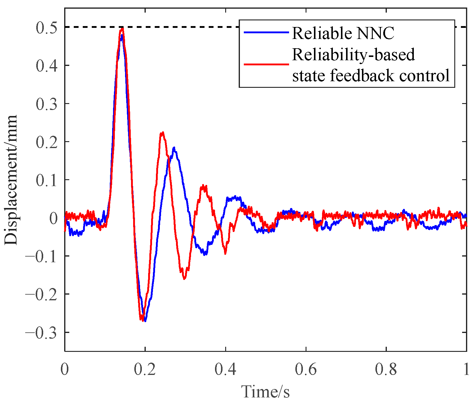
Then, the control performance of the proposed method on vibrations caused by different loads was verified. The reliability-based state feedback control was used for comparison with the proposed method, and it was designed according to the 360 V impulse load. Figure 22a,b show the displacement responses of the cantilever beam under a 500 V impulse load and a sinusoidal load, respectively. It can be seen that the reliable NNC can maintain structural safety under larger-amplitude impulse or sinusoidal loads. However, due to the applied loads being more severe than the design load, the structure with reliability-based state feedback control exhibited displacement exceeding the limit, as shown by the red lines in Figure 22. When the uncertain variables deviated from their nominal values and took the value of $\tau =0.008s,k_{\mathrm{piezo}}=0.9,d_t=2.5$, the displacement response of the cantilever beam under a 360 V impulse load is shown in Figure 23. As can be seen from Figure 23, although the control performance of the reliable NNC decreased, it still ensured that the displacement did not exceed the limit of 0.5 mm, and the reliability-based state feedback control also guaranteed the safety of the structure. The experimental results verify that the proposed reliable NNC can maintain structural safety under the influence of uncertain factors and can adapt to unknown external loads compared with the existing reliability-based state feedback control.

6. Conclusions

This study presents a reliable NNC method rooted in reliable MPC. A DNN was constructed and trained with minimum mean square error to emulate the reliable MPC law. Starting from the characteristics of the reliable MPC law, an auxiliary neural network as developed to identify whether reliability constraints for sample points were activated, accompanied by a proposed importance sampling strategy. The hyper-sphere space coverage index as employed to evaluate the effectiveness of sample points in covering the entire sample space, ensuring the NNC law’s validity under all feasible conditions.

Two numerical case studies demonstrated that the proposed method maintained the performance and external load adaptability of reliable MPC while drastically reducing online computational overhead. A piezoelectric cantilever beam vibration control experimental system was established, and vibration control experiments further validated the method’s effectiveness and advantages.

The proposed reliable NNC can ensure structural safety under a wider variety of disturbance loads, whereas existing reliability-based control methods can only achieve the required reliability under design-specified loading conditions. Future research will focus on integrating MPC with reinforcement learning for vibration control, aiming to enable active online learning and effective suppression of vibrations induced by random loads.

References

1. Preumont, A. Vibration Control of Active Structures; Solid Mechanics and Its Applications; Springer International Publishing: Cham, Switzerland, 2018; Volume 246, ISBN 978-3-319-72295-5. [Google Scholar]
2. Gardonio, P. Review of Active Techniques for Aerospace Vibro-Acoustic Control. J. Aircr. 2002, 39, 206–214. [Google Scholar] [CrossRef]
3. He, W.; Ouyang, Y.; Hong, J. Vibration Control of a Flexible Robotic Manipulator in the Presence of Input Deadzone. IEEE Trans. Ind. Inform. 2017, 13, 48–59. [Google Scholar] [CrossRef]
4. Zhang, H.; Wang, R.; Wang, J.; Shi, Y. Robust Finite Frequency Static-Output-Feedback Control with Application to Vibration Active Control of Structural Systems. Mechatronics 2014, 24, 354–366. [Google Scholar] [CrossRef]
5. Karkoub, M.; Balas, G.; Tamma, K.; Donath, M. Robust Control of Fexible Manipulators via μ-Synthesis. Control Eng. Pract. 2000, 8, 725–734. [Google Scholar] [CrossRef]
6. Chen, Z.; Yao, B.; Wang, Q. μ-Synthesis-Based Adaptive Robust Control of Linear Motor Driven Stages with High-Frequency Dynamics: A Case Study. IEEE ASME Trans. Mechatron. 2015, 20, 1482–1490. [Google Scholar] [CrossRef]
7. Brand, Z.; Cole, M.O.T. Mini-Max Optimization of Actuator/Sensor Placement for Flexural Vibration Control of a Rotating Thin-Walled Cylinder over a Range of Speeds. J. Sound Vib. 2021, 506, 116105. [Google Scholar] [CrossRef]
8. Choi, D. Min-Max Control for Vibration Suppression of Mobile Manipulator with Active Suspension System. Int. J. Control Autom. Syst. 2022, 20, 618–626. [Google Scholar] [CrossRef]
9. Rodriguez, J.; Collet, M.; Chesné, S. Active Vibration Control on a Smart Composite Structure Using Modal-Shaped Sliding Mode Control. J. Vib. Acoust. 2022, 144, 21013. [Google Scholar] [CrossRef]
10. Qing-lei Hu; Zidong Wang; Huijun Gao Sliding Mode and Shaped Input Vibration Control of Flexible Systems. IEEE Trans. Aerosp. Electron. Syst. 2008, 44, 503–519. [CrossRef]
11. Lu, Q.; Wang, P.; Liu, C. An Analytical and Experimental Study on Adaptive Active Vibration Control of Sandwich Beam. Int. J. Mech. Sci. 2022, 232, 107634. [Google Scholar] [CrossRef]
12. Landau, I.D.; Airimițoaie, T.-B.; Castellanos-Silva, A.; Constantinescu, A. Adaptive and Robust Active Vibration Control: Methodology and Tests; Advances in Industrial Control; Springer International Publishing: Cham, Switzerland, 2017; ISBN 978-3-319-41449-2. [Google Scholar]
13. Liu, Z.; Liu, J.; He, W. An Adaptive Iterative Learning Algorithm for Boundary Control of a Flexible Manipulator. Int. J. Adapt. Control Signal Process. 2017, 31, 903–916. [Google Scholar] [CrossRef]
14. Wang, C.; Zheng, M.; Wang, Z.; Peng, C.; Tomizuka, M. Robust Iterative Learning Control for Vibration Suppression of Industrial Robot Manipulators. J. Dyn. Syst. Meas. Control 2018, 140, 11003. [Google Scholar] [CrossRef]
15. Pisarski, D.; Jankowski, Ł. Reinforcement Learning-based Control to Suppress the Transient Vibration of Semi-active Structures Subjected to Unknown Harmonic Excitation. Comput.-Aided Civ. Infrastruct. Eng. 2023, 38, 1605–1621. [Google Scholar] [CrossRef]
16. Qiu, Z.; Yang, Y.; Zhang, X. Reinforcement Learning Vibration Control of a Multi-Flexible Beam Coupling System. Aerosp. Sci. Technol. 2022, 129, 107801. [Google Scholar] [CrossRef]
17. Crespo, L.G.; Kenny, S.P. Reliability-Based Control Design for Uncertain Systems. J. Guid. Control Dyn. 2005, 28, 649–658. [Google Scholar] [CrossRef]
18. Li, Y.; Xu, M.; Chen, J.; Wang, X. Nonprobabilistic Reliable LQR Design Method for Active Vibration Control of Structures with Uncertainties. AIAA J. 2018, 56, 2443–2454. [Google Scholar] [CrossRef]
19. Yang, C.; Lu, W.; Xia, Y. Positioning Accuracy Analysis of Industrial Robots Based on Non-Probabilistic Time-Dependent Reliability. IEEE Trans. Reliab. 2024, 73, 608–621. [Google Scholar] [CrossRef]
20. Gorla, A.; Serkies, P. Comparative Study of Analytical Model Predictive Control and State Feedback Control for Active Vibration Suppression of Two-Mass Drive. Actuators 2025, 14, 254. [Google Scholar] [CrossRef]
21. Li, H.; Shi, Y. Distributed Receding Horizon Control of Large-Scale Nonlinear Systems: Handling Communication Delays and Disturbances. Automatica 2014, 50, 1264–1271. [Google Scholar] [CrossRef]
22. Li, H.; Shi, Y. Robust Distributed Model Predictive Control of Constrained Continuous-Time Nonlinear Systems: A Robustness Constraint Approach. IEEE Trans. Autom. Control 2014, 59, 1673–1678. [Google Scholar] [CrossRef]
23. Scokaert, P.O.M.; Mayne, D.Q. Min-Max Feedback Model Predictive Control for Constrained Linear Systems. IEEE Trans. Autom. Control 1998, 43, 1136–1142. [Google Scholar] [CrossRef]
24. Kerrigan, E.C.; Maciejowski, J.M. Feedback Min-max Model Predictive Control Using a Single Linear Program: Robust Stability and the Explicit Solution. Int. J. Robust Nonlinear Control 2004, 14, 395–413. [Google Scholar] [CrossRef]
25. Raković, S.V.; Kouvaritakis, B.; Cannon, M.; Panos, C. Fully Parameterized Tube Model Predictive Control: FULLY PARAMETERIZED TUBE MPC. Int. J. Robust Nonlinear Control 2012, 22, 1330–1361. [Google Scholar] [CrossRef]
26. Kohler, J.; Soloperto, R.; Muller, M.A.; Allgower, F. A Computationally Efficient Robust Model Predictive Control Framework for Uncertain Nonlinear Systems. IEEE Trans. Autom. Control 2021, 66, 794–801. [Google Scholar] [CrossRef]
27. Mayne, D.Q.; Kerrigan, E.C.; Falugi, P. Robust Model Predictive Control: Advantages and Disadvantages of Tube-Based Methods. IFAC Proc. Vol. 2011, 44, 191–196. [Google Scholar] [CrossRef]
28. Hajiloo, A.; Xie, W.F. The Stochastic Robust Model Predictive Control of Shimmy Vibration in Aircraft Landing Gears: The Stochastic Robust Model Predictive Control. Asian J. Control 2015, 17, 476–485. [Google Scholar] [CrossRef]
29. Schildbach, G.; Calafiore, G.C.; Fagiano, L.; Morari, M. Randomized Model Predictive Control for Stochastic Linear Systems. In Proceedings of the 2012 American Control Conference (ACC), Montreal, QC, Canada, 27–29 June 2012; IEEE: New York, NY, USA, 2012; pp. 417–422. [Google Scholar]
30. Mesbah, A. Stochastic Model Predictive Control: An Overview and Perspectives for Future Research. IEEE Control Syst. 2016, 36, 30–44. [Google Scholar] [CrossRef]
31. Dai, L.; Yu, Y.; Zhai, D.-H.; Huang, T.; Xia, Y. Robust Model Predictive Tracking Control for Robot Manipulators with Disturbances. IEEE Trans. Ind. Electron. 2021, 68, 4288–4297. [Google Scholar] [CrossRef]
32. Chen, Y.; Zhang, S.; Peng, H.; Chen, B.; Zhang, H. A Novel Fast Model Predictive Control for Large-Scale Structures. J. Vib. Control 2017, 23, 2190–2205. [Google Scholar] [CrossRef]
33. Wang, E.; Wu, S.; Xun, G.; Liu, Y.; Wu, Z. Active Vibration Suppression for Large Space Structure Assembly: A Distributed Adaptive Model Predictive Control Approach. J. Vib. Control 2021, 27, 365–377. [Google Scholar] [CrossRef]
34. Dubay, R.; Hassan, M.; Li, C.; Charest, M. Finite Element Based Model Predictive Control for Active Vibration Suppression of a One-Link Flexible Manipulator. ISA Trans. 2014, 53, 1609–1619. [Google Scholar] [CrossRef] [PubMed]
35. Alessio, A.; Bemporad, A. A Survey on Explicit Model Predictive Control. In Nonlinear Model Predictive Control: Towards New Challenging Applications; Magni, L., Raimondo, D.M., Allgöwer, F., Eds.; Springer: Berlin/Heidelberg, Germany, 2009; pp. 345–369. ISBN 978-3-642-01094-1. [Google Scholar]
36. Takács, G.; Rohal’-Ilkiv, B. MPC Implementation for Vibration Control. In Model Predictive Vibration Control; Springer: London, UK, 2012; pp. 361–389. ISBN 978-1-4471-2332-3. [Google Scholar]
37. Gulan, M.; Takács, G.; Nguyen, N.A.; Olaru, S.; Rodríguez-Ayerbe, P.; Rohal’-Ilkiv, B. Efficient Embedded Model Predictive Vibration Control via Convex Lifting. IEEE Trans. Control Syst. Technol. 2019, 27, 48–62. [Google Scholar] [CrossRef]
38. Bemporad, A.; Oliveri, A.; Poggi, T.; Storace, M. Ultra-Fast Stabilizing Model Predictive Control via Canonical Piecewise Affine Approximations. IEEE Trans. Autom. Control 2011, 56, 2883–2897. [Google Scholar] [CrossRef]
39. Parisini, T.; Zoppoli, R. A Receding-Horizon Regulator for Nonlinear Systems and a Neural Approximation. Automatica 1995, 31, 1443–1451. [Google Scholar] [CrossRef]
40. Aslam, S.; Chak, Y.-C.; Jaffery, M.H.; Varatharajoo, R.; Razoumny, Y. Deep Learning Based Fuzzy-MPC Controller for Satellite Combined Energy and Attitude Control System. Adv. Space Res. 2024, 74, 3234–3255. [Google Scholar] [CrossRef]
41. Gómez, P.I.; Gajardo, M.E.L.; Mijatovic, N.; Dragičević, T. Enhanced Imitation Learning of Model Predictive Control through Importance Weighting. IEEE Trans. Ind. Electron. 2024, 72, 4073–4083. [Google Scholar] [CrossRef]
42. Wen, C.; Ma, X.; Erik Ydstie, B. Analytical Expression of Explicit MPC Solution via Lattice Piecewise-Affine Function. Automatica 2009, 45, 910–917. [Google Scholar] [CrossRef]
43. Cseko, L.H.; Kvasnica, M.; Lantos, B. Explicit MPC-Based RBF Neural Network Controller Design with Discrete-Time Actual Kalman Filter for Semiactive Suspension. IEEE Trans. Control Syst. Technol. 2015, 23, 1736–1753. [Google Scholar] [CrossRef]
44. Hertneck, M.; Kohler, J.; Trimpe, S.; Allgower, F. Learning an Approximate Model Predictive Controller with Guarantees. IEEE Control Syst. Lett. 2018, 2, 543–548. [Google Scholar] [CrossRef]
45. Li, Y.; Hua, K.; Cao, Y. Using Stochastic Programming to Train Neural Network Approximation of Nonlinear MPC Laws. Automatica 2022, 146, 110665. [Google Scholar] [CrossRef]
46. Ben-Haim, Y. A Non-Probabilistic Concept of Reliability. Struct. Saf. 1994, 14, 227–245. [Google Scholar] [CrossRef]
47. Jiang, C.; Li, J.W.; Ni, B.Y.; Fang, T. Some Significant Improvements for Interval Process Model and Non-Random Vibration Analysis Method. Comput. Methods Appl. Mech. Eng. 2019, 357, 112565. [Google Scholar] [CrossRef]
48. Du, H.; Zhang, N.; Naghdy, F. Actuator Saturation Control of Uncertain Structures with Input Time Delay. J. Sound Vib. 2011, 330, 4399–4412. [Google Scholar] [CrossRef]
49. Gong, J.; Wang, X. Reliable Model Predictive Vibration Control for Structures with Nonprobabilistic Uncertainties. Struct. Control Health Monit. 2024, 2024, 7596923. [Google Scholar] [CrossRef]
50. Karg, B.; Lucia, S. Reinforced Approximate Robust Nonlinear Model Predictive Control. In Proceedings of the 2021 23rd International Conference on Process Control (PC), Strbske Pleso, Slovakia, 1–4 June 2021; IEEE: New York, NY, USA, 2021; pp. 149–156. [Google Scholar]
51. Liu, Z.; Ji, H.; Wu, Y.; Zhang, C.; Tao, C.; Qiu, J. Design of a High-Voltage Miniaturized Control System for Macro Fiber Composites Actuators. Actuators 2024, 13, 509. [Google Scholar] [CrossRef]
52. Yang, C. Interval Riccati Equation-Based and Non-Probabilistic Dynamic Reliability-Constrained Multi-Objective Optimal Vibration Control with Multi-Source Uncertainties. J. Sound Vib. 2025, 595, 118742. [Google Scholar] [CrossRef]
Figure 1. Overview of the proposed reliable NNC architecture.
Actuators 14 00402 g001
Figure 2. Illustration of the reliable MPC law.
Actuators 14 00402 g002
Figure 3. Schematic plot of the importance sampling strategy.
Actuators 14 00402 g003
Figure 4. The flowchart of training the reliable NNC law.
Actuators 14 00402 g004
Figure 5. Flowchart of the ANKF.
Actuators 14 00402 g005
Figure 6. Schematic plot of the cantilever beam.
Actuators 14 00402 g006
Figure 7. The disturbance load amplitude of preselected load cases.
Actuators 14 00402 g007
Figure 8. Displacement responses under preselected load cases.
Actuators 14 00402 g008
Figure 9. Control voltages under preselected load cases.
Actuators 14 00402 g009
Figure 10. The disturbance load amplitude of non-preselected load cases.
Actuators 14 00402 g010
Figure 11. Displacement response under the non-preselected load cases.
Actuators 14 00402 g011
Figure 12. Control voltages under the non-preselected load cases.
Actuators 14 00402 g012
Figure 13. Displacement responses under the condition of uncertain variables deviating from nominal values.
Actuators 14 00402 g013
Figure 14. Comparison of nonprobabilistic reliability of different control methods under different loads.
Actuators 14 00402 g014
Figure 15. Schematic diagram of the simplified vertical tail structure.
Actuators 14 00402 g015
Figure 16. Amplitude of external disturbance loads acting on the tail wing structure.
Actuators 14 00402 g016
Figure 17. Displacement responses of the tail wing under preselected impulse load.
Actuators 14 00402 g017
Figure 18. Control voltages of the tail wing under preselected impulse load.
Actuators 14 00402 g018
Figure 19. Displacement response interval bounds of the tail wing under non-preselected load.
Actuators 14 00402 g019
Figure 20. Schematic diagram of the experimental system.
Actuators 14 00402 g020
Figure 21. Experimental results of displacement response and control voltage under load case 1.
Actuators 14 00402 g021
Figure 22. Experimental results of displacement responses under different load cases.
Actuators 14 00402 g022
Figure 23. Experimental results of displacement responses under the influence of uncertain parameters.
Actuators 14 00402 g023