Article

A Novel Kinematic Calibration Method for Industrial Robots Based on the Improved Grey Wolf Optimization Algorithm

by
Bingzhang Cao
1,
Jiuwei Yu
1,
Yi Zhang
1,
Peijun Liu
1,
Yifan Zhang
1,
Hongwei Sun
1,
Peng Jin
1,
Jie Lin
2 and
Lei Wang
1,*
1
Key Laboratory of Micro-Systems and Micro-Structures Manufacturing, Ministry of Education, Harbin Institute of Technology, Harbin 150001, China
2
School of Physics, Harbin Institute of Technology, Harbin 150001, China
*
Author to whom correspondence should be addressed.
Actuators 2025, 14(8), 403; https://doi.org/10.3390/act14080403
Submission received: 1 July 2025 / Revised: 9 August 2025 / Accepted: 11 August 2025 / Published: 13 August 2025
(This article belongs to the Special Issue Intelligent Sensing, Control and Actuation in Networked Systems)

Abstract

Due to insufficient absolute positioning accuracy, industrial robots frequently face challenges in efficiently performing drilling and riveting operations during the assembly of aircraft and other large-scale workpieces. To enhance the absolute positioning accuracy of industrial robots, this paper proposes a novel kinematic calibration method for industrial robots based on the Improved Grey Wolf Optimization (IGWO) algorithm. Specifically, the method employs an enhanced selection and update strategy to avoid convergence stagnation and local optimum traps. The proposed method features a novel boundary search strategy, which leverages the Dimension-oriented Learning (DL) search strategy to enhance search speed and stability. Through parameter identification and calibration experiments, the effectiveness of the method was validated using an ABB IRB4600 industrial robot and a Leica laser tracker. Additionally, compared with the Levenberg–Marquardt (LM) algorithm, Particle Swarm Optimization (PSO), and Genetic Algorithm (GA), the IGWO algorithm demonstrates faster convergence and superior optimization performance. According to the calibration experimental results, by applying the IGWO algorithm, the absolute positioning accuracy of the industrial robot is ultimately improved from 1.918 mm to 0.475 mm and the absolute positioning accuracy is improved by 75.2%.

1. Introduction

Component assembly constitutes a critical process in aircraft manufacturing, serving as the final step to ensure the operational performance of the aircraft. This stage accounts for over 50% of the total workload and incurs costs ranging from 35% to 45% of the total manufacturing cost [1,2]. During the assembly process, a considerable number of connection holes need to be drilled and riveted to achieve component joining. The quality of drilling and riveting significantly impacts the fatigue life of connectors and the overall production efficiency [3]. To enhance drilling–riveting accuracy, reduce damage, and minimize uncertainties caused by manual operations, industrial robot-based automatic drilling–riveting technology has been widely adopted in aircraft assembly.
Industrial robot automatic drilling–riveting systems leverage the robot’s advantages of high flexibility, high integration, a small footprint, and a large work envelope. Equipped with multi-functional end-effectors, industrial robots can perform automated drilling and riveting on aircraft production lines, featuring fast processing speeds and simple operations [4]. This has substantially improved the efficiency and economic benefits of aircraft automated assembly, leading to the extensive application of industrial robots in the aircraft manufacturing industry [5]. Although industrial robots typically achieve a repeatability of up to ±0.1 mm [6], their absolute positioning accuracy is only ±2–3 mm. However, aircraft assembly technology often requires absolute positioning accuracy below 0.6 mm [7,8,9], thus necessitating the calibration of industrial robots.
Currently, offline calibration is the most widely adopted approach to improve the absolute positioning accuracy of industrial robots in practical manufacturing systems [10]. Factors affecting absolute positioning accuracy are numerous, primarily stemming from environmental factors (temperature or preheating processes), parameter errors (kinematic parameter variations due to manufacturing and assembly errors; dynamic parameter influences), measurement uncertainties (resolution and nonlinear errors of joint position sensors), computational errors (computer correction and steady-state control errors), and application-related factors (installation errors) [11]. Among these, kinematic parameter errors play a dominant role in the total positioning errors of industrial robots [12]. Therefore, calibrating the kinematic parameters of industrial robots can effectively enhance their absolute positioning accuracy.
Over the past few decades, extensive research has been conducted on the kinematic parameter calibration of robots [13,14]. Jiang et al. [15] employed the extended Kalman filter and particle filter algorithms to identify the kinematic parameters of a Kawasaki RS10N robot, achieving an improvement in absolute positioning accuracy with the positioning error reduced from 3.1407 mm to 0.263 mm after calibration. Gao et al. [16] proposed a novel hybrid algorithm combining BP neural networks and Particle Swarm Optimization (PSO) for kinematic parameter identification, improving the positioning accuracy of the ER20-C10 robot to 0.4 mm after parameter error compensation. Luo et al. [17] developed a calibration method based on a hybrid algorithm of Levenberg–Marquardt (LM) and Differential Evolution (DE) to calculate kinematic parameter deviations, and comprehensive experiments on a FANUC M710ic/50 industrial robot showed that the method significantly enhanced the calibration accuracy of the robot arm.
Meanwhile, meta-heuristic optimization algorithms have been applied to kinematic calibration of industrial robots, as they can search for approximate optimal solutions through iterative searching and diversity strategies. Zhong et al. [18] used an Improved Whale Optimization (IWO) algorithm to calibrate a two-segment hydraulic mechanical leg, successfully obtaining kinematic parameter deviations. The results showed that the algorithm featured fast search speed and avoided local optimization traps, though it involved complex calculations. Li et al. [19] combined the extended Kalman filter with a quadratic interpolation beetle antenna search algorithm to calibrate robots, searching for optimal kinematic parameters and improving the absolute positioning accuracy of an ABB IRB120 industrial robot by 5.17%. Chen et al. [20] proposed a kinematic calibration method based on an Improved Beetle Swarm Optimization (IBSO) algorithm, verifying its effectiveness through simulation and calibration experiments on a KUKA KR500L340-2 industrial robot system.
While these methods can calibrate robot parameters and improve positioning accuracy to varying degrees, each has its own advantages and disadvantages in terms of the comprehensive consideration of calibration accuracy and efficiency. Therefore, developing new calibration methods can provide more options for industrial robots in different fields to enhance their positioning accuracy, which holds significant practical application value.
The robot kinematic model is a highly nonlinear system, typically linearized by neglecting second-order and higher-order error terms, followed by rapid identification of kinematic parameters using the least squares method [21]. However, this introduces linear truncation errors, causing the LM algorithm to perform poorly on highly nonlinear systems, especially leading to stagnation when approaching the optimal solution. The Grey Wolf Optimization (GWO) algorithm, a population-based global search optimizer, effectively addresses nonlinear problems due to its high reliability, strong robustness, and superior optimization performance. Nevertheless, the need to identify numerous kinematic parameters and the computational complexity lead to issues such as poor stability, slow convergence, and vulnerability to local optima in the GWO algorithm [22].
To address the above issues and further improve the absolute positioning accuracy of industrial robots, this paper proposes a novel kinematic calibration method for industrial robots based on the Improved Grey Wolf Optimization (IGWO) algorithm, built upon the established robot kinematic error model. By introducing a Dimension-oriented Learning (DL) search strategy into the traditional GWO algorithm, the stability and the optimization performance of the algorithm are significantly enhanced. Experimental validation, conducted using an ABB IRB4600 robot, confirms the effectiveness and correctness of the proposed method.
The remaining sections of this paper are structured as follows. Section 2 establishes the calibration model and fitness objective function for industrial robots. Section 3 elaborates on the kinematic calibration method for industrial robots employing IGWO in detail. Section 4 validates the effectiveness of the proposed method through error compensation experiments and compares it with three other optimization algorithms. The conclusions of this paper are presented in Section 5.

2. Kinematic Error Parameter Calibration Model

This section first establishes the kinematic model and error model of typical industrial robots, then transforms the calibration problem into an optimization problem. Additionally, the objective fitness function to be solved in the optimization problem is provided.

2.1. Kinematic Model of Industrial Robot

In general, the calibration process of industrial robots involves four fundamental steps: error modeling, measurement, parameter identification, and error compensation. This paper employs the most commonly used robot kinematic modeling approach, namely the Denavit–Hartenberg (DH) method proposed by Denavit and Hartenberg, to establish the kinematic model of industrial robots. This method uses four link parameters to describe the kinematic relationships between robot arm joints, where α, a, d, and θ denote the link twist angle, link length, link offset, and joint angle, respectively [23,24,25,26,27]. Equation (1) shows the calculation method of the transformation matrix T i 1 i from link i to link i − 1, and the transformation matrix Ai is expressed as Equation (2).
T i 1 i = A i = R o t ( X , α i 1 ) T r a n s ( X , a i 1 ) T r a n s ( Z , d i ) R o t ( Z , θ i )
A i = cos θ i sin θ i cos α i sin θ i sin α i a i cos θ i sin θ i cos θ i cos α i cos θ i sin α i a i sin θ i 0 sin α i cos α i d i 0 0 0 1
By consecutively multiplying the transformation matrices, the transformation matrix T 0 6 between the end-joint coordinate system and the base coordinate system is obtained, as shown in Equation (3), where PN denotes the theoretical position matrix and RN denotes the theoretical rotation matrix. Therefore, the position and the orientation of the industrial robot’s end-effector are primarily determined by 24 parameters (αi, ai, di, θi), where i = 1−6.
T 0 6 = A 0 1 A 1 2 A 2 3 A 3 4 A 4 5 A 5 6 = R N P N 0 1
This paper focuses on the drilling and riveting system of the ABB IRB4600 industrial robot. ABB (ABB Asea Brown Boveri Ltd., Zurich, Switzerland), headquartered in Zurich, Switzerland, is a company specializing in the production of automation equipment. Based on the DH modeling method, the kinematic model of the ABB IRB4600 industrial robot is established for the research object of this study. Figure 1 and Table 1 show the kinematic model of the robot and its theoretical kinematic parameters, respectively.

2.2. Error Model

There are numerous factors affecting the end-effector pose accuracy of industrial robots. According to their sources, the errors of industrial robots can be categorized into external errors and internal errors. External errors refer to pose errors caused by factors in the robot’s external working environment, while internal errors are errors induced by the robot’s own characteristics. Specifically, internal errors primarily include force-induced deformation of links, kinematic parameter errors, and control precision errors. In different environments, the influence of various error factors on the end-effector pose accuracy varies. Some scholars have pointed out that among the many factors affecting the absolute positioning accuracy of industrial robots, geometric parameter errors account for approximately 80% of the end-effector pose errors [28,29,30,31]. Establishing a geometric error model involves deriving the end-effector error model of the robot based on its kinematic equations while considering geometric error factors. Ideally, the actual pose of the robot’s end-effector should be consistent with the calculated pose in the controller. However, due to the influence of multiple error factors, there exists a certain deviation between the actual end-effector pose and the commanded pose. Using the differential transformation method in robotics, errors generated at each joint can be transformed into the end-effector coordinate system, and then the geometric error model of the entire robot can be established based on the end-position deviation.
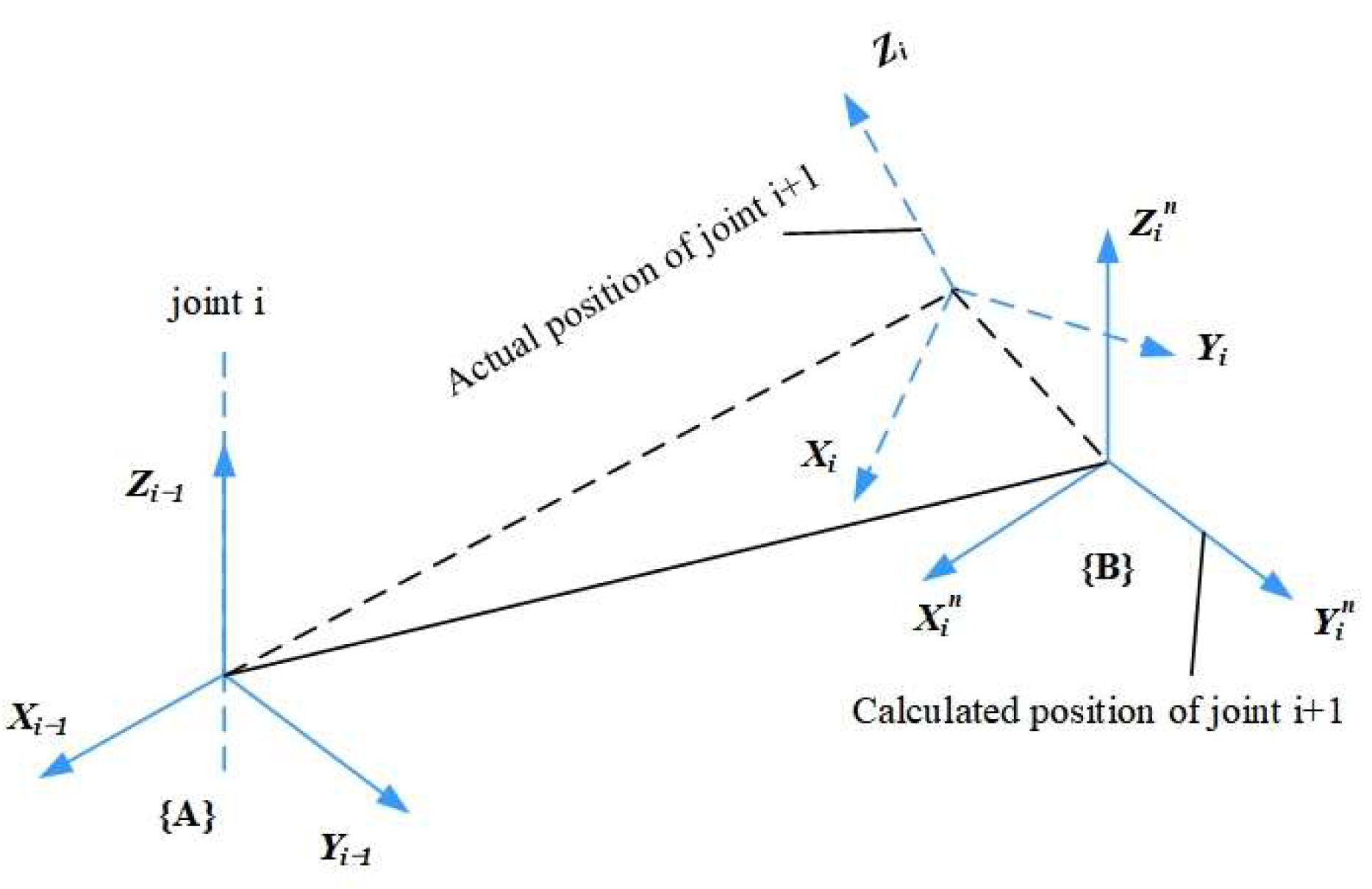
The geometric parameter errors of industrial robots mainly include joint angle error Δθi, link length error Δai, link torsion angle error Δαi, and link offset error Δdi. Among these geometric parameter errors, Δai and Δdi are errors caused by precision issues during the manufacturing, processing, and assembly of the robot’s links; Δθi is a rotational angle error caused by the zero-position error of the encoder; Δαi is an error resulting from deviations in the perpendicularity or parallelism between adjacent joint axes. An error schematic diagram of the adjacent link coordinate systems is shown in Figure 2. Kinematic parameter calibration of industrial robots is a process of compensating the end-effector pose and thereby improving the end-effector pose accuracy by identifying the errors of the above-mentioned geometric parameters.
According to Equation (4), the position error of the robot end-effector can be expressed as follows:
d T = T r T 6
where dT represents the magnitude of the position error at the end-effector of the industrial robot, Tr denotes the actual position reached by the robot end-effector, and T6 represents the theoretical position of the robot end-effector. Taking the total differentiation of dT, it can be expressed as Equation (5):
d T i = T i α i Δ α i + T i a i Δ a i + T i d i Δ d i + T i θ i Δ θ i
From Equation (5), dT is calculated jointly from the error coefficients and the four error variables Δα, Δa, Δd, and Δθ. Therefore, the error coefficient matrix can be represented using an extended Jacobian matrix, thereby deriving Equation (6):
d T = i = 1 6 J i e i = J Δ q
where J is the extended Jacobian matrix, representing the error coefficient matrix, and Δq denotes the kinematic parameter errors to be identified, including Δα, Δa, Δd, and Δθ. ei is the error generated by each joint relative to its joint coordinate system.

2.3. Optimization Problem and Fitness Function

The process of parameter identification involves solving the error equation system to obtain the kinematic parameter errors of the robot. Owing to the large number of unknown parameters in the error model, multiple sets of end-effector pose data are required to formulate the equation system for parameter identification.
F = min ( i = 1 n T R i T C i ) = min ( i = 1 n ( δ x i ) 2 + ( δ y i ) 2 + ( δ z i ) 2 )
In Equation (7), i denotes the number of target position collection points of the robot. F is a function of the geometric parameter error set (Δai, Δdi, Δαi, Δθi), serving as the fitness function for the optimization algorithm. When the industrial robot is at different positions, the error between the actual position and the theoretical position is acquired, and the true values of (Δai, Δdi, Δαi, Δθi) are solved through the optimization algorithm. The objective calculation process of the optimization algorithm aims to minimize F as much as possible, thereby reducing the actual error. Here, TRi = (xRi, yRi, zRi) represents the actual position of the collection point, and TCi = (xCi, yCi, zCi) is the theoretical position of the industrial robot calculated using the optimized kinematic parameters.

3. Robot Calibration Method Based on IGWO

3.1. Introduction to the GWO Algorithm

The GWO algorithm is a novel meta-heuristic algorithm inspired by the group predation and foraging behavior of wild grey wolves in nature. Proposed by Mirjalili et al. [32] in 2014, it optimizes the search process through the collective cooperation of the wolf pack. The wolf population is divided into four social hierarchy categories: three leading wolves α, β, δ and the remaining subordinate wolves ω, which correspond to the optimal solution and parameters to be optimized, respectively. Each grey wolf represents a potential solution, with the relative positions among wolves reflecting the quality of these solutions. Through interaction and collaboration, wolves complete the search process by surrounding, hunting, and attacking prey. The mathematical model for the “prey surrounding” behavior in the hunting process is described by Equations (8) and (9):
E = M × V p ( t ) V ( t )
V ( t + 1 ) = V p ( t ) N × E
In this context, E represents the distance between a grey wolf individual and its target prey. Vp denotes the prey’s position, while V stands for the position vector of the grey wolf, and t refers to the current iteration count. The coefficient vectors N and M are computed using Equations (10) and (11), respectively.
N = 2 × N × c 1 a ( t )
M = 2 × c 2
where c1 and c2 are random vectors with values constrained within the interval [0, 1]. Additionally, the elements of vector a undergo a linear reduction from 2 to 0 throughout the iterative process, as defined by Equation (12).
a ( t ) = 2 ( 2 × t ) / M a x I t e r
In order to mathematically formulate the hunting behavior of grey wolves, it is hypothesized that the α, β, δ wolves possess superior awareness of the prey’s location. Consequently, the remaining ω wolves are required to follow the guidance of these three top-performing individuals (α, β, δ), whose positions correspond to the optimal solutions. The mathematical description of this hunting mechanism is provided in Equations (13)–(15), where the coefficient vectors M1, M2, and M3 are derived from Equation (11).
E α = M 1 × V α V ( t ) E β = M 2 × V β V ( t ) E δ = M 3 × V δ V ( t )
V i 1 ( t ) = V α ( t ) N i 1 × E α ( t ) V i 2 ( t ) = V β ( t ) N i 2 × E β ( t ) V i 3 ( t ) = V δ ( t ) N i 3 × E δ ( t )
V ( t + 1 ) = V i 1 ( t ) + V i 2 ( t ) + V i 3 ( t ) 3
where Vα, Vβ, and Vδ stand for the three most optimal solutions at iteration t. The vectors Ni1, Ni2, and Ni3 are computed using Equation (10), while Eα, Eβ, and Eδ are defined in accordance with Equation (13). The hunting procedure comes to an end the moment the prey stops moving, which triggers the wolf pack to launch an attack. From a mathematical perspective, this shift is controlled by the parameter a. Its value drops linearly with each iteration, serving to balance exploration and exploitation. As laid out in Equation (12), a gets updated in each iteration, with its range limited to 2 to 0. According to Emary et al. [33], the iterative process is split into two equal parts: one for exploration and the other for exploitation, with a smooth transition between these two stages. At this point, each wolf changes its position to a random spot between where it currently is and the prey’s location.
When the GWO algorithm is applied to the kinematic calibration of industrial robots, it firstly generates an initial wolf pack with random positions in a large search space. This random selection method is prone to causing local optimization issues during the iteration process, thus failing to find the global optimal solution. Meanwhile, the GWO algorithm itself lacks sufficient boundary handling mechanisms, often leading to stagnation in the search for the optimal solution. Additionally, the calibration of industrial robots requires the identification of 24 kinematic parameters, which poses a severe challenge to the GWO algorithm. Therefore, to improve the robustness and accuracy of the GWO algorithm in industrial robot calibration, further improvements to the GWO algorithm are necessary.

3.2. Improvements to GWO for Kinematic Calibration

To address the issues of the GWO algorithm in industrial robot kinematic calibration, corresponding improvement strategies have been proposed. These improvements mainly involve new search strategies applied in three stages: initialization, movement, and selection–update.
(1)
Improvements to the initialization phase.
Since the GWO algorithm generates an initial wolf pack with random positions during the initialization stage, the algorithm often fails to find the global optimal solution in the iterative process. Therefore, the positions of the wolf pack are rearranged in the initialization stage by selecting random wolves with lower fitness values and eliminating those with excessively high fitness values.
During this phase, a total of W grey wolves are randomly placed within the search space, with their positions bounded by the given range [yi, zj] as specified by Equation (16). For the i-th grey wolf in iteration t, its location is characterized as a real-valued vector Vi(t) = {vi1, vi2, ..., viP}. p signifies the dimensional attribute of the optimization task. The entire wolf population is stored in a matrix Pop, featuring L rows and p columns. To determine the fitness of Vi(t), the fitness function f(Vi(t)) is employed for calculation.
V i j = y i + r a n d j 0 , 1 × ( z j y i ) , i 1 , L , j 1 , P
In Equation (16), yi and zj represent the lower bound and upper bound of the j-th dimensional variable in the search space, respectively. They define the value range [yi, zj] for variables in each dimension, which functions to constrain the initial position distribution of grey wolves and ensure they are within a reasonable solution space. Vij indicates the position coordinate of the i-th grey wolf in the j-th dimension.
(2)
Improvements to the boundary-processing strategy.
Beyond synchronized group hunting, solitary predation stands out as another notable social characteristic in grey wolves, forming the cornerstone for our proposed adjustments to the GWO. The IGWO incorporates an additional movement protocol known as the DL search strategy. Within the DL structure, each wolf is regarded by its adjacent peers as a substitute candidate solution during the update of Vi(t)’s new position. The following steps elaborate on how the traditional GWO and DL search strategies generate two separate candidate solutions.
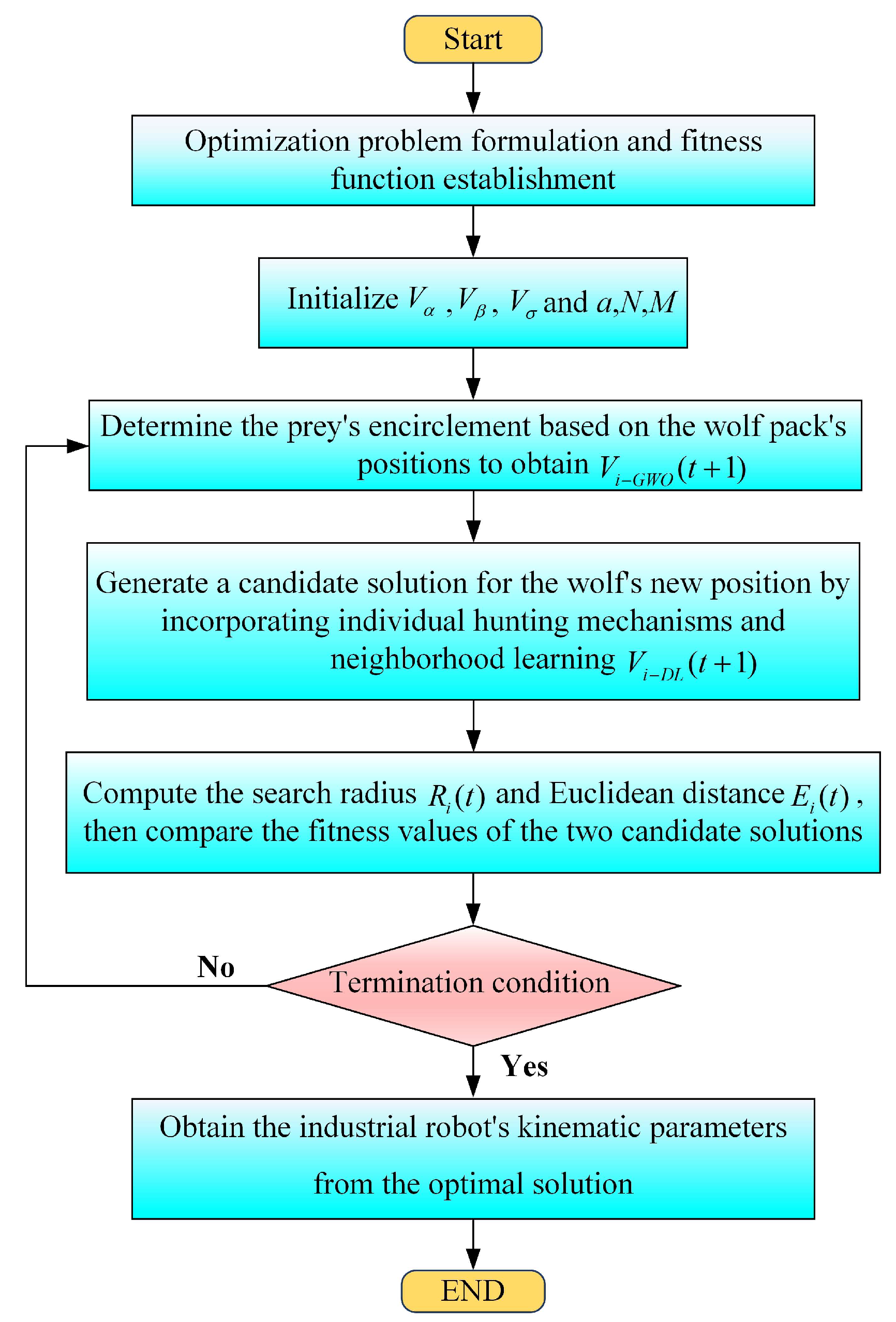
In the standard GWO search mechanism, as discussed previously, the three highest-performing wolves within the Pop matrix are designated as α, β, and δ. Following this, the linearly diminishing coefficient a, together with coefficients N and M, are computed using Equations (10)–(12). Subsequently, the encirclement area of the prey is determined by incorporating the positions of Vα, Vβ, and Vδ through Equations (13) and (14). Lastly, the initial candidate solution for the new position of wolf Vi(t), denoted as ViGWO(t + 1), is derived using Equation (15).
In the standard GWO, each wolf produces a new position with the support of the three dominant wolves in the population. This method results in the slow convergence of the algorithm, the early depletion of population diversity, and a tendency for the wolf pack to become stuck in local optima. To mitigate these limitations, the proposed DL search strategy integrates the individual hunting behavior of wolves, where such behavior is learned from their neighboring individuals.
Within the DL search strategy, each dimension of the new position for wolf Vi(t) is computed using Equation (19). In this progress, the wolf gains insights from a range of adjacent individuals and a randomly chosen wolf within the population matrix Pop. Apart from the standard updated position ViGWO(t + 1), the DL strategy produces an additional candidate solution for the new position of Vi(t), known as ViDL(t + 1). To accomplish this, the radius Ri(t) is initially computed through the Euclidean distance between the current position of Vi(t) and the candidate position ViGWO(t + 1), as stated by equation (17). Next, the neighbors of Vi(t), referred to as Si(t), are generated using Equation (18) with reference to the radius Ri(t). Ei(t) represents the Euclidean distance between Vi(t) and Vj(t).
R i ( t ) = V i ( t ) V i G W O ( t + 1 )
S i ( t ) = V j ( t ) | E i V i t , V j t R i ( t ) , V j ( t ) P o p
After the neighbor set of Vi(t) is determined, multi-neighbors learning is carried out with the use of Equation (19). In this equation, the d-th dimension of ViDL(t + 1) is computed by integrating the d-th dimension of a randomly picked neighbor Vn,d(t) from Si(t) and the d-th dimension of a randomly chosen wolf Vr,d(t) from the population matrix Pop.
V i D L , d ( t + 1 ) = V i , d ( t ) + r a n d × V n , d ( t ) V r , d ( t )
(3)
Improvements to parameters update strategy.
In this phase, the winning candidate solution is first selected by comparing the fitness values of the two candidates ViGWO(t + 1) and ViDL(t + 1) using Equation (20).
V i ( t + 1 ) = V i G W O ( t + 1 )   , i f   f ( V i G W O ) < f ( V i D L )   V i D L ( t + 1 ) o t h e r w i s e
Subsequently, when updating the position of Vi(t + 1), a comparison is made between the fitness value of the chosen candidate solution and that of Vi(t). If the former is lower, Vi(t) is substituted with this optimal candidate; otherwise, Vi(t) retains its original position in the population matrix Pop. Eventually, once this operation is applied to every individual in the pack, the iteration counter (iter) is incremented by 1, and the search process repeats until it reaches the maximum number of iterations (Maxiter).
To clearly describe the application of the IGWO algorithm in the kinematic calibration of industrial robots, the process is illustrated in Figure 3. The algorithm first randomly generates an initial wolf pack within the search space and evaluates the positions of the wolves based on the fitness function. In each iteration, the top three wolves with the best fitness values are identified as α, β, and δ. Thereafter, each wolf updates its position according to the aforementioned steps to encircle, hunt, and attack the prey. Finally, by repeating these steps, the optimal position of the prey is determined. Specifically, the position of α can be found, until the termination criteria are met, which include achieving a sufficiently good fitness value or reaching the preset maximum number of iterations. In this context, a sufficiently good fitness value indicates that the calculated error value F is less than the preset error value.

4. Error Compensation Experiment

The experimental object of this paper is an automated assembly system with the ABB IRB4600 industrial robot as its core component. This section aims to verify the effectiveness of the IGWO algorithm primarily through experiments on the kinematic error compensation and calibration of industrial robots. Additionally, a comparison will be made between the IGWO algorithm and other algorithms, including the LM algorithm, Genetic Algorithm (GA), and PSO algorithm, in terms of their calibration effects on robot kinematic parameters. Meanwhile, the calibration experiment of industrial robots requires the identification of 24 kinematic parameters. When the GWO algorithm is applied to the kinematic parameter identification of industrial robots, it often suffers from low search efficiency. For instance, it may take hundreds of iterations to find the optimal solution. Moreover, due to the inherent limitations in GWO’s search mechanism, issues such as failure to converge to the optimal solution or significant deviation between the found optimal solution and the true value (resulting in invalid solutions) may arise during the iteration process. This indicates that the GWO algorithm exhibits low computational efficiency and weak robustness in the kinematic parameter identification of industrial robots, failing to meet our requirements for industrial robot parameter identification. Therefore, this paper will not compare the GWO algorithm with other algorithms.

4.1. Experimental Instruments

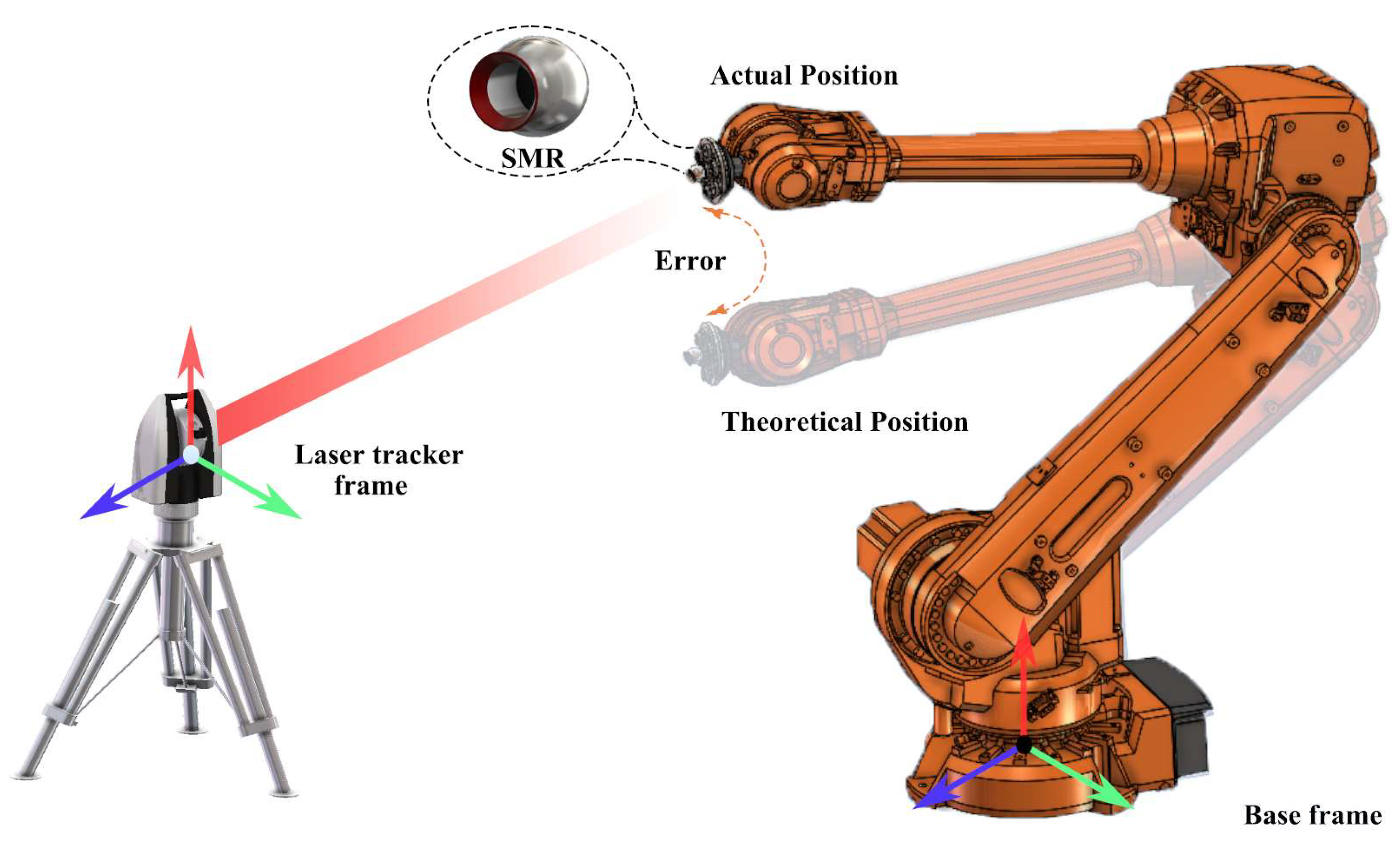
According to the error model of industrial robots established in Section 2.2, the kinematic parameters to be calibrated can be obtained. The accuracy of these parameters can be verified by identifying them and performing error compensation. The theoretical position can be calculated by the robot kinematic model, while the actual position is measured by instruments. Figure 4 shows the theoretical model diagram of the calibration experiment.
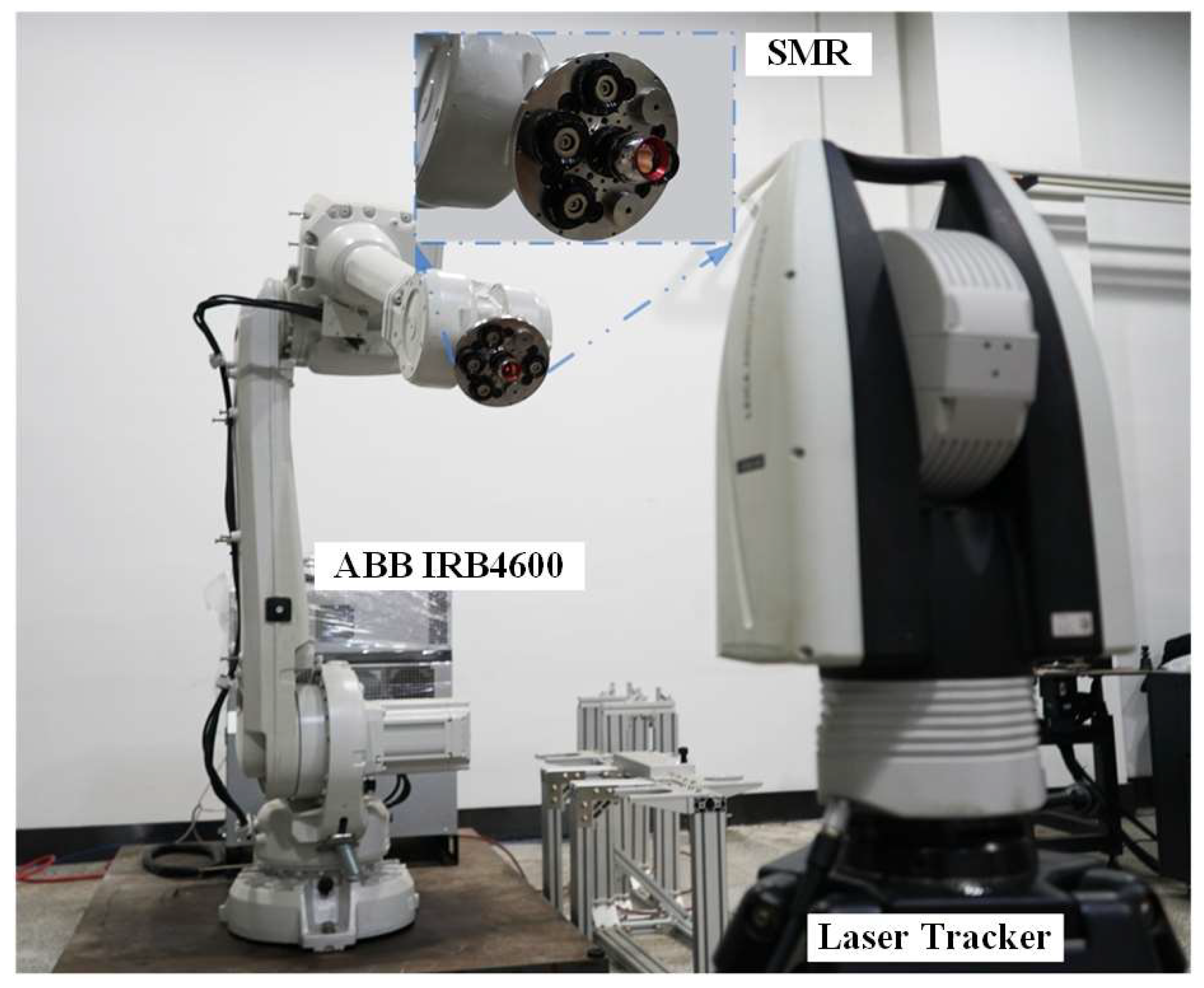
Figure 5 shows the experimental system used to verify the effectiveness of the proposed IGWO algorithm in calibrating industrial robots. The drilling and riveting robot system mainly consists of an ABB IRB4600 robot with a payload of 40 kg and a repeatability of ±0.06 mm. The laser tracker used in this experiment is the Leica-AT960-MR model, a portable dynamic 6DOF laser measurement system manufactured by Hexagon Metrology GmbH in Wetzlar, Germany. This instrument features high measurement accuracy, reaching 15 μm ± 6 μm/m. The tracking target of the laser tracker is a Leica 1.5-inch spherically mounted reflector (SMR) detectable by the laser tracker, which can be installed on the adapter plate at the robot’s end-effector with a maximum measurement distance of 20 m. The base coordinate system of the laser tracker is established using SpatialAnalyzer (SA) software. SA is a professional grade 3D measurement and analysis software developed by New River Kinematics, a U.S. company. With this software, geometric features such as circles and planes can be easily fitted using the collected spatial points. Additionally, this software allows for convenient coordinate system construction, enabling any coordinate system to be set as the current measurement coordinate system. When the constructed robot base coordinate system is set as the current measurement coordinate system, the actual position coordinates of the collected points relative to the robot’s base coordinate system can be easily obtained. Meanwhile, the position of the robot’s base coordinate system must be consistent with the system coordinate system of the laser tracker’s measurement software.

4.2. Experimental Setup

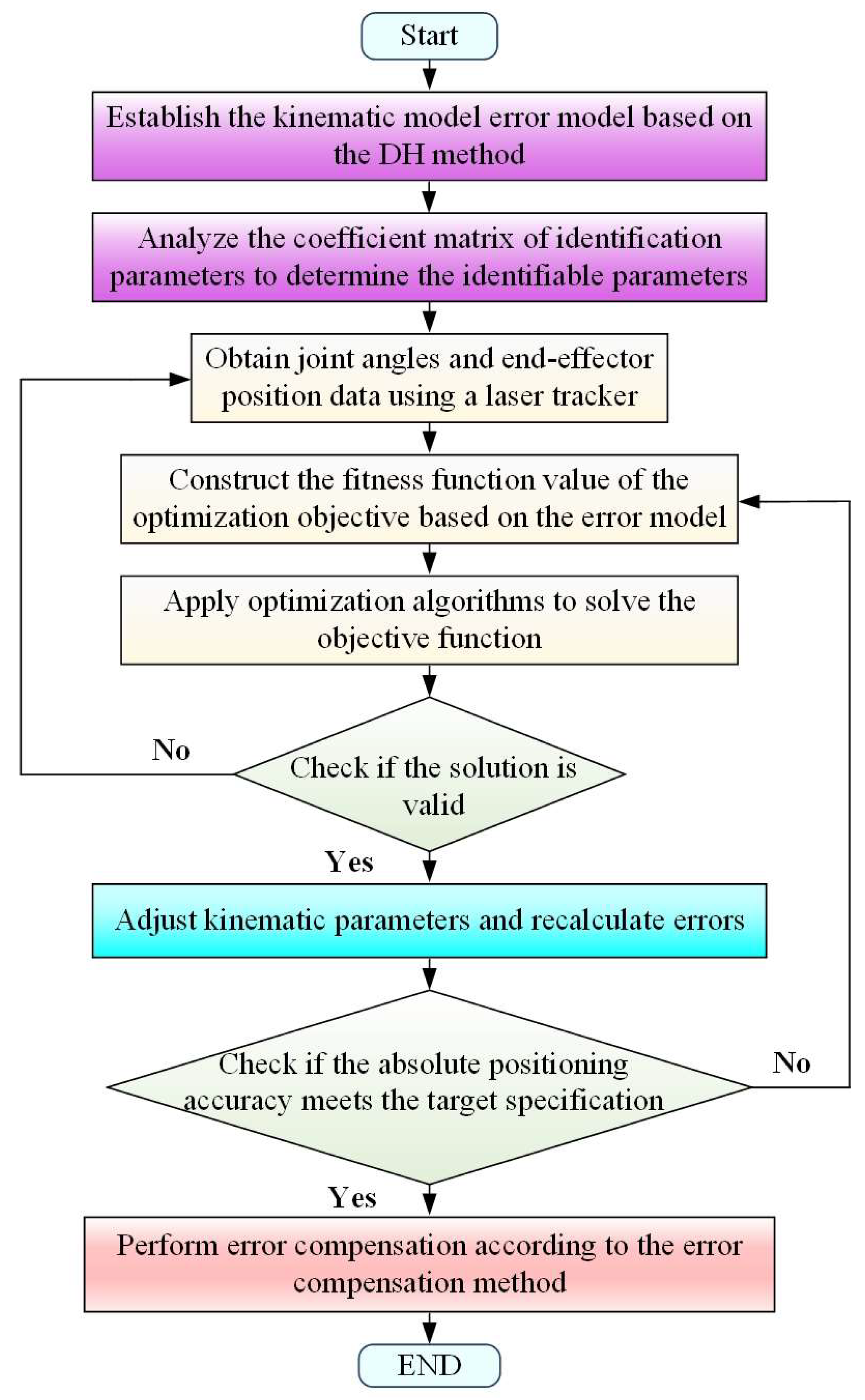
Figure 6 shows the calibration process. Since the robot has six degrees of freedom, a total of 24 DH parameters need to be determined. Firstly, the kinematic model and end-effector position error model of the robot are established based on the kinematic parameters of the ABB IRB4600 industrial robot. The laser tracker is used to measure the end-effector position of the robot, calculate the position error, and record the corresponding robot joint angles. Then, optimization methods are employed to identify the errors in the kinematic parameters. When using optimization algorithms, invalid solutions may occasionally arise. Therefore, it is necessary to check the validity of these obtained parameter error solutions. Finally, based on these error data, position compensation is performed on the robot to improve the end-effector positioning accuracy. Theoretically, the more positions provided, the higher the accuracy of parameter determination.
In industrial robotics, the base coordinate system of a robot is typically located at the center of the robot’s bottom mounting surface, but its exact position is difficult to measure directly. Therefore, during the experiment, the correlation between the base coordinate system, measurement coordinate system, flange coordinate system, and end-effector coordinate system was first established. After completing the establishment of the flange coordinate system and base coordinate system, according to the calibration process given earlier, the collection of end-position points began.
In the industrial robot controller, 150 robot pose coordinate points were predefined as the theoretical positions of the robot, and these 150 points were distributed as evenly as possible throughout the robot’s entire workspace. A 3 s waiting time was set between each motion command in the program to facilitate position measurement by the laser tracker. The robot was then controlled to move at 100% speed. When the robot reached the given target position, it paused for 3 s. During this time, the theoretical sampling point positions measured by the laser tracker, the corresponding joint angles of the robot, and the actual sampling point positions were recorded.

4.3. Parameter Identification

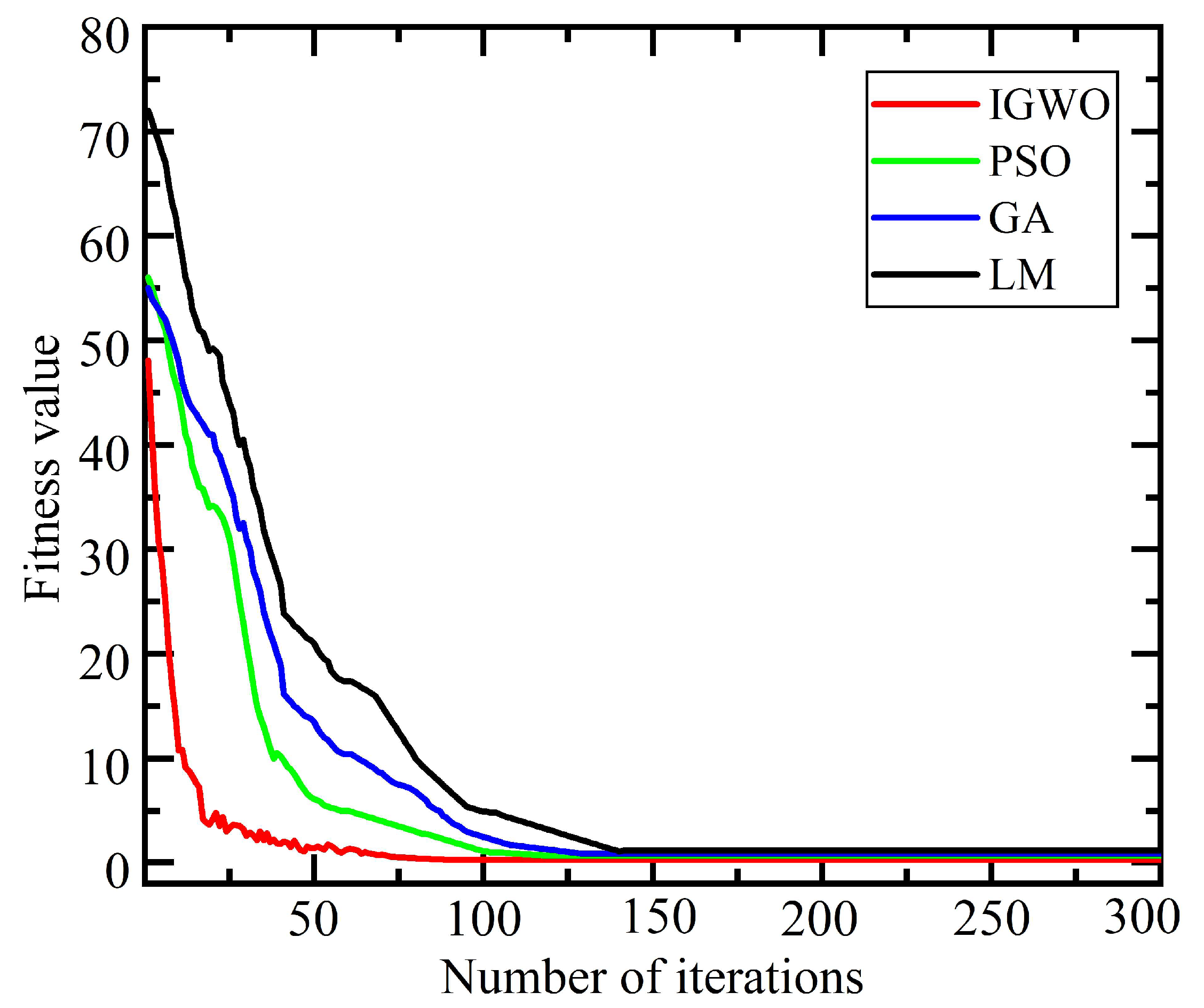
After completing the measurement of sampling points, the LM, PSO, GA, and IGWO algorithms were used to identify the kinematic parameters of the industrial robot. The calculation process was repeated 30 times, and the average change curve of the fitness function values during the solution process is shown in Figure 7. Figure 7 depicts the trend curves of the fitness function values for these four algorithms, where the abscissa represents the number of iterations of the algorithm, and the ordinate represents the fitness function obtained during the iteration process.
Figure 7 shows that the LM algorithm achieved the best fitness function value of 1.132 after 145 iterations. The GA and PSO algorithms obtained the best fitness function values of 0.847 and 0.685 after 134 and 126 iterations, respectively. In contrast, the IGWO algorithm obtained the best fitness function value of 0.452 after only 95 iterations. Compared with other optimization methods, the IGWO algorithm demonstrates faster convergence speed and superior fitness function values. Furthermore, due to the adoption of the DL search strategy, the IGWO algorithm can converge more rapidly in the initial stage, effectively reducing the calculation time of the algorithm.
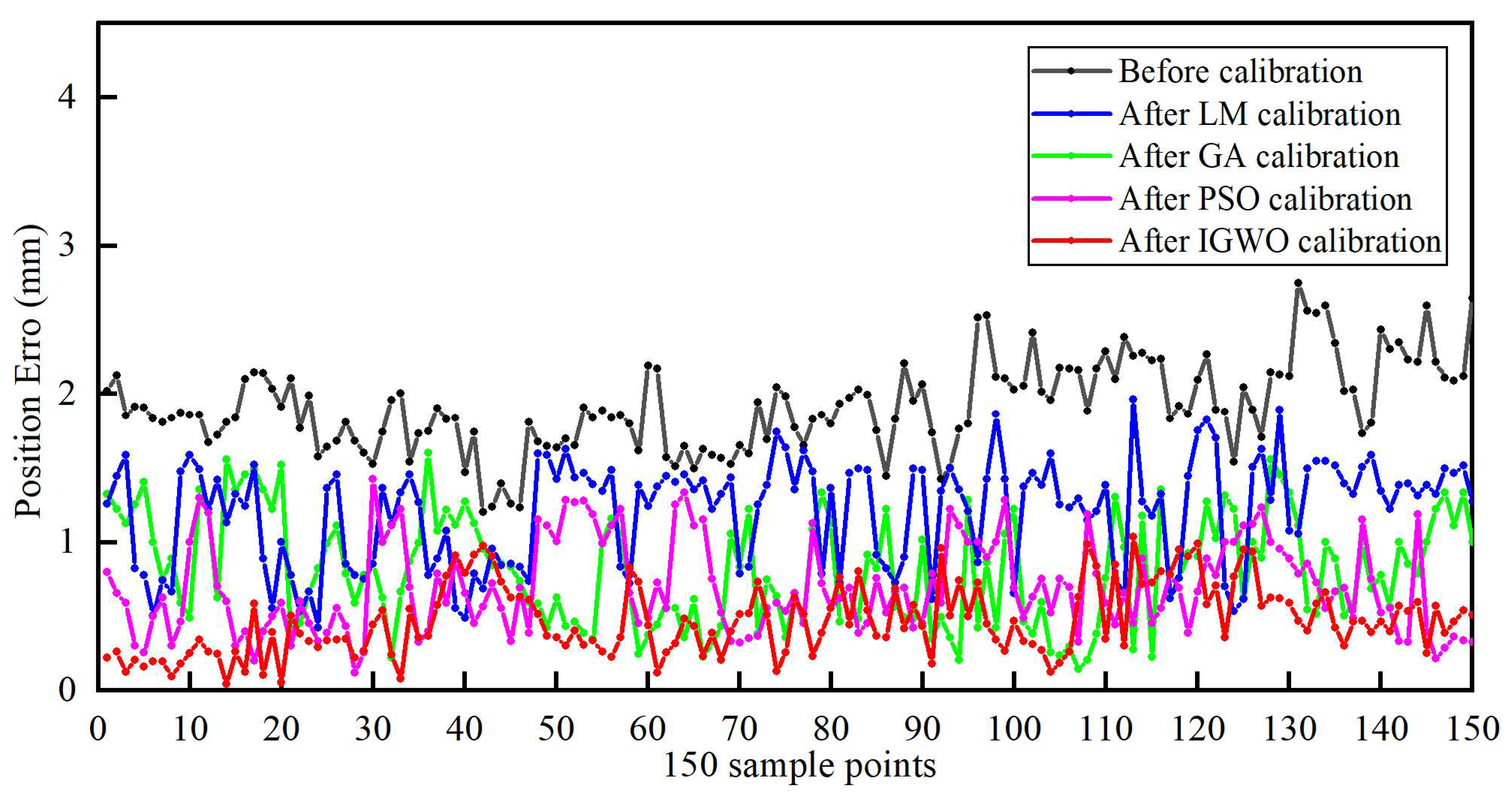
After obtaining four sets of different kinematic parameters for the industrial robot, error parameter compensation was performed, and the position error of each of the 150 initially collected sampling points was compared before and after compensation. Table 2 presents the kinematic parameters of the industrial robot calculated using the IGWO algorithm. Figure 8 illustrates the position error data of the robot before and after compensation using the four optimization algorithms.
From the compensation results, it can be observed that after compensating the 150 collected points of the industrial robot, all four algorithms, IGWO, PSO, GA, and LM, improved the calibrated positioning accuracy. Specifically, the average positioning errors were reduced from 1.935 mm to 0.471 mm (IGWO), 0.697 mm (PSO), 0.868 mm (GA), and 1.207 mm (LM), respectively. Although all four algorithms enhance the robot’s positioning accuracy, the IGWO algorithm demonstrates faster convergence and yields more effective compensation results.

4.4. Error Compensation Verification

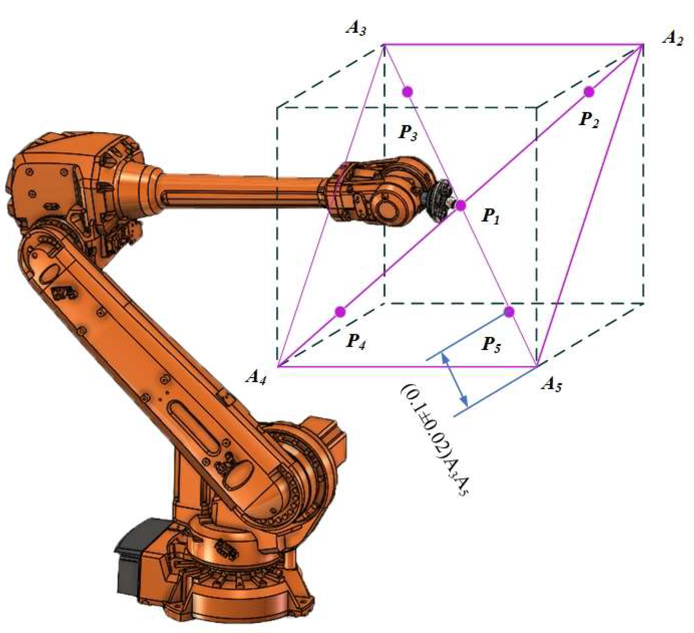
To validate the calibration effectiveness of this experiment at other positions within the robot’s workspace, the calibration results were verified in accordance with the industrial robot position accuracy detection method specified in GB/T 12642-2013 [34] “Industrial robots—Performance criteria and related test methods”. As illustrated in Figure 9, within the industrial robot controller, a cubic region most frequently utilized in robot applications was selected according to the robot performance verification protocol, and the positions of five test points were calculated. A program was then developed to instruct the robot to cycle 30 times in the sequence of P1P2P3P4P5, with a laser tracker employed to measure the actual positions of these points.
Error compensation was performed on the five test points based on the identified parameter errors. The robot was subsequently controlled to execute another 30 cycles of motion, and the laser tracker was used to measure the actual positions of the compensated test points. Table 3 lists the average values (Mean), maximum values (Max), and standard deviations (STD) of the robot position errors for 150 test points at five positions before and after calibration using the four optimization algorithms.
Table 3 shows that the absolute positioning accuracy of the industrial robot before calibration is 1.918 mm. Using LM, GA, and PSO, the accuracy can be reduced to 1.194 mm, 0.845 mm, and 0.672 mm, respectively, while using IGWO can reduce it to 0.475 mm. Therefore, the kinematic calibration based on the IGWO algorithm is more accurate and effective than the other three methods.

5. Conclusions

To address the issue that industrial robots fail to meet precision requirements during the drilling and riveting of large-scale components like aircraft parts due to insufficient absolute positioning accuracy, this study proposes a kinematic calibration method for industrial robots based on the IGWO algorithm, aiming to enhance their absolute positioning accuracy. Firstly, the kinematic model and the error model of typical industrial robots were established. Then, the kinematic parameters to be optimized in the calibration process were determined, and these parameters were used to calculate the target fitness function to be solved. Secondly, leveraging the established robot kinematic error model, a novel IGWO-based kinematic calibration method was developed. By integrating a DL search strategy into the traditional GWO algorithm, the stability and optimization performance of the algorithm were significantly enhanced. Next, the effectiveness of the IGWO algorithm was verified through kinematic error compensation and calibration experiments. Using an ABB IRB4600 industrial robot as the test subject, the proposed IGWO algorithm was applied for kinematic parameter identification, and its calibration performance was compared with that of other traditional optimization algorithms. Calibration experiments were conducted using a laser tracker, and the results demonstrated that the absolute positioning accuracy of the industrial robot was ultimately improved from 1.918 mm to 0.475 mm. Overall, this method resolves the long-standing issue where low absolute positioning accuracy hinders industrial robots from meeting processing requirements in high-precision industrial fields. Additionally, it overcomes the inherent limitations of the traditional GWO algorithm, such as convergence stagnation and vulnerability to local optima during computation. As a result, it provides a high-precision and robust calibration solution for industrial robots.

Author Contributions

All authors contributed to this work. Conceptualization: B.C. and L.W.; methodology: B.C. and J.Y.; software: B.C., Y.Z. (Yi Zhang) and P.L.; validation: B.C., Y.Z. (Yifan Zhang) and H.S.; investigation: B.C. and L.W.; resources: L.W., P.J. and J.L.; writing—original draft preparation: B.C.; writing—review and editing: B.C. and L.W.; visualization: B.C. All authors have read and agreed to the published version of the manuscript.

Funding

This research received no external funding.

Data Availability Statement

The data that support the findings of this study are available on request from the corresponding author. The data are not publicly available due to privacy and ethical restrictions.

Conflicts of Interest

The authors declare no conflicts of interest.

References

  1. Zhang, L.; Gao, W.; Lu, D.; Zeng, D.; Lei, P.; Yu, J.; Tang, M. Robotic simple and fast drilling system for automated aircraft assembly. Int. J. Adv. Manuf. Technol. 2022, 122, 411–426. [Google Scholar] [CrossRef]
  2. Ma, F.; Cao, W.; Luo, Y.; Qiu, Y. The review of manufacturing technology for aircraft structural part. Procedia CIRP 2016, 56, 594–598. [Google Scholar] [CrossRef][Green Version]
  3. Frommknecht, A.; Kuehnle, J.; Effenberger, I.; Pidan, S. Multi-sensor measurement system for robotic drilling. Robot. Comput. Integr. Manuf. 2017, 47, 4–10. [Google Scholar] [CrossRef]
  4. Liu, Y.; Zhuang, Z.; Li, Y. Closed-loop kinematic calibration of robots using a six-point measuring device. IEEE Trans. Instrum. Meas. 2022, 71, 1–12. [Google Scholar] [CrossRef]
  5. Lin, Y.; Zhao, H.; Ding, H. Spindle configuration analysis and optimization considering the deformation in robotic machining applications. Robot. Comput. Integr. Manuf. 2018, 54, 83–95. [Google Scholar] [CrossRef]
  6. Olsson, T.; Haage, M.; Kihlman, H.; Johansson, R.; Nilsson, K.; Robertsson, A.; Brogardh, T. Cost-efficient drilling using industrial robots with high-bandwidth force feedback. Robot. Comput. Integr. Manuf. 2010, 26, 24–38. [Google Scholar] [CrossRef]
  7. Xu, H.; Xue, J.; Guo, G.; Liu, Y.; Liu, M.; Zhang, D. Stiffness optimization of a robotic drilling system for enhanced accuracy in aerospace assembly. Actuators 2025, 14, 86. [Google Scholar] [CrossRef]
  8. Li, Z.; Tian, W.; Wang, M.; Li, B.; Liao, W. Positioning error compensation of a flexible track hybrid robot for aircraft assembly based on response surface methodology and experimental study. Int. J. Adv. Manuf. Technol. 2022, 119, 1313–1330. [Google Scholar] [CrossRef]
  9. Ma, S.; Deng, K.; Lu, Y.; Xu, X. Robot error compensation based on incremental extreme learning machines and an improved sparrow search algorithm. Int. J. Adv. Manuf. Technol. 2023, 125, 5431–5443. [Google Scholar] [CrossRef]
  10. Lattanzi, L.; Cristalli, C.; Massa, D.; Boria, S.; Lépine, P.; Pellicciari, M. Geometrical calibration of a 6-axis robotic arm for high accuracy manufacturing task. Int. J. Adv. Manuf. Technol. 2020, 111, 1813–1829. [Google Scholar] [CrossRef]
  11. Nubiola, A.; Bonev, I.A. Absolute calibration of an ABB IRB 1600 robot using a laser tracker. Robot. Comput. Integr. Manuf. 2013, 29, 236–245. [Google Scholar] [CrossRef]
  12. Le, P.N.; Kang, H.J. Robot manipulator calibration using a model based identification technique and a neural network with the teaching learning-based optimization. IEEE Access 2020, 8, 105447–105454. [Google Scholar] [CrossRef]
  13. Roth, Z.; Mooring, B.; Ravani, B. An overview of robot calibration. IEEE J. Robot. Autom. 2003, 3, 377–385. [Google Scholar] [CrossRef]
  14. Kim, S.H.; Nam, E.; Ha, T.I.; Hwang, S.H.; Lee, J.H.; Park, S.H.; Min, B.K. Robotic machining: A review of recent progress. Int. J. Precis. Eng. Manuf. 2019, 20, 1629–1642. [Google Scholar] [CrossRef]
  15. Jiang, Z.; Zhou, W.; Li, H.; Mo, Y.; Ni, W.; Huang, Q. A new kind of accurate calibration method for robotic kinematic parameters based on the extended Kalman and particle filter algorithm. IEEE Trans. Ind. Electron. 2017, 65, 3337–3345. [Google Scholar] [CrossRef]
  16. Gao, G.; Liu, F.; San, H.; Wu, X.; Wang, W. Hybrid Optimal Kinematic Parameter Identification for an Industrial Robot Based on BPNN-PSO. Complexity 2018, 1, 4258676. [Google Scholar] [CrossRef]
  17. Luo, G.; Zou, L.; Wang, Z.; Lv, C.; Ou, J.; Huang, Y. A novel kinematic parameters calibration method for industrial robot based on Levenberg-Marquardt and Differential Evolution hybrid algorithm. Robot. Comput. Integr. Manuf. 2021, 71, 102165. [Google Scholar] [CrossRef]
  18. Zhong, H.; Hu, C.; Li, X.; Gao, L.; Zeng, B.; Dong, H. Kinematic calibration method for a two-segment hydraulic leg based on an improved whale swarm algorithm. Robot. Comput. Integr. Manuf. 2019, 59, 361–372. [Google Scholar] [CrossRef]
  19. Li, Z.; Li, S.; Luo, X. Using quadratic interpolated beetle antennae search to enhance robot arm calibration accuracy. IEEE Robot. Autom. Lett. 2022, 7, 12046–12053. [Google Scholar] [CrossRef]
  20. Chen, X.; Zhan, Q. The kinematic calibration of an industrial robot with an improved beetle swarm optimization algorithm. IEEE Robot. Autom. Lett. 2022, 7, 4694–4701. [Google Scholar] [CrossRef]
  21. Zak, G.; Benhabib, B.; Fenton, R.G.; Saban, I. Application of the weighted least squares parameter estimation method to the robot calibration. J. Mech. Des. 1994, 116, 890–893. [Google Scholar] [CrossRef]
  22. Nadimi-Shahraki, M.H.; Taghian, S.; Mirjalili, S. An improved grey wolf optimizer for solving engineering problems. Expert Syst. Appl. 2021, 166, 113917. [Google Scholar] [CrossRef]
  23. Messay, T.; Ordóñez, R.; Marcil, E. Computationally efficient and robust kinematic calibration methodologies and their application to industrial robots. Robot. Comput. Integr. Manuf. 2016, 37, 33–48. [Google Scholar] [CrossRef]
  24. Theissen, N.A.; Laspas, T.; Archenti, A. Closed-force-loop elastostatic calibration of serial articulated robots. Robot. Comput. Integr. Manuf. 2019, 57, 86–91. [Google Scholar] [CrossRef]
  25. Dehghani, M.; McKenzie, R.A.; Irani, R.A.; Ahmadi, M. Robot-mounted sensing and local calibration for high-accuracy manufacturing. Robot. Comput. Integr. Manuf. 2023, 79, 102429. [Google Scholar] [CrossRef]
  26. Nubiola, A.; Slamani, M.; Joubair, A.; Bonev, I.A. Comparison of two calibration methods for a small industrial robot based on an optical CMM and a laser tracker. Robotica 2014, 32, 447–466. [Google Scholar] [CrossRef]
  27. Du, G.; Liang, Y.; Li, C.; Liu, P.X.; Li, D. Online robot kinematic calibration using hybrid filter with multiple sensors. IEEE Trans. Instrum. Meas. 2020, 69, 7092–7107. [Google Scholar] [CrossRef]
  28. Zhao, G.; Zhang, P.; Ma, G.; Xiao, W. System identification of the nonlinear residual errors of an industrial robot using massive measurements. Robot. Comput. Integr. Manuf. 2019, 59, 104–114. [Google Scholar] [CrossRef]
  29. Liu, F.; Gao, G.; Na, J.; Zhang, F. L2-Regularization-Based kinematic parameter identification for industrial robots in limited measurement space. Actuators 2025, 14, 144. [Google Scholar] [CrossRef]
  30. Sun, Y.; Lu, L.; Wu, F.; Xiao, S.; Sha, J.; Zhang, L. Error analysis of a coordinate measuring machine with a 6-DOF industrial robot holding the probe. Actuators 2023, 12, 173. [Google Scholar] [CrossRef]
  31. Szabo, R.; Ricman, R.S. Robotic arm position computing method in the 2d and 3d spaces. Actuators 2023, 12, 112. [Google Scholar] [CrossRef]
  32. Mirjalili, S.; Mirjalili, S.M.; Lewis, A. Grey wolf optimizer. Adv. Eng. Softw. 2014, 69, 46–61. [Google Scholar] [CrossRef]
  33. Emary, E.; Zawbaa, H.M.; Grosan, C. Experienced gray wolf optimization through reinforcement learning and neural networks. IEEE Trans. Neural Netw. Learn. Syst. 2017, 29, 681–694. [Google Scholar] [CrossRef] [PubMed]
  34. Industrial Robots—Performance Criteria and Related Test Methods. Available online: https://openstd.samr.gov.cn/bzgk/gb/newGbInfo?hcno=713D24CC6BC709694DC90BADA7EE9014 (accessed on 12 November 2013).
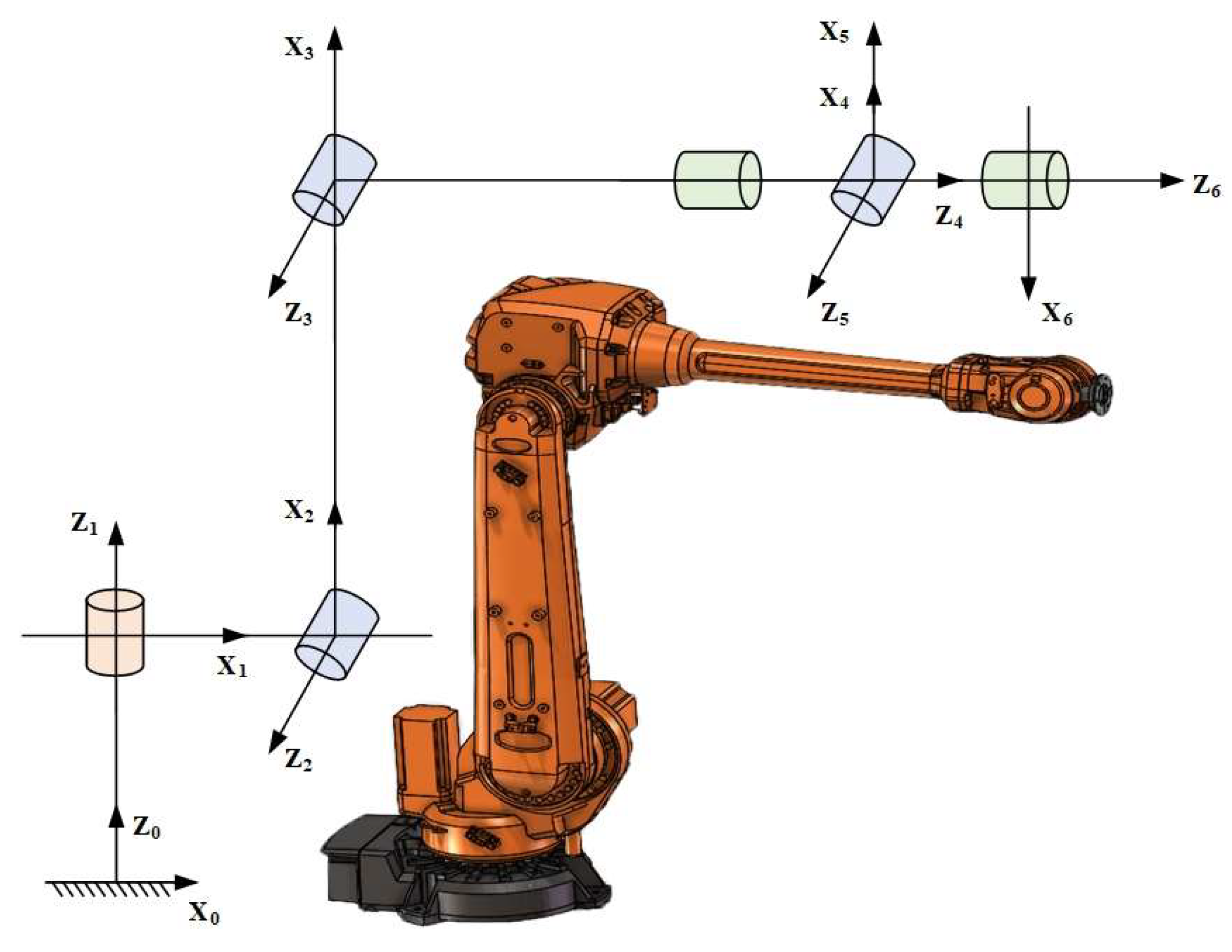
Figure 1. Kinematic model of ABB IRB4600.
Actuators 14 00403 g001
Figure 2. Schematic diagram of joint link parameter errors.
Actuators 14 00403 g002
Figure 3. IGWO algorithm application flowchart in industrial robot calibration.
Actuators 14 00403 g003
Figure 4. Theoretical model diagram of robot calibration experiment.
Actuators 14 00403 g004
Figure 5. Robot calibration experimental system.
Actuators 14 00403 g005
Figure 6. Robot kinematic parameter calibration procedure.
Actuators 14 00403 g006
Figure 7. Search processes of IGWO, PSO, GA, and LM algorithms.
Actuators 14 00403 g007
Figure 8. The comparison of sample point positioning errors after calibration.
Actuators 14 00403 g008
Figure 9. Industrial robot absolute positioning accuracy detection.
Actuators 14 00403 g009
Table 1. Theoretical DH parameters of ABB IRB4600.
Joint iαi (°)ai (mm)di (mm)θi (°)
1−901754950
2010950−90
3−9017500
490012700
5−90000
6001350
Table 2. DH parameters of ABB IRB4600 after calibration by using the IGWO algorithm.
Joint iαi (rad)ai (mm)di (mm)θi (rad)
1−0.4999174.95494.95−0.0001
20.00031094.9628−0.0499−0.4999
3−0.5001174.9509−0.04980.0002
40.4996−0.051269.95010.0007
5−0.4993−0.049−0.04890.0001
6−0.049−0.051134.9566−0.0476
Table 3. Comparison of calibration results of four optimization algorithms.
Position Errors (mm)MeanMaxSTD
Before calibration1.9182.7470.348
After calibrationLM1.1941.9650.286
GA0.8451.6320.245
PSO0.6721.4230.197
IGWO0.4751.0350.153
Disclaimer/Publisher’s Note: The statements, opinions and data contained in all publications are solely those of the individual author(s) and contributor(s) and not of MDPI and/or the editor(s). MDPI and/or the editor(s) disclaim responsibility for any injury to people or property resulting from any ideas, methods, instructions or products referred to in the content.