Autonomous Swing Motion Planning and Control for the Unloading Process of Electric Rope Shovels

Abstract

Electric rope shovels play a critical role in open-pit mining, where their automation and operational efficiency directly affect productivity. This paper presents a LiDAR-based relative positioning method to determine the spatial relationship between the ERS and mining trucks. The method utilizes dynamic DBSCAN for noise removal and RANSAC for truck edge detection, enabling robust and accurate localization. Leveraging this positioning data, a time-optimal trajectory planning strategy is proposed specifically for autonomous swing motion during the unloading process. The planner incorporates velocity and acceleration constraints to ensure smooth and efficient movement, while obstacle avoidance mechanisms are introduced to enhance safety in constrained excavation environments. To execute the planned trajectory with high precision, a neural network-based sliding-mode controller is designed. An adaptive RBF network is integrated to improve adaptability to model uncertainties and external disturbances. Experimental results on a scaled-down prototype validate the effectiveness of the proposed positioning, planning, and control strategies in enabling accurate and autonomous swing operation for efficient unloading.

1. Introduction

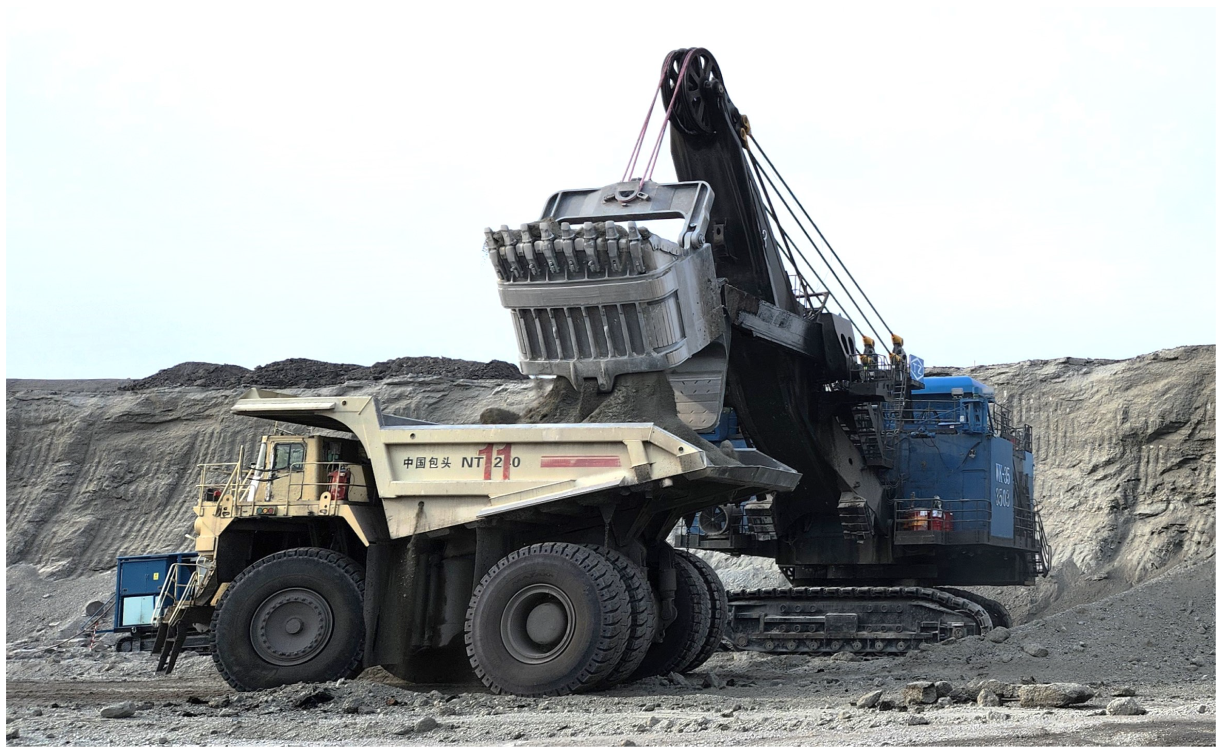
Open-pit mining [1,2] is a cornerstone of the global mineral extraction industry, and electric rope shovels (ERSs), shown in Figure 1, play a crucial role in large-scale mining operations. The ERS, featuring large-scale mechanical structures, including the boom, dipper, swing, and hoist systems, significantly impacts overall mining efficiency, energy consumption, and operational costs. Given its importance, improving the automation [3] and intelligence [4] of ERS operations has become a pressing research focus in modern mining technology.

With the advent of automation and smart mining systems [5,6,7,8], there is an increasing need for autonomous excavation technology to enhance the efficiency, safety, and adaptability of ERS operations. Automated excavation offers substantial benefits, such as reducing reliance on human operators, minimizing operational inconsistencies, and improving energy efficiency [9]. However, realizing autonomous excavation requires two fundamental aspects: precise trajectory planning and robust motion control. These aspects ensure that the excavation process is efficient, adaptable to varying material properties, and resilient to environmental disturbances.

Trajectory planning [10] in mining shovels has been extensively studied, with researchers developing various optimization-based and data-driven methods to generate efficient excavation paths. Recent advancements include digital twin-based trajectory generation, multi-objective excavation optimization [11,12], and real-time task-oriented digging trajectory planning [13]. These methods aim to enhance excavation efficiency, minimize energy consumption, and optimize digging impact [14,15,16]. Moreover, motion control strategies [17,18] have also evolved significantly [19], incorporating techniques such as nonlinear controllers [20], impedance control [21], model predictive control [22], and sliding-mode control to ensure precise and stable shovel operations despite external disturbances.

Current research primarily focuses on trajectory planning for material excavation. Recent works have also explored autonomous operation of electric rope shovels. For instance, Ref. [23] evaluated various levels of shovel automation through discrete event simulation, demonstrating up to 41% productivity improvement. In contrast, Ref. [24] focused on automating the digging phase using path planning and stall detection, validated on a scaled prototype. While these studies provide valuable insights into excavation automation, the coordination between the ERS and the mining truck during the swing unloading process, especially in terms of integrated trajectory planning and control, remains largely underexplored.

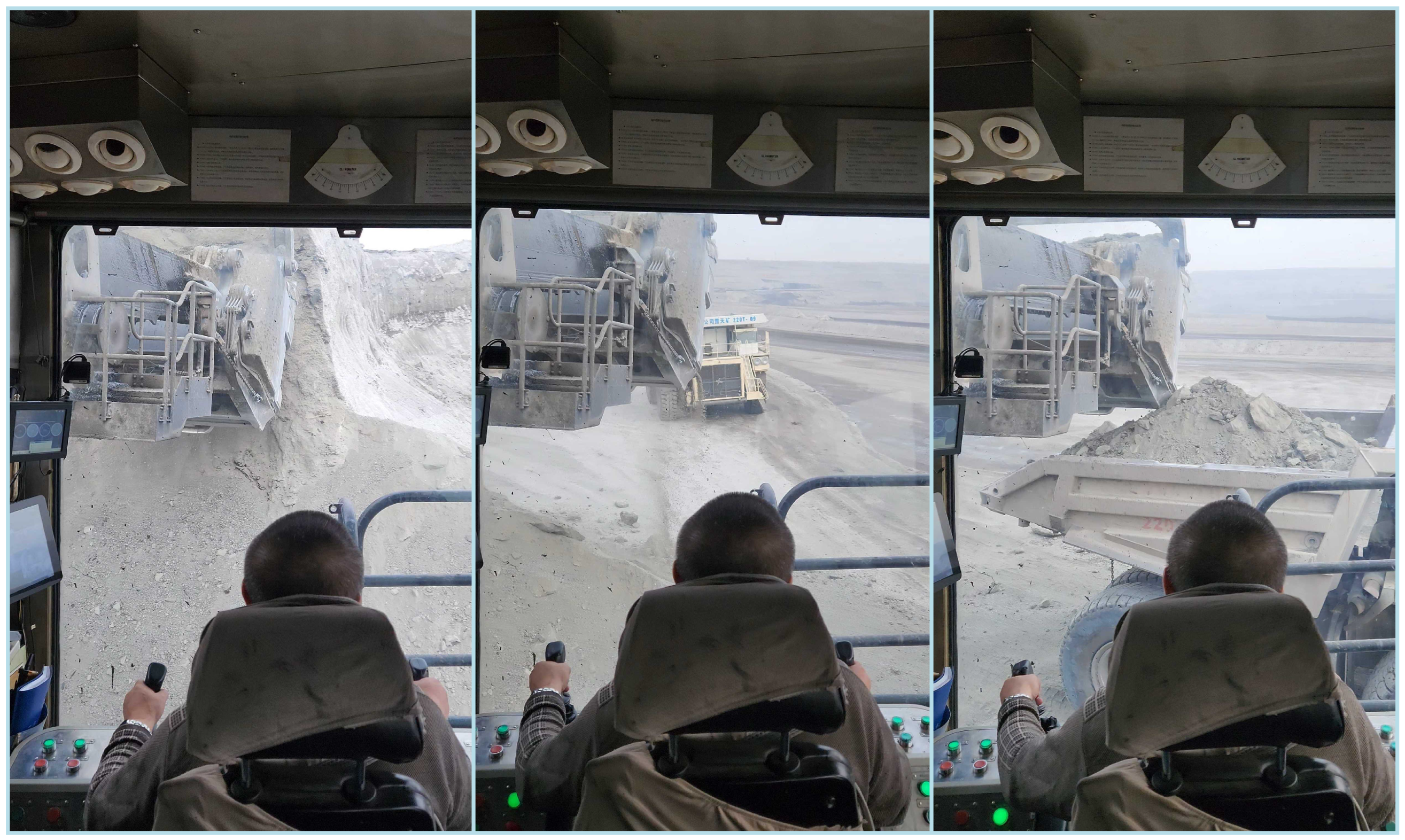
This paper specifically addresses this gap by focusing on the planning and control of the rotation and unloading phases within an excavation cycle, which directly affect operational efficiency, as the loading phase typically accounts for approximately 30–40% of the total operation time. The effectiveness of loading material into mining trucks significantly depends on precise coordination between the ERS and the truck. The swing unloading process poses a greater challenge for the operator in the electric shovel’s cabin, as shown in Figure 2, as the limited field of view makes it difficult to observe the relative position to the mining truck.

To achieve precise excavation and dumping, the relative positioning of the shovel and mining truck is first determined using LiDAR-based sensing [25]. Subsequently, trajectory planning algorithms are applied to generate an optimized unloading path, followed by the implementation of sliding-mode control, which is widely adopted in electrical, mechanical [26], and hydraulic systems [27,28] to improve precision and response speed, with RBF networks [29,30] to ensure smooth and accurate execution. By integrating trajectory planning with advanced control strategies, this research contributes to the development of intelligent mining excavation systems, paving the way for fully autonomous shovel operations.

This research focuses on utilizing LiDAR-based relative positioning and trajectory planning to improve the automation of the unloading process.

1.

Relative Positioning Accuracy: A single-line LiDAR and a dynamic DBSCAN clustering algorithm are employed to detect and identify the nearest mining truck, followed by RANSAC-based line fitting to refine truck alignment estimation.

2.

Motion Planning Complexity: A time-optimal polynomial trajectory planning approach is designed, considering mechanical constraints such as maximum acceleration and velocity, while incorporating collision avoidance strategies to prevent bucket–truck interference.

3.

Control System Precision: An RBF-enhanced sliding-mode controller (RBF-SMC) is developed to enhance trajectory tracking accuracy. The controller leverages offline-trained RBF networks for disturbance compensation, ensuring robust performance under external disturbances.

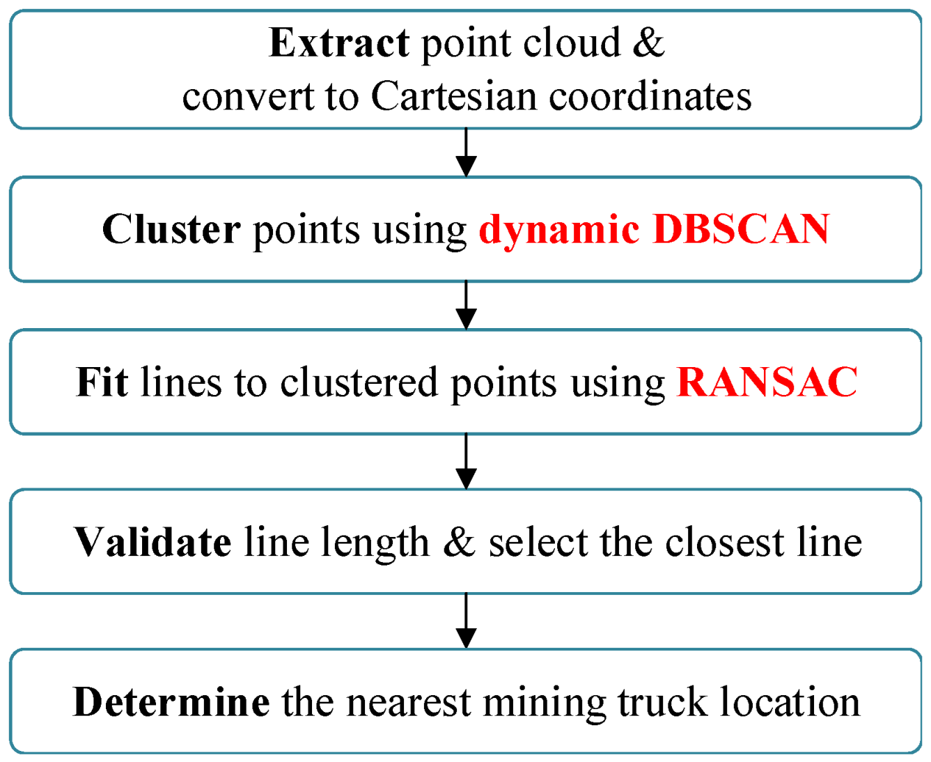
Figure 3 illustrates the complete system workflow. Starting from LiDAR-based target detection, the system extracts relative positioning information, which is subsequently used for time-optimal trajectory planning. The resulting reference trajectory is fed into the RBF-enhanced SMC, which drives the ERS motors to complete unloading. This closed-loop framework enables real-time perception–planning–control integration.

2. Model of ERS

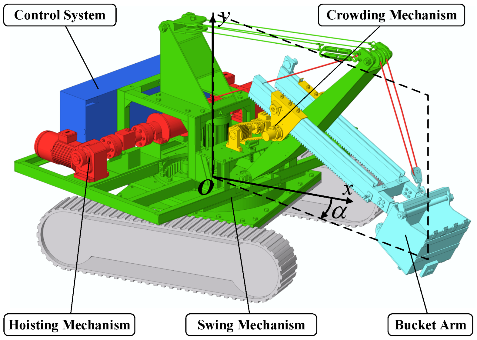
To study the motion planning and control of an ERS, it is essential to first establish its motion model. In this section, a kinematic model of the ERS is developed, analyzing the relationship between the position of the center point of the bucket and the motions of the swing mechanism and the digging mechanism.

To facilitate subsequent research on the control of the electric rope shovel, we developed a simplified scaled-down experimental prototype. Figure 4 presents the 3D model of the prototype, illustrating its geometric characteristics. As shown in Figure 4, the model of the electric rope shovel is presented using a coordinate system $O-xy\alpha (x,y,\alpha )$, where $O-xy$ represents the plane in which the ERS’s digging mechanism operates. The x-axis is aligned with the forward digging direction of the ERS in the $O-xy$ plane. The y-axis is perpendicular to the x-axis and represents the vertical direction within the digging plane. Together, $O-xy$ defines the operational plane of the digging mechanism.

The coordinate $\alpha$ represents a rotation about the y-axis. Specifically, a point in the coordinate system $(x,y,\alpha )$ is defined as the position obtained by rotating a point $(x,y)$ in the $O-xy$ plane clockwise around the y-axis by an angle $\alpha$.

In this system, the position of the bucket bottom center point P is described as $(x_p,y_p,{\alpha }_p)$, where $x_p$ and $y_p$ denote the planar position of P in the $O-xy$ plane, and ${\alpha }_p$ specifies the rotation of P out of the $O-xy$ plane, representing the angular displacement caused by the ERS swing mechanism. This hybrid system provides a concise way to describe the spatial relationship between the ERS swing mechanism and the bucket position, facilitating motion planning and control. To control the motion of the bucket of the ERS, two parameters are defined.

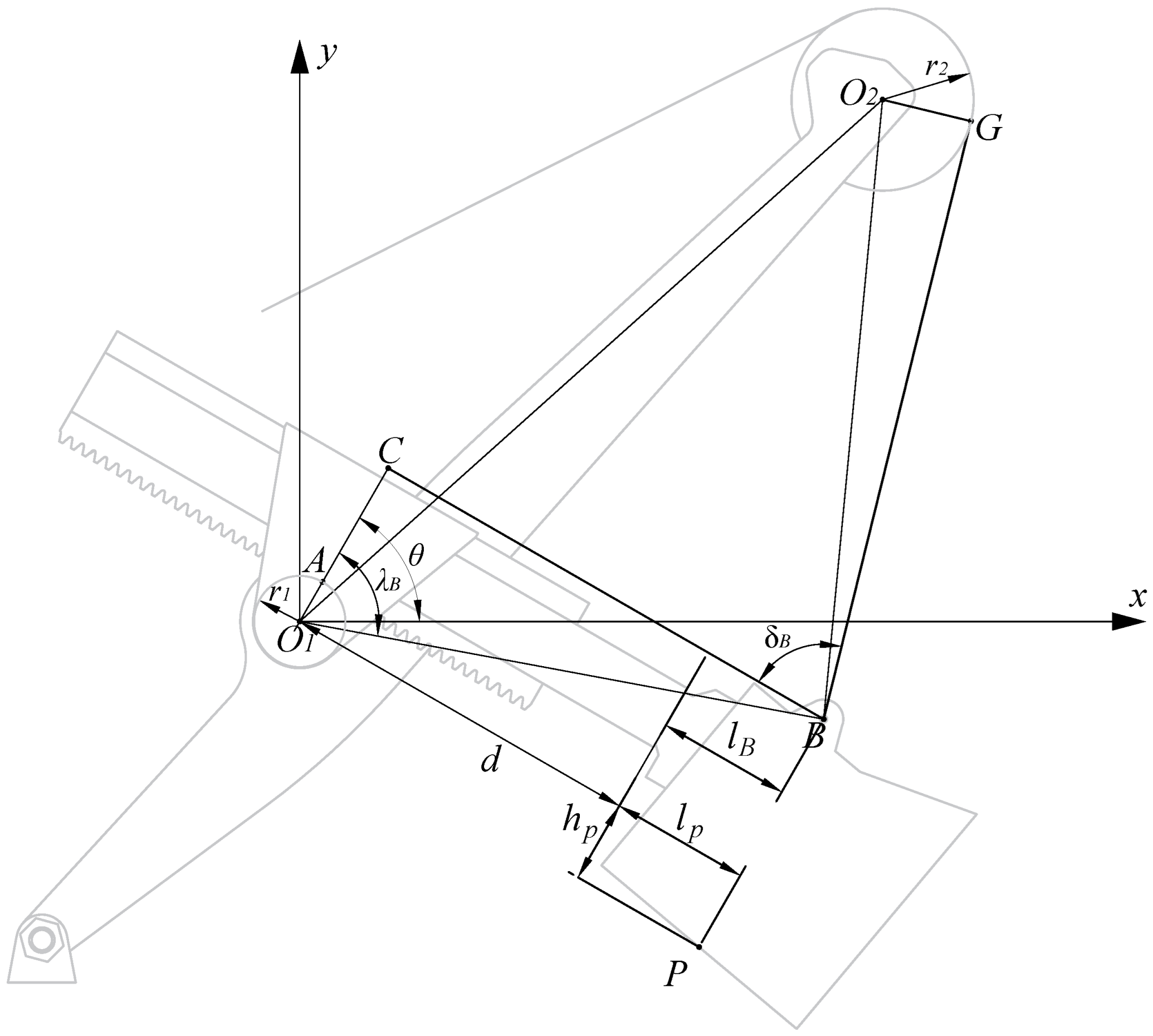
• $\theta$: the angle between the dipper handle (bucket arm) and the vertical plane.
• d: the extension length of the dipper handle relative to its pivot point at the crowd center.

Using these parameters and the other geometric dimensions as shown in Figure 5, A is the contact point between the push gear and the bucket arm, B is the hoisting point, and $B=\left(l_{O_{1}C}cos\theta +\left(d+l_B\right)sin\theta ,l_{O_{1}C}sin\theta -\left(d+l_B\right)cos\theta \right)$.

$$\overrightarrow{O_{1}P}=\left(\left(d+l_p\right)sin\theta -h_{p}cos\theta ,-\left(d+l_p\right)cos\theta -h_{p}sin\theta \right)$$

(1)

The coordinates of point P can be expressed in the hybrid coordinate system as follows:

$$\left\{\begin{array}{cc}\hfill x_p& =l_0+l_1+\left(d+l_p\right)sin\theta -h_{p}cos\theta \hfill \\ \hfill y_p& =h_1-\left(d+l_p\right)cos\theta -h_{p}sin\theta \hfill \\ \hfill {\alpha }_p& =\alpha \hfill \end{array}\right.$$

(2)

3. LiDAR-Based Relative Positioning of ERS

A critical challenge in automating the electric rope shovel (ERS) swing and truck loading process is achieving precise relative positioning between the ERS and the mining truck. The harsh environmental conditions of open-pit mining, including high dust levels and excessive water vapor in cold weather, present significant obstacles to traditional positioning systems such as vision-based systems or ultrasonic sensors. Civilian satellite positioning technology, such as GPS, typically provides an accuracy of 5 to 10 m [31,32] under open-sky conditions without ground-based augmentation systems, which is insufficient to meet the high precision required for this task. Thus, this section proposes a lower-cost and more convenient positioning method.

The consistent and well-defined geometric structure of mining trucks offers an opportunity to simplify the localization task. In actual mining operations, trucks typically travel along the excavation face and park in a position that is approximately parallel to the ERS, as illustrated in Figure 6. Given the truck’s known and fixed dimensions, the accurate identification of a few characteristic points, such as corners or side edges, can enable precise estimation of the truck’s pose relative to the ERS. This geometric insight motivates the adoption of single-line LiDAR technology, which directly leverages the truck’s structure for localization.

Since the mining truck remains stationary during the loading process performed by the ERS, a single localization measurement is sufficient to determine the relative position between the two systems for the entire operation cycle.

Furthermore, operational practices in open-pit mining ensure that both the ERS and mining trucks operate on the same horizontal plane and at a fixed height. These constraints allow the transformation of the 3D positioning problem into a 2D problem, significantly reducing the complexity of the solution while maintaining the necessary level of precision. The progress is shown in Figure 7.

3.1. Data Acquisition and Preprocessing

The laser radar is arranged within the height range of the mining truck bucket. The height of the mining truck bucket from the ground is $H_{mt}$. LiDAR data is initially recorded in polar coordinates, where each point is represented by its angle ${\theta }_L$ and distance $r_L$. To facilitate analysis, these points are converted into Cartesian coordinates.

$$x=r_L·cos{\theta }_L, y=r_L·sin{\theta }_L$$

(3)

The transformed data points $(x,y)$ represent the point cloud in the 2D plane.

3.2. Clustering and Noise Removal

The point cloud data may contain noise or isolated points. The DBSCAN (Density-Based Spatial Clustering of Applications with Noise) algorithm is regularly used to cluster points and filter out noise. The DBSCAN algorithm works as follows:

• For each point p, compute its neighborhood $N_{\epsilon }\left(p\right)$, which consists of all points within a radius $\epsilon$ of p.
• If the number of points in $N_{\epsilon }\left(p\right)$ is greater than or equal to a predefined threshold (min Pts), then p is a core point.
• Cluster core points and their neighborhoods and label points not in any cluster as noise.

The mathematical definition of the neighborhood is

$$N_{\epsilon }\left(p\right)=\left\{q\left|dist\right(p,q)\le \epsilon \right\}$$

(4)

where $\epsilon$ is the radius of the neighborhood for clustering, $minPts$ is the minimum number of points required to form a cluster, and $dist(p,q)$ is the is the Euclidean distance from point p to q.

However, the point cloud distribution is uneven, and the radius of the neighborhood for clustering in the original DBSCAN is fixed and cannot adapt to changes in point cloud density. In typical LiDAR systems, the beam scans at fixed angular intervals. Consequently, the spacing between adjacent points increases linearly with distance from the sensor, resulting in a sparser point distribution in distant regions. This leads to the non-uniform point cloud distribution commonly observed in mining environments. The clustering effect may be overly sensitive to the parameters $\epsilon$ and $minPts$. The improved method is to introduce a dynamic neighborhood radius $\epsilon \left(p\right)$, which is dynamically adjusted according to the distance from the point to the origin.

$$\epsilon \left(p\right)={\epsilon }_0+k·dist(p,O)$$

(5)

where ${\epsilon }_0$ is the base radius, used for points near the origin; k is the growth factor for points far from the origin; and $dist(p,O)$ is the Euclidean distance from point p to O.

For each point p, the neighborhood becomes

$$N_{\epsilon \left(p\right)}\left(p\right)=\left\{q\left|dist\right(p,q)\le \epsilon (p)\right\}$$

(6)

The density is defined as

$$Density\left(p\right)=\left|N_{\epsilon \left(p\right)}\left(p\right)\right|$$

(7)

A point p is considered a core point if $Density\left(p\right)\ge minPts$.

The dynamic DBSCAN iteratively calculates the adaptive radius for each point and adjusts the clustering accordingly. This approach adapts the clustering behavior to the local density of the point cloud, effectively handling variations in density.

3.3. Line Fitting and Length Validation

For the working conditions studied in this paper, the mining truck that needs to be located appears as a straight line of fixed length in the single-line radar, so it is only necessary to fit the straight line of the radar point cloud and find the one with the same length. Several alternative line-fitting algorithms were considered. RANSAC (Random Sample Consensus) was ultimately selected due to the following reasons:

• Simplicity and Efficiency: RANSAC employs a hypothesis generation and verification mechanism with low implementation complexity. Unlike learning-based methods [33,34], RANSAC does not require large-scale annotated training data, making it more transferable across different environments. Compared to conventional ICP-based registration algorithms [35], RANSAC is less prone to local minima and has been widely implemented and optimized in popular open-source libraries such as OpenCV and PCL [36].
• Superior Performance: Recent studies [37] demonstrated that RANSAC outperforms several end-to-end learning-based methods, including DGR and 3DRegNet, in terms of robustness and generalization, particularly under noisy or partially structured data.

Therefore, the RANSAC algorithm can meet the requirements. For each cluster identified by dymanic DBSCAN, a line is fitted using RANSAC. It is robust to outliers and works as follows:

Randomly sample two points from the cluster and fit the following line:

$$y=ax+b$$

(8)

Compute the perpendicular distance of all points in the cluster to the line:

$$d={\displaystyle \frac{\left|a{x}_i-y_i+b\right|}{\sqrt{a^2+1}}}$$

(9)

Identify inliers where d is less than a predefined threshold. Repeat the above steps to maximize the number of inliers and determine the best-fitting line. The inliers identified by RANSAC form a line segment. The following steps validate whether the segment’s length is approximately $L_{mt}$:

Compute the pairwise distances between all inliers:

$$dist(p_i,p_j)=\sqrt{{\left(x_i-x_j\right)}^2+{\left(y_i-y_j\right)}^2}$$

(10)

Check if any pair of points satisfies $L_{mt}-\delta \le dist(p_i,p_j)\le L_{mt}+\delta$ where $\delta$ is the length tolerance.

3.4. Finding the Closest Line and Positioning the Mining Truck

For each validated line segment, compute the minimum distance of its inliers to the origin:

$$distance=\underset{i}{min}\sqrt{x_i^2+y_i^2}$$

(11)

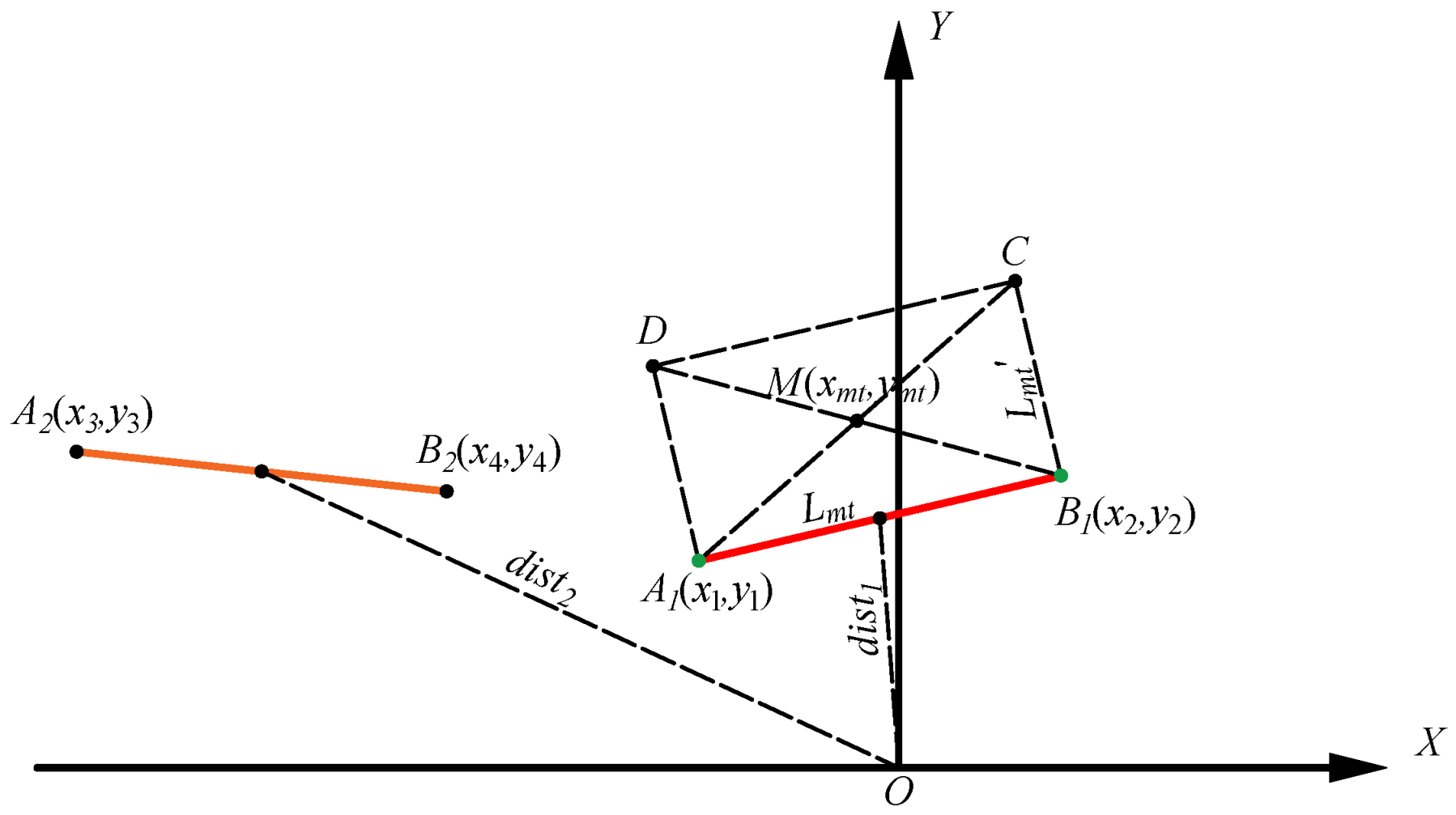
Select the line segment with the smallest distance to the origin. Record its endpoints as the start and end points of the closest line. As shown in Figure 8, $A_1{B}_1$ and $A_2{B}_2$ are the two qualified line segments identified by RANSAC, and $dis{t}_1$ and $dis{t}_2$ represent their respective distances to the origin. Based on the known geometry of the mining truck body, the positioning of the body midpoint $(x_{mt},y_{mt})$ and the ERS discharge range can be completed.

4. Unloading Trajectory Planning of ERS

Directly incorporating the time index into the trajectory optimization process will increase the complexity of iteration and even make it impossible to correctly plan the trajectory. Therefore, this paper proposes to first plan the trajectory and then compress the time axis to achieve the time-optimal trajectory. The unloading trajectory planning method proposed in this paper involves the following steps:

• Initial Calculations: Using the kinematic model, the starting and ending positions are determined by calculating the bucket arm’s angle, extension length, and the swing mechanism’s angle. The restricted area for trajectory planning is then defined based on the dimensions of the mining truck and the bucket at the end point.
• Trajectory Construction: A reference time is set, and a seventh-order polynomial trajectory is constructed to satisfy the constraints at the starting and ending points.
• Optimization: An optimization function is formulated to ensure the trajectory meets the requirements for reduced speed and acceleration, minimal changes in acceleration direction, and avoidance of restricted areas. Iterative optimization is then performed to refine the trajectory.
• Time Compression: The time axis is compressed based on the maximum speed and acceleration of the planned trajectory and the mechanical limits of the ERS. This ensures the trajectory achieves the highest possible excavation efficiency allowed by the system’s mechanical performance.

The process of refining and optimizing the trajectory is shown in Figure 4.

4.1. Initial Calculations

First, the initial position, end position, and prohibited area are calculated based on the constructed kinematic model.

The initial position ${\theta }_0$, $d_0$ and ${\alpha }_0$ can be obtained by tilt sensors, displacement transducers and angle encoders installed on the ERS.

Based on the center point of the mining truck bucket located by the LiDAR and the known bucket height $H_{mt}$, the coordinates of $MT$ are converted into the $O-xy\alpha$ coordinate system $(x_{mt},y_{mt},{\alpha }_{mt})=(\sqrt{x_L^2+y_L^2},H_{mt},arctan{\displaystyle \frac{x_L}{y_L}})$. Then, we can obtain the end position of $\theta$, d and $\alpha$ as

$$\left\{\begin{array}{c}{\theta }_f=arctan\left({\displaystyle \frac{h_1-y_{mt}}{l_1-x_{mt}}}\right)-arctan\left({\displaystyle \frac{\sqrt{{\left(x_{mt}-l_1\right)}^2+{\left(y_{mt}-h_1\right)}^2-h_p^2}}{h_p}}\right)\hfill \\ d_f=\sqrt{{\left(x_{mt}-l_1\right)}^2+{\left(y_{mt}-h_1\right)}^2-h_p^2}-l_p\hfill \\ {\alpha }_f={\alpha }_{mt}\hfill \end{array}\right.$$

(12)

Although the height of the bucket is generally higher than the truck bucket at the end of excavation and during unloading, in order to avoid collision, the movement area of the bucket should also be restricted based on the position of the mining truck during trajectory planning. Moreover, to account for the vertical clearance required between the shovel bucket and the mining truck’s dump body during unloading, which allows the bucket’s bottom plate to open, we simplify the calculations by directly setting $l_{sf}$ as the minimum allowable distance between point P and point $MT$. This constraint is used to limit the shovel bucket’s operational region, which means

$$dist(P,MT)\ge l_{sf}$$

(13)

4.2. Trajectory Construction

A conservative initial value T is set for time planning of the excavation trajectory. To ensure the smoothness of the trajectory, a seventh-order polynomial is chosen for trajectory generation. Seventh-order polynomials provide smoother jerk profiles and finer curvature control than fifth-order ones, which is crucial for heavy equipment with mechanical constraints. Construct the following position–time curve of $\alpha$, $\theta$, and d:

$$\theta \left(t\right)=\sum _{i=0}^7{a}_{\left(\theta \right)i}{({\displaystyle \frac{t}{T}})}^i,d\left(t\right)=\sum _{i=0}^7{a}_{\left(d\right)i}({{\displaystyle \frac{t}{T}})}^i,\alpha \left(t\right)=\sum _{i=0}^7{a}_{\left(\alpha \right)i}{({\displaystyle \frac{t}{T}})}^i$$

(14)

Based on the initial and final positions calculated in Step A, the start and end positions of the trajectory are defined as follows. And it is required that the velocity and acceleration at both the start and end points are zero.

$$\begin{array}{cc}\hfill & \theta \left(0\right)={\theta }_0,d\left(0\right)=d_0,\alpha \left(0\right)={\alpha }_0\hfill \\ \hfill & \theta \left(T\right)={\theta }_f,d\left(T\right)=d_f,\alpha \left(T\right)={\alpha }_f\hfill \\ \hfill & \dot{\theta }\left(0\right)=\dot{d}\left(0\right)=\dot{\alpha }\left(0\right)=0,\dot{\theta }\left(T\right)=\dot{d}\left(T\right)=\dot{\alpha }\left(T\right)=0\hfill \end{array}$$

(15)

4.3. Optimization

To achieve smooth, efficient, and obstacle-aware trajectory generation, we design a composite penalty function with different weighting coefficients to emphasize specific optimization characteristics. The total cost function is expressed as

$$J_s=c_{ve}·J_{velocity}+c_{ac}·J_{acceleration}+c_{ch}·J_{change}+c_{av}·J_{avoidance}$$

(16)

where $c_{ve}$, $c_{ac}$, $c_{ch}$, and $c_{av}$ are the weighting coefficients corresponding to the velocity, acceleration, change, and obstacle avoidance terms, respectively. These parameters allow flexible adjustment of optimization priorities under different motion scenarios.

To reduce motion intensity and enable maximal time compression (Section 4.4), the terms $J_{velocity}$ and $J_{acceleration}$ are introduced to penalize peak values of the trajectory’s first and second derivatives:

$$J_{velocity}=k_{ve1}·\underset{t}{max}\left|\dot{\theta }\left(t\right)\right|+k_{ve2}\underset{t}{·max}\left|\dot{d}\left(t\right)\right|+k_{ve3}\underset{t}{·max}\left|\dot{\alpha }\left(t\right)\right|$$

(17)

$$J_{acceleration}=k_{ac1}·\underset{t}{max}\left|\ddot{\theta }\left(t\right)\right|+k_{ac2}\underset{t}{·max}\left|\ddot{d}\left(t\right)\right|+k_{ac3}\underset{t}{·max}\left|\ddot{\alpha }\left(t\right)\right|$$

(18)

where $k_{ve\left(i\right)}$ and $k_{ac\left(i\right)}$ denote the relative importance weights assigned to each motion dimension $\theta$, d, and $\alpha$, enabling fine-grained control over the influence of each axis on the final trajectory profile.

In order to improve energy efficiency and avoid frequent jerking motions, we introduce a smoothness term $J_{change}$, which penalizes large derivatives of acceleration. Instead of using a discontinuous sign function ($sgn(·)$), a hyperbolic tangent function is applied to provide a differentiable and saturating behavior.

$$\begin{array}{cc}\hfill J_{change}=& {\int }_0^T{\left(k_{ch1}\ddot{\theta }\left(t\right){\displaystyle \frac{d}{dt}}tanh\left(k_{ch1}\ddot{\theta }\left(t\right)\right)\right)}^{2}dt+{\int }_0^T{\left(k_{ch2}\ddot{d}\left(t\right){\displaystyle \frac{d}{dt}}tanh\left(k_{ch2}\ddot{d}\left(t\right)\right)\right)}^{2}dt\hfill \\ & +{\int }_0^T{\left(k_{ch3}\ddot{\alpha }\left(t\right){\displaystyle \frac{d}{dt}}tanh\left(k_{ch3}\ddot{\alpha }\left(t\right)\right)\right)}^{2}dt\hfill \end{array}$$

(19)

where $k_{ch\left(i\right)}$ is also the weight coefficient. The tanh function is selected due to its smooth and saturating behavior, which enables stable optimization and avoids abrupt cost increases [38].

To ensure obstacle avoidance during trajectory execution, we introduce the cost term $J_{avoidance}$, which penalizes the proximity of the trajectory to restricted areas such as the mining truck body.

The penalty function is defined as:

$$\varphi \left(P\left(t\right)\right)=tanh\left(k_{av}\left(l_{sf}-dist\left(P\left(t\right),MT\right)\right)\right)+1$$

(20)

where $P\left(t\right)$ denotes the current trajectory point, $dist\left(P\right(t),MT)$ represents the Euclidean distance from the trajectory to the mining truck $MT$, and $l_{sf}$ is a predefined safety distance. The coefficient $k_{av}$ controls the steepness of the penalty increase as the trajectory approaches the restricted boundary.

The total obstacle avoidance cost is then computed as

$$J_{avoidance}={\int }_0^T\varphi \left(P\left(t\right)\right)dt$$

(21)

This formulation encourages the trajectory to remain outside the restricted zone defined by $l_{sf}$ while maintaining optimization stability and numerical smoothness.

The trajectory optimization process utilizes the Sequential Least Squares Programming (SLSQP) algorithm, a practical implementation of the Sequential Quadratic Programming (SQP) framework, to iteratively refine the trajectory while satisfying the given constraints. SLSQP is particularly well suited for problems with nonlinear objectives and constraints, as it combines the efficiency of quadratic programming with the flexibility required to handle nonlinearity. This makes it ideal for complex trajectory planning scenarios involving multiple competing objectives, such as minimizing velocity, acceleration, and trajectory deviation while simultaneously avoiding restricted areas. This step allows for efficient convergence to a locally optimal solution that adheres to all physical and operational constraints. To initialize the optimization, all polynomial coefficients are sampled from a small uniform distribution within the range $[0,0.1]$. This random but smooth initialization ensures numerical stability and avoids severe oscillations in the initial trajectory while allowing sufficient flexibility for the optimizer to explore the solution space.

Regarding second-order information, the SLSQP implementation employed in this study does not require an explicit Hessian matrix. Instead, it approximates the Hessian of the Lagrangian using a quasi-Newton BFGS update scheme, with gradients estimated via finite-difference methods. This automatic approximation balances computational efficiency with solution accuracy and is well suited to the dimensionality and structure of the trajectory planning problem.

4.4. Time Compression

Once the optimal trajectory is obtained, time compression is applied to achieve time-optimal performance while respecting mechanical limits. A compression factor ${\beta }_t$ is computed based on the ratio ${\beta }_v$(${\beta }_t$) of the maximum trajectory velocity (acceleration) to the system’s allowable maximum velocity (acceleration).

$$\begin{array}{cc}\hfill & {\beta }_t=max({\beta }_v,{\beta }_a)\hfill \\ \hfill & {\beta }_v=max({\displaystyle \frac{\underset{t}{max}\left|\dot{\theta }\left(t\right)\right|}{{\omega }_{max-\theta }}},{\displaystyle \frac{\underset{t}{max}\left|\dot{d}\left(t\right)\right|}{v_{max-d}}},{\displaystyle \frac{\underset{t}{max}\left|\dot{\alpha }\left(t\right)\right|}{{\omega }_{max-\alpha }}})\hfill \\ \hfill & {\beta }_a=max({\displaystyle \frac{\underset{t}{max}\left|\ddot{\theta }\left(t\right)\right|}{a_{max-\theta }}},{\displaystyle \frac{\underset{t}{max}\left|\ddot{d}\left(t\right)\right|}{a_{max-d}}},{\displaystyle \frac{\underset{t}{max}\left|\ddot{\alpha }\left(t\right)\right|}{a_{max-\alpha }}})\hfill \end{array}$$

(22)

which ensures that the time axis is compressed without exceeding system limitations. Finally, the trajectory time is scaled by $T^{\prime }={\beta }_{t}T$, effectively reducing the total time while maintaining the trajectory’s shape and satisfying velocity and acceleration constraints.

This approach guarantees compliance with spatial constraints while minimizing execution time within the bounds of the system’s mechanical limitations, thereby enhancing operational efficiency. Although the time compression strategy does not attain strict global time optimality, it constitutes a practically near-optimal solution that balances computational tractability with implementation feasibility, making it well suited for real-world engineering deployment.

5. RBF-Enhanced Sliding-Mode Control of ERS

In this section, an RBF-enhanced sliding-mode controller (RBF-SMC) is proposed. The structure of RBF-SMC is shown as Figure 9. Compared to MPC and adaptive control, the proposed RBF-SMC offers a better tradeoff between real-time feasibility and robustness under uncertain disturbances.

The ERS is driven by three motors with similar structures. Consider the following motor drive model:

$$J·\ddot{\theta }=u-F_{friction}+F_{disturbance}$$

(23)

where $\theta$ is the rotation angle of the motor, J is the rotational inertia, u is the control input, $F_{friction}$ is the frictional resistance applied to the motor, and $F_{disturbance}\le D$ is the unknown external interference and load changes. Considering that the ERS has a known physical structure and the mass of the excavated material is relatively small compared to the ERS, J can be regarded as a known constant. Rewrite (23) into the form of state equation

$$\ddot{x}={\displaystyle \frac{1}{J}}·u+f\left(x\right)$$

(24)

where x is the state of system, and $f\left(x\right)=-{\displaystyle \frac{1}{J}}\left(F_{friction}+F_{disturbance}\right)$. Define the sliding-mode surface as

$$s=\dot{e}+ce,\left(c>0\right)$$

(25)

where e is the error, $e=x_d-x$.

Therefore, a range-constrained regularized RBF network (RCRRBF) is used to approximate them. Its general output form is given as

$$f\left(x\right)={\mathbf{W}}^T\mathbf{h}\left(x\right)+\epsilon$$

(26)

where $\mathbf{h}={\left[h_i\right]}^T$ is the output of the Gaussian basis functions, $\mathbf{W}$ is the weight vector, and $\epsilon$ represents the approximation error, satisfying $\left|\epsilon \right|\le {\epsilon }_M$. The Gaussian basis functions are defined as

$$h_i\left(x\right)=exp\left(-{\displaystyle \frac{{∥x-c_i∥}^2}{2b_i^2}}\right)$$

(27)

where $c_i$ is the center and $b_i$ is the width of the i-th basis function. The goal is to approximate a target function while constraining the network output $f\left(x\right)$ to lie within a known range $\left[f_{min},f_{max}\right]$. Direct application of standard RBF networks may not ensure this constraint, particularly in cases where extrapolation or noise occurs.

To ensure the network output remains within the desired range while minimizing the approximation error, we define a total loss function consisting of two components: the mean squared error (MSE) loss and a range-constrained regularization term. The total loss is expressed as

$$\begin{array}{cc}\hfill & Los{s}_{total}=Los{s}_{MSE}+\lambda ·Los{s}_{Reg}\hfill \\ \hfill & Los{s}_{MSE}={\displaystyle \frac{1}{N}}\sum _{i=1}^N{\left(f\left(x_i\right)-y_i\right)}^2\hfill \\ \hfill & Los{s}_{Reg}={\displaystyle \frac{1}{N}}\left[max\left(0,f\left(x_i\right)-f_{max}\right)+max\left(0,f_{min}-f\left(x_i\right)\right)\right]\hfill \end{array}$$

(28)

where $\lambda$ is the regularization coefficient, $y_i$ is the target value, $f\left(x_i\right)$ is the network output, and N is the number of samples. This term penalizes outputs $f\left(x_i\right)$ that fall outside the range $\left[f_{min},f_{max}\right]$. The network parameters are optimized via gradient descent, incorporating the gradients of both the MSE loss and the regularization term.

To ensure the stability of the proposed range-constrained RBF network, we define a Lyapunov candidate function

$${\mathbf{V}}_W={\displaystyle \frac{1}{2}}{∥\mathbf{W}-{\mathbf{W}}^{*}∥}^2$$

(29)

where ${\mathbf{W}}^{*}$ is the optimal weight vector that minimizes $Los{s}_{total}$. The time derivative of ${\mathbf{V}}_W$ is given by

$${\dot{\mathbf{V}}}_W={\left(\mathbf{W}-{\mathbf{W}}^{*}\right)}^T{\displaystyle \frac{\partial Los{s}_{total}}{\partial \mathbf{W}}}$$

(30)

Since gradient descent ensures that the weights are updated in the direction of decreasing $Los{s}_{total}$, we have ${\dot{\mathbf{V}}}_W<0$, which guarantees that $\mathbf{W}$ converges asymptotically to ${\mathbf{W}}^{*}$.

The control output is designed as

$$u=J\left(-\hat{f}\left(x\right)+{\ddot{x}}_d+c\dot{e}+\eta \mathrm{sgn}\left(s\right)\right),(\eta \ge D)$$

(31)

Combining (25) and (31), we have

$$\begin{array}{cc}\hfill \dot{s}& =\ddot{e}+c\dot{e}={\ddot{x}}_d-f\left(x\right)-d\left(t\right)+c\dot{e}\hfill \\ \hfill & ={\ddot{x}}_d-f\left(x\right)-\left(-\hat{f}\left(x\right)+{\ddot{x}}_d+c\dot{e}+\eta \mathrm{sgn}\left(s\right)\right)-d\left(t\right)+c\dot{e}\hfill \\ \hfill & =\hat{f}\left(x\right)-f\left(x\right)-\eta \mathrm{sgn}\left(s\right)-d\left(t\right)\hfill \\ \hfill & ={\tilde{\mathbf{W}}}^T\mathbf{h}\left(x\right)-\epsilon -\eta \mathrm{sgn}\left(s\right)-d\left(t\right)\hfill \end{array}$$

(32)

where $\tilde{\mathbf{W}}={\mathbf{W}}^{*}-\hat{\mathbf{W}}$.

Even though the network has been trained to obtain an ideal initial estimate of the weights $\hat{\mathbf{W}}$, its role is only to accelerate early-stage convergence. To ensure that the controller remains effective in the presence of unmodeled dynamics and unknown disturbances, especially those beyond the scope of the training data, we design an adaptive law for the network weights as follows:

$$\dot{\hat{\mathbf{W}}}=-\gamma s\mathbf{h}\left(x\right)$$

(33)

The Lyapunov function of the controller is defined as

$$V={\displaystyle \frac{1}{2}}{s}^2+{\displaystyle \frac{1}{2\gamma }}{\tilde{\mathbf{W}}}^T\tilde{\mathbf{W}}$$

(34)

where $\gamma ={{\gamma }_{max}}^{1-e^{-\mu t}}$,$(\mu >0)$ and time derivate of V is

$$\begin{array}{cc}\hfill \dot{V}& =s\dot{s}+{\displaystyle \frac{1}{\gamma }}{\tilde{\mathbf{W}}}^T\dot{\tilde{\mathbf{W}}}\hfill \\ \hfill & ={\tilde{\mathbf{W}}}^T\left(s\mathbf{h}\left(x\right)-{\displaystyle \frac{1}{\gamma }}\dot{\hat{\mathbf{W}}}\right)+s\left(-\epsilon -\eta \mathrm{sgn}\left(s\right)-d\left(t\right)\right)\hfill \\ \hfill & =s\left(-\epsilon -\eta \mathrm{sgn}\left(s\right)-d\left(t\right)\right)=\left(-\epsilon -d\left(t\right)\right)s-\eta \left|s\right|\hfill \end{array}$$

(35)

Since the error of the RCRRBF network is close to 0, taking $\eta \ge \left|{\epsilon }_M+D\right|$ can ensure that $\dot{V}\le 0$; that is, the sliding-mode controller is convergent.

6. Experiment

In this section, we will evaluate the feasibility of the proposed positioning and trajectory planning method and the accuracy of the control method using a scaled model.

6.1. Experiment Setup

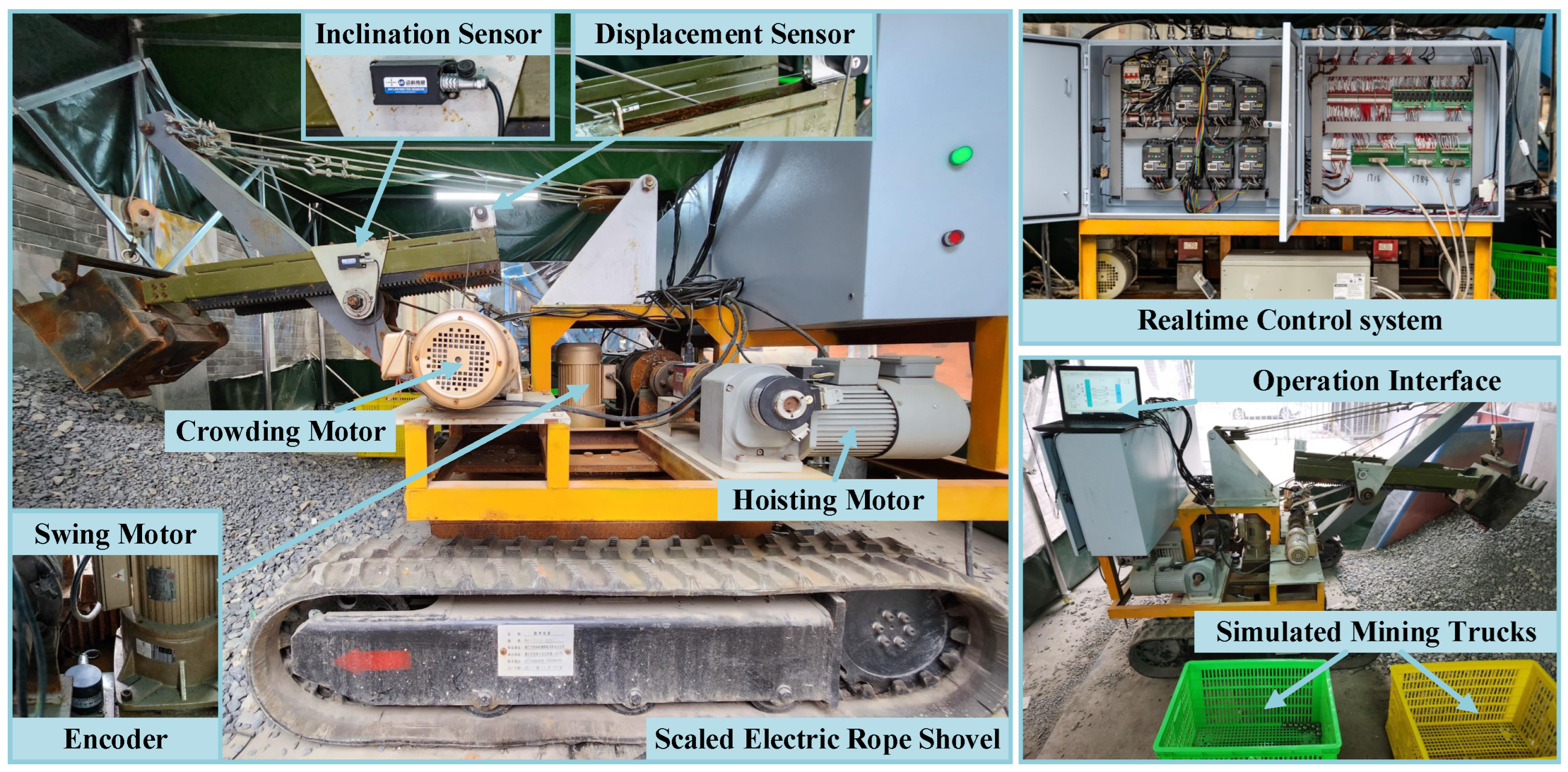
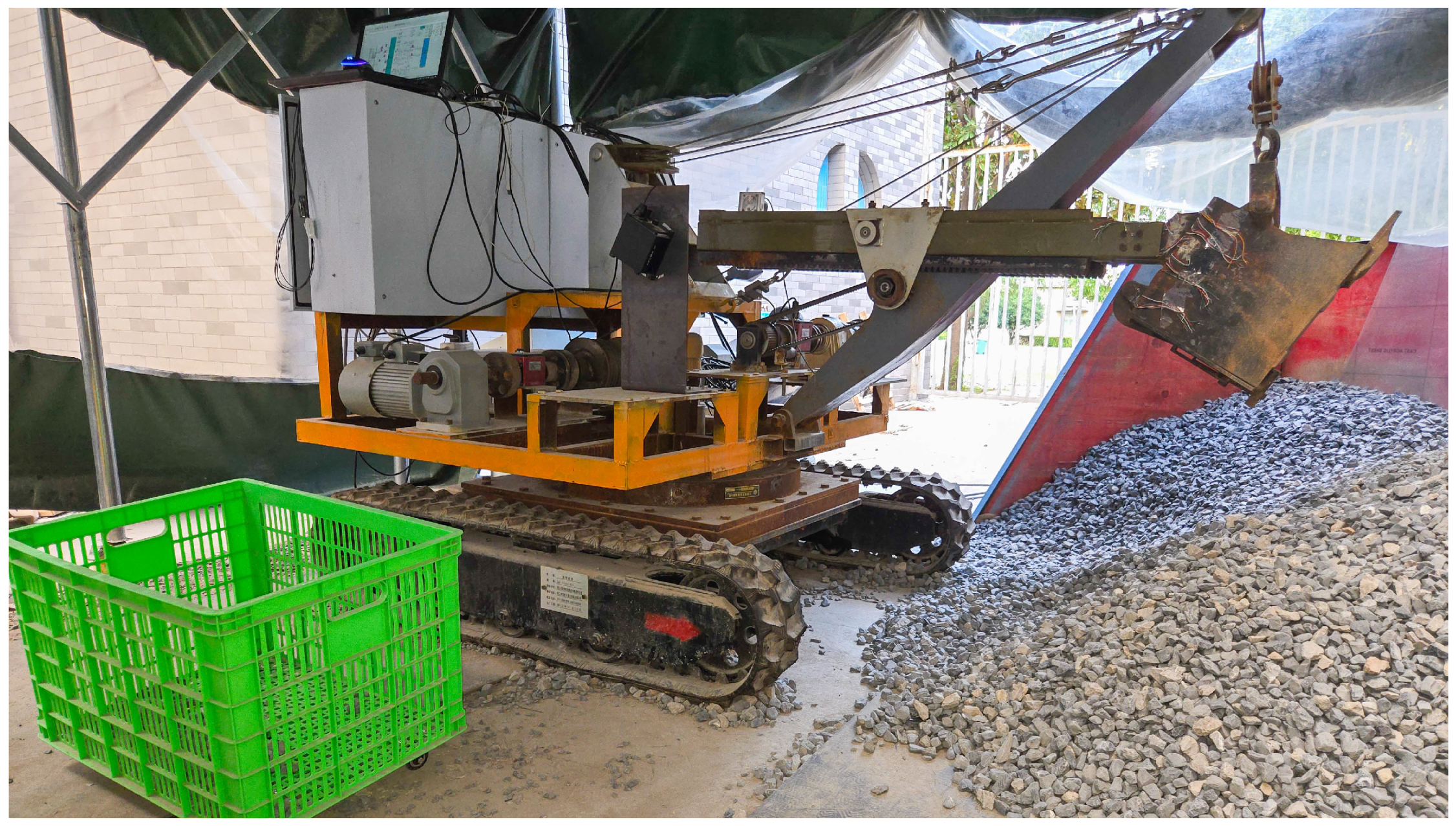
The experimental bench is presented in Figure 10, which consists of a scaled electric rope shovel, a measurement system, and a control system. The scaled model, constructed at a 1:9 scale based on the WK-10 electric rope shovel, is designed to replicate the real machine’s key functionalities, including excavation, swing, and walking operations. The measurement system includes a singe-line LiDAR, a motor encoder, a displacement sensor, and an inclination sensor to capture the shovel’s movements. The control system comprises an xPC-based real-time controller and a host computer. In this architecture, the host functions as the upper-level controller, responsible for radar data processing, target recognition, and trajectory planning. It communicates with the xPC real-time controller via TCP/IP, transmitting reference trajectories and receiving system feedback in real time. This hierarchical design enables the host to perform computationally intensive perception and planning tasks, while the xPC target ensures deterministic, low-latency execution of the control algorithm. The main technical parameters of the scaled ERS experimental bench are listed in

Table 1. Main technical parameters of the scaled ERS experimental bench.

Item	Specification
Dimensions (L*W*H)	$2800\times 1500\times 1588$ mm
Total weight	$1.5$ t
Hoisting motor power	$1.1$ kW $\ast 2$
Hoisting force	4000 N
Crowd motor power	$0.75$ kW
Crowd force	2000 N
Walking motor power	$1.5$ kW $\ast 2$
Swing motor power	$1.1$ kW
Maximum excavation radius	2030 mm
Maximum excavation height	1350 mm

. The relevant parameters are listed in

Table 2. Physical parameters of the system.

Parameter	Value	Parameter	Value
$H_{mt}$	400 mm	$L_{mt}$	675 mm
$h_1$	340 mm	$l_1$	340 mm
$l_{O_{1}C}$	210 mm	$l_B$	307 mm
$h_P$	104 mm	$l_P$	313 mm
$x_{O_2}(O_1-xy)$	1442 mm	$y_{O_2}(O_1-xy)$	1040 mm
$r_1$	50 mm	$r_2$	50 mm
$r_h$	90 mm	$N_s$	2.88
$J_c$	2.26 kg·m2	$J_h$	24.6 kg·m2
$J_s$	37.9 kg·m2	$h_0$	539 mm
$l_0$	420 mm	$h_{aviod}$	300 mm

. The models and parameters of each motor are listed in

Table 3. Models and parameters of each motor.

Name	Model	Power	Torque	Speed
Swing	NVC32-1100-60	1.1 kW	337 Nm	25 rpm
Crowd	NCH28-750-30	0.75 kW	135 Nm	50 rpm
Hoist	SZG32-H-1100-30	1.1 kW	175 Nm	50 rpm

.

6.2. Relative Positioning and Trajectory Planning

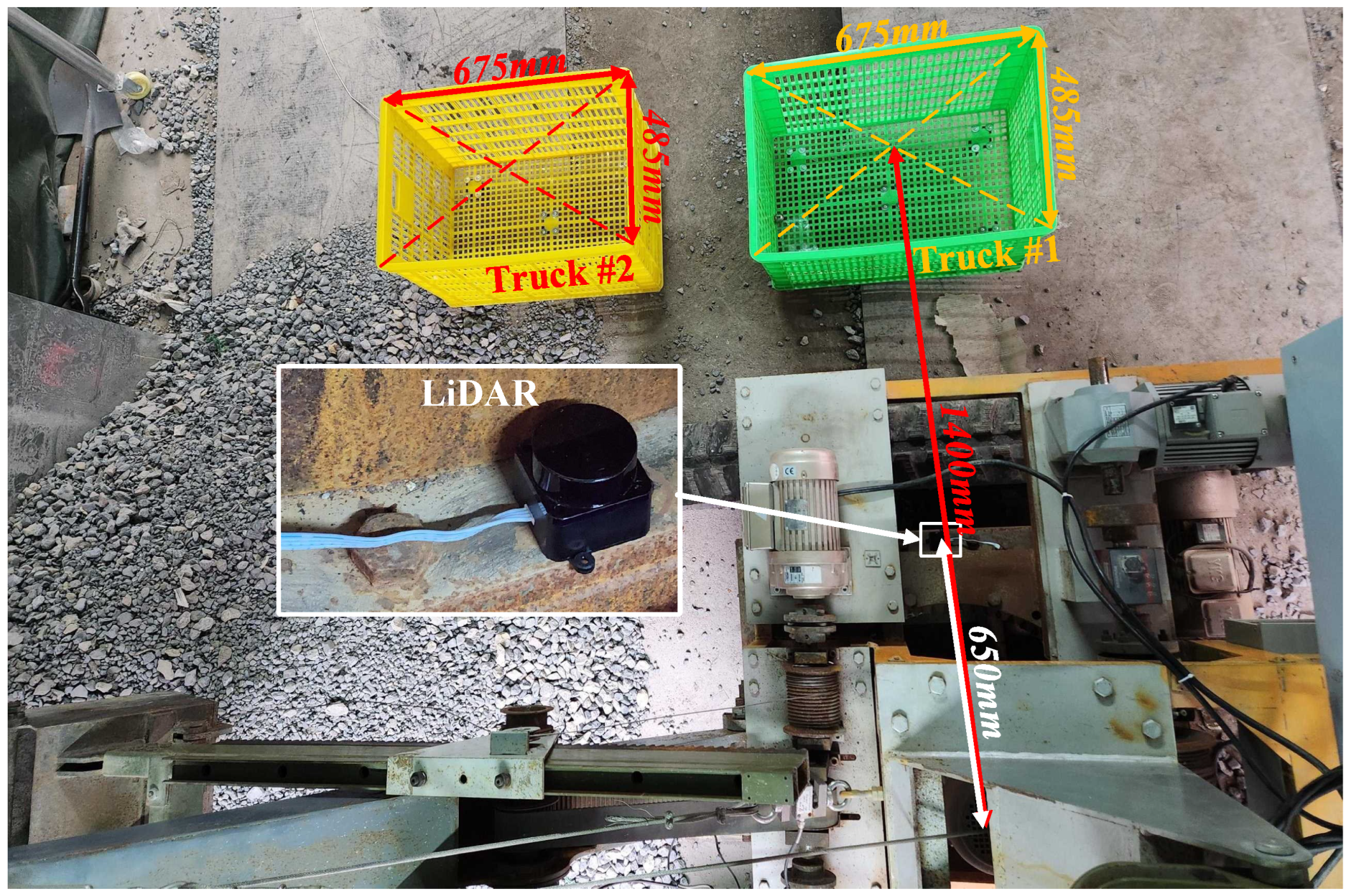
To verify the effectiveness of the relative positioning and trajectory planning methods, two cargo boxes (675 mm × 485 mm × 400 mm) are used to simulate mining trucks for positioning and planning experiments, as shown in Figure 11. The green one (Truck #1) is the truck being loaded, and the yellow one (Truck #2) is the truck waiting to be loaded. The LiDAR is placed 650mm to the right of the rotation center.

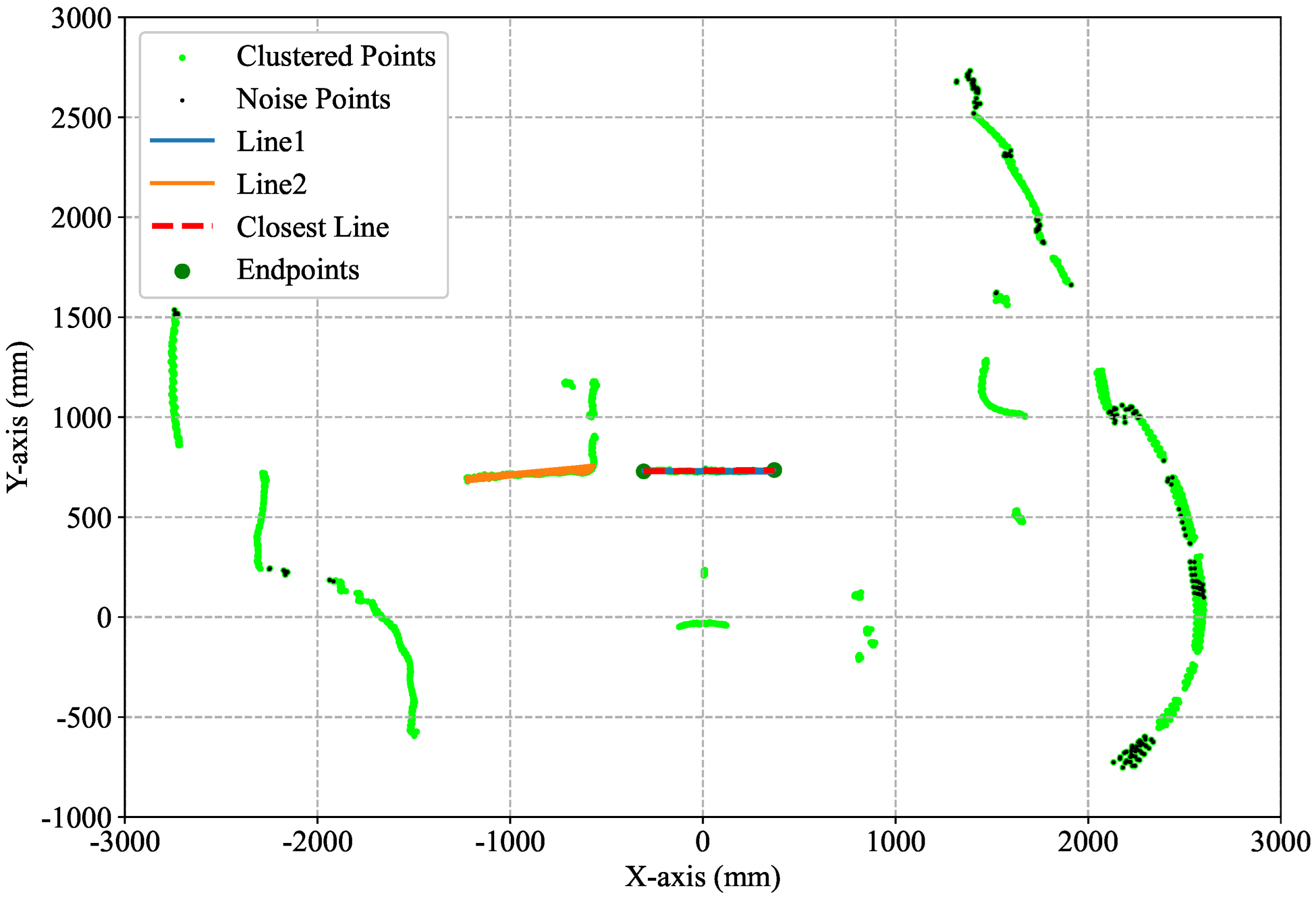
The LiDAR positioning results are shown in Figure 12. Using the dynamic DBSCAN algorithm, the points are classified into noise points (black) and valid points (green).

To determine appropriate clustering parameters, we performed a sensitivity analysis by varying ${\epsilon }_0$, k, and $minPts$ across a range of values. For each parameter combination, the proportion of points classified as noise was computed, as illustrated in Figure 13.

This analysis reveals a trade-off between removing noisy outliers and preserving sufficient valid data for reliable line detection. A small ${\epsilon }_0$ or k tends to over-segment the point cloud, while a large value may include spurious points into valid clusters. Based on the balance between noise suppression and data retention, we selected (${\epsilon }_0=20$, $k=0.01$, $minPts=10$) as the final configuration, which yields a reasonable noise ratio and ensures cluster continuity for subsequent geometric analysis.

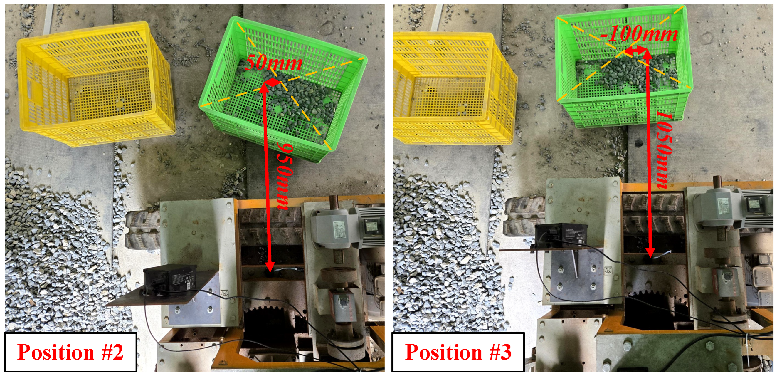
The RANSAC algorithm ($L_{mt}=675$, $\delta =15$) is then applied to fit straight-line segments and identify the nearest one to the electric shovel (highlighted in red) along with its two endpoints. The actual measured values are shown in Figure 12. We then changed the truck’s position and conducted two more positioning experiments, as shown in Figure 14. The results are shown in

Table 4. LiDAR positioning results.

Position 1: $\mathit{X}=0$ mm, $\mathit{Y}=750$ mm
Number of Tests	1	2	3	4	5
X(mm)	$20.8$	$16.3$	$2.0$	$3.0$	$-7.1$
Y(mm)	731	731	726	730	726
Error of X(mm)	$-20.8$	$-16.3$	$-2.0$	$-3.0$	$7.1$
Error of Y(mm)	19	19	24	20	24
Position 2: $X=50$ mm, $Y=950$ mm
Number of Tests	1	2	3	4	5
X(mm)	$44.0$	$54.2$	$68.4$	$35.9$	$52.7$
Y(mm)	972	923	962	968	941
Error of X(mm)	$-6.0$	$4.2$	$18.4$	$-14.1$	$2.7$
Error of Y(mm)	22	$-27$	12	18	$-9$
Position 3: $X=-100$ mm, $Y=1050$ mm
Number of Tests	1	2	3	4	5
X(mm)	$-79.2$	$-119.1$	$-106.7$	$-84.1$	$-96.3$
Y(mm)	1038	1029	1073	1027	1077
Error of X(mm)	$20.8$	$-19.1$	$-6.7$	$15.9$	$3.7$
Error of Y(mm)	$-12$	$-21$	23	$-23$	27

, with five repeated measurements conducted at each position. The reported X and Y values represent the coordinates of the geometric center of the simulated mining truck. As summarized in

Table 5. LiDAR positioning error.

	X	Y
Mean Absolute Error	10.85 mm	20.0 mm
Root Mean Square Error	13.04 mm	20.67 mm
Maximum Absolute Error	21.1 mm	27.0 mm

, the mean absolute errors (MAEs) in the X and Y directions are 10.85 mm and 20.0 mm, respectively, with corresponding root mean square errors (RMSEs) of 13.04 mm and 20.67 mm. The maximum absolute errors are 21.1 mm in X and 27.0 mm in Y.

It is important to note that the LiDAR used in the scaled experiment is a full-function sensor with fixed resolution and ranging accuracy. As such, the observed positioning errors are not subject to scaling by the physical model ratio [39,40]. In other words, the measured error values reflect the actual performance expected in full-scale deployment. Given that these errors are significantly smaller than the physical dimensions of the mining truck, the proposed method is sufficiently accurate for localization and automated truck loading tasks.

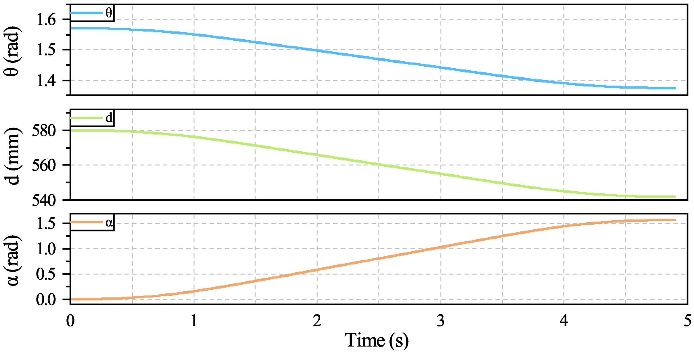
Based on the previously established excavator motion model, the calculated swing unloading point, which is the endpoint of the trajectory, is $(1.3743,542.27,1.5708)$. Consider the case where no obstacle avoidance is required (Condition 1, assumed starting point $(1.5708,580,0)$), as shown in Figure 15. Based on the obtained relative position information of the mining truck, a time-optimal trajectory is planned using the method described in Section 4, with $T=10$, $c_{ve\left(i\right)}=c_{ac\left(i\right)}=c_{ch\left(i\right)}=1$, $k_{ve\left(i\right)}=k_{ac\left(i\right)}=k_{ch\left(i\right)}=1$. The polynomial coefficient optimization process is shown in Figure 16. Since the swing motion has the largest amplitude during the unloading process, the maximum acceleration and velocity constraints of the swing determine the value of ${\beta }_t$. Considering the mechanical structure and drive capability, we set ${\omega }_{max}=0.45$ and $a_{max}=1$. When $T=10s$,$\underset{t}{max}\left|\dot{\alpha }\left(t\right)\right|=0.211$, and $\underset{t}{max}\left|\ddot{\alpha }\left(t\right)\right|=0.107$, resulting in ${\beta }_t=0.49$. Thus, the optimized trajectory time is $T^{\prime }=4.9s$, and the curves of $\theta$, d and $\alpha$ are shown in Figure 17.

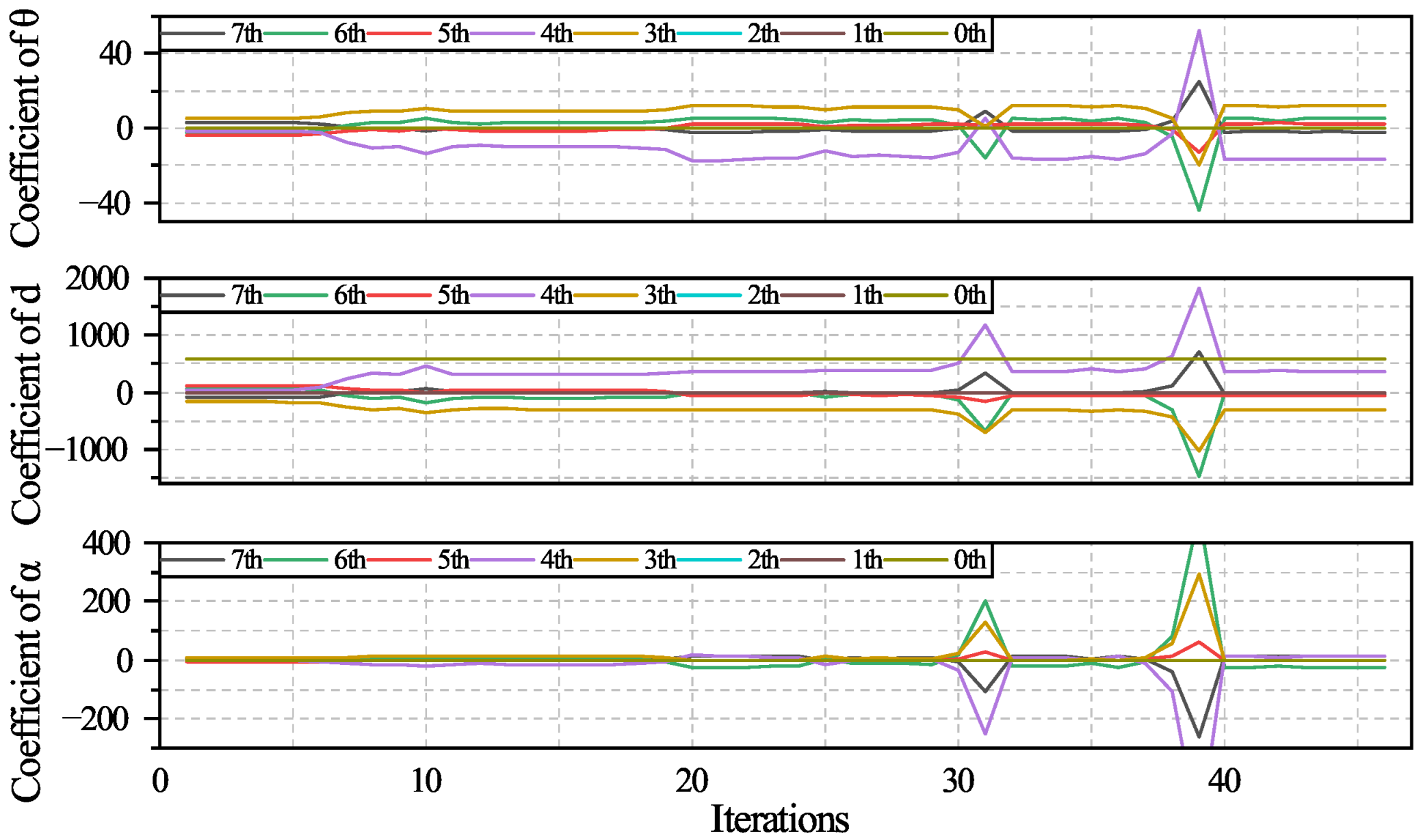
In certain operating conditions (Condition 2, starting point $(0.2010,580,0)$), as shown in Figure 18, the endpoint of the excavation trajectory is lower than the unloading point. Direct swing trajectory planning in such cases may result in a collision between the bucket and the mining truck. Therefore, obstacle avoidance is considered by setting a safety distance of $l_{sf}=200$ mm and a penalty weight of $c_{av}=10$. The choice of $l_{sf}$ takes into account the bucket dimensions and the structural clearance required for the bottom gate mechanism of the prototype, ensuring that sufficient clearance is maintained to prevent collisions during the autonomous swing operation. The coefficient optimization process and the final trajectory are shown in Figure 19 and Figure 20 with $T=6.3$ s. To avoid obstacles, the trajectory planner generates a motion path that maintains a greater distance from the obstacle points. As a result, the planned trajectory exhibits an earlier lifting action compared to the nominal curve, enabling the bucket to gain sufficient height in advance to avoid potential collisions with the mining truck during the subsequent swing.

To evaluate the computational performance of the full autonomous operation pipeline, we measured the time consumption of three key steps: LiDAR scanning, DBSCAN+RANSAC-based truck localization, and SLSQP-based trajectory planning. Each step was executed 20 times under identical conditions. The tests were conducted on a laptop with Intel i7-10750H and 16GB RAM. The time cost of each step is shown in

Table 6. Time Cost of Each Step.

	LiDAR Scanning	DBSCAN + RANSAC Localization	SLSQP Trajectory Planning
Average	1343 mm	673 mm	4481 ms
Max	1405 mm	741 mm	5521 ms
Min	1280 mm	645 mm	4363 ms

.

These results confirm that the total processing time from sensing to trajectory generation remains under 8 s, which is acceptable for real-time deployment.

Considering the operational characteristics of the ERS, the unloading point can be determined as soon as the mining truck arrives. Likewise, once the bucket begins excavating the pile surface, the starting point of the swing trajectory becomes known. Since the excavation phase typically lasts 10–20 s, there is sufficient time to complete the planning process within the same operation cycle. Therefore, the proposed planning method is suitable for enabling continuous and uninterrupted autonomous operation. Further acceleration is possible by reducing problem dimensionality or leveraging parallel hardware in future implementations.

The final coefficients of the trajectories of condition 1 and 2 are shown in

Table 7. Polynomial coefficient optimization results.

	Condition 1			Condition 2
	$\mathit{\theta }$	$\mathit{d}$	$\mathit{\alpha }$	$\mathit{\theta }$	$\mathit{d}$	$\mathit{\alpha }$
7th	−6.172	−1190	49.21	−1.830	−23.70	13.48
6th	21.60	4166	−172.2	5.195	−9.473	−23.59
5th	−28.96	−5585	230.8	2.440	−57.37	−0.6856
4th	18.39	3546	−146.6	−16.66	351.9	13.51
3th	−5.056	−975.2	40.31	12.03	−299.4	−1.144
2th	0	0	0	0	0	0
1th	0	0	0	0	0	0
0th	1.570	580	0	0.201	580	0

.

6.3. Simulation of RCRRBF Network

In real-world heavy-duty construction machinery applications, it is often difficult to directly measure shaft torque. Similarly, in the scaled-down experimental platform, the external disturbance acting on the motor cannot be directly obtained. As a result, it is not possible to obtain an accurate reference value for the disturbance in real experiments to validate the accuracy of the RCRRBF network estimation. To address this limitation, we construct a training dataset using a simulation model and, after offline training, apply the trained RCRRBF network to the actual control system.

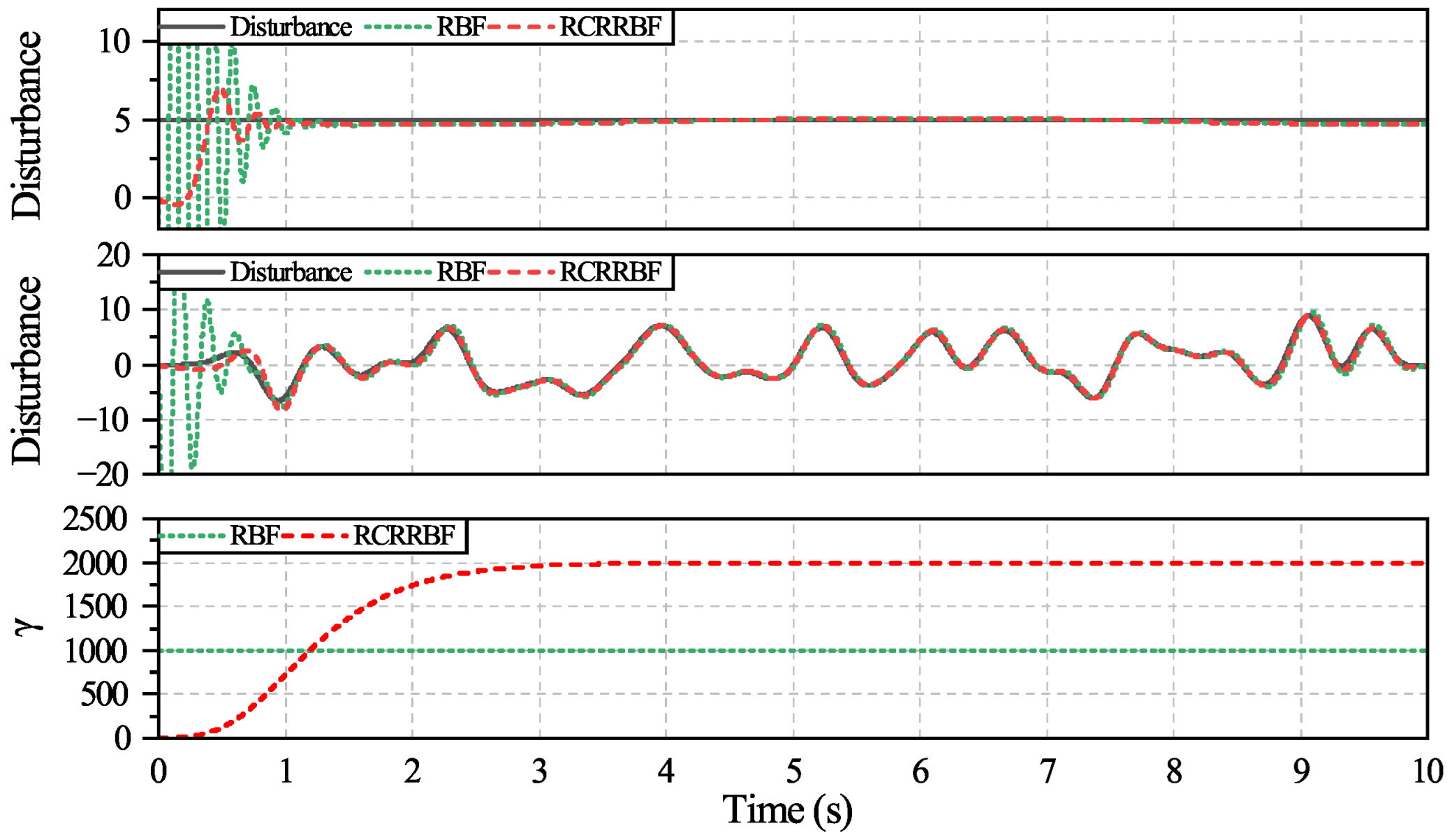
However, due to experimental constraints, the error between the RCRRBF-estimated disturbance and the actual disturbance cannot be directly compared in real experiments. Therefore, we have included a simulation experiment section in the paper to verify the RCRRBF network’s disturbance estimation capability using simulation data and to analyze its error characteristics. This simulation experiment supports the effectiveness of the RCRRBF network in real systems, compensating for the lack of a real disturbance reference in physical experiments. As shown in Figure 21, the results demonstrate that the RCRRBF network ($M=10$, $Epochs=1000$, $Lr=1$, $Lr\_decay=0.9999$) improves initial stability and maintains comparable tracking performance to the traditional RBF network under both constant and random disturbances. The gradual increase in $\gamma$ effectively reduces initial divergence, making the RCRRBF network more robust and adaptive to system variations.

6.4. Preformance Experiment of RBF-SMC

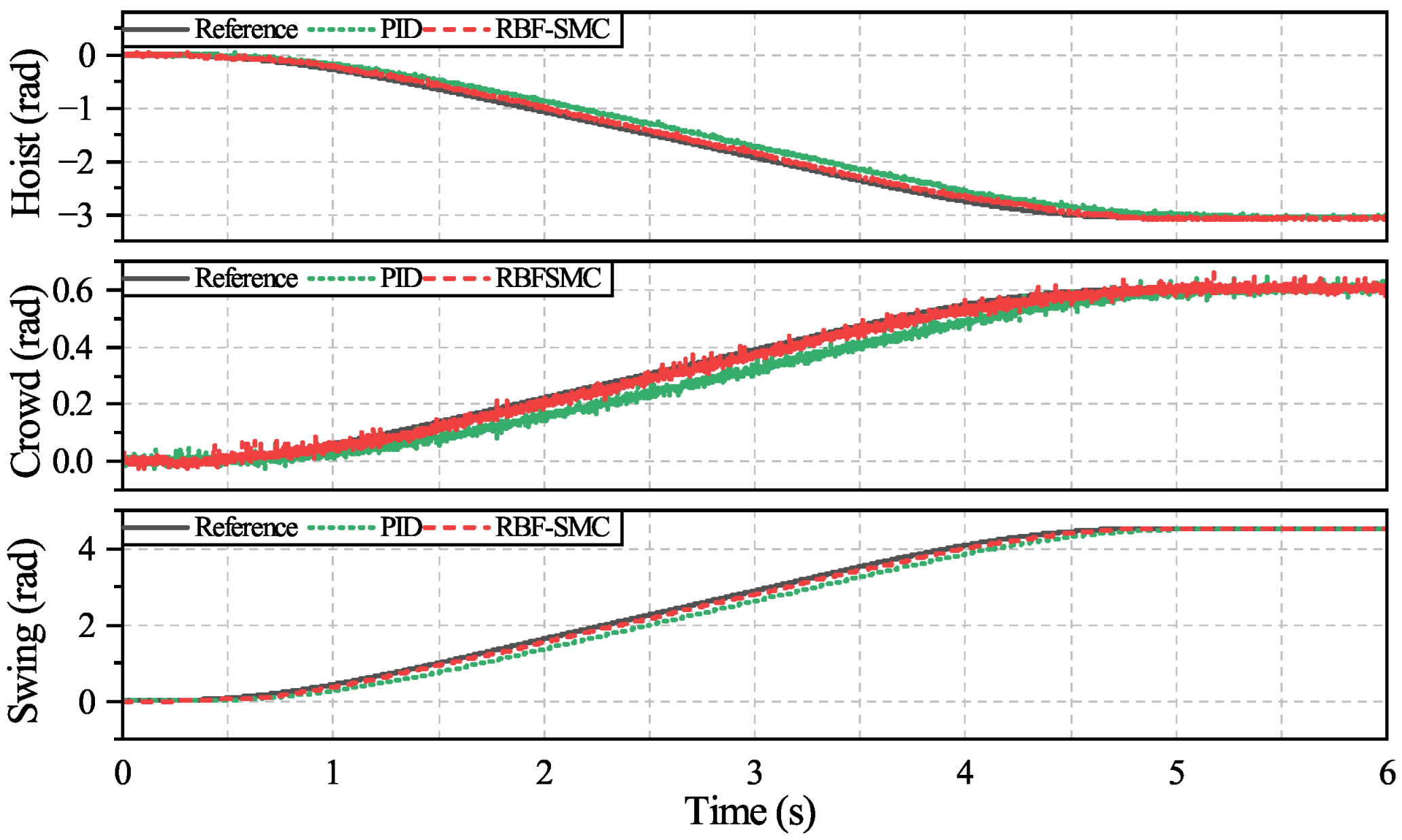
To verify the control performance of the proposed sliding-mode controller, the trajectory planning result of Condition 1 is selected as the reference trajectory for trajectory control experiments on the scaled experimental platform. The control performance is then compared with that of a traditional PID controller, as PID remains the most commonly adopted control strategy in industry owing to its straightforward structure and well-established tuning methods. PID parameters were tuned using the Ziegler–Nichols method and further manually refined for trajectory tracking tasks.The final gains were confirmed to be optimal under the given system dynamics, as further adjustments led to degraded performance or instability. According to the motion model, the values of $\theta$, d, $\alpha$ are converted into the rotation angles of the hoisting, crowding, and swing motors. The trajectory control results are shown in Figure 22 and Figure 23 and

Table 8. Trajectory control performance.

Maximum Instantaneous Error
	PID	RBF-SMC
Hoisting Motor	$270.1\times {10}^{-3}$	$147.0\times {10}^{-3}$
Crowding Motor	$105.1\times {10}^{-3}$	$56.5\times {10}^{-3}$
Swing Motor	$276.4\times {10}^{-3}$	$121.7\times {10}^{-3}$
Root Mean Square Error
	PID	RBF-SMC
Hoisting Motor	$152.62\times {10}^{-3}$	$61.61\times {10}^{-3}$
Crowding Motor	$49.37\times {10}^{-3}$	$17.45\times {10}^{-3}$
Swing Motor	$195.40\times {10}^{-3}$	$71.64\times {10}^{-3}$
Time Delay (s)
	PID	RBF-SMC
Hoisting Motor	$0.25$	$0.08$
Crowding Motor	$0.43$	$0.12$
Swing Motor	$0.22$	$0.08$

. The control performance is evaluated using a combination of maximum instantaneous error, root mean square error, and time delay, which together provide a more comprehensive assessment of transient deviation, steady-state accuracy, and dynamic responsiveness. Table 8 shows that the proposed RBF-SMC controller outperforms the traditional PID controller across all three motors. It significantly reduces the maximum instantaneous error, root mean square error, and time delay, indicating improved transient robustness, steady-state accuracy, and dynamic responsiveness. These results confirm that the RBF-SMC achieves more precise and timely trajectory tracking under various operating conditions.

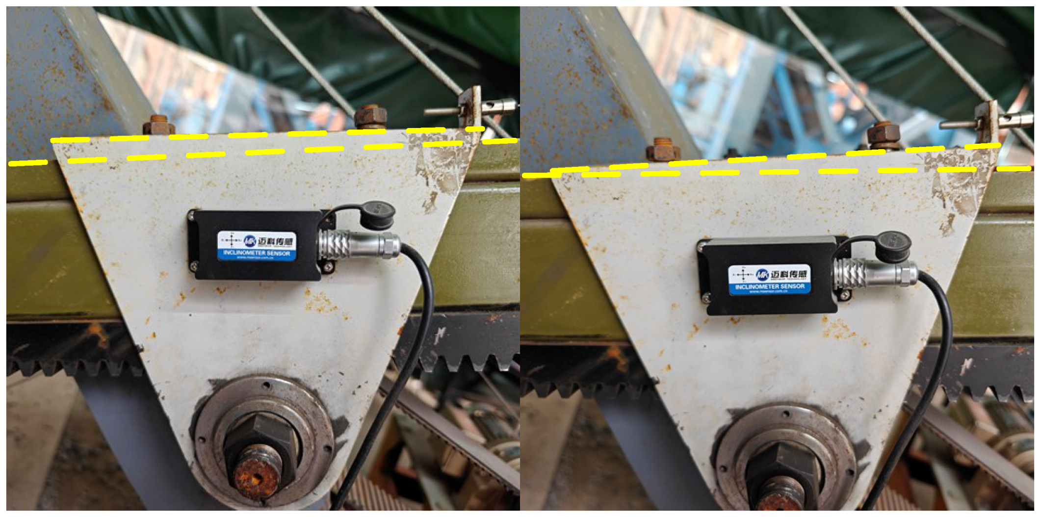
The disturbance observation results are shown in Figure 24 aligns with expectations. As the disturbance torque on the motor shaft is difficult to measure directly, we computed the theoretical disturbance under ideal conditions based on the reference trajectory of the motor motion, allowing a rough comparison with the observed values. It is important to note that for the estimated disturbance force in the crowding motion, manufacturing errors in the scaled-down test rig led to gear jamming between the crowding gear and rack, rather than simple misalignment. As illustrated in Figure 25, the jamming caused the crowding motor to stall intermittently and forced it to move in a stepwise manner by overcoming the resistance of each tooth. This resulted in a gradual increase in the overall estimated resistance force, along with localized fluctuations, particularly noticeable around 2 s and 5 s. This abnormal mechanical interaction ultimately resulted leading to discrepancies between the observed disturbance of the crowding motor and its ideal value.

The main parameters of RBF-SMC and the PID controller are shown in

Table 9. Parameters of the controllers.

		Hoisting	Crowding	Swing
	$k_p$	10	3	25
PID	$k_i$	$0.01$	$0.01$	$0.03$
	$k_d$	0	0	0
	c	5	20	10
RBF-SMC	$\eta$	10	6	12
	J	$2.26$	$24.6$	$37.9$

.

In general, the results demonstrate that the proposed RBF-SMC significantly improves system robustness against external disturbances. By effectively estimating and compensating for unknown input torques, the RBF network enables the controller to maintain higher tracking accuracy with reduced steady-state error and shorter time delay, even under varying load conditions. Compared to conventional control methods, the combined RBF-SMC strategy achieves smoother response and better disturbance rejection.

In addition, we observed that the controller also performs well under unexpected mechanical interferences, such as the backlash and resistance fluctuations caused by the rack and pinion. These observations further support the robustness of the proposed method in practical scenarios.

7. Conclusions

This paper presents a control framework for the autonomous swing and unloading operation of electric rope shovels, focusing on relative positioning, motion planning, and high-precision trajectory tracking.

A LiDAR-based positioning method is designed and tested through simulation experiments using two cargo containers to represent mining trucks. The algorithm successfully identified the nearest truck, with average Euclidean distance error of 24.51 mm, demonstrating its effectiveness.

Based on the positioning results, a trajectory planning method was developed to generate time-optimal motion trajectories for truck loading. Two scenarios were simulated: one without obstacles and one requiring obstacle avoidance. The planning algorithm successfully generated smooth and efficient trajectories in both cases.

The proposed RCRRBF network was validated through simulations, confirming its ability to accurately estimate external disturbances affecting motor control.

Finally, trajectory control experiments were conducted on a scaled-down test rig. The results showed that the RBF-SMC significantly outperformed PID control, effectively compensating for external disturbances and achieving high-precision control. The disturbance estimation results were consistent with theoretical expectations.

These findings confirm the feasibility of integrating LiDAR-based positioning, trajectory planning, and advanced control strategies for autonomous operations. Future research will focus on improving environmental adaptability and validating the approach on full-scale mining shovels to further advance intelligent mining automation.

Nonetheless, several limitations remain and point to future work. The current study is based on a scaled-down prototype and does not yet include full-scale field testing. Future work will focus on validating the proposed system under actual mining conditions, including real-time LiDAR-based positioning and trajectory planning that simultaneously considers obstacle avoidance for both the material pile and the truck body. In terms of motor control, an extended state observer (ESO) will be introduced to suppress sensor noise, allowing the sliding-mode controller to achieve even higher tracking accuracy. These enhancements aim to improve the system’s robustness and adaptability in complex, real-world excavation environments.

References

1. Chen, Z.; Yang, Y.; Zhou, L.; Hou, H.; Zhang, Y.; Liang, J.; Zhang, S. Ecological restoration in mining areas in the context of the Belt and Road initiative: Capability and challenges. Environ. Impact Assess. Rev. 2022, 95, 106767. [Google Scholar] [CrossRef]
2. Teng, S.; Li, L.; Li, Y.; Hu, X.; Li, L.; Ai, Y.; Chen, L. FusionPlanner: A multi-task motion planner for mining trucks via multi-sensor fusion. Mech. Syst. Signal Process. 2024, 208, 111051. [Google Scholar] [CrossRef]
3. Khorzoughi, M.B.; Hall, R. A Study of Digging Productivity of an Electric Rope Shovel for Different Operators. Minerals 2016, 6, 48. [Google Scholar] [CrossRef]
4. Ibrahim, M.A.; Hassan, G.; Hassanein, H.S.; Obaia, K. Wireless Sensing for Ground Engaging Tools. In Proceedings of the GLOBECOM 2020—2020 IEEE Global Communications Conference, Taipei, Taiwan, 7–11 December 2020; pp. 1–6. [Google Scholar] [CrossRef]
5. Qin, Z.; Chen, S.; Xu, X.; Zhao, M. Research on Key Technologies and System Construction of Smart Mine. In Proceedings of the 2020 5th Asia-Pacific Conference on Intelligent Robot Systems (ACIRS), Singapore, 17–19 July 2020; pp. 116–121. [Google Scholar] [CrossRef]
6. Xie, J.; Ge, F.; Cui, T.; Wang, X. A virtual test and evaluation method for fully mechanized mining production system with different smart levels. Int. J. Coal Sci. Technol. 2022, 9, 41. [Google Scholar] [CrossRef]
7. Zhang, J.; Yan, Q.; Zhu, X.; Yu, K. Smart industrial IoT empowered crowd sensing for safety monitoring in coal mine. Digit. Commun. Netw. 2023, 9, 296–305. [Google Scholar] [CrossRef]
8. Xie, J.; Yang, Z.; Wang, X.; Zeng, Q.; Li, J.; Li, B. A Virtual Reality Collaborative Planning Simulator and Its Method for Three Machines in a Fully Mechanized Coal Mining Face. Arab. J. Sci. Eng. 2018, 43, 4835–4854. [Google Scholar] [CrossRef]
9. Feng, C.; Shen, Y.; Wang, J.; Wang, Q.; Suo, Z.; Su, F. Task-unit based trajectory generation for excavators utilizing expert operator skills. Autom. Constr. 2024, 158, 105247. [Google Scholar] [CrossRef]
10. Feng, Y.; Wu, J.; Lin, B.; Guo, C. Excavating Trajectory Planning of a Mining Rope Shovel Based on Material Surface Perception. Sensors 2023, 23, 6653. [Google Scholar] [CrossRef]
11. Feng, H.; Jiang, J.; Ding, N.; Shen, F.; Yin, C.; Cao, D.; Li, C.; Liu, T.; Xie, J. Multi-objective time-energy-impact optimization for robotic excavator trajectory planning. Autom. Constr. 2023, 156, 105094. [Google Scholar] [CrossRef]
12. Fan, Z.; Zhang, T.; Qiao, J.; Li, G.; Zhao, Y.; Wang, X.; Sun, W.; Song, X. Multi-objective Excavation Trajectory Optimization for Intelligent Electric Shovel Based on ROS. IOP Conf. Ser. Mater. Sci. Eng. 2020, 717, 012015. [Google Scholar] [CrossRef]
13. Yao, Z.; Zhao, S.; Tan, X.; Wei, W.; Wang, Y. Real-time task-oriented continuous digging trajectory planning for excavator arms. Autom. Constr. 2023, 152, 104916. [Google Scholar] [CrossRef]
14. Zhang, Y.; Sun, Z.; Sun, Q.; Wang, Y.; Li, X.; Yang, J. Time-jerk optimal trajectory planning of hydraulic robotic excavator. Adv. Mech. Eng. 2021, 13, 1–13. [Google Scholar] [CrossRef]
15. Zhao, J.; Hu, Y.; Liu, C.; Tian, M.; Xia, X. Spline-Based Optimal Trajectory Generation for Autonomous Excavator. Machines 2022, 10, 538. [Google Scholar] [CrossRef]
16. Zhang, T.; Fu, T.; Cui, Y.; Song, X. Toward autonomous mining: Design and development of an unmanned electric shovel via point cloud-based optimal trajectory planning. Front. Mech. Eng. 2022, 17, 30. [Google Scholar] [CrossRef]
17. Wang, D.; Zheng, L.; Yu, H.; Zhou, W.; Shao, L. Robotic excavator motion control using a nonlinear proportional-integral controller and cross-coupled pre-compensation. Autom. Constr. 2016, 64, 1–6. [Google Scholar] [CrossRef]
18. Ding, H.; Sang, Z.; Li, Z.; Shi, J.; Wang, Y.; Meng, D. Trajectory planning and control of large robotic excavators based on inclination-displacement mapping. Autom. Constr. 2024, 158, 105209. [Google Scholar] [CrossRef]
19. Fan, R.; Li, Y.; Yang, L.; Qin, T.; Zhang, Y.; Wang, Z. Coordinated trajectory tracking control for mining excavator with oscillating external disturbance. J. Field Robot. 2024, 41, 258–272. [Google Scholar] [CrossRef]
20. Feng, H.; Yin, C.B.; Weng, W.W.; Ma, W.; Zhou, J.J.; Jia, W.H.; Zhang, Z.L. Robotic excavator trajectory control using an improved GA based PID controller. Mech. Syst. Signal Process. 2018, 105, 153–168. [Google Scholar] [CrossRef]
21. Ha, Q.; Nguyen, Q.; Rye, D.; Durrant-Whyte, H. Impedance control of a hydraulically actuated robotic excavator. Autom. Constr. 2000, 9, 421–435. [Google Scholar] [CrossRef]
22. Okada, T.; Yamamoto, T.; Doi, T.; Koiwai, K.; Yamashita, K. Database-driven model predictive control system for online adaptation of an autonomous excavator to environmental conditions. Control Eng. Pract. 2024, 145, 105843. [Google Scholar] [CrossRef]
23. Yaghini, A.; Hall, R.; Apel, D. Autonomous and Operator-Assisted Electric Rope Shovel Performance Study. Mining 2022, 2, 699–711. [Google Scholar] [CrossRef]
24. Dunbabin, M.; Corke, P. Autonomous Excavation Using a Rope Shovel. In Field and Service Robotics; Corke, P., Sukkariah, S., Eds.; Springer: Berlin/Heidelberg, Germany, 2006; pp. 555–566. [Google Scholar]
25. Li, Y.; Ibanez-Guzman, J. Lidar for Autonomous Driving: The Principles, Challenges, and Trends for Automotive Lidar and Perception Systems. IEEE Signal Process. Mag. 2020, 37, 50–61. [Google Scholar] [CrossRef]
26. Kuang, Z.; Gao, H.; Tomizuka, M. Precise Linear-Motor Synchronization Control via Cross-Coupled Second-Order Discrete-Time Fractional-Order Sliding Mode. IEEE-ASME Trans. Mechatron. 2021, 26, 358–368. [Google Scholar] [CrossRef]
27. Chandra, A.; Kurian, P.C.; Priya, P.S.L. Sliding-Mode High-Gain Observer based Position Control for an Electro-Hydraulic Actuator. In Proceedings of the 10th IEEE International Conference on Power Electronics, Drives and Energy Systems (IEEE PEDES), Jaipur, India, 14–17 December 2022. [Google Scholar] [CrossRef]
28. Feng, H.; Song, Q.Y.; Ma, S.L.; Ma, W.; Yin, C.B.; Cao, D.H.; Yu, H.F. A new adaptive sliding mode controller based on the RBF neural network for an electro-hydraulic servo system. ISA Trans. 2022, 129, 472–484. [Google Scholar] [CrossRef]
29. Liu, X.; Deng, Y.; Liu, J.; Cao, H.; Xu, C.; Liu, Y. Fixed-time integral terminal sliding mode control with an adaptive RBF neural network for PMSM speed regulation. Control Eng. Pract. 2025, 156, 106236. [Google Scholar] [CrossRef]
30. Panagi, P.; Polycarpou, M.M. Decentralized Fault Tolerant Control of a Class of Interconnected Nonlinear Systems. IEEE Trans. Autom. Control 2011, 56, 178–184. [Google Scholar] [CrossRef]
31. Li, X.; Ge, M.; Dai, X.; Ren, X.; Fritsche, M.; Wickert, J.; Schuh, H. Accuracy and reliability of multi-GNSS real-time precise positioning: GPS, GLONASS, BeiDou, and Galileo. J. Geod. 2015, 89, 607–635. [Google Scholar] [CrossRef]
32. Scott, M.T.U.; Scott, T.J.; Kelly, V.G. The Validity and Reliability of Global Positioning Systems in Team Sport: A Brief Review. J. Strength Cond. Res. 2016, 30, 1470–1490. [Google Scholar] [CrossRef]
33. Huang, S.; Gojcic, Z.; Usvyatsov, M.; Wieser, A.; Schindler, K. Predator: Registration of 3D Point Clouds With Low Overlap. In Proceedings of the IEEE/CVF Conference on Computer Vision and Pattern Recognition (CVPR), Nashville, TN, USA, 22–25 June 2021; pp. 4267–4276. [Google Scholar]
34. Bai, X.; Luo, Z.; Zhou, L.; Fu, H.; Quan, L.; Tai, C.L. D3Feat: Joint Learning of Dense Detection and Description of 3D Local Features. In Proceedings of the IEEE/CVF Conference on Computer Vision and Pattern Recognition (CVPR), Seattle, WA, USA, 13–19 June 2020. [Google Scholar]
35. Forstner, W.; Khoshelham, K. Efficient and Accurate Registration of Point Clouds With Plane to Plane Correspondences. In Proceedings of the IEEE International Conference on Computer Vision (ICCV) Workshops, Venice, Italy, 22–29 October 2017. [Google Scholar]
36. Rusu, R.B.; Cousins, S. 3D is here: Point Cloud Library (PCL). In Proceedings of the 2011 IEEE International Conference on Robotics and Automation, Shanghai, China, 9–13 May 2011; pp. 1–4. [Google Scholar] [CrossRef]
37. Bai, X.; Luo, Z.; Zhou, L.; Chen, H.; Li, L.; Hu, Z.; Fu, H.; Tai, C.L. PointDSC: Robust Point Cloud Registration Using Deep Spatial Consistency. In Proceedings of the IEEE/CVF Conference on Computer Vision and Pattern Recognition (CVPR), Nashville, TN, USA, 22–25 June 2021; pp. 15859–15869. [Google Scholar]
38. Kelly, M. An Introduction to Trajectory Optimization: How to Do Your Own Direct Collocation. SIAM Rev. 2017, 59, 849–904. [Google Scholar] [CrossRef]
39. Glennie, C. Rigorous 3D error analysis of kinematic scanning LIDAR systems. J. Appl. Geod. 2007, 1, 147–157. [Google Scholar] [CrossRef]
40. Zhang, J.; Singh, S. Low-drift and real-time lidar odometry and mapping. Auton. Robot. 2017, 41, 401–416. [Google Scholar] [CrossRef]
Figure 1. Electric rope shovel and mining truck.
Actuators 14 00394 g001
Figure 2. Cabin view of electric rope shovel.
Actuators 14 00394 g002
Figure 3. System workflow.
Actuators 14 00394 g003
Figure 4. Three-dimensional model of electric rope shovel.
Actuators 14 00394 g004
Figure 5. Excavation part of electric rope shovel.
Actuators 14 00394 g005
Figure 6. The mining truck approaching.
Actuators 14 00394 g006
Figure 7. Progress of LiDAR positioning.
Actuators 14 00394 g007
Figure 8. Positioning of the truck.
Actuators 14 00394 g008
Figure 9. RBF-based sliding-mode controller.
Actuators 14 00394 g009
Figure 10. Experimental Bench and Control System.
Actuators 14 00394 g010
Figure 11. Simulate mining trucks and positioning experiment.
Actuators 14 00394 g011
Figure 12. Point cloud and detected lines.
Actuators 14 00394 g012
Figure 13. Noise ratio under different parameters.
Actuators 14 00394 g013
Figure 14. The other two positions of the location experiment.
Actuators 14 00394 g014
Figure 15. Condition 1 of trajectory planning.
Actuators 14 00394 g015
Figure 16. Polynomial coefficient optimization process.
Actuators 14 00394 g016
Figure 17. Optimized trajectory.
Actuators 14 00394 g017
Figure 18. Condition 2 of trajectory planning.
Actuators 14 00394 g018
Figure 19. Polynomial coefficient optimization process with obstacle avoidance.
Actuators 14 00394 g019
Figure 20. Optimized trajectory with obstacle avoidance.
Actuators 14 00394 g020
Figure 21. Simulation experiment of RCRRBF.
Actuators 14 00394 g021
Figure 22. Control performance of motors by PID and RBF-SMC.
Actuators 14 00394 g022
Figure 23. Tracking error of PID and RBF-SMC.
Actuators 14 00394 g023
Figure 24. Disturbance observation of three motors.
Actuators 14 00394 g024
Figure 25. Misalignment between crowding gear-rack and saddle.
Actuators 14 00394 g025