Abstract
Given that grinding robots are easily affected by internal and external disturbances when machining complex surfaces with high precision, in this study, an adaptive robust impedance control method combining a radial basis function neural network (RBFNN) and sliding mode control (SMC) is proposed. In a Cartesian coordinate system, we first use the universal approximation ability of the RBFNN to accurately identify and actively compensate for complex unknown disturbances in robot dynamics online. Then, an improved sliding mode impedance controller, which uses robust sliding mode control to effectively suppress the influence of RBFNN identification error and residual disturbance on trajectory tracking and ensure the accuracy of impedance control, is implemented. This approach improves the control performance and overcomes the inherent chattering phenomenon of the traditional sliding mode.
1. Introduction
High-end equipment is the central focus of China’s industrial upgrading and manufacturing power strategy. The surface quality of high-end equipment components directly impacts both the performance and lifespan of equipment. Grinding processes can enhance the surface integrity of the workpiece, eliminate surface burrs, optimize surface roughness, and improve the fatigue strength of the workpiece. However, traditional manual grinding faces challenges, such as low efficiency and inconsistent quality. In contrast, robotic automated grinding offers high precision and excellent repeatability and has been widely adopted [1]. Nevertheless, the shapes and structures of workpieces are often complex, and control methods that solely focus on robot end position tracking may result in excessive contact forces. Such extreme contact forces can lead to surface wear or structural damage to the workpiece. Therefore, the design of controllers for complex surface grinding robots should prioritize dynamic adaptability in uncertain environments [2].
As a fundamental method of active compliance control, impedance control can dynamically adjust the interactive responses between a robot and a workpiece. When processing complex surfaces, impedance control effectively mitigates the process failures caused by errors in robot trajectory tracking [3,4]. Such process failures may include wear accumulation and surface burns on the workpiece. The existing impedance control methods encompass backstepping control [5,6], adaptive control [7], H-∞ control [8,9], etc. Based on traditional position impedance control, an earlier study [10] constructed an impedance controller based on environmental parameter identification by introducing the recursive least squares method with a forgetting factor to update environmental stiffness in real time online and correct the reference position to reduce the force tracking error. Another study [11] proposed a variable impedance control method for a continuous medium manipulator based on a finite-time observer. By identifying acceleration, it avoided the difficulty of directly sensing interference force and showed good robustness and stability in a noisy environment. A different study [12] investigated an adaptive tracking impedance control strategy for manipulators working within an uncertain contact environment. The proposed position and attitude controllers can ensure the finite-time convergence of state variables and do not require prior knowledge of the disturbance’s boundary. Furthermore, another group [13] proposed a whole-body impedance control method for a humanoid, wheeled robot that uses a fuzzy adaptive system to compensate for the uncertain dynamics of the controlled system. Moreover, a recent study [14] addressed the problem of stability being ignored in the design of variable impedance controllers for existing aerospace manipulators by implementing a variable impedance control system with state-independent stability to ensure the exponential stability of the desired variable impedance dynamic system. Impedance controllers based on mechanism models depend on accurate dynamic information regarding the robot. However, in grinding operations, factors such as friction force during tool–workpiece contact and the load change caused by material removal during grinding will cause the model to deviate from the real system.
Applying machine learning techniques to approximate unmodeled dynamics or load variations, as well as to rectify dynamic errors in real time, can enhance impedance control precision, while reducing controller dependence on the model parameters [15,16]. Radial basis function neural networks (RBFNNs), known for their superior accuracy and efficiency in identifying system nonlinearities, are widely utilized in robotic control systems [17,18]. A previous study [19] proposes a fully distributed control strategy that incorporates neural network-based task-space synchronization controllers and neural network-based null-space formation controllers. Another study [20] introduced a sliding mode control framework that employs neural networks for manipulators that are subject to system uncertainties, input dead zones, and external disturbances. In this context, the neural network estimates unknown parameters related to system uncertainty and input dead zones. A further study [21] presented an enhanced incremental radial basis function neural network designed to estimate the dynamic parameters of manipulators operating in constrained environments. Moreover, a recent study [22] outlined a methodology for grouping model parameters and training an RBF neural network that computes the average parameter values for each group as reference points and establishes relationships between the optimal controller feedback gains and the system parameters. Furthermore, another study [23] described an adaptive neural network tracking controller that utilizes full-state feedback via RBFNNs for unknown dynamic models, with a disturbance observer compensating for unidentified disturbances. It is important to note that the inherent identification errors in neural networks may lead to discrepancies between the estimated and actual dynamic model values, thereby affecting the accuracy of controller output torque calculations. Persistent and accumulating errors can induce system oscillations or divergence, ultimately compromising the robustness of the control algorithm.
Sliding mode control (SMC) is highly robust. Neural network identification errors can be considered bounded uncertainty within the framework of SMC, and the upper bound of this error can be directly compensated for by designing a sliding mode switching term. This approach ensures stable system convergence despite the presence of identification errors [24,25,26]. An earlier study [27] introduced a sliding mode control strategy based on RBF neural networks for T-S fuzzy descriptor systems that estimates system nonlinearities and unknown constants, while ensuring the fulfillment of system accessibility conditions. Another study [28] presented an RBF neural network-based sliding mode control strategy applied to steer-by-wire controller design that effectively enhanced the dynamic response of a steering system at the level needed for application in vehicles. To address the uncertainties in micro-electromechanical system (MEM) gyroscope systems, one study [29] employed radial basis function neural networks for approximation, establishing update rules for parameter vectors and RBFNN weights based on tracking errors and filtered modeling error data.
However, RBFNN identification error increases the sliding mode switching term value, leading to high-frequency chattering. Reaching laws can enhance the system’s dynamic performance by dynamically adjusting the reaching speed and smoothing the switching terms [30]. Some common reaching laws include the isokinetic approach law (IAL) and the exponential approach law (EAL). A previous study [31] introduced a novel variable exponential power reaching law that adaptively adjusts the reaching speed based on the initial state of the system and analyzed its finite-time convergence characteristics. Another study [32] proposed a fractional-order reaching law sliding mode controller with finite-time performance that significantly improved the system’s robustness and transient response, while ensuring finite-time convergence of the controller. A further study [33] developed a predefined variable power time reaching law that effectively reduces chattering, minimizes the control input, and strictly guarantees predefined time convergence.
Based on the analysis presented above, this study proposes an adaptive impedance control method that integrates machine learning with a sliding mode algorithm for a complex surface-grinding robot. The objective was to enhance the robot’s adaptability to intricate contact environments, thereby achieving more accurate and stable grinding results. The main contributions of this paper are as follows: (1) a novel adaptive disturbance identification method based on an RBFNN is developed to accurately estimate the uncertainties encountered by the robot during online grinding; (2) by leveraging the inherent robustness of sliding mode control, estimation errors and unmodeled dynamics are actively mitigated to ensure stable tracking of the desired impedance model dynamics in the presence of significant disturbances; (3) an exponential reaching law is introduced into the sliding mode control design, effectively reducing chattering and enhancing the interactive stability of free-form surface grinding, while maintaining robust convergence.
The remainder of this paper is organized as follows: In the second section, we establish the impedance control model based on a dynamic model of the robot in a joint coordinate system. The third section presents an adaptive neural network impedance control method designed to address the various disturbances encountered by the grinding robot, along with proof of its stability. In the fourth section, we present the results from simulation analyses and experimental verification. Finally, a summary is provided in the fifth section.
2. Description of the Grinding Robot Impedance Dynamics
Task space models are frequently employed in the design of impedance controllers for robots, as they can directly represent impedance between the grinding device and the workpiece. This approach eliminates the need for joint space models in controller design, thereby reducing the computational burden and minimizing the control errors. Taking into account external disturbances and modeling uncertainties, the robot dynamics model utilizes joint angles as variables [2].
in which is the angular displacement of the robot joints, is the joint control torque applied by the actuators, is the symmetric positive definite inertia matrix, is the centrifugal and Coriolis force matrixes, is the gravity vector, and is the external disturbance.
Let be the position vector of the robot end-effector, which is a function of joint angle . Mapping between and satisfies [14].
in which is the robot Jacobian matrix.
Let the contact force between the robot end-effector and the environment be .The dynamics equation is [22] given as follows:
in which is the desired end-effector trajectory, and is the actual end-effector trajectory. When a deviation occurs between them, a corresponding force is generated. are the mass, damping, and stiffness coefficient matrices, respectively.
At equilibrium, the relationship between the end-effector force and joint torque follows on from the virtual work principle [22].
Thus, the end-effector position-based impedance dynamics model is established [22]:
in which is the error and disturbance in modeling, ,
To facilitate the design of control methods, we make the following assumptions about the robot’s dynamics.
Assumption 1:
The inertia matrix is symmetric positive definite, uniformly bounded, and continuous, and its inverse exists, satisfying the following equation:
Assumption 2:
is skew-symmetric for any vector , satisfying the following equation:
In the actual grinding process, the desired end-effector trajectory may become unreachable, for example due to obstacles. Therefore, the goal of impedance control is to make the actual end-effector trajectory track the desired impedance trajectory , where the relationship between and is [22] given as follows:
where and .
3. Controller Design and Stability Analysis
Using an RBFNN to identify a grinding robot dynamic model can reduce the algorithm’s dependence on model parameters. In addition, constraining identification errors by using sliding mode control can enhance the algorithm’s robustness.
3.1. RBFNN
An RBF neural network is a three-layer network consisting of an input layer, a hidden layer, and an output layer. It uses radial basis functions as activation functions in the hidden layer to perform nonlinear transformation from the input layer to the hidden layer, while linear transformation is applied from the hidden layer to the output layer.
An RBF neural network is used for the function approximation of , and the network algorithm is [28] given as follows:
where is the network input, is the j-th node in the network’s hidden layer, is the output of the Gaussian function, is the ideal weight of the network, and is the approximation error of the network, .
The actual value identified by the RBF network is [28] given as follows:
where is the actual value of , and is the actual value of the network weight .
3.2. Adaptive Robust Impedance Control Method for a Grinding Robot Integrating an RBFNN and Sliding Mode
A block diagram of the control algorithm designed in this paper is presented below, as shown in Figure 1.
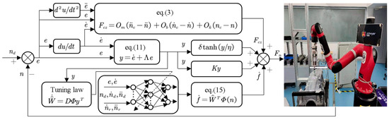
Figure 1.
Control algorithm block diagram.
Setting the position error of the end-effector of the grinding robot in the Cartesian coordinate system,
where is the desired impedance trajectory, and is the actual end-effector trajectory.
The linear sliding mode surface is defined as [24] follows:
where . From Equations (5) and (11), the following can be derived:
where .
Given this definition
Then
According to the RBF universal approximation theorem, an RBF neural network can be used to approximate .
Let the approximation value of , denoted as , be defined as follows:
where , D is the matrix to be designed, and .
Based on the above, an impedance controller was designed based on an RBFNN and the exponential approaching law:
where is the contact resistance compensation, is a robust term incorporating a hyperbolic tangent function to overcome system errors, and .
3.3. Stability Analysis
Substituting Equations (9) and (16) into (12) yields the following:
The Lyapunov function is defined as follows:
where and .
Then,
Substituting Equation (17) into the above equation yields the following:
Based on Assumption 2, the following can be concluded:
since
thus,
Only when , . According to the LaSalle invariance principle, the closed-loop system is asymptotically stable, meaning that as , y→0.
4. Simulation Analysis and Verification
The two-degree-of-freedom robotic hand and environmental contact model used in the simulation are shown in Figure 2.
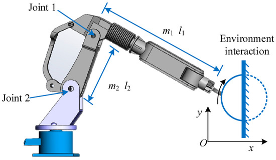
Figure 2.
Two-degrees-of-freedom robotic arm and environmental contact model.
The dynamic equation of the grinding robot with the end position as the variable is shown in Equation (5), specifically expressed as follows:
The system parameters of the robot used in the simulation are as follows:
The Jacobian matrix parameters describing the relationship between the velocity of the end-effector tip and the robot joint angular velocities are given as follows:
In the formula, the value of is given by , where
where represents the load, and are the lengths of joint 1 and joint 2, respectively, and is the acceleration of gravity, .
The actual parameters of the robot are shown in Table 1.

Table 1.
Robot parameter table.
The impedance parameters are as follows:
To validate the effectiveness of the proposed method, two simulation cases were conducted. The first case investigates the tracking performance for reference trajectories, while the second performs comparative analysis between the proposed method and two established existing methods. The first algorithm involves exponential reaching law-based sliding mode impedance control (ERL-SMC), the second algorithm involves an RBFNN and isokinetic approach law-based sliding mode impedance control (RBFNN-IAL-SMC), and the third algorithm corresponds to the novel method proposed in this work, which combines the RBFNN with the exponential reaching law in sliding mode impedance control (RBFNN-ERL-SMC). The RBFNN-ERL-SMC algorithm expression follows Equation (16).
Case1:
The desired trajectory is specified as an elliptical path for the robot’s end-effector, and this path is described by the equation , . The initial values of the robot desired end-effector trajectory and desired impedance trajectory are set as and , with initial values for the desired impedance trajectory given by and . To verify the ability of the proposed control method to eliminate steady-state tracking errors, the initial values of the robot end-effector are given as , which are distinct from the initial values of the desired impedance trajectory. To validate the robustness of the proposed method against disturbances, a time-varying disturbance is implemented; no disturbance is applied during s, while a defined disturbance is introduced for s. The contact surface of the obstacle is at .
The RBFNN parameters were set as follows:
The control algorithm parameters are shown in Table 2.
Table 2.
Control algorithm parameter table for case1.
During the simulation, the amplitude of estimation error in the x-direction and y-direction does not exceed 20 and 50 units, respectively, while maintaining stability. Therefore, the gains of the sliding mode robust term in the controller are designed as 20 and 50, which serve to suppress the estimation error of the RBFNN.
The tracking performance of the proposed method for the elliptic reference trajectory in the X-direction is shown in Figure 3 and Figure 4, while its performance in the Y-direction under the same trajectory is shown in Figure 5 and Figure 6. For the X-direction, the initial value of the robot’s actual end-effector trajectory is set at 0.5 cm, while the desired impedance trajectory initiates at 0.8 cm, specifically to preclude a performance validation compromise that could arise from identical starting conditions. Figure 3 demonstrates that the actual trajectory achieves exact tracking of the desired impedance trajectory in the X-direction at t = 0.5 s using the proposed control method. As demonstrated in Figure 4, the steady-state tracking error in the X-direction is maintained below 0.0092 cm during all the stabilization phases post t = 0.5 s. As shown in Figure 4, periodic oscillations occurred in the actual trajectory at t = 5 s. This phenomenon was caused by the external disturbance applied to the robot, where the disturbance signal took the form of a sawtooth wave function. Under the controller’s action, the robot is still able to remain stable during operation. Building upon the preceding tracking performance analysis, Figure 5 demonstrates accelerated convergence in the Y-direction using the proposed controller, achieving precise trajectory alignment at t = 0.6 s. Figure 6 confirms sustained steady-state tracking precision with errors constrained below 0.0075 cm, validating the robust disturbance rejection capabilities.
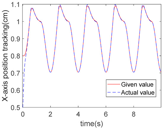
Figure 3.
X-direction tracking for elliptic trajectory: RBFNN-ERL-SMC.
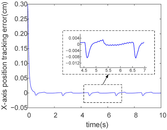
Figure 4.
X-direction tracking error for elliptic trajectory: RBFNN-ERL-SMC.
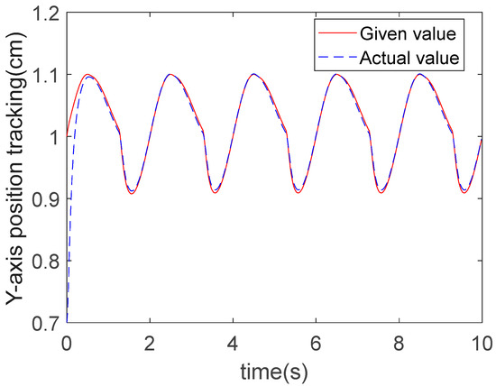
Figure 5.
Y-direction tracking for elliptic trajectory: RBFNN-ERL-SMC.
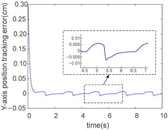
Figure 6.
Y-direction tracking error for elliptic trajectory: RBFNN-ERL-SMC.
In the proposed method of this paper, the RBFNN is employed for online disturbance estimation and real-time compensation, thereby reducing the control scheme’s dependence on the model parameters. Figure 7 and Figure 8 display the sums of the nine weight magnitudes in the X-direction network and the Y-direction network, respectively. As observed from these figures, the weights reach steady-state values around t = 0.5 s, indicating that the RBFNN has achieved convergence in disturbance estimation. This is consistent with the tracking performance of the robot’s end-effector trajectory.
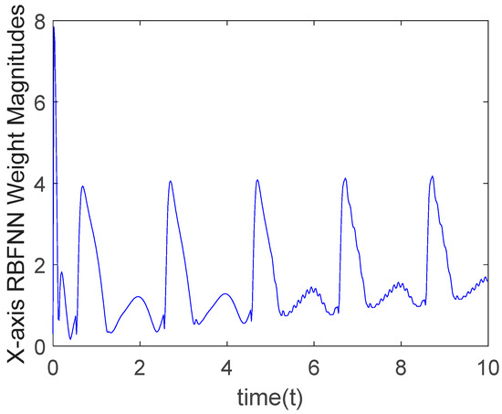
Figure 7.
The sum of the nine weight magnitudes in the X-direction.
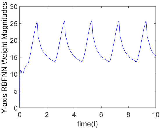
Figure 8.
The sum of the nine weight magnitudes in the Y-direction.
Case2:
To further validate the efficacy of the proposed method, two additional algorithms were adopted for comparative simulation. The desired trajectory of the robot’s end-effector is a circle, described by the equation , , and is applied. The control algorithm parameters are shown in Table 3. The parameters of the RBFNN remain consistent with those defined in case1.
Table 3.
Control algorithm parameter table for case 2.
The ERL-SMC algorithm expression is given as follows:
The RBFNN-IAL-SMC algorithm expression is given as follows:
The X-direction trajectory tracking results of the three algorithms for a circular trajectory are presented in Figure 9, Figure 10 and Figure 11. It can be observed from these figures that under the action of the controllers, the motion of the robot end-effector in the X-direction reached a steady state and successfully achieved accurate tracking of the given values. Specifically, the convergence time of ERL-SMC is 0.6 s, that of RBFNN-IAL-SMC is 0.45 s, and that of RBFNN-ERL-SMC is 0.4 s. The tracking errors for all three methods are shown in Figure 12, revealing an absolute error amplitude of 0.02 cm for the ERL-SMC method, 0.01 cm for RBFNN-IAL-SMC, and 0.005 cm for the proposed RBFNN-ERL-SMC. The comparative analysis of the control performance difference between these two methods in the X-direction is presented in Table 4.
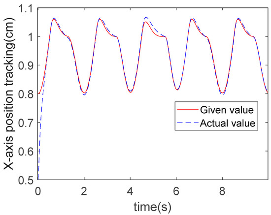
Figure 9.
X-direction tracking for circle trajectory: ERL-SMC.
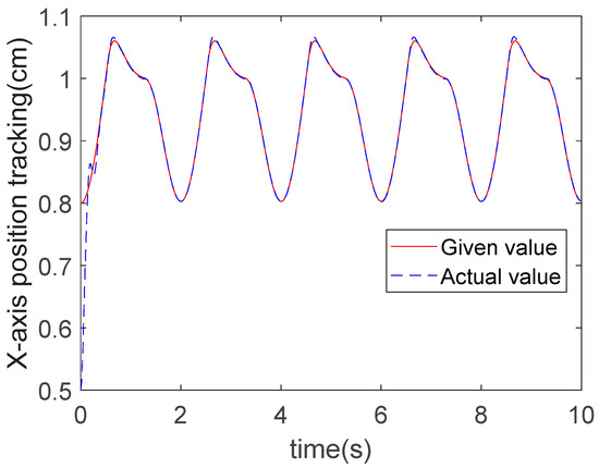
Figure 10.
X-direction tracking for circle trajectory: RBFNN-IAL-SMC.
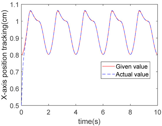
Figure 11.
X-direction tracking for circle trajectory: RBFNN-ERL-SMC.
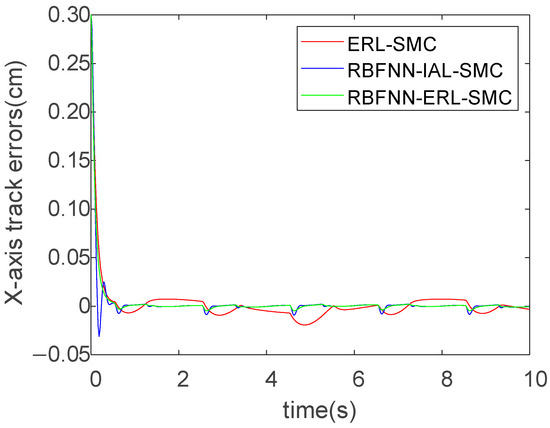
Figure 12.
X-direction tracking errors for all three methods.
Table 4.
Comparison of steady-state errors.
The results from the three algorithms in terms of Y-direction trajectory tracking are shown in Figure 13, Figure 14 and Figure 15. It can be observed from the figures that under the action of the controllers, the motion of the robot end-effector in the Y-direction reached a steady state and successfully achieved accurate tracking of the given values. Specifically, the convergence time of ERL-SMC was 0.5 s, that of RBFNN-IAL-SMC was 0.4 s, and that of RBFNN-ERL-SMC was 0.4 s. These results demonstrate that the implementation of the RBFNN significantly enhances the convergence speed. The tracking errors for all three methods are shown in Figure 16, revealing an absolute error amplitude of 0.015 cm for the ERL-SMC method, 0.011 cm for RBFNN-IAL-SMC, and 0.008 cm for the proposed RBFNN-ERL-SMC. The comparative analysis of the control performance difference between these two methods in the Y-direction is presented in Table 4.
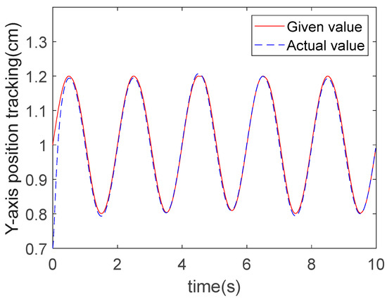
Figure 13.
Y-direction trajectory tracking of ERL-SMC.
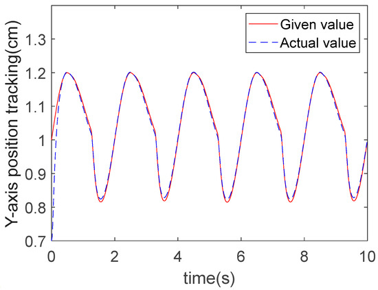
Figure 14.
Y-direction trajectory tracking of RBFNN-IAL-SMC.
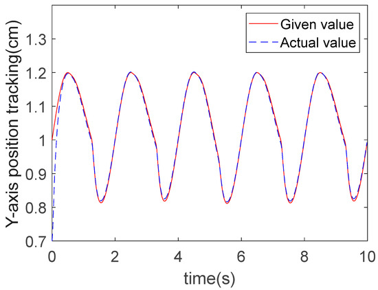
Figure 15.
Y-direction trajectory tracking of RBFNN-ERL-SMC.
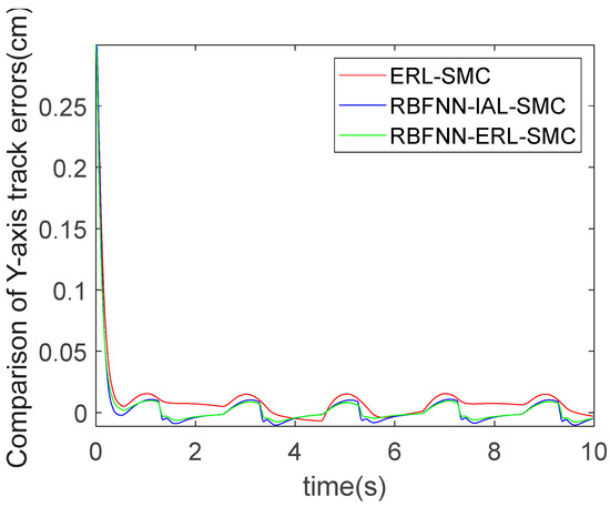
Figure 16.
Y-direction tracking errors for all three methods.
The tracking performances of the ideal trajectory, impedance trajectory, and actual trajectory of the robot end-effector in Cartesian space for the three algorithms are shown in Figure 17, Figure 18 and Figure 19. Using the proposed RBFNN-ERL-SMC method, the actual trajectory exhibits significantly smaller fluctuations compared to the other two simulations, with more concentrated trajectory paths and a superior performance.
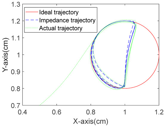
Figure 17.
Ideal position and actual position tracking of ERL-SMC.
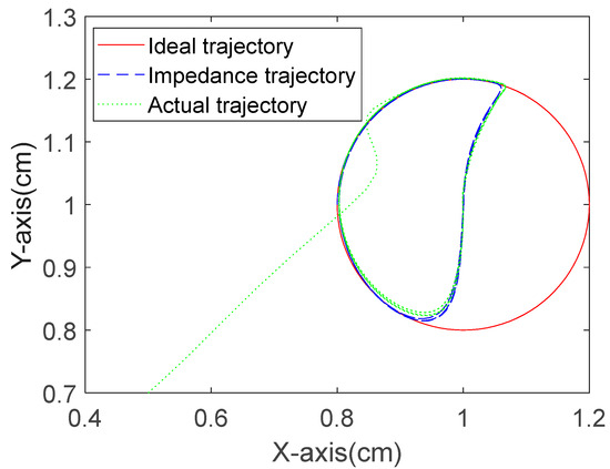
Figure 18.
Ideal position and actual position tracking of RBFNN-IAL-SMC.
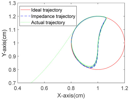
Figure 19.
Ideal position and actual position tracking of RBFNN-ERL-SMC.
To more intuitively demonstrate the control effects of these three simulations, the steady-state errors of the three control methods are compared in tabular form. The selected error metrics were the mean absolute error (MAE) and the root mean square error (RMSE), calculated as follows:
Table 4 shows that the RBFNN-ERL-SMC method outperforms both ERL-SMC and RBFNN-IAL-SMC. The proposed method reduces the MAE of the X-direction position from 0.00899 to 0.00404 and the MAE of the Y-direction position from 0.01175 to 0.00821. Furthermore, it reduces the RMSE of the X-direction position from 0.02658 to 0.02366 and the RMSE of the Y-direction position from 0.03057 to 0.02669.
5. Experimental Verification and Analysis
This section further examines the performance of the designed impedance control method through experimental verification and analysis. Figure 20 shows the grinding robot experimental system, which includes a Sawyer robot, a torque sensor, a high-speed electric spindle, a grinding head, and an engine block. This experiment compared the ERL-SMC and RBFNN-ERL-SMC controllers. Under the action of the controllers, all the joints achieved stable operation.
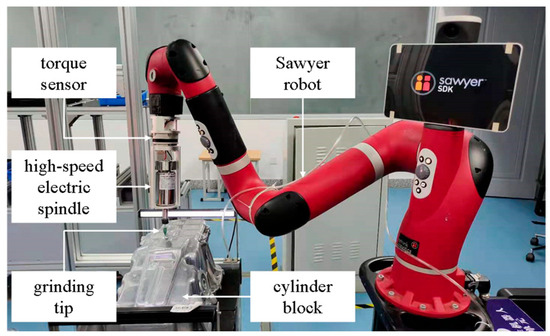
Figure 20.
Grinding robot experimental system.
The results for trajectory tracking in the X- and Y-directions by the two algorithms are shown in Figure 21, Figure 22, Figure 23, and Figure 24, respectively. Under the action of the controllers, the motion of the robot end-effector in the X-direction reached a steady state and achieved accurate tracking of the given values. From Figure 21, position tracking by ERL-SMC fluctuated from −30.18 mm to 133.54 mm in the X-direction, while with RBFNN-ERL-SMC it ranged from −29.69 mm to 129.98 mm. From Figure 23, in the Y-direction, ERL-SMC fluctuated from −547 mm to −501.5 mm, while with RBFNN-ERL-SMC, the fluctuation ranged from −547.5 mm to −502.7 mm. Critically, Figure 22 reveals that the steady-state error magnitude in the X-direction was reduced from 4.03 mm with ERL-SMC to 3.27 mm using RBFNN-ERL-SMC. Similarly, Figure 24 demonstrates Y-direction error reduction from 1.96 mm to 1.67 mm through RBFNN-ERL-SMC enhancement. This indicates that the system exhibited smaller fluctuations and more precise tracking using the RBFNN-ERL-SMC method.
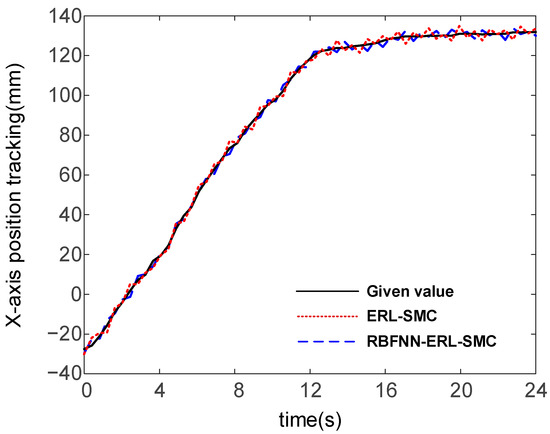
Figure 21.
X-direction position tracking.
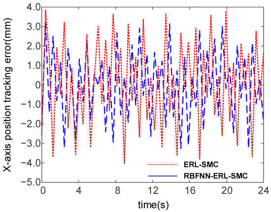
Figure 22.
X-direction position tracking error.
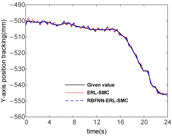
Figure 23.
Y-direction position tracking.
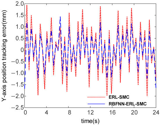
Figure 24.
Y-direction position tracking error.
6. Conclusions
This study investigated the limitations of traditional SMC in the context of environmental and model uncertainties within a Cartesian coordinate framework. To address these challenges, an impedance control method incorporating an RBFNN was proposed. Initially, the contact force was calculated based on the impedance parameters of the grinding system, as well as the position, velocity, and acceleration errors between the robot’s end-effector and its desired trajectory. This contact force was then utilized to transform the desired trajectory into an executable impedance trajectory for the robot. Subsequently, an RBFNN-based impedance control strategy was employed to track this impedance trajectory. The proposed method achieved convergence. Notably, under identical conditions and with a lower robust gain coefficient compared to traditional SMC, both the peak-to-peak trajectory tracking error and the convergence time were smaller than those of the traditional SMC method. Furthermore, the effectiveness of reaching laws was examined and verified. It was found that the exponential reaching law more effectively reduced the system’s steady-state error and enhanced the control precision of the robot’s end-effector compared to the constant velocity reaching law. Additionally, an appropriately selected proportional gain ensured system stability, while maintaining a rapid response. The stability of the control system was rigorously proven using Lyapunov’s stability theory. The primary objective of this control scheme was to ensure accurate tracking of the impedance trajectory by the actual trajectory. Our simulation and experimental results conclusively demonstrated that the proposed RBFNN-based impedance control method was highly robust in the face of environmental disturbances and system model uncertainties. Moreover, compared to the traditional SMC method, it produced a smaller steady-state error and higher control precision.
Author Contributions
Conceptualization, L.J.; data curation, K.C.; formal analysis, Z.L.; funding acquisition, L.J.; investigation, M.C.; methodology, K.C.; project administration, L.J.; resources, L.J., Z.L. and M.C.; software, K.C.; supervision, M.C.; validation, A.Q.; writing—original draft, K.C.; writing—review and editing, L.J. All authors have read and agreed to the published version of the manuscript.
Funding
This research was funded by National Natural Science Foundation of China (62303178, 62173137), Hunan Provincial Natural Science Foundation of China (2024JJ7139). The APC was funded by National Natural Science Foundation of China.
Institutional Review Board Statement
Not applicable.
Informed Consent Statement
Not applicable.
Data Availability Statement
The original contributions presented in the study are included in the article, further inquiries can be directed to the corresponding author.
Conflicts of Interest
Author Mingjian Cao was employed by the company Guoneng Baoshen. Railway Group Co., Ltd. The remaining authors declare that the research was conducted in theabsence of any commercial or financial relationships that could be construed as a potential conflict of interest.
References
- Li, C.; Zhao, L.; Xu, Z. Finite-time adaptive event-triggered control for robot manipulators with output constraints. IEEE Trans. Circuits Syst. II Express Briefs 2022, 69, 3824–3828. [Google Scholar] [CrossRef]
- Zhang, M.; Tong, W.; Li, P.; Hou, Y.; Xu, X.; Zhu, L.; Wu, E.Q. Robust neural dynamics method for redundant robot manipulator control with physical constraints. IEEE Trans. Ind. Inform. 2023, 19, 11721–11729. [Google Scholar] [CrossRef]
- Huang, H.C.; Chen, Y.X. Evolutionary optimization of fuzzy reinforcement learning and its application to time-varying tracking control of industrial parallel robotic manipulators. IEEE Trans. Ind. Inform. 2023, 19, 11712–11720. [Google Scholar] [CrossRef]
- Kim, H.; Oh, C.; Jang, I.; Park, S.; Seo, H.; Kim, H.J. Learning and generalizing cooperative manipulation skills using parametric dynamic movement primitives. IEEE Trans. Autom. Sci. Eng. 2022, 19, 3968–3979. [Google Scholar] [CrossRef]
- Ai, Y.; Wang, H. Fixed-time anti-synchronization of unified chaotic systems via adaptive backstepping approach. IEEE Trans. Circuits Syst. II Express Briefs 2022, 70, 626–630. [Google Scholar] [CrossRef]
- Ye, H.; Song, Y. Backstepping design embedded with time-varying command filters. IEEE Trans. Circuits Syst. II Express Briefs 2022, 69, 2832–2836. [Google Scholar] [CrossRef]
- Zhu, Y.; Zhu, W.; Liu, J.; Wang, Q.-G.; Yu, J. Command-filtered finite-time fuzzy adaptive fault-tolerant control of output-constrained robotic manipulators with unknown dead-zones. IEEE Trans. Circuits Syst. II Express Briefs 2023, 70, 2939–2943. [Google Scholar] [CrossRef]
- Golestani, M.; Chhabra, R.; Esmaeilzadeh, M. Finite-time nonlinear H∞ Control of robot manipulators with prescribed performance. IEEE Control Syst. Lett. 2023, 7, 1363–1368. [Google Scholar] [CrossRef]
- Wu, J.; Lian, B.; Su, H.; Zhu, Y. Data-Driven Weighted H Control of Persistent Dwell Time Switched Systems with Optimal Disturbance Attenuation Guaranteed. IEEE Trans. Autom. Sci. Eng. 2025, 22, 8162–8173. [Google Scholar] [CrossRef]
- Cai, J.; Wen, C.; Xing, L.; Yan, Q. Decentralized backstepping control for interconnected systems with non-triangular structural uncertainties. IEEE Trans. Autom. Control 2022, 68, 1692–1699. [Google Scholar] [CrossRef]
- Liang, X.; He, G.; Su, T.; Wang, W.; Huang, C.; Zhao, Q.; Hou, Z.-G. Finite-time observer-based variable impedance control of cable-driven continuum manipulators. IEEE Trans. Hum.-Mach. Syst. 2021, 52, 26–40. [Google Scholar] [CrossRef]
- Liang, J.; Zhong, H.; Wang, Y.; Chen, Y.; Zeng, J.; Mao, J. Adaptive force tracking impedance control for aerial interaction in uncertain contact environment using barrier function. IEEE Trans. Autom. Sci. Eng. 2024, 21, 4720–4731. [Google Scholar] [CrossRef]
- Bergeling, C.; Pates, R.; Rantzer, A. H-infinity optimal control for systems with a bottleneck frequency. IEEE Trans. Autom. Control 2020, 66, 2732–2738. [Google Scholar] [CrossRef]
- Liang, J.; Wang, Y.; Zhong, H.; Chen, Y.; Li, H.; Mao, J.; Wang, W. Robust variable impedance control for aerial compliant interaction with stability guarantee. IEEE Trans. Ind. Inform. 2023, 20, 3351–3360. [Google Scholar] [CrossRef]
- Cai, M.; Wang, Y.; Wang, S.; Wang, R.; Tan, M. Autonomous manipulation of an underwater vehicle-manipulator system by a composite control scheme with disturbance estimation. IEEE Trans. Autom. Sci. Eng. 2023, 21, 1012–1022. [Google Scholar] [CrossRef]
- Fan, Y.; Zhu, Z.; Li, Z.; Yang, C. Neural adaptive with impedance learning control for uncertain cooperative multiple robot manipulators. Eur. J. Control. 2023, 70, 100769. [Google Scholar] [CrossRef]
- She, Y.; Li, S.; Xin, M. Quantum-interference artificial neural network with application to space manipulator control. IEEE Trans. Aerosp. Electron. Syst. 2021, 57, 2167–2182. [Google Scholar] [CrossRef]
- Cao, S.; Sun, L.; Jiang, J.; Zuo, Z. Reinforcement learning-based fixed-time trajectory tracking control for uncertain robotic manipulators with input saturation. IEEE Trans. Neural Netw. Learn. Syst. 2021, 34, 4584–4595. [Google Scholar] [CrossRef] [PubMed]
- Li, Y.; Wang, L.; Liu, K.; He, W.; Yin, Y.; Johansson, R. Distributed neural-network-based cooperation control for teleoperation of multiple mobile manipulators under round-robin protocol. IEEE Trans. Neural Netw. Learn. Syst. 2021, 34, 4841–4855. [Google Scholar] [CrossRef] [PubMed]
- Zhang, Y.; Kong, L.; Zhang, S.; Yu, X.; Liu, Y. Improved sliding mode control for a robotic manipulator with input deadzone and deferred constraint. IEEE Trans. Syst. Man Cybern. Syst. 2023, 53, 7814–7826. [Google Scholar] [CrossRef]
- Guo, K.; Su, H.; Yang, C. A small opening workspace control strategy for redundant manipulator based on RCM method. IEEE Trans. Control Syst. Technol. 2022, 30, 2717–2725. [Google Scholar] [CrossRef]
- Yang, Y.; Wu, X.; Song, B.; Li, Z. Whole-body fuzzy based impedance control of a humanoid wheeled robot. IEEE Robot. Autom. Lett. 2022, 7, 4909–4916. [Google Scholar] [CrossRef]
- Huo, Y.; Li, X.; Zhang, X.; Li, X.; Sun, D. Adaptive intention-driven variable impedance control for wearable robots with compliant actuators. IEEE Trans. Control Syst. Technol. 2022, 31, 1308–1323. [Google Scholar] [CrossRef]
- Zhai, J.; Li, Z. Fast-exponential sliding mode control of robotic manipulator with super-twisting method. IEEE Trans. Circuits Syst. II Express Briefs 2022, 69, 489–493. [Google Scholar] [CrossRef]
- He, X.; Li, X.; Song, S. Nonsingular terminal sliding-mode control of second-order systems subject to hybrid disturbances. IEEE Trans. Circuits Syst. II Express Briefs 2022, 69, 5019–5023. [Google Scholar] [CrossRef]
- Nguyen, N.P.; Oh, H.; Moon, J. Continuous nonsingular terminal sliding-mode control with integral-type sliding surface for disturbed systems: Application to attitude control for quadrotor UAVs under external disturbances. IEEE Trans. Aerosp. Electron. Syst. 2022, 58, 5635–5660. [Google Scholar] [CrossRef]
- Li, R.; Yang, Y. Sliding-mode observer-based fault reconstruction for TS fuzzy descriptor systems. IEEE Trans. Syst. Man Cybern. Syst. 2021, 51, 5046–5055. [Google Scholar] [CrossRef]
- Gao, S.; Wang, J.; Guan, C.; Zhou, Z.; Liu, Z. Dynamic Characteristic Modeling and RBF-SMC Based Torque Control of a Novel Torque Vectoring Drive-axle for Electric Vehicles. IEEE Trans. Veh. Technol. 2025, 74, 5757–5770. [Google Scholar] [CrossRef]
- Zhang, R.; Xu, B.; Wei, Q.; Yang, T.; Zhao, W.; Zhang, P. Serial-parallel estimation model-based sliding mode control of MEMS gyroscopes. IEEE Trans. Syst. Man Cybern. Syst. 2021, 51, 7764–7775. [Google Scholar] [CrossRef]
- Zhang, Z.; Yang, X.; Wang, W.; Chen, K.; Cheung, N.C.; Pan, J. Enhanced sliding mode control for PMSM speed drive systems using a novel adaptive sliding mode reaching law based on exponential function. IEEE Trans. Ind. Electron. 2024, 71, 11978–11988. [Google Scholar] [CrossRef]
- Wang, Y.; Jiao, W. Fixed-time Disturbance Observer-Based Terminal Sliding Mode Control for Manipulators with a Novel Reaching Law. IEEE Access 2024, 12, 105766–105777. [Google Scholar] [CrossRef]
- Stihi, S.; Fareh, R.; Khadraoui, S.; Bettayeb, M. Tracking Finite-Time Prescribed Performance Fractional Power Rate Reaching Law Sliding-Mode Control For a 4-DOF Robot Manipulator. IEEE/ASME Trans. Mechatron. 2025, 30, 1236–1247. [Google Scholar] [CrossRef]
- Tao, R.; Ding, Y.; Yue, X.; Wu, N. A Predefined-time Non-singular Terminal Sliding Mode Control for Multi Space Transport Robot System with Varying Power Reaching Law. IEEE Trans. Aerosp. Electron. Syst. 2024, 60, 7886–7902. [Google Scholar] [CrossRef]


Disclaimer/Publisher’s Note: The statements, opinions and data contained in all publications are solely those of the individual author(s) and contributor(s) and not of MDPI and/or the editor(s). MDPI and/or the editor(s) disclaim responsibility for any injury to people or property resulting from any ideas, methods, instructions or products referred to in the content. |
© 2025 by the authors. Licensee MDPI, Basel, Switzerland. This article is an open access article distributed under the terms and conditions of the Creative Commons Attribution (CC BY) license (https://creativecommons.org/licenses/by/4.0/).