Adaptive Shared Trajectory Tracking Control for Output-Constrained Euler–Lagrange Systems

Abstract

This study presents the state-feedback and output-feedback adaptive shared trajectory tracking control laws for nonlinear Euler–Lagrange systems subject to parametric uncertainties and output constraints framed within linear inequalities. The logarithm-driven coordinate transformation is used to ensure that system outputs are consistently bounded by defined regions, while model-based adaptive laws are used in the machine controller to estimate and cancel parametric uncertainties and the human controller can be given arbitrarily. The stability of the whole controlled system is proved by Lyapunov stability theory, and simulation examples are used to illustrate the performance of the proposed shared control laws.

1. Introduction

Industrial manipulators and many man-made systems exhibit major safety risks due to human tiredness, inattention, and judgment mistakes. Thus, scientists endeavor to synthesize automatic controllers that undertake part of the control task, ensuring the security of the controlled system. In essence, the operation authority in the system is bidirectional switching between a automatic controller and a human operator. A shared control framework involves feedback control inputs and human operator inputs simultaneously in the controlled system [1,2]. Over the past decades, it has attracted significant attention and interest from a wide range of control system societies in both academia and industry, as it combines the reliable, precise, and fast capabilities of automatic controllers with interactive, adaptive, and creative task execution performance of human controllers [3]. Under normal circumstances, the system is handled by human operators, while in dangerous situations, the operation authority is obtained by the automatic controller. For a human–machine coordination control system in dynamic scenarios, the human is accountable for developing a policy, while the automatic controller will evaluate the security of the policy. If it is not safe, the automatic controller should adjust the strategy and apply the updated one. Moreover, human beings are able to perform their operations, feeling that the system is reacting to their behavior, and they receive feedback from the shared controller, which signifies the level of risk associated with their behavior. This is why human–machine control holds considerable significance and is widely employed in both military and civilian facilities. Common applications of human–machine control can be found in robots [4,5,6], automotive vehicles [7,8,9], and human–robot systems [10,11].

To improve the safety and robustness of the controlled system, adaptive shared controllers are developed for Euler–Lagrange systems in this study. New contributions are as follows: firstly, unlike the traditional machine automatic control law design with the known parameters of the system model, certainty equivalent and non-certainty equivalent principles are employed to develop two kinds of state-feedback controllers for human–machine systems to deal with model uncertainties. Secondly, compared with the requirements of full-state measurements in traditional state-feedback control techniques, a different adaptive output-feedback law is designed in the shared control framework based on the inherent passivity of the human operator. In particular, a velocity observer is designed for the output-feedback law to guarantee automatic control performance. Thirdly, different from the authority sharing methods in many human–machine system studies, a hysteresis sharing a function-based smooth transitional mechanism between the automatic control inputs and the human inputs is designed to allocate the operation authority of the shared control system, while the joystick handle-based passive human input is also given to obtain the human intention weighted shared controller. Actually, the proposed human–machine control system in this study could accept any human input freely. Specifically, rigorous proofs of all theoretical results are presented carefully, and simulation examples are given to show the safety and robustness of the proposed algorithm for the system under output constraints.

2. Problem Statement

The category of human–machine systems under consideration is presumed to be represented by the Euler–Lagrange equations [12].

$$M\left(\mathit{q}\right)\ddot{\mathit{q}}+C(\mathit{q},\dot{\mathit{q}})\dot{\mathit{q}}+\mathit{g}\left(\mathit{q}\right)={\mathit{u}}_s,$$

(1)

where $\mathit{q}\left(t\right)\in {\mathbb{R}}^n,\dot{\mathit{q}}\left(t\right)\in {\mathbb{R}}^n,\ddot{\mathit{q}}\left(t\right)\in {\mathbb{R}}^n$ represent configuration and its derivatives, respectively; $M\left(\mathit{q}\right)$ represents the inertia matrix; $C(\mathit{q},\dot{\mathit{q}})$ represents the centripetal Coriolis matrix; $\mathit{g}\left(\mathit{q}\right)$ is the gravity term; and ${\mathit{u}}_s\in {\mathbb{R}}^n$ denotes the external control input, which is a blend of the inputs provided by the human ${\mathit{u}}_h$ and by the automatic controller ${\mathit{u}}_f$.

Assumption 1. 

An admissible set ${\mathcal{Q}}_a$ is characterized by a group of linear matrix inequalities as

$${\mathcal{Q}}_a=\{\mathit{q}\in {\mathbb{R}}^n|K\mathit{q}+T\le 0\},$$

(2)

where $T={[t_1,t_2,\cdots ,t_m]}^T\in {\mathbb{R}}^m$, $K={[{\mathit{k}}_1^T,{\mathit{k}}_2^T,\cdots ,{\mathit{k}}_m^T]}^T\in {\mathbb{R}}^{m\times n}$ with $t_i\in \mathbb{R}$ and ${\mathit{k}}_i\in {\mathbb{R}}^{1\times n}$ for $i\in \{1,2,\cdots ,m\}$. When $m>n$, T and K meet the condition $\mathit{rank}\left({[{\mathit{k}}_{r_1}^T,{\mathit{k}}_{r_2}^T\cdots ,{\mathit{k}}_{r_l}^T]}^T\right)<\mathit{rank}\left({[{\mathit{s}}_{r_1}^T,{\mathit{s}}_{r_2}^T\cdots ,{\mathit{s}}_{r_l}^T]}^T\right)$ under ${\mathit{s}}_{r_i}={[{\mathit{k}}_{r_i}^T,t_{r_i}]}^T$ for $i\in \{1,2,\cdots ,h\}$, $r_1,r_2,\cdots ,r_h\in \{1,2,\cdots ,m\}$, $h\in [n+1,m]$.

Definition 1. 

The jth constraint is considered to be a motivation for the first-order derivative $\dot{\mathit{q}}\in {\mathbb{R}}^n$ if ${\mathit{k}}_j(\mathit{q}+h\dot{\mathit{q}})+t_j=0$ with $h>0$.

Definition 2. 

There are three subspaces in the whole state space, such as the safe set ${\mathcal{O}}_s$, the hazardous set ${\mathcal{O}}_d$, and the hysteresis set ${\mathcal{O}}_h$, determined by the position and speed towards the borderline. With respect to the ith set of activation constraints

$${\mathit{x}}^i=K^i\mathit{q}+T^i\le 0$$

(3)

with $T^i\in {\mathbb{R}}^n$ and invertible matrix $K^i$, mathematical descriptions of the safe, hazardous, and hysteresis sets are provided by [1]

$$\begin{array}{cc}\hfill {\overline{\mathcal{O}}}_s^i=& \{({\mathit{x}}^i,{\dot{\mathit{x}}}^i)\in {\mathcal{X}}_a^i\times {\mathbb{R}}^n:{\dot{x}}_j^i\le {\displaystyle \frac{1}{x_j^i+b_2}}-{\displaystyle \frac{1}{b_2}}\mathit{if}{x}_j^i\ge -b_2,\forall j\in \{1,2,\cdots ,n\}\},\hfill \\ \hfill {\overline{\mathcal{O}}}_d^i=& \{({\mathit{x}}^i,{\dot{\mathit{x}}}^i)\in {\mathcal{X}}_a^i\times {\mathbb{R}}^n:\exists j\in \{1,2,\cdots ,n\}s.t.{\dot{x}}_j^i\ge {\displaystyle \frac{1}{x_j^i+b_1}}-{\displaystyle \frac{1}{b_1}}\mathit{and}-b_1\le x_j^i<0\},\hfill \\ \hfill {\overline{\mathcal{O}}}_h^i=& \{({\mathit{x}}^i,{\dot{\mathit{x}}}^i)\in {\mathcal{X}}_a^i\times {\mathbb{R}}^n:\exists j\in \{1,2,\cdots ,n\}s.t.{\dot{x}}_j^i>{\displaystyle \frac{1}{x_j^i+b_2}}-{\displaystyle \frac{1}{b_2}}\mathit{and}{x}_j^i\ge -b_2,\mathit{and}\hfill \\ \hfill & {\dot{x}}_k^i<{\displaystyle \frac{1}{x_k^i+b_1}}-{\displaystyle \frac{1}{b_1}}\mathit{if}{x}_k^i\ge -b_1,\forall k\in \{1,2,\cdots ,n\}\},\hfill \end{array}$$

(4)

with ${\mathcal{X}}_a^i=K^i{\mathcal{Q}}_a+T^i$ and $b_2>b_1>0$.

Remark 1. 

It is noted that the subsets ${\mathcal{O}}_s$, ${\mathcal{O}}_d$, and ${\mathcal{O}}_h$ are related to the original system states $(\mathit{q},\dot{\mathit{q}})$, but the subsets ${\overline{\mathcal{O}}}_s^i$, ${\overline{\mathcal{O}}}_d^i$, and ${\overline{\mathcal{O}}}_h^i$ are related to the constrained system states $({\mathit{x}}^i,{\dot{\mathit{x}}}^i)$.

Definition 3. 

The s-closed-loop system is defined by (1), and the h-closed-loop system is defined by $M\left(\mathit{q}\right)\ddot{\mathit{q}}+C(\mathit{q},\dot{\mathit{q}})\dot{\mathit{q}}+\mathit{g}\left(\mathit{q}\right)={\mathit{u}}_h$. Additionally, define ${\mathsf{\Lambda }}_s$ and ${\mathsf{\Lambda }}_h$ to represent $\mathsf{\Lambda }$ limit sets for two kinds of closed-loop systems.

Assumption 2. 

System states $\mathit{q}\left(t\right)$ and $\dot{\mathit{q}}\left(t\right)$ are available for state-feedback design, while the state $\dot{\mathit{q}}\left(t\right)$ is unavailable for output-feedback design. It is assumed that the desired trajectory ${\mathit{q}}_d\left(t\right)\in {\mathbb{R}}^n$ and its derivatives ${\dot{\mathit{q}}}_d\left(t\right)\in {\mathbb{R}}^n$ and ${\ddot{\mathit{q}}}_d\left(t\right)\in {\mathbb{R}}^n$ exist and are bounded.

The goal of designing the human–machine shared controller in this study is to find an automatic controller, a safe subset, and an operation authority sharing mechanism under a specified human input ${\mathit{u}}_h$ such that

• The states of the system (1) remain within a specified and compact admissible set ${\mathcal{Q}}_a$ under a safe subset ${\mathcal{O}}_s\subset \mathcal{O}$, where $\mathcal{O}\triangleq {\mathcal{Q}}_a\times {\mathbb{R}}^n$ is a forward invariant set;
• ${\mathit{u}}_s$ does not modify the objective of the human operator. Specifically ${\mathsf{\Lambda }}_s={\mathsf{\Lambda }}_h$ if ${\mathsf{\Lambda }}_h\subset {\mathcal{O}}_s$, and ${\mathsf{\Lambda }}_s={\mathsf{\Pi }}_{{\mathcal{O}}_s}\left({\mathsf{\Lambda }}_h\right)$ if ${\mathsf{\Lambda }}_h\not\subset {\mathcal{O}}_s$, where ${\mathsf{\Pi }}_{{\mathcal{O}}_s}\left({\mathsf{\Lambda }}_h\right)$ represents a projection of ${\mathsf{\Lambda }}_h$ into ${\mathcal{O}}_s$ to be designed;
• ${\mathit{u}}_s={\mathit{u}}_h$ if the system state remains within the safe subset ${\mathcal{O}}_s$.

3. Machine Controller Design and Analysis

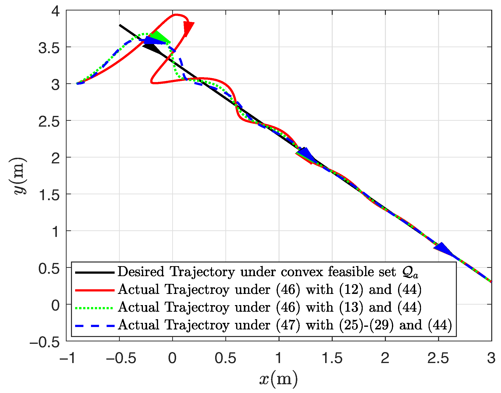
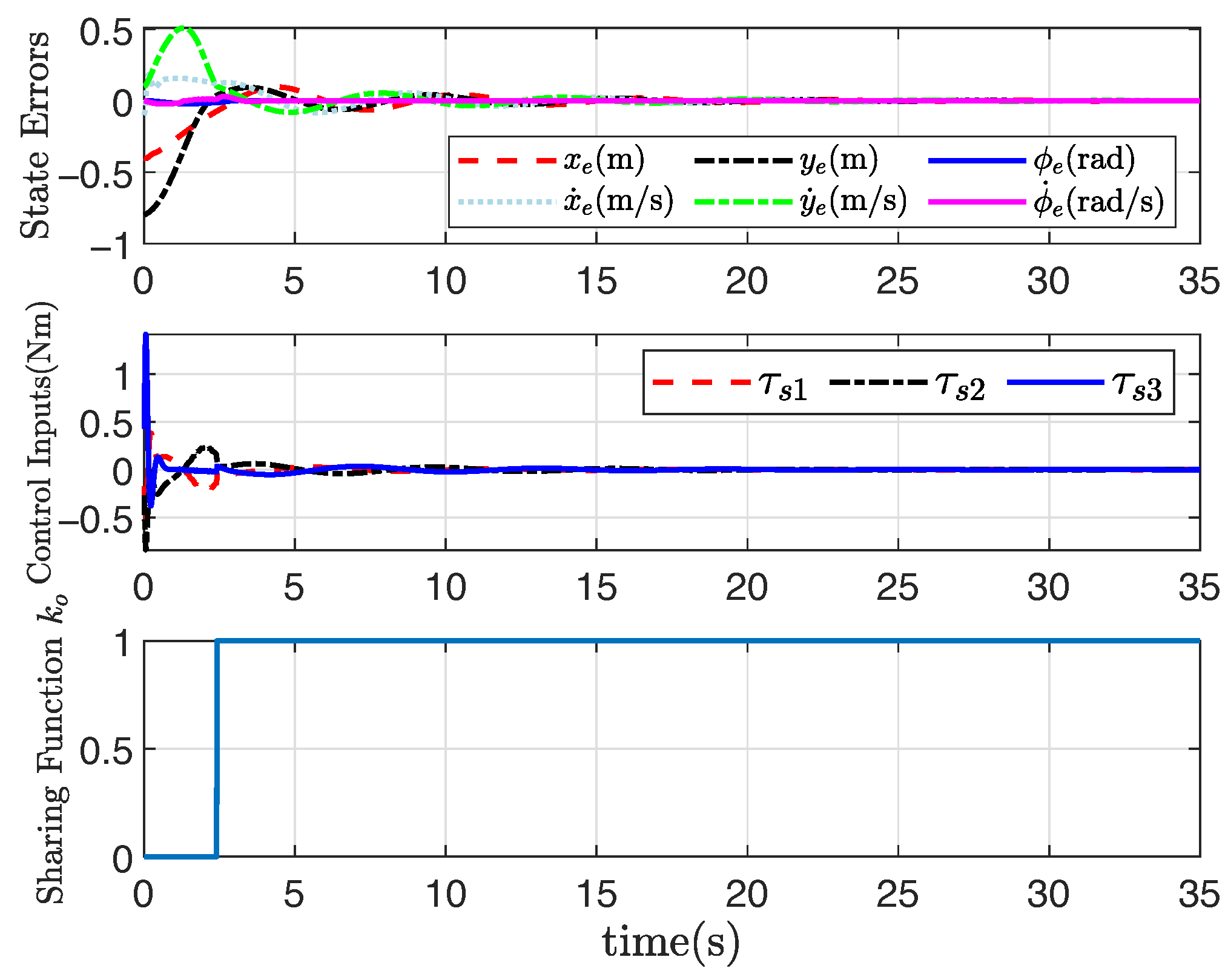
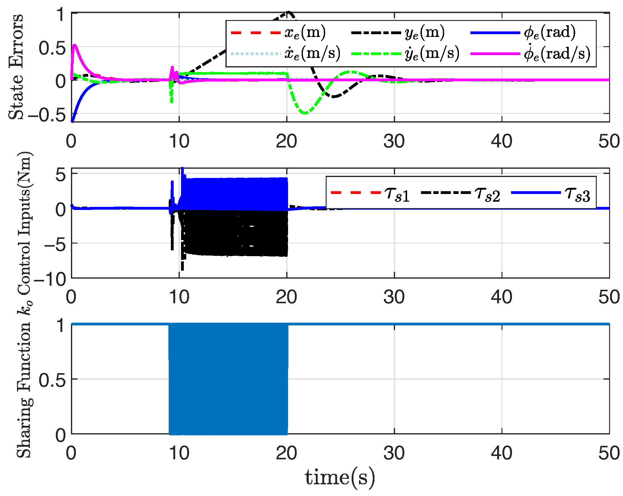
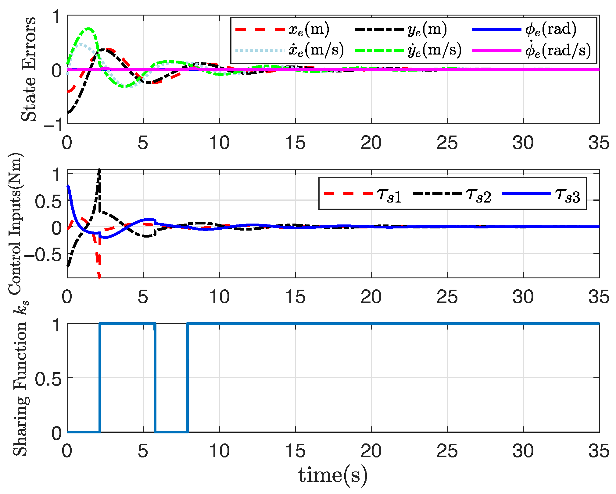
3.1. Machine Certainty-Equivalent Adaptive Control

Generally, the number of constraints on system outputs mainly depends on the control mission and the environment conditions. When $m>n$, only n constraints are activated according to (2), while when $m<n$, augment constraints $p_i<\alpha (i=1,2,\cdots ,n)$ with a sufficient large constant $\alpha$ can be added by the designer to the system until $m=n$. Without loss of generality, we devise the automatic controller for the scenario with $m=n$. The Euler–Lagrange system (1) with the coordinate ${\mathit{x}}^i$ is characterized by (3), and the corresponding automatic controller ${\mathit{u}}_f^i$ can be reformulated as

$$\left\{\begin{array}{c}{\dot{\mathit{x}}}^i=K^i{\dot{\mathit{q}}}^i=K^i{\mathit{v}}^i\hfill \\ M\left({\mathit{q}}^i\right){\dot{\mathit{v}}}^i+C({\mathit{q}}^i,{\mathit{v}}^i){\mathit{v}}^i+\mathit{g}\left({\mathit{q}}^i\right)={\mathit{u}}_f^i\hfill \\ {\mathit{x}}^i\le 0\hfill \end{array}\right.$$

(5)

where ${\mathit{q}}^i={\left(K^i\right)}^{-1}({\mathit{x}}^i-T^i)$. A new variable ${\mathit{z}}^i={[z_1^i,z_2^i,\cdots ,z_n^i]}^T$ is defined by

$$z_j^i=\ln {\displaystyle \frac{x_j^i}{x_{r_j}^i}},j\in \{1,2,\cdots ,n\},$$

(6)

to remove the constraint on ${\mathit{x}}^i$, where ${\mathit{x}}_r^i={[x_{r_1}^i,x_{r_2}^i,\cdots ,x_{r_n}^i]}^T$ is the reference signal for ${\mathit{x}}^i$ with $x_{r_j}^i$ defined by

$$x_{r_j}^i=\left\{\begin{array}{cc}-ϵ\hfill & m\ge -ϵ\hfill \\ -ϵ+m[1-{\mathrm{e}}^{\gamma (m+ϵ)}]\hfill & m<-ϵ\hfill \end{array}\right.,$$

(7)

and $m=s_j^i{p}_{d_j}+t_j^i$, $\gamma >0$, $ϵ>0$. It is noted that $x_{r_j}^i$ is the projected feasible reference that satisfies all constraints, i.e., $x_{r_j}^i<0$. Reference signal (7) is one possible smooth solution. In addition, according to (7), we also find that $x_{r_j}^i\approx m$ when m is sufficiently small, indicating that the reference signal tracks the human operator’s intentions as long as the human behavior is sufficiently safe (i.e., ${\mathit{q}}_d$ is far away from obstacles).

Since the smooth function $x_{r_j}^i<0$ for all $j\in \{1,2,\cdots ,n\}$, then ${\dot{\mathit{x}}}_r^i\left(t\right)$ and ${\ddot{\mathit{x}}}_r^i\left(t\right)$ exist and ${\mathit{q}}_r^i\left(t\right)={\left(K^i\right)}^{-1}({\mathit{x}}_r^i\left(t\right)-T^i)$, ${\mathit{v}}_r^i\left(t\right)={\left(K^i\right)}^{-1}{\dot{\mathit{x}}}_r^i\left(t\right)$, ${\dot{\mathit{v}}}_r^i\left(t\right)={\left(K^i\right)}^{-1}{\ddot{\mathit{x}}}_r^i\left(t\right)$. Furthermore, note that $({\mathit{q}}_r^i,{\mathit{v}}_r^i)\in {\mathcal{Q}}_a\times {\mathbb{R}}^n$.

Suppose $({\mathit{q}}_d,{\dot{\mathit{q}}}_d)$ denotes a point in ${\mathsf{\Lambda }}_h$ at $(\mathit{q},\dot{\mathit{q}})$ space, so the projection of $({\mathit{q}}_d,{\dot{\mathit{q}}}_d)$ into the safe subset ${\mathcal{O}}_s$ with regard to the ith set of motivation constraints, denoted by ${\mathsf{\Pi }}_{{\mathcal{O}}_s}^i({\mathit{q}}_d,{\dot{\mathit{q}}}_d)$, is characterized by ${\mathsf{\Pi }}_{{\mathcal{O}}_s}^i({\mathit{q}}_d,{\dot{\mathit{q}}}_d)=({\mathit{q}}_r^i,{\mathit{v}}_r^i)$. Thus, the projection of ${\mathsf{\Lambda }}_h$ into the subset ${\mathcal{O}}_s$ with regard to the ith group of active constraints is characterized as

$${\mathsf{\Pi }}_{{\mathcal{O}}_s}^i\left({\mathsf{\Lambda }}_h\right)=\{\phi \in {\mathcal{O}}_s|\phi ={\mathsf{\Pi }}_{{\mathcal{O}}_s}^i({\mathit{q}}_d,{\dot{\mathit{q}}}_d),\exists ({\mathit{q}}_d,{\dot{\mathit{q}}}_d)\in {\mathsf{\Lambda }}_h\}.$$

(8)

The velocity error is defined by ${\mathit{v}}_e^i={\mathit{v}}^i-{\mathit{v}}_r^i$ under the ith set of motivation constraints. Next, by differentiating ${\mathit{z}}^i$ and ${\mathit{v}}_e^i$, the tracking dynamics of the constrained Euler–Lagrange system is obtained by

$$\left\{\begin{array}{c}{\dot{\mathit{z}}}^i=Z_1{K}^i{\mathit{v}}_e^i+Z_2{K}^i{\mathit{v}}_r^i\hfill \\ M\left({\mathit{q}}^i\right){\dot{\mathit{v}}}_e^i+C({\mathit{q}}^i,{\mathit{v}}^i){\mathit{v}}_e^i+{\mathit{g}}_r^i={\mathit{u}}_f^i\hfill \end{array}\right.$$

(9)

where ${\mathit{g}}_r^i=M\left({\mathit{q}}^i\right){\dot{\mathit{v}}}_r^i+C({\mathit{q}}^i,{\mathit{v}}^i){\mathit{v}}_r^i+\mathit{g}\left({\mathit{q}}^i\right)$, $Z_1=\mathrm{diag}\left({\displaystyle \frac{{\mathrm{e}}^{-z_1^i}}{x_{r_1}^i}},{\displaystyle \frac{{\mathrm{e}}^{-z_2^i}}{x_{r_2}^i}},\cdots ,{\displaystyle \frac{{\mathrm{e}}^{-z_n^i}}{x_{r_n}^i}}\right),$ $Z_2=\mathrm{diag}\left({\displaystyle \frac{{\mathrm{e}}^{-z_1^i}-1}{x_{r_1}^i}},{\displaystyle \frac{{\mathrm{e}}^{-z_2^i}-1}{x_{r_2}^i}},\cdots ,{\displaystyle \frac{{\mathrm{e}}^{-z_n^i}-1}{x_{r_n}^i}}\right).$

In the backstepping control design framework, the virtual input of the first subsystem in (9) is formulated as $K^i{\mathit{v}}_e^{i★}={\mathit{z}}^i+Z_3{K}^i{\mathit{v}}_r^i$, where $Z_3=\mathrm{diag}({\mathrm{e}}^{z_1^i}-1,{\mathrm{e}}^{z_2^i}-1,\cdots ,{\mathrm{e}}^{z_n^i}-1)$. Then the virtual input derivative is $K^i{\dot{\mathit{v}}}_e^{i★}={\dot{\mathit{z}}}^i+{\dot{Z}}_3{K}^i{\mathit{v}}_r^i+Z_3{K}^i{\dot{\mathit{v}}}_r^i$. Furthermore, define ${\mathit{y}}^i={\mathit{v}}_e^i-{\mathit{v}}_e^{i★}$, and the tracking dynamics (9) is reformulated by

$$\left\{\begin{array}{c}{\dot{\mathit{z}}}^i=Z_1{K}^i{\mathit{y}}^i+Z_1{\mathit{z}}^i\hfill \\ M\left({\mathit{q}}^i\right){\dot{\mathit{y}}}^i+C({\mathit{q}}^i,{\mathit{v}}^i){\mathit{y}}^i+{\mathit{g}}_e^i={\mathit{u}}_f^i\hfill \end{array}\right.$$

(10)

where ${\mathit{g}}_e^i=M\left({\mathit{q}}^i\right){\dot{\mathit{v}}}_e^{i★}+C({\mathit{q}}^i,{\mathit{v}}^i){\mathit{v}}_e^{i★}+{\mathit{g}}_r^i$.

Define ${\mathit{p}}^i={\mathit{y}}^i-{\lambda }_q{\left(K^i\right)}^{-1}{\mathit{z}}^i$ with a tunable constant ${\lambda }_q>0$; then, the model (10) can be reformulated as

$$\left\{\begin{array}{c}{\dot{\mathit{z}}}^i=Z_1{K}^i{\mathit{p}}^i+({\lambda }_q+1)Z_1{\mathit{z}}^i\hfill \\ M\left({\mathit{q}}^i\right){\dot{\mathit{p}}}^i+C({\mathit{q}}^i,{\mathit{v}}^i){\mathit{p}}^i+Y^i\mathit{\theta }={\mathit{u}}_f^i\hfill \end{array}\right.$$

(11)

where $Y^i\mathit{\theta }=M\left({\mathit{q}}^i\right)[{\lambda }_q{\left(K^i\right)}^{-1}{\dot{\mathit{z}}}^i+{\dot{\mathit{v}}}_e^{i★}+{\dot{\mathit{v}}}_r^i]+C({\mathit{q}}^i,{\mathit{v}}^i)[{\lambda }_q{\left(K^i\right)}^{-1}{\mathit{z}}^i+{\mathit{v}}_e^{i★}+{\mathit{v}}_r^i]+\mathit{g}\left({\mathit{q}}^i\right)$, with the parametric vector $\mathit{\theta }\in {\mathbb{R}}^m$ formulated from the terms $M\left({\mathit{q}}^i\right)$, $C({\mathit{q}}^i$, ${\mathit{v}}^i)$, and $\mathit{g}\left({\mathit{q}}^i\right)$ and with the corresponding regression matrix $Y^i$ of $\mathit{\theta }$. Actually, this is the result of the linear parameterization property of model (1). Different sequences of parameters in the parameter vector result in different regression matrices. Thus, the explicit form of the known regressor $Y^i$ vs. the unknown parameter $\theta$ in (11) cannot be directly given based on the general model (1), unless the model (1) of the mechanical system is explicit.

Design the certainty-equivalent adaptive state feedback controller as

$${\mathit{u}}_f^i=-K{\mathit{p}}^i-{K^i}^T{Z}_1^T{\mathit{z}}^i+Y^i\hat{\mathit{\theta }},\dot{\hat{\mathit{\theta }}}=-{\displaystyle \frac{1}{{\gamma }_{\theta }}}{Y^i}^T{\mathit{p}}^i,$$

(12)

where K is a positive-definite matrix; $\hat{\mathit{\theta }}$ is the estimation of $\mathit{\theta }$; and ${\gamma }_{\theta }>0$ is a tunable constant.

Theorem 1. 

For the nonlinear constrained system (1) under Assumptions 1 and 2, if the state-feedback adaptive control law is designed by (12), then it can be readily demonstrated such that the controlled system satisfies ${\mathit{q}}^i\to {\mathit{q}}_r^i$ and ${\mathit{v}}^i\to {\mathit{v}}_r^i$ as $t\to \infty$.

Proof. 

Choose a candidate Lyapunov function for the system (11) by $L^i={\displaystyle \frac{1}{2}}[{{\mathit{z}}^i}^T{\mathit{z}}^i+{{\mathit{p}}^i}^{T}M\left({\mathit{q}}^i\right){\mathit{p}}^i+{\gamma }_{\theta }{\tilde{\mathit{\theta }}}^T\tilde{\mathit{\theta }}]\ge 0$ with parametric estimation error $\tilde{\mathit{\theta }}=\widehat{\mathit{\theta }}-\mathit{\theta }$. Then, the derivative of $L^i$ along the trajectory of (11) with controller (12) satisfies ${\dot{L}}^i=({\lambda }_q+1){{\mathit{z}}^i}^T{Z}_1{\mathit{z}}^i-{{\mathit{p}}^i}^{T}K{\mathit{p}}^i$. Since $Z_1$ and K are negative definite and positive definite matrices, then ${\dot{L}}^i\le 0$, which indicates that both ${\mathit{z}}^i$ and ${\mathit{p}}^i$ are bounded. In addition, the second derivative with respect to $L^i$ is given as ${\ddot{L}}^i=({\lambda }_q+1)(2{{\mathit{z}}^i}^T{Z}_1{\dot{\mathit{z}}}^i+{{\mathit{z}}^i}^T{\dot{Z}}_1{\mathit{z}}^i)-{\left({\dot{\mathit{p}}}^i\right)}^{T}K{\mathit{p}}^i-{{\mathit{p}}^i}^{T}K{\dot{\mathit{p}}}^i$. According to the definition of ${\mathit{p}}^i$ and (10), it can be concluded that both ${\dot{\mathit{p}}}^i$ and ${\dot{\mathit{z}}}^i$ exist and are bounded; therefore, ${\ddot{L}}^i$ exists and is bounded. From Barbalat’s Lemma [13], it is immediately concluded that ${\mathit{z}}^i\to 0$ and ${\mathit{p}}^i\to 0$ as $t\to \infty$. Furthermore, it can be concluded that ${\mathit{q}}^i\to {\mathit{q}}_r^i$ and ${\mathit{v}}^i\to {\mathit{v}}_r^i$ as $t\to \infty$. □

Remark 2. 

The concept of certainty equivalence in traditional adaptive control is an important feature. This implies that initially, a controller is constructed under the assumption that all the system parameters are known. Controller parameters are defined by a function of all model parameters. Given the actual values of the model parameters, the controller parameters of the controller are computed by solving design equations aimed at pole-zero placement, model matching, or optimality. When actual model parameters are unavailable, controller parameters can be either estimated directly or computed indirectly by solving the identical design equations utilizing estimations of the model parameters. The obtained controller, which is estimated or designed specifically for the estimated model, is termed a certainty equivalence adaptive controller. However, since certainty-equivalent adaptive law is generally just an integrator about system states, the parameter estimator performance depends on the state tracking performance.

3.2. Machine Non-Certainty-Equivalent Adaptive Control

Based on (11), one can design non-certainty-equivalent adaptive control law as

$$\left\{\begin{array}{c}{\mathit{u}}_f^i=-W^i(\widehat{\mathit{\theta }}+\mathit{\beta })-{\gamma }_n{W}_n^i{W_n^i}^T[{\mathit{p}}^i+(k_q-{\alpha }_n){\mathit{p}}_n^i]\hfill \\ \dot{\widehat{\mathit{\theta }}}={\gamma }_n{({\alpha }_n{W}_n^i-W^i)}^T{\mathit{p}}_n^i+{\gamma }_n{k}_q{W_n^i}^T{\mathit{p}}_n^i\hfill \end{array}\right.$$

(13)

with $\mathit{\beta }={\gamma }_n{W_n^i}^T{\mathit{p}}_n^i$, the stable first-order linear filters

$${\dot{\mathit{p}}}_n^i=-{\alpha }_n{\mathit{p}}_n^i+{\mathit{p}}^i,{\dot{W}}_n^i=-{\alpha }_n{W}_n^i+W^i,$$

(14)

and the regression matrix $W^i$ defined by $W^i\mathit{\theta }=\dot{M}\left({\mathit{q}}^i\right)[{\mathit{p}}^i+(k_q-{\alpha }_n){\mathit{p}}_n^i]+k_{q}M\left({\mathit{q}}^i\right){\mathit{p}}^i-C({\mathit{q}}^i,{\mathit{v}}^i){\mathit{p}}^i-Y^i\mathit{\theta }$, where ${\alpha }_n>0$, $k_q>0$, and ${\gamma }_n\ge {\displaystyle \frac{1}{k_q}}$.

Theorem 2. 

For the nonlinear constrained system (1) under Assumptions 1 and 2, if the machine adaptive controller is designed by (13) and (14) with conditions

$${\mathit{p}}_n^i\left(0\right)={\displaystyle \frac{{\mathit{p}}^i\left(0\right)}{{\alpha }_n-k_q}},{\alpha }_n-k_q\ne 0,W_n^i\left(0\right)=\mathbf{0}.$$

(15)

then it is also readily demonstrated from [14,15] that the closed-loop system satisfies ${\mathit{q}}^i\to {\mathit{q}}_r^i$ and ${\mathit{v}}^i\to {\mathit{v}}_r^i$ as $t\to \infty$.

Proof. 

Adding and subtracting $\dot{M}\left({\mathit{q}}^i\right)[{\mathit{p}}^i+(k_q-{\alpha }_n){\mathit{p}}_n^i]+k_{q}M\left({\mathit{q}}^i\right){\mathit{p}}^i$ into the right-hand side of dynamics $M\left({\mathit{q}}^i\right){\dot{\mathit{p}}}^i+C({\mathit{q}}^i,{\mathit{v}}^i){\mathit{p}}^i+Y^i\mathit{\theta }={\mathit{u}}_f^i$ in (11) results in

$$M\left({\mathit{q}}^i\right){\dot{\mathit{p}}}^i=W^i\mathit{\theta }+{\mathit{u}}_f^i-\dot{M}\left({\mathit{q}}^i\right)[{\mathit{p}}^i+(k_q-{\alpha }_n){\mathit{p}}_n^i]-k_{q}M\left({\mathit{q}}^i\right){\mathit{p}}^i$$

(16)

Denote a linear filter for the control signal as

$${\dot{\mathit{u}}}_n^i=-{\alpha }_n{\mathit{u}}_n^i+{\mathit{u}}_f^i,{\mathit{u}}_n^i\left(0\right)=\mathbf{0}.$$

(17)

Then substitute (14) and (17) into (16) to yield the filtered-state error dynamics

$$\begin{array}{cc}\hfill & {\displaystyle \frac{\mathrm{d}}{\mathrm{d}t}}[M\left({\mathit{q}}^i\right)({\dot{\mathit{p}}}_n^i+k_q{\mathit{p}}_n^i)-W_n^i\mathit{\theta }-{\mathit{u}}_n^i]\hfill \\ \hfill & =-{\alpha }_n[M\left({\mathit{q}}^i\right)({\dot{\mathit{p}}}_n^i+k_q{\mathit{p}}_n^i)-W_n^i\mathit{\theta }-{\mathit{u}}_n^i].\hfill \end{array}$$

(18)

Thus, the solution of system (18) can be immediately derived by ${\dot{\mathit{p}}}_n^i=-k_q{\mathit{p}}_n^i+M^{-1}\left({\mathit{q}}^i\right)(W_n^i\mathit{\theta }+{\mathit{u}}_n^i)+M^{-1}\left({\mathit{q}}^i\right)\mathit{\zeta }\left(t\right)$, where $\mathit{\zeta }\left(t\right)=[M\left({\mathit{q}}^i\left(0\right)\right)({\dot{\mathit{p}}}_n^i\left(0\right)+k_q{\mathit{p}}_n^i\left(0\right))-W_n^i\left(0\right)\mathit{\theta }-{\mathit{u}}_n^i\left(0\right)]{\mathrm{e}}^{-{\alpha }_{n}t}$. It can be seen that $\mathit{\zeta }\left(t\right)$ is an exponentially decaying term and its initial value directly depends on ${\mathit{q}}^i\left(0\right)$, ${\dot{\mathit{p}}}_n^i\left(0\right)$, ${\mathit{p}}_n^i\left(0\right)$, $W_n^i\left(0\right)$, and ${\mathit{u}}_n^i\left(0\right)$. Thus $\mathit{\zeta }\left(t\right)\equiv \mathbf{0}$ for all $t\ge 0$ is equivalent to following conditions about tunable parameters: ${\dot{\mathit{p}}}_n^i\left(0\right)+k_q{\mathit{p}}_n^i\left(0\right)=\mathbf{0}$, $W_n^i\left(0\right)=\mathbf{0}$, and ${\mathit{u}}_n^i\left(0\right)=\mathbf{0}$. Furthermore, based on (14), this means that initial values of filters should satisfy (15).

Thus, $\mathit{\zeta }\left(t\right)\equiv \mathbf{0}$ leads to the filtered-state error dynamics as

$${\dot{\mathit{p}}}_n^i=-k_q{\mathit{p}}_n^i+M^{-1}\left({\mathit{q}}^i\right)(W_n^i\mathit{\theta }+{\mathit{u}}_n^i).$$

(19)

Define the parameter estimation error $\tilde{\mathit{\theta }}=\widehat{\mathit{\theta }}+\mathit{\beta }-\mathit{\theta }$ and the filtered control signal ${\mathit{u}}_n^i=-W_n^i(\widehat{\mathit{\theta }}+\mathit{\beta })$; then, the filtered-state error dynamics (19) can be rewritten as

$${\dot{\mathit{p}}}_n^i=-k_q{\mathit{p}}_n^i-M^{-1}\left({\mathit{q}}^i\right)W_n^i\tilde{\mathit{\theta }},$$

(20)

and the derivation of the dynamics of the estimation error is obtained by

$$\dot{\tilde{\mathit{\theta }}}=\dot{\widehat{\mathit{\theta }}}+\dot{\mathit{\beta }}=-{\gamma }_n{W_n^i}^T{M}^{-1}\left({\mathit{q}}^i\right)W_n^i\tilde{\mathit{\theta }}.$$

(21)

Set a candidate Lyapunov function for (11) by $L^i={\displaystyle \frac{1}{2}}{{\mathit{p}}_n^i}^T{\mathit{p}}_n^i+{\displaystyle \frac{1}{2\underline{m}}}{\tilde{\mathit{\theta }}}^T\tilde{\mathit{\theta }}\ge 0$. Then, recalling ${\gamma }_n\ge {\displaystyle \frac{1}{k_q}}$ and taking the time derivative of $L^i$ along the trajectory of (20) and (21) yields

$$\begin{array}{cc}\hfill {\dot{L}}^i=& {{\mathit{p}}_n^i}^T[-k_q{\mathit{p}}_n^i-M^{-1}\left({\mathit{q}}^i\right)W_n^i\tilde{\mathit{\theta }}]+{\displaystyle \frac{1}{\underline{m}}}{\tilde{\mathit{\theta }}}^T(\dot{\widehat{\mathit{\theta }}}+\dot{\mathit{\beta }})\hfill \\ \hfill =& -k_q{{\mathit{p}}_n^i}^T{\mathit{p}}_n^i-{{\mathit{p}}_n^i}^T{M}^{-1}\left({\mathit{q}}^i\right)W_n^i\tilde{\mathit{\theta }}\hfill \\ \hfill & -{\displaystyle \frac{{\gamma }_n}{\underline{m}}}{\tilde{\mathit{\theta }}}^T{W_n^i}^T{M}^{-1}\left({\mathit{q}}^i\right)W_n^i\tilde{\mathit{\theta }}\hfill \\ \hfill \le & -{\displaystyle \frac{k_q}{2}}\parallel {\mathit{p}}_n^i{\parallel }^2-{\displaystyle \frac{{\gamma }_n}{2}}{\parallel M^{-1}\left({\mathit{q}}^i\right)W_n^i\tilde{\mathit{\theta }}\parallel }^2\le 0.\hfill \end{array}$$

(22)

Thus, it can be concluded from Barbalat’s Lemma [13] that ${\mathit{p}}_n^i\to \mathbf{0}$ and $\left[M^{-1}\left({\mathit{q}}^i\right)W_n^i\tilde{\mathit{\theta }}\right]\to \mathbf{0}$ as $t\to \infty$. Then, based on the stability of the linear filters in (14), it can be concluded that ${\mathit{p}}^i\to \mathbf{0}$ as $t\to \infty$. Furthermore, since $Z_1$ is a negative definite matrix in (11) and ${\mathit{p}}^i\to \mathbf{0}$ as $t\to \infty$, it is immediately concluded that ${\mathit{z}}^i\to \mathbf{0}$ and ${\mathit{y}}^i\to \mathbf{0}$ as $t\to \infty$. Therefore, ${\mathit{q}}^i\to {\mathit{q}}_r^i$ and ${\mathit{v}}^i\to {\mathit{v}}_r^i$ as $t\to \infty$.

Finally, the adaptive state-feedback control input ${\mathit{u}}_f^i$ can be retrieved from the filtered control signal ${\mathit{u}}_n^i$ in (17) and ${\mathit{u}}_n^i=-W_n^i(\widehat{\mathit{\theta }}+\mathit{\beta })$ as ${\mathit{u}}_f^i={\dot{\mathit{u}}}_n^i+{\alpha }_n{\mathit{u}}_n^i=-W^i(\widehat{\mathit{\theta }}+\mathit{\beta })-W_n^i(\dot{\widehat{\mathit{\theta }}}+\dot{\mathit{\beta }})=-W^i(\widehat{\mathit{\theta }}+\mathit{\beta })-{\gamma }_n{W}_n^i{W_n^i}^T[{\mathit{p}}^i+(k_q-{\alpha }_n){\mathit{p}}_n^i]$, which is the same as (13), thus concluding the verification. □

Remark 3. 

Founded on the non-certainty-equivalent principle, the adaptive law of plant parameters could be designed as a stable filter, and the estimator performance could also be improved with the tunable parameter in the filter. Moreover, the estimate parameters of the non-certainty-equivalent adaptive system encompasses not only the estimates from the adaptive dynamic subsystem but also nonlinear functions. The inclusion of additional nonlinear functions within the estimated parameter vector enhances the performance of the controller. A typical non-certainty-equivalent adaptive design technique is the immersion and invariance manifold method. This method aims to keep the manifold’s invariable and attractive properties such that the overall system is stable. This idea is also applied to the adaptive estimator. If the error between the estimation of the plant parameter and its true value is chosen as the invariable manifold and the suitable nonlinear function in the adaptive law is designed, then the estimation error could be always bounded by small constants even asymptotically converging to zero. Thus, the non-certainty-equivalent adaptive controller generally has better parameter estimation capability than the traditional certainty-equivalent adaptive controller. Moreover, since the considered nonlinear mechanical system has the double-integrator structure and the model linear parametrization property, the certainty-equivalent and non-certainty-equivalent principles could be easily employed in the feedback control subsystem designed in this study.

3.3. Machine Adaptive Output-Feedback Control

The error Equation (9) can be reformulated as

$$M\left({\mathit{q}}^i\right){\left(K^i\right)}^{-1}{Z}_1^{-1}{\ddot{\mathit{z}}}^i+{\mathit{f}}_a+{\mathit{f}}_b={\mathit{u}}_f^i,$$

(23)

where ${\mathit{f}}_a=M\left({\mathit{q}}^i\right)Z_1^{-1}{\dot{Z}}_1[Z_1^{-1}{Z}_2{\mathit{v}}_r^i-{\left(K^i\right)}^{-1}{Z}_1^{-1}{\dot{\mathit{z}}}^i]+C({\mathit{q}}^i,{\left(K^i\right)}^{-1}{Z}_1^{-1}{\dot{\mathit{z}}}^i)[{\left(K^i\right)}^{-1}{Z}_1^{-1}{\dot{\mathit{z}}}^i+2{\mathit{v}}_r^i-2Z_1^{-1}{Z}_2{\mathit{v}}_r^i]-M\left({\mathit{q}}^i\right)Z_1^{-1}{\dot{Z}}_2{\mathit{v}}_r^i$, ${\mathit{f}}_b=M\left({\mathit{q}}^i\right)[{\dot{\mathit{v}}}_r^i-Z_1^{-1}{Z}_2{\dot{\mathit{v}}}_r^i]+C({\mathit{q}}^i,{\mathit{v}}_r^i-Z_1^{-1}{Z}_2{\mathit{v}}_r^i)({\mathit{v}}_r^i-Z_1^{-1}{Z}_2{\mathit{v}}_r^i)+\mathit{g}\left({\mathit{q}}^i\right)$. Clearly, since ${\mathit{f}}_b$ can be written as ${\mathit{f}}_b={\mathsf{\Psi }}^i\mathit{\theta }$ based on the linear parametrization, then the model (23) can be parameterized as

$$M\left({\mathit{q}}^i\right){\left(K^i\right)}^{-1}{Z}_1^{-1}{\ddot{\mathit{z}}}^i+{\mathit{f}}_a+{\mathsf{\Psi }}^i\mathit{\theta }={\mathit{u}}_f^i,$$

(24)

Furthermore, it can be seen that $M\left({\mathit{q}}^i\right){\left(K^i\right)}^{-1}{Z}_1^{-1}$ and ${\mathit{f}}_a$ are the first-order continuously differentiable functions.

The adaptive output feedback control law for (23) is proposed as

$${\mathit{u}}_f^i=-{\left(K^i\right)}^T{Z}_1^T[K_1\mathrm{sgn}({\mathit{z}}^i+{\mathit{z}}_f^i)-(k_2+1){\mathit{r}}_f^i+{\mathit{z}}^i]-{\mathsf{\Psi }}^i\widehat{\mathit{\theta }},$$

(25)

$${\dot{\mathit{z}}}_f^i=-{\mathit{z}}_f^i+{\mathit{r}}_f^i,{\mathit{z}}_f^i\left(0\right)=\mathbf{0},$$

(26)

$${\mathit{r}}_f^i={\mathit{\xi }}^i-(k_2+1){\mathit{z}}^i,$$

(27)

$$\left\{\begin{array}{c}{\dot{\mathit{\xi }}}^i=-{\mathit{r}}_f^i-(k_2+1)({\mathit{z}}^i+{\mathit{r}}_f^i)+{\mathit{z}}^i-{\mathit{z}}_f^i,\hfill \\ {\mathit{\xi }}^i\left(0\right)=(k_2+1){\mathit{z}}^i\left(0\right),\hfill \end{array}\right.$$

(28)

$$\dot{\widehat{\mathit{\theta }}}={\displaystyle \frac{1}{{\gamma }_{\theta }}}{\left(K^i\right)}^{-T}{Z}_1^{-T}{\left({\mathsf{\Psi }}^i\right)}^T({\mathit{z}}^i+{\mathit{r}}_f^i),$$

(29)

where ${\mathit{z}}_f^i$ and ${\mathit{r}}_f^i$ are filtered signals; $\widehat{\mathit{\theta }}$ is the estimation of $\mathit{\theta }$; ${\mathit{\xi }}^i$ is an auxiliary variable used in the filter; $K_1$ is a constant, diagonal, positive-definite matrix; $k_2$ is a positive constant; and $\mathrm{sgn}\left(\mathit{a}\right)={[\mathrm{sgn}\left(a_1\right),\mathrm{sgn}\left(a_2\right),\cdots ,\mathrm{sgn}\left(a_n\right)]}^T$ for any $\mathit{a}\in {\mathbb{R}}^n$ with $\mathrm{sgn}(·)$ being the standard signum function.

To facilitate the stability analysis of the controlled system, define a signal as

$${\mathit{\eta }}^i={\dot{\mathit{z}}}^i+{\mathit{z}}^i+{\mathit{r}}_f^i,$$

(30)

Then, taking the time derivative of ${\mathit{r}}_f^i$ in (27) with a signal in (30) leads to

$${\dot{\mathit{r}}}_f^i=-{\mathit{r}}_f^i-(k_2+1){\mathit{\eta }}^i+{\mathit{z}}^i-{\mathit{z}}_f^i.$$

(31)

Taking the time derivative of ${\mathit{\eta }}^i$ in (30) yields

$${\dot{\mathit{\eta }}}^i={\ddot{\mathit{z}}}^i-{\mathit{z}}_f^i-2{\mathit{r}}_f^i-k_2{\mathit{\eta }}^i.$$

(32)

After multiplying (32) by $Z_1^{-T}{\left(K^i\right)}^{-T}M\left({\mathit{q}}^i\right){\left(K^i\right)}^{-1}{Z}_1^{-1}$ and substituting (25) into (24), the closed-loop system is

$$\begin{array}{cc}\hfill & Z_1^{-T}{\left(K^i\right)}^{-T}M\left({\mathit{q}}^i\right){\left(K^i\right)}^{-1}{Z}_1^{-1}{\dot{\mathit{\eta }}}^i=-k_2{Z}_1^{-T}{\left(K^i\right)}^{-T}M\left({\mathit{q}}^i\right){\left(K^i\right)}^{-1}{Z}_1^{-1}{\mathit{\eta }}^i\hfill \\ \hfill & -{\displaystyle \frac{1}{2}}{Z}_1^{-T}{\left(K^i\right)}^{-T}\dot{M}\left({\mathit{q}}^i\right){\left(K^i\right)}^{-1}{Z}_1^{-1}{\mathit{\eta }}^i-Z_1^{-T}{\left(K^i\right)}^{-T}M\left({\mathit{q}}^i\right){\left(K^i\right)}^{-1}{\dot{Z}}_1^{-1}{\mathit{\eta }}^i\hfill \\ \hfill & +\tilde{\mathit{f}}-K_1\mathrm{sgn}({\mathit{z}}^i+{\mathit{z}}_f^i)+(k_2+1){\mathit{r}}_f^i-{\mathit{z}}^i-Z_1^{-T}{\left(K^i\right)}^{-T}{\mathsf{\Psi }}^i\tilde{\mathit{\theta }},\hfill \end{array}$$

(33)

where $\tilde{\mathit{f}}=-Z_1^{-T}{\left(K^i\right)}^{-T}[{\mathit{f}}_a+M\left({\mathit{q}}^i\right){\left(K^i\right)}^{-1}{Z}_1^{-1}({\mathit{z}}_f^i+2{\mathit{r}}_f^i)-{\displaystyle \frac{1}{2}}\dot{M}\left({\mathit{q}}^i\right){\left(K^i\right)}^{-1}{Z}_1^{-1}{\mathit{\eta }}^i-M\left({\mathit{q}}^i\right){\left(K^i\right)}^{-1}{\dot{Z}}_1^{-1}{\mathit{\eta }}^i]$ and the parameter estimation error is $\tilde{\mathit{\theta }}=\widehat{\mathit{\theta }}-\mathit{\theta }$.

Remark 4. 

Since ${\mathit{f}}_a$ defined in (23) is continuously differentiable, it is shown that $\tilde{\mathit{f}}$ in (33) is upper-bounded by $\parallel \tilde{\mathit{f}}\parallel \le \varphi (\parallel {\mathit{\varphi }}^i\parallel )\parallel {\mathit{\varphi }}^i\parallel$ with ${\mathit{\varphi }}^i\triangleq {[{\left({\mathit{z}}^i\right)}^T,{\left({\mathit{z}}_f^i\right)}^T,{\left({\mathit{r}}_f^i\right)}^T,{\left({\mathit{\eta }}^i\right)}^T]}^T$, and the positive function $\varphi (\parallel {\mathit{\varphi }}^i\parallel )$ is non-decreasing in $\parallel {\mathit{\varphi }}^i\parallel$.

Lemma 1. 

Define a function $l\left(t\right)=-{\left({\mathit{\eta }}^i\right)}^T{K}_1\mathit{sgn}({\mathit{z}}^i+{\mathit{z}}_f^i)$. If the control gain matrix $K_1$ is selected to satisfy the sufficient condition $k_{1j}>0$, where $k_{1j}$ is the jth entry of the diagonal matrix $K_1$, then it can be derived that ${\int }_0^{t}l\left(\tau \right)d\tau \le {\overline{l}}_b$ with the positive constant ${\overline{l}}_b\triangleq {\sum }_{j=1}^n{k}_{1j}\left|z_j^i\left(0\right)\right|$.

Proof. 

From (26) and (30), one has ${\mathit{\eta }}^i=({\dot{\mathit{z}}}^i+{\dot{\mathit{z}}}_f^i)+({\mathit{z}}^i+{\mathit{z}}_f^i)$ with ${\mathit{z}}_f^i\left(0\right)=\mathbf{0}$. Then ${\int }_0^{t}l\left(\tau \right)\mathrm{d}\tau \le -{\int }_0^t{\displaystyle \frac{\mathrm{d}{({\mathit{z}}^i+{\mathit{z}}_f^i)}^T}{\mathrm{d}\tau }}{K}_1\mathrm{sgn}({\mathit{z}}^i+{\mathit{z}}_f^i)\mathrm{d}\tau =-{\left.{\sum }_{j=1}^n{k}_{1j}|z_j^i\left(\tau \right)+z_{f_j}^i\left(\tau \right)|\right|}_0^t\le {\overline{l}}_b$. □

Theorem 3. 

Consider the output-constrained system (1) under Assumptions 1–2. If the adaptive output-feedback controller is designed by (25), then the closed-loop system signals are bounded and ${\mathit{q}}^i\to {\mathit{q}}_r^i$ and ${\mathit{v}}^i\to {\mathit{v}}_r^i$ as $t\to \infty$, where $K_1$ is chosen to satisfy $k_{1i}>0$, and $k_2={\displaystyle \frac{k_n+1}{\underline{m}}}$ with constant $k_n>0$.

Proof. 

Define a function $l_c\triangleq {\overline{l}}_b-{\int }_0^{t}l\left(\tau \right)\mathrm{d}\tau \ge 0$ from Lemma 1. Choose a function as

$$\begin{array}{cc}\hfill L^i=& {\displaystyle \frac{1}{2}}[{\left({\mathit{z}}^i\right)}^T{\mathit{z}}^i+{\left({\mathit{z}}_f^i\right)}^T{\mathit{z}}_f^i+{\left({\mathit{r}}_f^i\right)}^T{\mathit{r}}_f^i+{\gamma }_{\theta }{\tilde{\mathit{\theta }}}^T\tilde{\mathit{\theta }}+2l_c\hfill \\ \hfill & +{\left({\left(K^i\right)}^{-1}{Z}_1^{-1}{\mathit{\eta }}^i\right)}^{T}M\left({\mathit{q}}^i\right){\left(K^i\right)}^{-1}{Z}_1^{-1}{\mathit{\eta }}^i]\ge 0.\hfill \end{array}$$

(34)

Note that (34) can be bounded by

$${\sigma }_a\left({\mathit{z}}^i\right){\parallel \mathit{\delta }\parallel }^2\le L^i\le {\sigma }_b\left({\mathit{z}}^i\right){\parallel \mathit{\delta }\parallel }^2,$$

(35)

where $\mathit{\delta }={[{\left({\mathit{\varphi }}^i\right)}^T,{\tilde{\mathit{\theta }}}^T,\sqrt{l_c}]}^T$, ${\sigma }_a\left({\mathit{z}}^i\right)\triangleq {\displaystyle \frac{1}{2}}\min \{1,{\gamma }_{\theta },\underline{m}\parallel {\left(K^i\right)}^{-1}{Z}_1^{-1}{\parallel }^2\}$ and ${\sigma }_b\left({\mathit{z}}^i\right)\triangleq \max \{1,{\displaystyle \frac{1}{2}}{\gamma }_{\theta },{\displaystyle \frac{1}{2}}\overline{m}\parallel {\left(K^i\right)}^{-1}{Z}_1^{-1}{\parallel }^2\}$. The time derivative of $L^i$ along the system trajectory of (33) is given by

$$\begin{array}{cc}\hfill {\dot{L}}^i\le & -{\left({\mathit{z}}^i\right)}^T{\mathit{z}}^i-{\left({\mathit{z}}_f^i\right)}^T{\mathit{z}}_f^i-{\left({\mathit{r}}_f^i\right)}^T{\mathit{r}}_f^i+{\mathit{f}}_c\hfill \\ \hfill & -k_2{\left({\mathit{\eta }}^i\right)}^T{Z}_1^{-T}{\left(K^i\right)}^{-T}M\left({\mathit{q}}^i\right){\left(K^i\right)}^{-1}{Z}_1^{-1}{\mathit{\eta }}^i\hfill \\ \hfill \le & -\parallel {\mathit{\varphi }}^i{\parallel }^2+[\parallel {\mathit{\eta }}^i\parallel \varphi (\parallel {\mathit{\varphi }}^i\parallel )\parallel {\mathit{\varphi }}^i\parallel -k_n\parallel {\mathit{\eta }}^i{\parallel }^2]\hfill \\ \hfill \le & -\left(1-{\displaystyle \frac{{\varphi }^2(\parallel {\mathit{\varphi }}^i\parallel )}{4k_n}}\right){\parallel {\mathit{\varphi }}^i\parallel }^2,\hfill \end{array}$$

(36)

where ${\mathit{f}}_c={\left({\mathit{\eta }}^i\right)}^T\tilde{\mathit{f}}-{\left({\dot{\mathit{z}}}^i\right)}^T{Z}_1^{-T}{\left(K^i\right)}^{-T}{\mathsf{\Psi }}^i\tilde{\mathit{\theta }}$, $\parallel {\mathit{f}}_c\parallel \le \parallel {\mathit{\eta }}^i\parallel \varphi (\parallel {\mathit{\varphi }}^i\parallel )\parallel {\mathit{\varphi }}^i\parallel ,$ $k_n\ge {\displaystyle \frac{1}{4}}{\varphi }^2\left(\sqrt{{\displaystyle \frac{{\sigma }_b\left({\mathit{z}}^i\left(0\right)\right)}{{\sigma }_a\left({\mathit{z}}^i\left(0\right)\right)}}}\parallel \mathit{\delta }\left(0\right)\parallel \right)$, and $\parallel \mathit{\delta }\left(0\right)\parallel =\sqrt{\parallel {\mathit{z}}^i{\left(0\right)\parallel }^2+\parallel {\mathit{\eta }}^i{\left(0\right)\parallel }^2+{\sum }_{j=1}^n{k}_{1j}\left|z_j^i\left(0\right)\right|}$. This means that

$${\dot{L}}^i\le -\varpi {\parallel {\mathit{\varphi }}^i\parallel }^2$$

(37)

for $k_n>{\displaystyle \frac{1}{4}}{\varphi }^2(\parallel {\mathit{\varphi }}^i\parallel )$ or $\parallel {\mathit{\varphi }}^i\parallel <{\varphi }^{-1}\left(2\sqrt{k_n}\right)$, where $\varpi$ is a positive constant. Then, following Theorem 8.4 in [13], one can define the region as $\mathsf{\Lambda }\triangleq \{\mathit{\delta }\in {\mathbb{R}}^{4n}\times {\mathbb{R}}^m\times {\mathbb{R}}_{+}|\parallel \mathit{\delta }\parallel <{\varphi }^{-1}\left(2\sqrt{k_n}\right)\}$. From (35) and (37), we know that ${\mathit{z}}^i$, ${\mathit{z}}_f^i$, ${\mathit{r}}_f^i$, ${\mathit{\eta }}^i$, and $\widehat{\mathit{\theta }}$ are bounded. From (30), we further know that ${\dot{\mathit{z}}}^i$ is also bounded. Then, from (26)–(28), we know that ${\dot{\mathit{z}}}_f^i$, ${\mathit{\xi }}^i$, and ${\dot{\mathit{\xi }}}^i$ are bounded. Furthermore, since ${\mathit{f}}_a$ is a first-order continuously differentiable function, then it is also a bounded function. Then, from (25) and (23), we know that the feedback control inputs ${\mathit{u}}_f^i$ and ${\ddot{\mathit{z}}}^i$ are bounded. Based on the above boundedness statements, it can be deduced that ${\dot{W}}_c\left(\mathit{\delta }\right)$ is also bounded, which is a sufficient condition for $W_c\left(\mathit{\delta }\right)=\varpi {\parallel {\mathit{\varphi }}^i\parallel }^2$ being uniformly continuous. If we define the region ${\mathsf{\Lambda }}_0\triangleq \{\mathit{\delta }\in \mathsf{\Lambda }|W_b\left(\mathit{\delta }\right)<{\sigma }_a\left({\mathit{z}}^i\left(0\right)\right){\left({\varphi }^{-1}\left(2\sqrt{k_n}\right)\right)}^2\}$, then we can recall Theorem 8.4 in [13] to state that $\varpi \parallel {\mathit{\varphi }}^i{\parallel }^2\to 0$ as $t\to \infty$ for any $\mathit{\delta }\left(0\right)\in {\mathsf{\Lambda }}_0$. Then, from the definition of ${\mathit{\varphi }}^i$ in Remark 1, we know ${\mathit{z}}^i\to \mathbf{0}$, ${\mathit{z}}_f^i\to \mathbf{0}$, ${\mathit{r}}_f^i\to \mathbf{0}$, and ${\mathit{\eta }}^i\to \mathbf{0}$ as $t\to \infty$ for any $\mathit{\delta }\left(0\right)\in {\mathsf{\Lambda }}_0$. Furthermore, it can be concluded from (30) that ${\dot{\mathit{z}}}^i\to \mathbf{0}$ as $t\to \infty$ for any $\mathit{\delta }\left(0\right)\in {\mathsf{\Lambda }}_0$. Therefore, all closed-loop system signals are bounded, and ${\mathit{q}}^i\to {\mathit{q}}_r^i$ and ${\mathit{v}}^i\to {\mathit{v}}_r^i$ as $t\to \infty$ for any $\mathit{\delta }\left(0\right)\in {\mathsf{\Lambda }}_0$. It can be further noticed that larger $k_n$ results in a larger attraction region $\mathsf{\Lambda }$ to include any initial conditions of systems so that a semi-global type of stability result is derived. Then, based on $W_b\left(\mathit{\delta }\right)={\sigma }_b\left({\mathit{z}}^i\right){\parallel \mathit{\delta }\parallel }^2$ and ${\mathsf{\Lambda }}_0\triangleq \{\mathit{\delta }\in \mathsf{\Lambda }|W_b\left(\mathit{\delta }\right)<{\sigma }_a{\left({\varphi }^{-1}\left(2\sqrt{k_n}\right)\right)}^2\}$, we can derive that the attraction region is $\parallel \mathit{\delta }\left(0\right)\parallel <\sqrt{{\displaystyle \frac{{\sigma }_a\left({\mathit{z}}^i\left(0\right)\right)}{{\sigma }_b\left({\mathit{z}}^i\left(0\right)\right)}}}{\varphi }^{-1}\left(2\sqrt{k_n}\right)$ such that $W_b\left(\mathit{\delta }\left(0\right)\right)<{\sigma }_a\left({\mathit{z}}^i\left(0\right)\right){\left({\varphi }^{-1}\left(2\sqrt{k_n}\right)\right)}^2$. □

In spite of the availability of the proposed adaptive output-feedback controller (25), the velocity ${\dot{\mathit{z}}}^i$ of system (23) is still unknown, so the safety of system (1) cannot be known in real time. Fortunately, based on the separation principle of observation and control, the velocity observer for (23) could be designed under the adaptive output-feedback controller (25). In fact, once the velocity observation ${\dot{\hat{\mathit{z}}}}^i$ is derived by the velocity observer, the observation for actual velocity ${\mathit{v}}^i$ in (5) can be directly computed from (6) and the first sub-equation in (9) as

$${\widehat{\mathit{v}}}^i={\left(K^i\right)}^{-1}[Z_3{\dot{\widehat{\mathit{z}}}}^i+Z_4{\dot{\mathit{x}}}_r],$$

(38)

where $Z_3=\mathrm{diag}({\mathrm{e}}^{z_1^i}{x}_{r_1}^i,{\mathrm{e}}^{z_2^i}{x}_{r_2}^i,\cdots ,{\mathrm{e}}^{z_n^i}{x}_{r_n}^i)$ and $Z_4=\mathrm{diag}({\mathrm{e}}^{z_1^i},{\mathrm{e}}^{z_2^i},\cdots ,{\mathrm{e}}^{z_n^i})$. Thus, the objective of velocity observer design is to ensure the observation error ${\dot{\tilde{\mathit{z}}}}^i\triangleq {\dot{\mathit{z}}}^i-{\dot{\widehat{\mathit{z}}}}^i\to \mathbf{0}$ as $t\to \infty$ only using measurement ${\mathit{z}}^i\left(t\right)$.

To facilitate designing the velocity observer for (23) subject to parametric uncertainty, it is assumed that the matrix $M\left({\mathit{q}}^i\right)$ can be written as $M\left({\mathit{q}}^i\right)=M_0\left({\mathit{q}}^i\right)+M_{\mathsf{\Delta }}\left({\mathit{q}}^i\right)$ with known part $M_0\left({\mathit{q}}^i\right)$ and unknown part $M_{\mathsf{\Delta }}\left({\mathit{q}}^i\right)$. Then the system model (23) is rewritten as

$${\ddot{\mathit{z}}}^i={\mathit{f}}_d+Z_1{K}^i{M}_0^{-1}\left({\mathit{q}}^i\right){\mathit{u}}_f^i,$$

(39)

where ${\mathit{f}}_d=Z_1{K}^i{\overline{M}}_{\mathsf{\Delta }}^{-1}\left({\mathit{q}}^i\right){\mathit{u}}_f^i-Z_1{K}^i{M}^{-1}\left({\mathit{q}}^i\right)({\mathit{f}}_a+{\mathit{f}}_b)$ and ${\overline{M}}_{\mathsf{\Delta }}^{-1}\left({\mathit{q}}^i\right)\triangleq M_0^{-1}\left({\mathit{q}}^i\right)-M^{-1}\left({\mathit{q}}^i\right)$.

Assumption 3. 

The parametric uncertainty $M_{\mathsf{\Delta }}\left(p^i\right)$ is bounded, and ${\mathit{f}}_d$ is a first-order continuously differentiable bounded function in (39).

Based on the above assumption, the following velocity observer is designated by

$${\dot{\widehat{\mathit{z}}}}^i={\mathit{\beta }}_o^i+K_a{\tilde{\mathit{z}}}^i,{\dot{\mathit{\beta }}}_o^i=K_b\mathrm{sgn}\left({\tilde{\mathit{z}}}^i\right)+K_c{\tilde{\mathit{z}}}^i,$$

(40)

where ${\tilde{\mathit{z}}}^i={\mathit{z}}^i-{\widehat{\mathit{z}}}^i$${\mathit{\beta }}_o^i$ is an auxiliary variable and $K_j\in {\mathbb{R}}^{n\times n}(j=a,b,c)$ are constant, diagonal, and positive definite matrices. Furthermore, the observer (40) can be reformulated as

$${\ddot{\widehat{\mathit{z}}}}^i=K_b\mathrm{sgn}\left({\tilde{\mathit{z}}}^i\right)+K_c{\tilde{\mathit{z}}}^i+K_a{\dot{\tilde{\mathit{z}}}}^i.$$

(41)

Then, based on the system model (39), the observation error system is

$${\ddot{\tilde{\mathit{z}}}}^i={\mathit{f}}_d+Z_1{K}^i{M}_0^{-1}\left({\mathit{q}}^i\right){\mathit{u}}_f^i-K_b\mathrm{sgn}\left({\tilde{\mathit{z}}}^i\right)-K_c{\tilde{\mathit{z}}}^i-K_a{\dot{\tilde{\mathit{z}}}}^i.$$

(42)

Define a signal ${\mathit{k}}_{\beta }^i={\dot{\tilde{\mathit{z}}}}^i+{\tilde{\mathit{z}}}^i$ and set $K_c=K_a-I_n$ with $n\times n$ identity matrix $I_n$. Then, from (42), one has

$${\dot{\mathit{k}}}_{\beta }^i={\mathit{f}}_s-K_b\mathrm{sgn}\left({\tilde{\mathit{z}}}^i\right)-K_c{\mathit{k}}_{\beta }^i,$$

(43)

where ${\mathit{f}}_s={\mathit{f}}_d+Z_1{K}^i{M}_0^{-1}\left({\mathit{q}}^i\right){\mathit{u}}_f^i$. Note that ${\mathit{f}}_s$ and ${\dot{\mathit{f}}}_s$ are bounded functions due to Assumption 3.

It is easily proven that the proposed velocity observer (40) for system (23) can guarantee that ${\tilde{\mathit{z}}}^i\to \mathbf{0}$ and ${\dot{\tilde{\mathit{z}}}}^i\to \mathbf{0}$ as $t\to \infty$ if the gain matrix $K_b\triangleq \mathrm{diag}(k_{b1},k_{b2},\cdots ,k_{bn})$ satisfies $k_{bj}>|f_{sj}|+|f_{sj}|$, where $k_{bj}$ and $f_{sj}$ are the jth entry of $K_b$ and ${\mathit{f}}_s$, respectively.

Theorem 4. 

Given the output-constrained system (1) under Assumptions 1 and 2 and reference signal (7), assume ${\mathit{q}}^i\left(0\right)\in {\mathcal{Q}}_a$ for all $i\in \{1,2,\cdots ,N_c\}$. If the adaptive state-feedback controller for (1) is given by (12) or (13) or if the adaptive output-feedback controller for (1) is given by (25), then ${\mathit{q}}^i\to {\mathit{q}}_r^i$ and ${\mathit{v}}^i\to {\mathit{v}}_r^i$ as $t\to \infty$, and ${\mathit{q}}^i\left(t\right)\in {\mathcal{Q}}_a$ for all $t\ge 0$.

Proof. 

It has been clearly proven in Theorems 1 and 2 that ${\mathit{q}}^i\to {\mathit{q}}_r^i$ and ${\mathit{v}}^i\to {\mathit{v}}_r^i$ as $t\to \infty$ under the condition that the feedback controller has no switching from ${\mathit{u}}_f^i$ to ${\mathit{u}}_f^j$ under $i\ne j$. Now consider the case of switching from ${\mathit{u}}_f^i$ to ${\mathit{u}}_f^j$ under $i\ne j$. If ${\mathit{u}}_s$ in (1) switches without delay from ${\mathit{u}}_f^i$ to ${\mathit{u}}_f^j$ at $t=t_0$; then, $L^j\left(t_0\right)\le L^i\left(t_0\right)$ and ${\dot{L}}^j\left(t\right)<0$ at $t\ge t_0$. If ${\mathit{u}}_s$ in (1) switches not directly from ${\mathit{u}}_f^i$ to ${\mathit{u}}_f^j$, such as if $(\mathit{q},\dot{\mathit{q}})$ departs from ${\mathcal{O}}_d^i$ at $t=t_0$ and falls into ${\mathcal{O}}_d^j$ at $t=t_1$, then owing to the existence of ${\mathcal{O}}_h^i$, there is ${\delta }^{i}t>0$ ensuring that ${\mathit{u}}_s\left(t\right)={\mathit{u}}_f^i\left(t\right)$ for $t\in [t_0,{\delta }^{i}t+t_0]$. Define $\mathsf{\Delta }t={\min }_{i=1}^{N_c}{\delta }^{i}t$ and note that $\mathsf{\Delta }t>0$; then, we have ${\int }_{t_0}^{t_0+\mathsf{\Delta }t}{\dot{L}}^j\mathrm{d}t\le L^j(t_0+\mathsf{\Delta }t)-L^i\left(t_0\right)$ and $L^j(t_0+\mathsf{\Delta }t)\le L^i\left(t_0\right)$. Let $\{j_1,j_2,\cdots ,j_I\}$ represent a succession of motivation constraint groups of which $j_i\in \{1,2,\cdots ,N_c\}$ for $i\in \{1,2,\cdots ,I\}$, and the jth constraint group is motivated in the time $(t_{j_i},T_{j_i}]$ under $t_{j_{i+1}}=T_{j_j}$ with $i\in \{1,2,\cdots ,I-1\}$. Thus, $0\le L^{j_I}\left(T_{j_I}\right)<\cdots <L^{j_2}\left(T_{j_2}\right)<L^{j_1}\left(T_{j_1}\right)$. Set the multiple Lyapunov function $L\left(t\right)=V^{j_i}\left(t\right)$ for whole system if $t\in (t_{j_i},T_{j_i}]$, then ${\mathit{q}}^i\to {\mathit{q}}_r^i$ and ${\mathit{v}}^i\to {\mathit{v}}_r^i$ as $t\to \infty$ for $t\ge 0$. Furthermore, founded on the signal ${\mathit{z}}^i$, it can be derived that $x_j^i\left(t\right)\le -ϵ<0$; thus, ${\mathit{q}}^i\left(t\right)\in {\mathcal{Q}}_a$ for $t\ge 0$. □

3.4. Human Control Inputs

In order to provide human inputs by joystick handles, the position of handles should be away from its zero position, and the human can give the mechanical systems different speed and direction commands based on the human’s intent. When this occurs, a control force feedback is created according to the human’s hand, where the force from the handles scales linearly with the displacement away from the tracked position along each degree of freedom of the mechanical systems, and the control force can be expressed as

$${\mathit{u}}_h=k_p{\widehat{\mathit{q}}}_h$$

(44)

where $k_p>0$ is a spring constant and ${\widehat{\mathit{q}}}_h$ represents the deviation from the tracked position along each degree of freedom. Note that only the stiffness parameter $k_p$ is applied to calculate the joystick feedback forces, ensuring that the human undergoes the identical stiffness response in both directions.

Assumption 4. 

In general, the human–machine interactive system based on the joystick handles is passive, that is ${\int }_0^t({\mathit{u}}_h^T{\dot{\mathit{q}}}_h-{\mathit{u}}_e{\dot{\mathit{q}}}^i)dt\ge 0$, where ${\mathit{u}}_h$ denotes the input force exerted by a human, ${\mathit{u}}_e$ denotes an external force exerted by the environment, ${\dot{\mathit{q}}}_h$ is the speed of the handle of a joystick, and ${\dot{\mathit{q}}}^i$ is the speed of the controlled mechanical systems. As the mechanical system is not manipulating its environment, then it is observed that no external forces are applied to the system except to the disturbances so that ${\int }_0^t{\mathit{u}}_h^T{\dot{\mathit{q}}}_{h}dt\ge 0$ and the human control input is passive.

Measures of the human’s intent to control the position of the mechanical system can be defined by using the above assumption. Denote the rates of the joystick handles displaced from the tracked position as ${\dot{\widehat{\mathit{q}}}}_h$. Then, the intent of human’s operation is measured as

$$v_h={\mathsf{\int }}_0^t{\mathit{u}}_h^T{\dot{\widehat{\mathit{q}}}}_h\mathrm{d}t={\mathsf{\int }}_0^t{k}_p{\widehat{\mathit{q}}}_h^T{\dot{\widehat{\mathit{q}}}}_h\mathrm{d}t={\displaystyle \frac{1}{2}}{k}_p{\widehat{\mathit{q}}}_h^T{\widehat{\mathit{q}}}_h\ge 0$$

(45)

Note that $v_h>0$ whenever the joystick handle is moved away from the tracked position in any direction, and $v_h=0$ only when ${\widehat{\mathit{q}}}_h=0$ so that the human’s intent to control the system is measured conveniently.

4. Human–Machine Shared Controller Design and Analysis

Within the ith group of n constraints, the state space of the system is constituted by three subsets ${\mathcal{O}}_k^i=\mathrm{diag}({\left(K^i\right)}^{-1},{\left(K^i\right)}^{-1})({\overline{\mathcal{O}}}_k^i-\mathrm{col}(T^i,0))$ under $k=\{s,h,d\}$. Then, it can be constructed that $\mathcal{O}={\mathcal{O}}_s^i\cup {\mathcal{O}}_h^i\cup {\mathcal{O}}_d^i$ for all $i\in \{1,2,\cdots ,N_c\}$. This fact implies that the combination of the safe, hazardous, and hysteresis sets with regard to the ith group of motivation constraints is equal to the whole feasible set. Meanwhile, the whole safe, hazardous, and hysteresis set for varied constraints is, respectively, constructed by ${\mathcal{O}}_s={\mathcal{O}}_s^1\cap {\mathcal{O}}_s^2\cap \cdots \cap {\mathcal{O}}_s^{N_c}$, ${\mathcal{O}}_d={\mathcal{O}}_d^1\cup {\mathcal{O}}_d^2\cup \cdots \cup {\mathcal{O}}_d^{N_c}$, and ${\mathcal{O}}_h=\mathcal{O}-{\mathcal{O}}_d-{\mathcal{O}}_s$. Determined by the above sets, the state-feedback-based human–machine shared control law for (1) is designated as

$${\mathit{u}}_s=\left({\min }_{1\le i\le N_c}{k}_s^i\right)k_h{\mathit{u}}_h+\sum _{i=1}^{N_c}(1-k_s^i)k_f{\mathit{u}}_f^i,$$

(46)

where $k_h={\mathrm{e}}^{-v_h}$, $k_f=1-{\mathrm{e}}^{-v_h}$ and $v_h$ is applied as a measure of the human’s intent to control the system based on the mixed-initiative approach for the control input blending under $k_f+k_h=1$; ${\mathit{u}}_f^i$ is the state-feedback controller (12) or (13); and the operation authority sharing function is

$$k_s^i(\mathit{q},\mathit{v},t)=\left\{\begin{array}{cc}0\hfill & (\mathit{q},\mathit{v})\in {\mathcal{O}}_d^i\mathrm{and}{L}^i={\min }_{j=I_1}^{I_{N_c}}{L}^j\hfill \\ l_s^i(\mathit{q},\mathit{v},t)\hfill & (\mathit{q},\mathit{v})\in {\mathcal{O}}_h^i\hfill \\ 1\hfill & \mathrm{otherwise}\hfill \end{array}\right.$$

with $l_s^i(\mathit{q},\mathit{v},t)=\left\{\begin{array}{cc}0\hfill & k_s^i\left(t^{-}\right)=0\hfill \\ 1\hfill & k_s^i\left(t^{-}\right)=1\hfill \end{array}\right.$.

Furthermore, the output-feedback-based human–machine shared control law for (1) is designated by

$${\mathit{u}}_s=\left({\min }_{1\le i\le N_c}{k}_o^i\right)k_h{\mathit{u}}_h+\sum _{i=1}^{N_c}(1-k_o^i)k_f{\mathit{u}}_f^i,$$

(47)

where ${\mathit{u}}_f^i$ is the output-feedback controller (25), and the operation authority sharing function is

$$k_o^i(\mathit{q},\widehat{\mathit{v}},t)=\left\{\begin{array}{cc}0\hfill & (\mathit{q},\widehat{\mathit{v}})\in {\mathcal{O}}_d^i\mathrm{and}{L}^i={\min }_{j=I_1}^{I_{N_c}}{L}^j\hfill \\ l_o^i(\mathit{q},\widehat{\mathit{v}},t)\hfill & (\mathit{q},\widehat{\mathit{v}})\in {\mathcal{O}}_h^i\hfill \\ 1\hfill & \mathrm{otherwise}\hfill \end{array}\right.$$

with $l_o^i(\mathit{q},\widehat{\mathit{v}},t)=\left\{\begin{array}{cc}0\hfill & k_o^i\left(t^{-}\right)=0\hfill \\ 1\hfill & k_o^i\left(t^{-}\right)=1\hfill \end{array}\right.$.

Lemma 2. 

Consider a class of a nonlinear constrained system (1) with $(\mathit{q}\left(0\right),\dot{\mathit{q}}\left(0\right))\in {\mathcal{O}}_s$ and the shared controller (46) or (47). Suppose there is a $\overline{t}>0$ ensuring $\mathit{q}\left(\overline{t}\right)\notin {\mathcal{Q}}_a$; then, there exists $0<t_s<\overline{t}$ ensuring that $(\mathit{q}\left(t_s\right),\mathit{v}\left(t_s\right))\in {\mathcal{O}}_d$.

Theorem 5. 

Consider a class of a nonlinear constrained system (1) under shared controllers (46) or (47) with $\mathit{q}\left(0\right)\in {\mathcal{Q}}_a$. Then, there exists the minimum switching time interval $\mathsf{\Delta }t>0$ between two groups of activated constraints and the parameters $b_2>b_1>0$ in Definition 2, ensuring that the s-closed-loop system satisfies (1) $\mathit{q}\left(t\right)\in {\mathcal{Q}}_a$ for all $t>0$; (2) ${\mathsf{\Lambda }}_s={\mathsf{\Pi }}_{{\mathcal{O}}_s}\left({\mathsf{\Lambda }}_h\right)$; (3) ${\mathit{u}}_s\left(t\right)={\mathit{u}}_h\left(t\right)$ for all times and $(\mathit{q}\left(t\right),\mathit{v}\left(t\right))\in {\mathcal{O}}_s\cup {\mathcal{O}}_d$ and $(\mathit{q}\left(t\right),\widehat{\mathit{v}}\left(t\right))\in {\mathcal{O}}_s\cup {\mathcal{O}}_d$ for state-feedback and output-feedback cases, respectively.

Proof. 

(1) Due to the proof in Theorem 2, the feedback controller ${\mathit{u}}_f$ can ensure that the state $\mathit{q}$ of the system for all trajectories stays in ${\mathcal{Q}}_a$. Moreover, Lemma 1 implies that any trajectory in $\mathcal{O}$ should firstly enter ${\mathcal{O}}_d$, where the feedback controller is active. Thus the set $\mathcal{O}$ is a forward invariant set, so that $\mathit{q}\left(t\right)\in {\mathcal{Q}}_a$ for all $t>0$. (2) If ${\mathsf{\Lambda }}_h\subset {\mathcal{O}}_s$, then ${\mathsf{\Lambda }}_s={\mathsf{\Pi }}_{{\mathcal{O}}_s}\left({\mathsf{\Lambda }}_h\right)$ is just a consequence arising from the general result presented in [16], and ${\mathsf{\Lambda }}_h$ is $\mathsf{\Lambda }$-limit set of the s-closed-loop system. Otherwise, the $\mathsf{\Lambda }$ limit set of the s-closed-loop system with machine control inputs is ${\mathsf{\Pi }}_{{\mathcal{O}}_s}\left({\mathsf{\Lambda }}_h\right)$ in light of the proof in Theorem 2. Moreover, Lemma 1 implies that the system’s trajectory enters ${\mathcal{O}}_d$, where the machine controller is motivated, thereby facilitating the restoration of the system’s state back to ${\mathcal{O}}_s$ before exiting the feasible set $\mathcal{O}$. Claim (3) arises directly from the definitiondefinition of the shared control law. □

Remark 5. 

Safety (i.e., being collision-free) is a very important requirement for autonomous systems. The safety of the closed-loop system with the shared control has been proven in Theorem 5. Compared with pure human control, it is much safer; thus, we conclude that the safety and the ability of collision avoidance could be improved by using shared control. Human control is still important for the design of many autonomous systems. Some autonomous systems cannot be widely promoted in the market because human input is not integrated in the control system, although the system is used to serve humans. In fact, manned systems are preferred over unmanned systems for many people, as a human can behave as the supervisor or the controller according to his/her willingness if he/she is involved in the control loop. Moreover, there are many other issues for fully autonomous systems. For instance, fully autonomous driving technologies still have lots of issues to be solved before becoming available on the market, such as insurance, legality, and ethical issues.

5. Simulation Validations

Consider that the omnidirectional mobile robot [17] is characterized by (1), whereas the signals and parameters within the system are represented by $\mathit{q}={[x,y,\psi ]}^T$, $\dot{\mathit{q}}={[\dot{x},\dot{y},\dot{\psi }]}^T$.

$$M\left(\mathit{q}\right)=\left[\begin{array}{ccc}{m}_1& 0& 0\\ 0& m_1& 0\\ 0& 0& m_3\end{array}\right],C(\mathit{q},\dot{\mathit{q}})=a\left[\begin{array}{ccc}0& \dot{\psi }& 0\\ -\dot{\psi }& 0& 0\\ 0& 0& 0\end{array}\right],$$

$${\mathit{u}}_s=B{\mathit{\tau }}_s,B={\displaystyle \frac{1}{r}}\left[\begin{array}{ccc}-sin(\delta +\psi )& -sin(\delta -\psi )& cos\left(\psi \right)\\ cos(\delta +\psi )& -cos(\delta -\psi )& sin\left(\psi \right)\\ L_r& L_r& L_r\end{array}\right],$$

$G\left(\mathit{q}\right)=\mathbf{0}$, $m_1=M_p+{\displaystyle \frac{3I_r}{2r^2}}$, $m_3=I_p+{\displaystyle \frac{3I_r{L}_r^2}{r^2}}$, and $a={\displaystyle \frac{3I_r}{2r^2}}$, where $(x,y,\psi )$ denotes the robot’s mass center position and the yaw angle; $M_p$ and $I_p$ are the mass and inertia parameters; r and $I_r$ denote the wheel’s radius and inertia; and $L_r$ denotes the distance the from mass center to any one of the wheels. All robot parameters are set to $M_p=9.85$ (kg), $I_r=0.0086$ (kgm²), $I_p=0.522$ (kgm²), $L_r=0.205$ (m), $r=0.03965$ (m), and $\delta ={\displaystyle \frac{\pi }{6}}$, respectively. In the simulation example, the initial values of the robot’s mass center position and the yaw angle are set to $\mathit{q}={[-0.9,3,0]}^T$, and the initial values of its derivatives are set to $\dot{\mathit{q}}={[0,0,0]}^T$. There is an unknown parametric vector $\mathit{\theta }={[m_1,m_3,a]}^T$ because of unknown parameters $M_p$, $I_r$, and $I_p$ for the robot, and its initial value is set to $\mathit{\theta }={[0,0,0]}^T$. Then, the human–machine shared controller is given by ${\mathit{\tau }}_s=B^{-1}{\mathit{u}}_s$ under (46) or (47), and the human control inputs are imitated by a simple proportional controller (44).

Assume the convex feasible set ${\mathcal{Q}}_a$ is given by

$${\mathcal{Q}}_a=\left\{\mathit{q}=\left[\begin{array}{c}x\\ y\\ \psi \end{array}\right]\left|\begin{array}{c}x\ge -1\hfill \\ -0.5\le y\le 4\hfill \\ -\pi /2<\psi <\pi /2\hfill \end{array}\right.\right\}.$$

Figure 1, Figure 2, Figure 3 and Figure 4 show the trajectory tracking results based on the proposed human–machine shared controllers (46) with (12) and (13) and shared controllers (47) with (25)–(29), respectively. Figure 1 clearly demonstrates the effect of trajectory tracking under output constraints, where the arrows indicate the trajectory direction. With the implementation of the shared controllers we proposed, the robot does not violate the output constraints and is able to accurately follow the desired trajectory. Figure 2, Figure 3 and Figure 4, respectively, illustrate the system responses based on three shared controllers, allowing for a more detailed observation of the system changes at each moment as they vary over time. Furthermore, it can be observed that the control input of the system is relatively small. If the initial position is far from the desired trajectory, the control input will increase in order to enable the robot to rapidly track the required trajectory. When appropriate control parameters are selected, the robot can still perform trajectory tracking stably. The stability of the system will not be affected by variations in the initial position and control input. These results illustrate that the convex feasible set of the robot motion trajectory can be guaranteed, and the safety is guaranteed by combining human-controlled input and machine-controlled input, where the feedback controller has full control authority if the state belongs to the hazardous set and the human operator is in full charge if the state belongs to the safe set. Furthermore, the proposed adaptive output-feedback controller (47) is employed to complete the straight-line path-tracking task under the convex feasible set, and simulation results are shown in Figure 1, Figure 2, Figure 3 and Figure 4. Clearly, the adaptive output-feedback shared controller can also ensure satisfactory performance of the human–robot system in the convex feasible set in the motion space.

Assume the non-convex feasible set ${\mathcal{Q}}_a$ is given by

$${\mathcal{Q}}_a=\left\{\mathit{q}=\left[\begin{array}{c}x\\ y\\ \psi \end{array}\right]\left|\begin{array}{c}x\le 0;\hfill \\ y\ge 0\mathrm{if}x\ge 0;\hfill \\ -\pi /2<\psi <\pi /2\hfill \end{array}\right.\right\}.$$

Under the non-convex feasible set in the robot motion space, the desired straight-line path can be still tracked well through the application of the presented adaptive shared controller, and the tracking performance is also satisfactory, as shown in Figure 5, Figure 6, Figure 7 and Figure 8, where the rectangular obstacle is well avoided. The adaptive state-feedback shared controllers (46) with (12) and (13) can drive the robot to avoid the collision area, even though the robot is approaching the border of the feasible set. Similarly, from Figure 5, Figure 6, Figure 7 and Figure 8, the performance of the robot working in the non-convex feasible set is guaranteed by using the presented adaptive output-feedback controller (47). All results imply that the presented shared control approaches are effective even though the feasible set is non-convex.

6. Conclusions

This study developed human–machine shared controllers for uncertain output-constrained Euler–Lagrange systems subject to parametric uncertainties, where certainty-equivalent and non-certainty-equivalent principles are employed to develop two types of adaptive state-feedback shared controllers, and an output-feedback shared controller is also designed. The hysteresis sharing function is also designed to synthesize the human controller and the machine controller together, and the trajectory tracking performance of shared control systems is also analyzed in a Lyapunov framework. Simulation results illustrate that the presented human–machine shared controller is efficacious for Euler–Lagrange systems under non-convex feasible areas. Safety is guaranteed by the presented shared controller, since the desired trajectory is tracked precisely and collision areas are also avoided. The robustness of the system is mainly seen from the good tracking performance of the system under model parametric uncertainties. In addition, due to the current limitations under experimental conditions, we have not yet conducted experimental validation. Thus in future studies, we plan to apply the proposed method to our omnidirectional mobile robot platform to evaluate its feasibility and robustness.