Effective Bulk Modulus in Low-Pressure Pump-Controlled Hydraulic Cylinders

Abstract

In this paper, the effective bulk modulus of pump-controlled hydraulic cylinders is studied in the context of linear time-invariant modeling and control. Using an experimental test-rig, the minimum expected value of the effective bulk modulus is identified, and its impact on stability and achievable performance under feedback control is analyzed. A method for control design and analysis based on a single operating point, analogous to that of what is traditionally utilized in valve-controlled systems, is proposed and validated. It is shown that despite the drastic reduction in the minimum effective bulk modulus occurring in these systems compared to that of valve-controlled cylinders, adequate performance may be achieved under feedback control due to the presence of adequate damping. Two critical modeling aspects commonly neglected in the research literature on these systems are highlighted, and their importance is demonstrated. These results demonstrate the efficacy of linear time-invariant methods in pump-controlled cylinders, as well as the importance of making appropriate modeling decisions, and should therefore be of high relevance to both researchers and engineers working with pump-controlled cylinders.

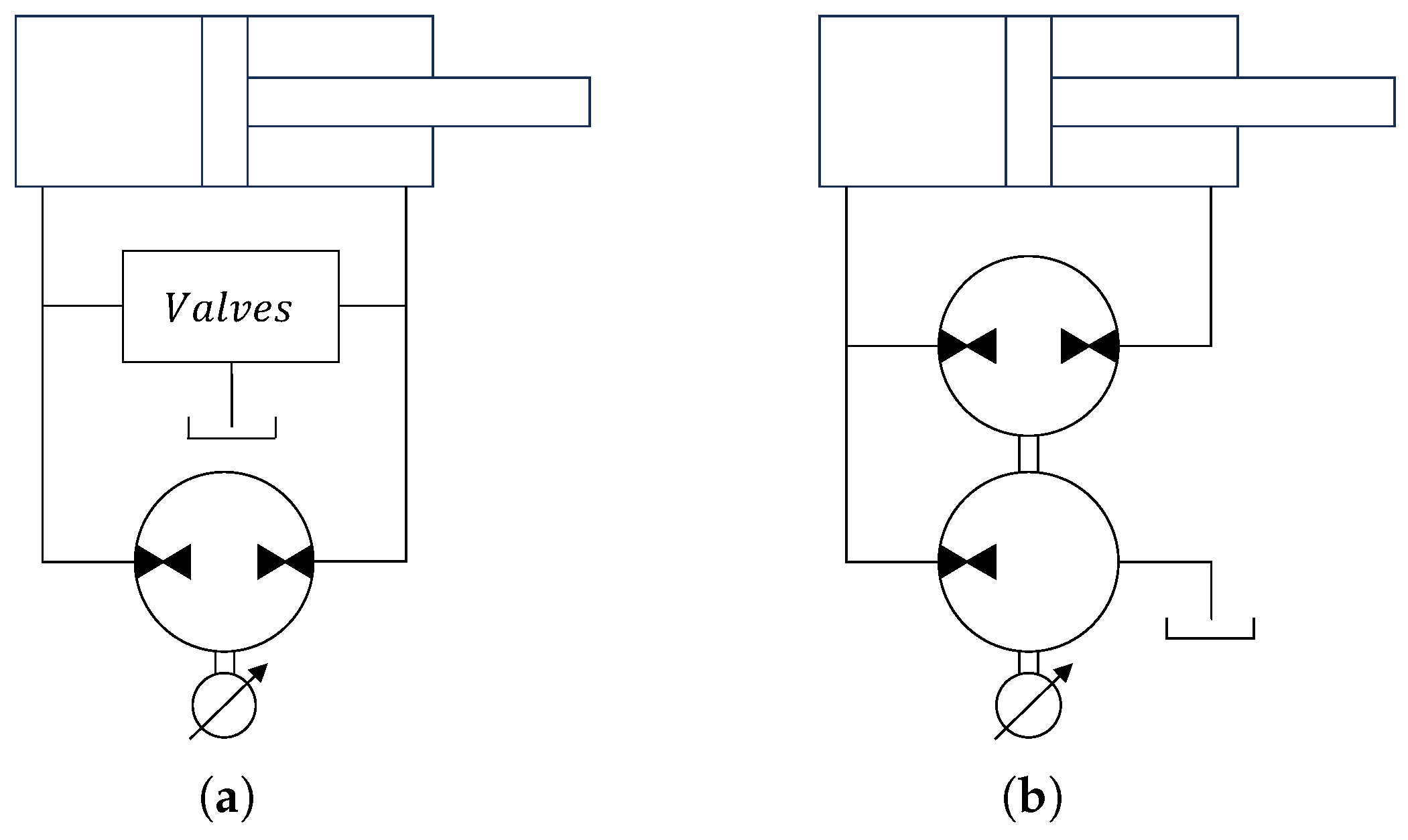
1. Introduction

Hydraulic actuation is a natural choice for linear motion control applications requiring precise control of large inertia loads. Advantages of hydraulic actuation include large force capabilities, high power density, and precise control, even when large inertia is involved. Traditional valve-controlled cylinders, however, suffer from several disadvantages relative to their electrical counterparts. These include lower energy efficiency, as well as increased commissioning time due to the installation of hydraulic piping. Pump-controlled cylinders are an emerging alternative that seeks to combine the advantages of these two technologies. By connecting a hydraulic pump directly to a hydraulic cylinder, the pump can be driven by a variable-speed electric motor, resulting in a highly energy-efficient solution due to the absence of fluid throttling associated with hydraulic control valves; see Figure 1. Furthermore, if the hydraulic reservoir is implemented using an accumulator, the result is a self-contained unit with a plug-and-play functionality that offers the advantages of hydraulic actuation, with an energy efficiency that may approach that of electrical actuators [1,2].

Feedback control is often required in practical applications, particularly for actuator position control. Classical feedback theory based on linear time-invariant (LTI) methods is the most widely used approach for the analysis and design of hydraulic control systems and has been well understood and applied to valve-controlled cylinders since the 1960s [3,4]. Despite this long and rich history filled with successful applications of LTI methods to hydraulic actuation systems, these systems are inherently non-linear with parameters that may exhibit strong time-varying characteristics. In particular, the effective bulk modulus of the fluid directly affects the dynamic performance of hydraulic actuators under feedback control. The effective bulk modulus quantifies the compressibility of the hydraulic fluid, where entrained air as well as the flexibility of the conduits are also accounted for [4]. Due to this compressibility, hydraulic systems exhibit resonant frequency response characteristics that may significantly limit the achievable performance under feedback control.

In general, the lower the effective bulk modulus for a given application, the lower the resonance frequency of the system, which necessitates the use of lower feedback gains in order to maintain stability. This results in slower response times and reduced performance under feedback control. For this reason, in many practical applications, especially where large inertia is involved, the achievable performance of a hydraulic actuator is dictated by the lowest occurring value of the effective bulk modulus. In practice, the value of the effective bulk modulus in a given system depends heavily upon pressure. The higher the pressure, the more air is dissolved into the fluid, leading to a higher bulk modulus and, thus, increased performance under feedback control. Furthermore, even though hydraulic cylinders have two pressure chambers, one on each side of the piston, it can be seen that these fluid volumes act as two springs in parallel, meaning that they can be thought of as a single spring with just one effective bulk modulus. For this reason, it is primarily the highest occurring pressure level in the two cylinder chambers that determines the lowest effective bulk modulus of the system. This means that even if one cylinder chamber pressure is low, a high effective bulk modulus may be achieved if the other cylinder chamber pressure is high [3,4].

For valve-controlled cylinders, the effective bulk modulus is always dictated by a high pressure level, assuming an adequate supply pressure. For a no-load condition (zero external force acting on the actuator), the pressures typically balance to a value close to half of the supply pressure due to valve leakage (e.g., close to 100 bar) [3,5], whereas for a large external force, the actuator pressure opposing the external force is at a high level. This results in a relatively high effective bulk modulus, where values above 6000 bar may be assumed with confidence [3]. In pump-controlled cylinders, however, the situation differs drastically. For commonly utilized circuits, such as the ones seen in Figure 1, the maximum occurring pressure in the system for a no-load condition is dictated by the reservoir pressure, which is typically implemented as a low-pressure accumulator pre-charged to a pressure level of between 1 and 10 bar [2,6,7] (1: This is achieved by replacing the open reservoir with an accumulator. 2: The use of such low pre-charge pressures is by necessity, as the accumulator must also serve as a drain line for the hydraulic pumps, which require a low-pressure connection.). In this article, pump-controlled cylinders operating with such low-pressure levels are referred to as low-pressure pump-controlled cylinders. As a result, the minimum occurring effective bulk modulus in low-pressure pump-controlled cylinders may be dictated by a pressure level as low as 1 bar, as opposed to, e.g., 100 bar in valve-controlled cylinders. Using the model utilized in [8], and assuming a gas fraction of one percent, this drastic reduction in actuator pressure conditions would theoretically lead to a decrease in the fluid’s effective bulk modulus from 6300 bar to 100 bar. This theoretical sixty-three-fold reduction in the minimum occurring effective bulk modulus of the actuator is expected to significantly degrade its performance under feedback control, and could even render the actuator ineffective when replacing a valve-controlled cylinder with a pump-controlled one. This assumes that the dynamics of pump-controlled cylinders are comparable to those of valve-controlled cylinders, which may or may not be the case, and applies to applications where the actuator experiences low external force conditions for at least part of its operating cycle.

From this, the following questions arise: How low must the effective bulk modulus be expected to fall in low-pressure pump-controlled cylinders, and how does this reduction impact the overall performance of the actuator under feedback control? Reviewing the available literature, no single research article has been located to provide a decisive answer to these questions. In [1], the performance of both circuits shown in Figure 1 was evaluated; however, this was conducted in the absence of feedback control and for an inertia of only slightly above 100 kg. In [9], the effective bulk modulus was estimated for a pump-controlled cylinder; however, only under the presence of a large external force, resulting in a very high effective bulk modulus comparable to that of valve-controlled cylinders. In [5,10], a pump-controlled circuit capable of replicating the pressure conditions of valve-controlled cylinders was presented; however, no experiments were provided quantifying the effective bulk modulus in low-pressure pump-controlled cylinders. In [8], the effective bulk modulus of a low-pressure pump-controlled cylinder was estimated using a theoretical model; however, these results remain uncertain until experimental investigations are provided. Lastly, studies on the effective bulk modulus in low-pressure hydraulic fluids have been conducted; see, e.g., [11]. However, it is uncertain how well the conditions of these experiments replicate the actual operating conditions of a pump-controlled cylinder under feedback control. The purpose of this paper is, therefore, to fill this gap by addressing these questions directly.

In this paper, the effective bulk modulus of low-pressure pump-controlled cylinders is studied. The minimal effective bulk modulus of a pump-controlled cylinder is identified under the minimal pressure conditions typical of these systems. The effects of the lowered effective bulk modulus—relative to valve-controlled cylinders—on the achievable performance and stability are studied in both the time and frequency domains for a system controlling a large inertia load with an effective inertia of above 10,000 kg. A feedback control design methodology based on a single worst-case operating point is proposed for these systems, and their ability to deliver adequate performance under feedback control for large inertia loads is assessed and validated experimentally. Additionally, critical modeling aspects commonly neglected in the literature are addressed, and their importance for the correct modeling of these systems is demonstrated. The results presented are of high importance for scenarios where pump-controlled cylinders are used with feedback control and should therefore be of high relevance to a wide range of applications.

The rest of this paper is organized as follows. Section 2 presents the experimental test rig and methodology, followed by modeling and parameter identification. Section 3 presents analytical and experimental results, followed by a discussion and conclusions in Section 4 and Section 5, respectively.

2. Materials and Methods

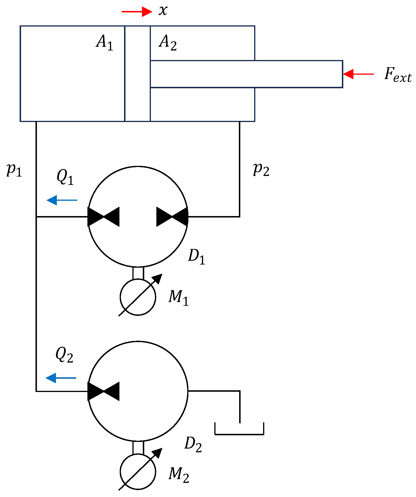
2.1. Experimental Test-Rig

The mechanical structure of the experimental test-rig and its degree of freedom is illustrated in Figure 2a. The mechanical system is a one-degree-of-freedom mechanism, which essentially functions like a seesaw; by extension/retraction of the hydraulic cylinder (x), the angle of the platform ($\theta$) may be increased/decreased. This test rig was constructed to represent a single degree of freedom of a wave compensation platform, which is used in marine and offshore applications to keep critical equipment horizontal on vessels influenced by wave motion.

In addition to the rotating mechanical top plate itself, 12 weight plates (shown in red in Figure 2b, each with a mass of $m=58 \mathrm{kg}$, are placed on either side of the top plate to simulate a large inertia load. The resulting inertia of the rotating parts about their center of rotation is extracted from the CAD model of the system as $I=2648 {\mathrm{kgm}}^2$. With the cylinder placed at a distance of $r=0.5\mathrm{m}$, the cylinder then experiences an effective mass of $m_{eff}=I/r^2=\mathrm{10,593} \mathrm{kg}$. Due to the balanced load conditions, the external force acting on the cylinder is zero at the horizontal position and near zero for small perturbations of the cylinder.

The hydraulic cylinder used is a pump-controlled cylinder. Since the cylinder is an asymmetrical cylinder ($A_1\ne A_2$), which is common in most industrial applications, the hydraulic circuit needs to accommodate the asymmetrical flow of the actuator. This may be conducted either using a single-pump solution and an auxiliary valve arrangement, as shown in Figure 1a, or a dual-pump solution, as shown in Figure 1b. For this system, a dual-pump solution was utilized to handle the asymmetrical flow; the hydraulic circuit architecture is shown in Figure 3.

Additionally, the pump-controlled cylinder is implemented as a dual prime mover (DPM) circuit, where the velocity of each pump is controlled individually by dedicating one prime mover for each pump. This provides an extra degree of freedom in the control system, which may be utilized to manipulate the pressure conditions of the actuator. The DPM circuit modification was originally introduced to control the pressure conditions of the actuator so as to mimic those of traditional valve-controlled cylinders (i.e., providing large actuator pressures even with zero external force); see [5,10]. However, here it is used for a different purpose. Referring back to the two methods of handling the asymmetrical flow of the actuator, neither solution provides ideal conditions for identifying the effective bulk modulus under low external force conditions. The single-pump solution inherently suffers from non-linear switching dynamics under low-force conditions, which significantly impacts the actuator’s behavior and may often lead to instability even in the absence of feedback control; see, e.g., [12]. The dual-pump solution does not suffer from this phenomenon; however, due to non-ideal matching of the displacements of the pump and the pump’s leakage characteristics, unpredictable pressure phenomena may arise during operation [2]. For this reason, the circuit is implemented as a DPM circuit, with the pressure control algorithm described in Section 2.3 utilized to ensure the typical minimal operating pressures found in low-pressure pump-controlled cylinders (e.g., 4–5 bar). The advantage of using a DPM circuit for this purpose is that it ensures continuous and stable pressure dynamics, facilitating accurate identification of the effective bulk modulus.

The prime movers utilized are commercially available servo motors (permanent magnetic synchronous motors), each driven by a separate commercially available servo drive. The motors are identical to each other, both with rated torques and rated angular velocities of $T_{motor}=12.5\mathrm{Nm}$ and $n_{motor}=3000\mathrm{rev}/\min$, respectively. The main pump (driven by motor $M_1$ in Figure 3) is an axial piston pump with a displacement of $D_1=6 {\mathrm{cm}}^3/\mathrm{rev}$ and a maximum angular velocity of $n_{p1}=3600\mathrm{rev}/\min$. The secondary pump (driven by motor $M_2$ in Figure 3) is an internal gear pump with a displacement of $D_1=3.6 {\mathrm{cm}}^3/\mathrm{rev}$ and a maximum angular velocity of $n_{p2}=3600\mathrm{rev}/\min$. The control system is implemented on an industrial PLC with a sampling frequency of $100\mathrm{Hz}$ for both the control system as well as for data acquisition. The rest of the system parameters are presented in Section 2.3.

2.2. Methodology

For control design and analysis, the focus of this paper is on classical feedback theory using LTI models, due to its widespread use in both industry and academia. Hydraulic systems are inherently time-variant systems, and therefore, the time-varying nature of the parameters must be accounted for in the control design. Traditionally, for valve-controlled systems, this is done by determining the worst-case operating point in terms of stability and performing control design and analysis for this point. For hydraulic systems, this corresponds to the operating point with the lowest bulk modulus, the lowest leakage, and the highest gain. For valve-controlled systems specifically, the lowest leakage and highest gain coincide at a single point, namely, near or at zero valve opening, meaning near or at zero velocity. This is due to the linearization coefficients and the nature of valve leakage [3]. In pump-controlled cylinders, on the other hand, there are no valve linearization coefficients, and thus the question arises: what operating point should be used?

First, considering the effective bulk modulus, it is obvious that the operating point with the lowest external force, $F_{ext}$, should be utilized in low-pressure pump-controlled cylinders, due to the relation between the effective bulk modulus and pressure. Furthermore, an operating point with low acceleration should be used. This ensures that the pressures of the actuator are kept near their minimum values, which is where the lowest effective bulk modulus occurs. Considering this parameter alone, a natural candidate for control design and analysis in these systems is a low-amplitude step signal. Secondly, regarding leakage, unlike valve-controlled systems, no general statement can be made about the minimal leakage operating point for pump-controlled systems. As shown in [13], external pump leakage tends to increase for increasing rotational velocities, whereas the internal pump leakage tends to decrease for increasing rotational velocities. Additionally, most commercially available pumps are not able to ensure proper operation at very low speeds, resulting in deadband-like behavior at low speeds [13]. Because of these factors, identifying the operating point where minimal leakage occurs may prove extremely challenging in most applications without the use of specialized instrumentation not typically available in real-world settings. For this reason, an approach to control design and analysis based on a single operating point is proposed and presented here.

The proposed method for control design and analysis in low-pressure pump-controlled cylinders is as follows:

• Establish an LTI model of the system.
• Record the system’s response to a small-stroke (low-amplitude) step signal with the minimum external force acting on the cylinder.
• Perform parameter identification for this operating point (bulk modulus, pump leakage, and viscous friction).
• Assume this operating point is the worst-case with respect to stability (i.e., the lowest occurring leakage).
• Design a feedback controller with low stability margins (e.g., a phase margin of less than 40 degrees) for this operating point.
• Investigate if the system remains stable for large-stroke signals.

If this method results in a stable system for large-stroke signals, the proposed operating point is, in fact, for all intents and purposes, the worst-case operating point in terms of stability, and may be used for control design and analysis. The designer may then design a feedback controller based on what is considered adequate stability margins for the given system at hand. If, however, this process results in an unstable system, the proposed solution is to decrease the estimate for the lowest occurring leakage by a certain amount and repeat the process until a stable system response is achieved. Although not mathematically rigorous, the proposed method may perhaps be the best solution one can achieve in most practical applications.

Regarding the selection of the size of the step signal, as mentioned previously, it should be as small as possible; however, it should be sufficiently large as to have the pump(s) operate outside of their deadband-like regions for parts of the step response. Due to the way most commercially available pumps operate near zero velocity, it is expected that the response of an overshooting feedback controller will suddenly become significantly damped as the system begins to settle and the pump approaches its deadband-like region. With this in mind, the methodology used in this paper for identifying the effective bulk modulus of the pump-controlled cylinder is as follows:

• A step signal is designed according to the aforementioned guidelines.
• A proportional controller sufficiently large to produce a pronounced overshoot of the system is implemented.
• The step response of the system is recorded, referred to henceforth as the identification set.
• A parameter optimization routine is utilized to determine the value of the effective bulk modulus (and possibly other uncertain parameters) by comparing the experimental response with that of the LTI model.

Additionally, to minimize the risk of over-tuning, a second dataset is recorded and utilized in the parameter optimization process, referred to as the validation set.

2.3. Modeling

2.3.1. Linear Time-Invariant Model

Referring to Figure 3, Newton’s second law applied to the cylinder gives the following:

$$m\ddot{x}=p_1{A}_1-p_2{A}_2-F_{ext}-b\dot{x}$$

(1)

where m is the combined mass of the cylinder piston and mechanical load, $p_1$ and $p_2$ are the pressures of the actuator, $A_1$ and $A_2$ denote the areas of the cylinder, and b denotes the viscous friction coefficient. Applying the continuity equation to $p_1$ and $p_2$, we have the following:

$$\begin{array}{cc}\hfill {\dot{p}}_1& ={\displaystyle \frac{\beta }{V_1}}\left(D_1{\omega }_1+D_2{\omega }_2-A_1\dot{x}-Q_{L1}\right)\hfill \end{array}$$

(2)

$$\begin{array}{cc}\hfill Q_{L1}& =c_1{p}_1+c_{12}(p_1-p_2)\hfill \end{array}$$

(3)

$$\begin{array}{cc}\hfill {\dot{p}}_2& ={\displaystyle \frac{\beta }{V_2}}\left(-D_1{\omega }_1+A_2\dot{x}-Q_{L2}\right)\hfill \end{array}$$

(4)

$$\begin{array}{cc}\hfill Q_{L2}& =c_2{p}_2-c_{12}(p_1-p_2)\hfill \end{array}$$

(5)

where $\beta$ is the effective bulk modulus of the fluid. $D_1$ and $D_2$ are the displacements of the primary and secondary pumps, respectively. ${\omega }_1$ and ${\omega }_2$ are the rotational velocities of the primary and secondary pumps, respectively. $c_1$, $c_2$, and $c_{12}$ are the leakage coefficients. $V_1$ and $V_2$ are the volumes of the actuator, given by the following:

$$\begin{array}{cc}\hfill V_1& =V_{L1}+A_{1}x\hfill \end{array}$$

(6)

$$\begin{array}{cc}\hfill V_2& =V_{L2}+A_2(x_{max}-x)\hfill \end{array}$$

(7)

where $V_{L1}$ and $V_{L2}$ are the line volumes and $x_{max}$ is the maximum stroke of the cylinder. Applying Newton’s second law to the electric motors, we have the following:

$$\begin{array}{cc}\hfill J_1\dot{{\omega }_1}& ={\tau }_{em1}-D_1(p_1-p_2)\hfill \end{array}$$

(8)

$$\begin{array}{cc}\hfill J_2\dot{{\omega }_2}& ={\tau }_{em2}-D_2{p}_1\hfill \end{array}$$

(9)

where $J_1$ is the combined inertia of the primary motor and pump, and $J_2$ is the combined inertia of the secondary motor and pump. Note that the viscous damping term of the motors has been neglected, as is common practice due to its small influence relative to the velocity feedback of the motors [14]. ${\tau }_{em1}$ and ${\tau }_{em1}$ are first-order approximations for the current dynamics of the motors, given by the following:

$$\begin{array}{cc}\hfill {\displaystyle \frac{{\tau }_{em1}}{{\tau }_{ref1}}}\left(s\right)& ={\displaystyle \frac{1}{s/{\omega }_I+1}}\hfill \end{array}$$

(10)

$$\begin{array}{cc}\hfill {\displaystyle \frac{{\tau }_{em2}}{{\tau }_{ref2}}}\left(s\right)& ={\displaystyle \frac{1}{s/{\omega }_I+1}}\hfill \end{array}$$

(11)

where ${\tau }_{ref1}$ and ${\tau }_{ref2}$ are the reference torques of the primary and secondary motors, respectively, and ${\omega }_I$ is the reciprocal of the time constant of the current dynamics. Furthermore, the motors are velocity controlled, where proportional feedback controllers are assumed, as follows:

$$\begin{array}{cc}\hfill {\tau }_{ref1}& =K_{m1}({\omega }_{1ref}-{\omega }_1+u_{ff1})\hfill \end{array}$$

(12)

$$\begin{array}{cc}\hfill {\tau }_{ref2}& =K_{m2}({\omega }_{2ref}-{\omega }_2+u_{ff2})\hfill \end{array}$$

(13)

where $K_{m1}$ and $K_{m2}$ are the proportional feedback controllers of the primary and secondary motors, respectively, and ${\omega }_{1ref}$ and ${\omega }_{2ref}$ are the velocity references of the primary and secondary motors, respectively. $u_{ff1}$ and $u_{ff2}$ are velocity feedforwards implemented by the manufacturer of the servo drives, applied to each electric motor from the reference inputs (${\omega }_{1ref}$ and ${\omega }_{2ref}$) to the reference torques (${\tau }_{ref1}$ and ${\tau }_{ref2}$) in the following manner:

$$\begin{array}{cc}\hfill u_{ff1}\left(s\right)& ={\displaystyle \frac{K_{ff}}{{\tau }_{ff}s+1}}{\dot{\omega }}_{1ref}\hfill \end{array}$$

(14)

$$\begin{array}{cc}\hfill u_{ff2}\left(s\right)& ={\displaystyle \frac{K_{ff}}{{\tau }_{ff}s+1}}{\dot{\omega }}_{2ref}\hfill \end{array}$$

(15)

where $K_{ff}$ and ${\tau }_{ff}$ are the feedforward gain and filter constant, respectively. In order to control the cylinder velocity as a single-input single-output (SISO) system, the following motor control laws are implemented: [5,10,15]:

$$\begin{array}{cc}\hfill {\omega }_{1ref}\left(s\right)& =K_{scale}u\hfill \end{array}$$

(16)

$$\begin{array}{cc}\hfill {\omega }_{2ref}\left(s\right)& ={\omega }_{1ref}\alpha \hfill \end{array}$$

(17)

where u is the reference velocity of the cylinder, $K_{scale}$ is a scaling factor converting between normalized SI units and the units utilized by the PLC, and $\alpha$ is a factor ensuring that the pump output flows are matched to the area ratio ($A_2/A_1$) of the cylinder:

$$\begin{array}{cc}\hfill \alpha & ={\displaystyle \frac{D_1}{D_2}}\left({\displaystyle \frac{A_1}{A_2}}-1\right)\hfill \end{array}$$

(18)

The extra degree of freedom achieved by the DPM circuit is utilized to control the sum of the pressures, as is commonly done [5,10,15]:

$$\begin{array}{cc}\hfill u_{p1}& =K_{pres}(p_{sum,ref}-p_{sum})\hfill \end{array}$$

(19)

$$\begin{array}{cc}\hfill u_{p2}& =K_{pres}{K}_{\beta }(p_{sum,ref}-p_{sum})\hfill \end{array}$$

(20)

where $u_{p1}$ and $u_{p2}$ are control effort components of the sum pressure control law, $K_{pres}$ is the sum pressure gain, $K_{\beta }$ is a scaling factor to be discussed in a later section, $p_{sum}$ is the sum of the pressures ($p_1+p_2$), and $p_{sum,ref}$ is the setpoint for the sum of the pressures. Proportional feedback control of the cylinder’s position may then be implemented in the following manner:

$$\begin{array}{cc}\hfill u_1& =K_p(x_{ref}-x)-u_{p1}\hfill \end{array}$$

(21)

$$\begin{array}{cc}\hfill u_2& =K_p\alpha (x_{ref}-x)+u_{p2}\hfill \end{array}$$

(22)

where $K_p$ is the proportional feedback gain, and $x_{ref}$ is the reference position.

Although inherently a multiple-input multiple-output (MIMO) system, due to the control law implementation, the resulting system functions as a decoupled SISO system from reference input to the output cylinder velocity/position [16]. The pump-controlled cylinder is then a SISO velocity source from reference input (u) to the output velocity of the cylinder $\dot{x}$, open-loop. The cylinder may then be position-controlled using any control law (e.g., a proportional feedback controller) and treated as an SISO system.

Additionally, due to the sum pressure control law, the sum of the actuator pressures ($p_1+p_2$) is controlled to follow the desired reference setpoint $p_{sum}$, which will be utilized here to ensure that the pressures remain within the typical operating range of low-pressure pump-controlled cylinders (e.g., 1–10 bar).

2.3.2. Leakage Model

As will be seen in Section 2.4, due to pump leakage, the motor/pump velocities are non-zero when the cylinder is maintained at a stationary position under feedback control. This information will be utilized in Section 2.4 in order to facilitate the identification of pump leakages coupled with the equations to be presented here.

Referring to Figure 3, due to the flow continuity of the control volumes $p_1$ and $p_2$, for zero-cylinder velocity, we have the following:

$$\begin{array}{cc}\hfill D_1{\omega }_1+D_2{\omega }_2-c_1{p}_1-c_{12}(p_1-p_2)& =0\hfill \end{array}$$

(23)

$$\begin{array}{cc}\hfill -D_1{\omega }_1+c_{12}(p_1-p_2)-c_2{p}_2& =0\hfill \end{array}$$

(24)

For a given value of $c_{12}$, the remaining leakage coefficients may then be identified for a given stationary operating point utilizing measurements of the motor/pump velocities (${\omega }_1$, ${\omega }_2$) and the steady-state pressures ($p_1$ and $p_2)$ using Equations (23) and (24) as follows:

$$\begin{array}{cc}\hfill c_1& ={\displaystyle \frac{1}{p_1}}\left(D_2·{\omega }_2-c_{12}(p_1-p_2)+D_1{\omega }_1\right)\hfill \end{array}$$

(25)

$$\begin{array}{cc}\hfill c_2& ={\displaystyle \frac{1}{p_2}}\left(-D_1{\omega }_1+c_{12}(p_1-p_2)\right)\hfill \end{array}$$

(26)

As a result, only one leakage parameter ($c_{12}$) will have to be identified.

2.3.3. Block Diagram and Transfer Function

Next, in order to extract a transfer function based on the governing equations of the system, Equations (1)–(22) are Laplace-transformed and combined as a block diagram. Figure 4 shows the block diagram implemented in Simulink without the sum pressure control algorithm included, where the following definitions have been introduced:

$$\begin{array}{cc}\hfill G_1& =K_p{K}_{scale}\hfill \end{array}$$

(27)

$$\begin{array}{cc}\hfill G_2& ={\displaystyle \frac{K_{ff}s}{{\tau }_{ff}s+1}}\hfill \end{array}$$

(28)

$$\begin{array}{cc}\hfill G_3& ={\displaystyle \frac{1}{s/{\omega }_I+1}}\hfill \end{array}$$

(29)

$$\begin{array}{cc}\hfill G_4& ={\displaystyle \frac{1}{J_{1}s}}\hfill \end{array}$$

(30)

$$\begin{array}{cc}\hfill G_5& ={\displaystyle \frac{1}{J_{2}s}}\hfill \end{array}$$

(31)

$$\begin{array}{cc}\hfill G_6& ={\displaystyle \frac{\beta }{V_{1}s}}\hfill \end{array}$$

(32)

$$\begin{array}{cc}\hfill G_7& ={\displaystyle \frac{\beta }{V_{2}s}}\hfill \end{array}$$

(33)

$$\begin{array}{cc}\hfill G_8& ={\displaystyle \frac{1}{ms}}\hfill \end{array}$$

(34)

Due to the complex interaction of the equations, an analytic transfer function from the reference input to the output of the system is not easily obtained. The authors were unable to do so manually via block diagram manipulations, and were also unable to do so using numerical software. For this reason, LTI simulation and analysis are carried out in the following manner:

• For SISO LTI analysis in the frequency domain, a numerical transfer function is obtained by using the block diagram of Figure 4 after entering numerical values for each parameter utilizing MATLAB R2021b ’s linmod command. For open-loop frequency responses, the lowest feedback branch in Figure 4 is removed.
• For time-domain simulation (step responses), the block diagram of Figure 4 is utilized with the addition of the sum pressure control loop. The simulations are executed in Simulink, and the results are exported to MATLAB’s workspace for post-processing.

Figure 4. Block diagram implementation of the governing equations in Simulink.

Figure 4. Block diagram implementation of the governing equations in Simulink.

2.3.4. Parameters

The cylinder areas $A_1$ and $A_2$ are evaluated using the following:

$$\begin{array}{cc}\hfill A_1& ={\displaystyle \frac{1}{4}}\pi d_1^2\hfill \end{array}$$

(35)

$$\begin{array}{cc}\hfill A_2& ={\displaystyle \frac{1}{4}}\pi d_1^2-{\displaystyle \frac{1}{4}}\pi d_2^2\hfill \end{array}$$

(36)

where $d_1$ and $d_2$ are the piston and rod diameters, respectively. The inertias $J_1$ and $J_2$ are evaluated using the following:

$$\begin{array}{cc}\hfill J_1& =J_{m1}+J_{p1}\hfill \end{array}$$

(37)

$$\begin{array}{cc}\hfill J_2& =J_{m2}+J_{p2}\hfill \end{array}$$

(38)

where $J_{m1}$ and $J_{m2}$ are the rotor inertias of the electric motors, and $J_{p1}$ and $J_{p2}$ are the inertias of the primary and secondary pumps, respectively. The current dynamics of the electric motors are assumed to have a time constant of 200 Hz. The feedforward gain of the electrical motors is matched to the rotor inertia of the motors, i.e., $K_{ff}=J_{m1}=J_{m2}$. The other known system parameters that have not yet been mentioned are given in

Table 1. Parameters of the pump-controlled cylinder.

Parameter	Value	Unit
$d_1$	63	mm
$d_2$	36	mm
$V_{L1}=V_{L2}$	0.1272	dm3
$x_{max}$	500	mm
$J_{m1}=J_{m2}$	1600	kgmm2
$J_{p1}$	600	kgmm2
$J_{p2}$	34	kgmm2
${\omega }_I$	1256.6	1/s
${\tau }_{ff}$	0.0012	1/s
$K_{scale}$	314.1593	-

. The remaining system parameters are to be identified or determined in the following sections. Additionally, for the experiments to be presented, the setpoint of the sum pressure algorithm will be set to 10 bar. $K_{\beta }$ is a tuning factor that optimizes the behavior of the sum pressure algorithm, set to 1.4 in the experiments to be presented. Lastly, the gain of the sum pressure algorithm will be set to 22 for inertia loads above 10 tons and 15 for lower inertias.

2.4. Parameter Identification

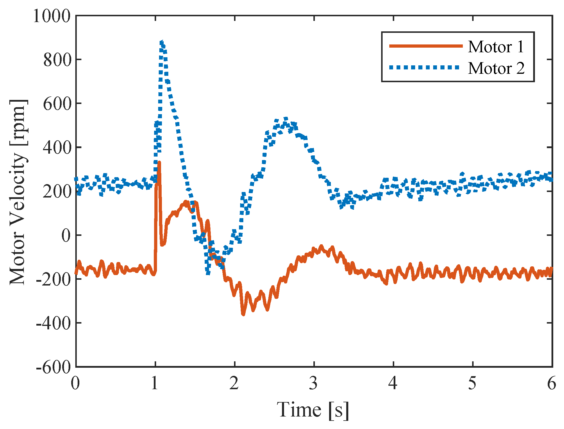
2.4.1. Electric Drive

For the tuning of the velocity feedback controller on the electric drive, an automated routine is implemented by the manufacturer. During commissioning of the system, this routine was executed with the motors decoupled from the hydraulic pumps. As a result, the servo drives tune the feedback controllers of the motors based on the inertia of the motors only. The solid line (“Exp”) of Figure 5 shows the response of one of the electric motors to a step signal (voltage input to the electric motor), where the response was filtered using a zero-phase Butterworth filter with a cut-off frequency of 10 Hz. As can be seen in Figure 5, the electric motor achieves a very fast response time, settling after approximately 0.2 s.

Next, the response of the electric motor can be modeled by combining Equations (8), (10) and (12), where the second and last terms of Equations (8) and (13) are omitted, respectively. By replacing $J_1$ with $J_{m1}$, the conditions of the experimental step response may be simulated with the only unknown variable being $K_{m1}$. This feedback control gain is set automatically on the servo drive, but it is only made available to the user as a normalized value, and its numerical value must, therefore, be identified. Fortunately, there is only one unknown parameter in this case, and the identification of this parameter is, therefore, straightforward.

The dotted line (“LTI”) in Figure 5 shows the response of the LTI model achieved by combining Equations (8), (10) and (12) for $K_{m1}=0.026$. As can be seen in the figure, the lines almost perfectly overlap; therefore, the proportional feedback controller of the electric motors is taken as $K_{m1}=K_{m2}=0.026$. Please note that the experimental response in Figure 5 is acquired with the velocity feedforward of the electric drive being inactive.

2.4.2. Identification and Validation Data

Next, identification data is gathered by recording the step response of the cylinder to a 5 mm step change from 340 mm to 345 mm (mid stroke, horizontal platform) using a proportional position feedback controller of $K_p$ = 25 rad/(m·s). This is done with the system loaded with the maximum number of weight plates (12 on either side), resulting in an effective mass of $m_{eff}$ = 10,593 kg. The solid line (Exp) in Figure 6 shows the response of the system. The pressures and motor/pump velocities during the step response are given in Figure 7 and Figure 8, respectively, where the pressures are filtered in the same manner as the response of the electric drive.

In Figure 6, a drastic change is observed in the system’s behavior, approximately 2.2 s after the step command. This is due to the increased leakage and non-linear pump characteristics that occur for low pump velocities as the system starts to settle, as discussed in Section 2.2. The region beyond this point (indicated by the horizontal line at $t=3.2\mathrm{s}$) is referred to here as the non-LTI region. Observe that the increased leakage at lower pump velocities has a stabilizing effect on the system. For LTI parameter identification, it is only the part of the system response that occurs prior to the non-LTI region that will be considered.

Next, for the validation set, the gain of the feedback controller is lowered slightly, producing the response depicted by the solid line (“Exp”) in Figure 9 using $K_p=20$. As with the previous step response, the nonlinear characteristics of the pump dominate at low motor/pump velocities, which occur here approximately 1.9 s after the step command.

Finally, in addition to the identification and validation sets, a third dataset will be used for further validation of the LTI model and its parameters, referred to here as the robustness set. For the robustness set, a significant change in the mechanical system is introduced by reducing the number of weight plates on both sides to five. This reduces the effective mass experienced by the cylinder to $m_{eff}=4898\mathrm{kg}$. The step response of the experimental system with this reduced load is shown in Figure 10 for a $K_p$ value of 40.

2.4.3. Leakage Identification

In Figure 8, it can be seen that with the cylinder stationary, the motor/pump velocities are non-zero. As discussed in Section 2.3, this is due to pump leakage. For calculation of the leakage coefficients $c_1$ and $c_2$, the pump velocities at standstill ($x=345\mathrm{mm}$) are utilized (${\omega }_1=-160\mathrm{rpm}$ and ${\omega }_1=245\mathrm{rpm}$) along with $p_1=3.95 \mathrm{bar}$. For leakage identification, the pressure $p_2$ is evaluated using the steady-state force balance:

$$\begin{array}{cc}\hfill p_1{A}_1-p_2{A}_2+F_{ext}& =0\hfill \end{array}$$

(39)

The reason for evaluating $p_2$ from force balance is that discrepancies not accounted for in an LTI model affect the pressures, changing them slightly (e.g., nonlinear friction, sensor inaccuracies). For $F_{ext}=0$ ($x=345\mathrm{mm}$), the pressure $p_2$ evaluates to 5.86 bar. This information is then utilized along with (25) and (26) in the following in order to evaluate $c_1$ and $c_2$ for a given value of $c_{12}$.

2.4.4. Grid Search Optimization

The unknown parameters to be identified are as follows: the effective bulk modulus $\beta$, the pump leakage coefficient $c_{12}$, and the viscous friction b. Due to the low number of unknown parameters, grid search optimization is selected for parameter identification and is carried out in the following manner:

• A lower and upper bound are defined for each unknown parameter, resulting in a continuous range.
• The continuous range is then discretized for each parameter.
• Using the discretized range for each parameter, all possible combinations of the parameters (referred to as the grid) are then simulated, and the results are recorded and compared to the experimental data.

For evaluating each point in the grid, the mean squared error (MSE) of the difference between the experimental and simulated (LTI) step responses is evaluated. For any point in the grid, this is conducted for both the identification set and the validation set, and the average of these two is used to assess each point in the grid.

Furthermore, the grid search optimization is carried out in two steps. First, a wide grid is utilized using a wide range for each unknown parameter. Thereafter, a second grid is utilized (referred to as the refined grid), based on the results of the first grid.

For the first grid, the upper and lower bounds are as follows:

• $25\mathrm{bar}\le \beta \le 1000\mathrm{bar}$
• $50\mathrm{Ns}/\mathrm{m}\le b\le 500\mathrm{Ns}/\mathrm{m}$
• 1·${10}^{-13}{\mathrm{m}}^5/\left(\mathrm{Ns}\right)\le c_{12}\le$1·${10}^{-9}{\mathrm{m}}^5/\left(\mathrm{Ns}\right)$

The upper bound on $\beta$ is selected based on theoretical considerations and is considered more than justified, considering the low operating pressures. For the discretization, $\beta$ is incremented in steps of 25 up to 250, then steps of 50 up to 300, then steps of 100 up to 600, and then steps of 200 up to 1000. b is incremented in steps of 25 up to 250, then steps of 50 up to 300, and then steps of 100 up to 500. This results in a parameter grid of 3264 possible combinations, all of which are evaluated as described previously.

Next, grid search optimization is executed using MATLAB and Simulink. The best solution resulting from the first grid has an MSE of 0.0694. Excluding all solutions with an MSE greater than 0.25, 48 solutions are left, all of which have the three unknown parameters within the following bounds:

• $150\mathrm{bar}\le \beta \le 200\mathrm{bar}$
• $200\mathrm{Ns}/\mathrm{m}\le b\le 500\mathrm{Ns}/\mathrm{m}$
• 1·${10}^{-10}{\mathrm{m}}^5/\left(\mathrm{Ns}\right)\le c_{12}\le$1·${10}^{-10}{\mathrm{m}}^5/\left(\mathrm{Ns}\right)$

Based on these results, the refined grid for the second grid search optimization is selected as follows:

• $130\mathrm{bar}\le \beta \le 220\mathrm{bar}$
• $100\mathrm{Ns}/\mathrm{m}\le b\le 600\mathrm{Ns}/\mathrm{m}$
• $0.8$·${10}^{-10}{\mathrm{m}}^5/\left(\mathrm{Ns}\right)\le c_{12}\le$$2.4$·${10}^{-10}{\mathrm{m}}^5/\left(\mathrm{Ns}\right)$

where the parameters are discretized as follows: $\beta$ is incremented in steps of 5 from its lower to its upper bound, b is incremented in steps of 50 from its lower to its upper bound, and $c_{12}$ is discretized using 17 equally spaced points. This results in a refined grid with a total of 3553 combinations to be evaluated.

Evaluating all solutions in the refined grid, the best solution has an average MSE of 0.0353 (compared to 0.0694 from the preliminary grid). This solution is taken as the final solution, and the values for the parameters that are to be determined are as follows:

• $\beta =165\mathrm{bar}$
• $b=100\mathrm{Ns}/\mathrm{m}$
• $c_{12}=1.2$·${10}^{-10}{\mathrm{m}}^5/\left(\mathrm{Ns}\right)$

with the leakage coefficients $c_1$ and $c_2$ as follows:

• $c_1=5.49$·${10}^{-11}{\mathrm{m}}^5/\left(\mathrm{Ns}\right)$
• $c_2=-1.19$·${10}^{-11}{\mathrm{m}}^5/\left(\mathrm{Ns}\right)$

Notice the negative sign of $c_2$. The physical explanation for this is as follows: The leakage flow proportional to $c_{12}$ is actually negative (flowing into the control volume $p_2$). Additionally, it appears that there is a slight null shift in the pumps’ velocity-flow characteristics, where it provides more flow than what is expected for the operating conditions utilized in the leakage identification. In this case, the leakage coefficient $c_2$ models both leakage from $p_1$ to the reservoir and the surplus flow resulting from the null shift.

The resulting step responses using the developed LTI model with the identified parameters are depicted by the dotted lines (“LTI”) of Figure 6 and Figure 9 for the identification and validation sets, respectively. As can be seen from the figures, the LTI model closely matches that of both the identification and validation sets up to the onset of the non-LTI region. The agreement between the LTI model and the experimental results is considered satisfactory.

Furthermore, to provide additional validation of the developed model and the identified parameter set, the response of the model is evaluated using $m_{eff}=4898\mathrm{kg}$ and compared to that of the robustness set. It should be noted here that some minor variations in system parameters are expected in the robustness set for the effective bulk modulus as well as for the pump leakages. This is due to the following factors: First of all, although the identification and validation sets were recorded back to back, the data for the robustness had to be recorded after the system had been shut down for a lengthy duration. The reason for this is that due to safety regulations, the system had to be shut down before removing the weight plates. This is a time-consuming process, meaning that the system experienced lengthy downtime before being started again. For this reason, the amount of entrained and undissolved air in the system might have varied slightly. Secondly, for the lowered effective inertia, the step response is more rapid, meaning that the motors move faster. In such a situation, the leakage characteristics are expected to differ slightly. With this in mind, minor variations in $\beta$ and $c_{12}$ were introduced in order to achieve the results of Figure 10, where $\beta =220\mathrm{bar}$ and $c_{12}=1.0$·${10}^{-10}{\mathrm{m}}^5/\left(\mathrm{Ns}\right)$ were utilized for the LTI model, as opposed to $\beta =165\mathrm{bar}$ and $c_{12}=1.2$·${10}^{-10}{\mathrm{m}}^5/\left(\mathrm{Ns}\right)$. The agreement between the LTI model and the experimental system’s response can be observed in Figure 10, where it is again seen that the LTI model closely follows the experimental system’s response up to the non-LTI region.

Lastly, attention is brought here to the effects of the velocity feedforward of the electric drive, described in Section 2.3. Such feedforwards are likely found on all commercially available servo drives; however, they are commonly neglected in the literature on pump-controlled cylinders (see, e.g., [5,9,17,18,19,20]). In fact, the authors have yet to come across another publication on a pump-controlled cylinder where this feedforward has been included in the model. As seen in Figure 11, the impact of this feedforward is drastic. Figure 11 compares the step response of the developed LTI model (“LTI”) with that of the same model but with the feedforward neglected (“LTI2”). As can be seen from the figure, neglecting the feedforward not only results in a much higher overshoot of the system, but also in a delayed system response. The consequence of neglecting this critical aspect of the system in any model (LTI model or otherwise) should, therefore, not be taken lightly, as it would result either in an incorrect model or incorrectly identified parameters.

3. Results

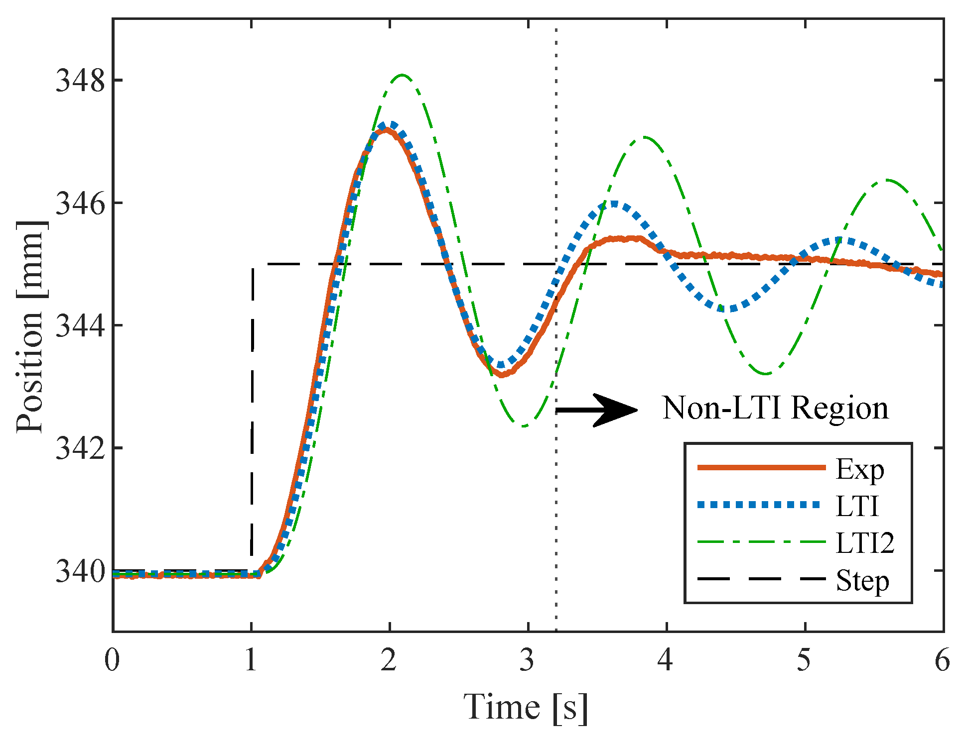
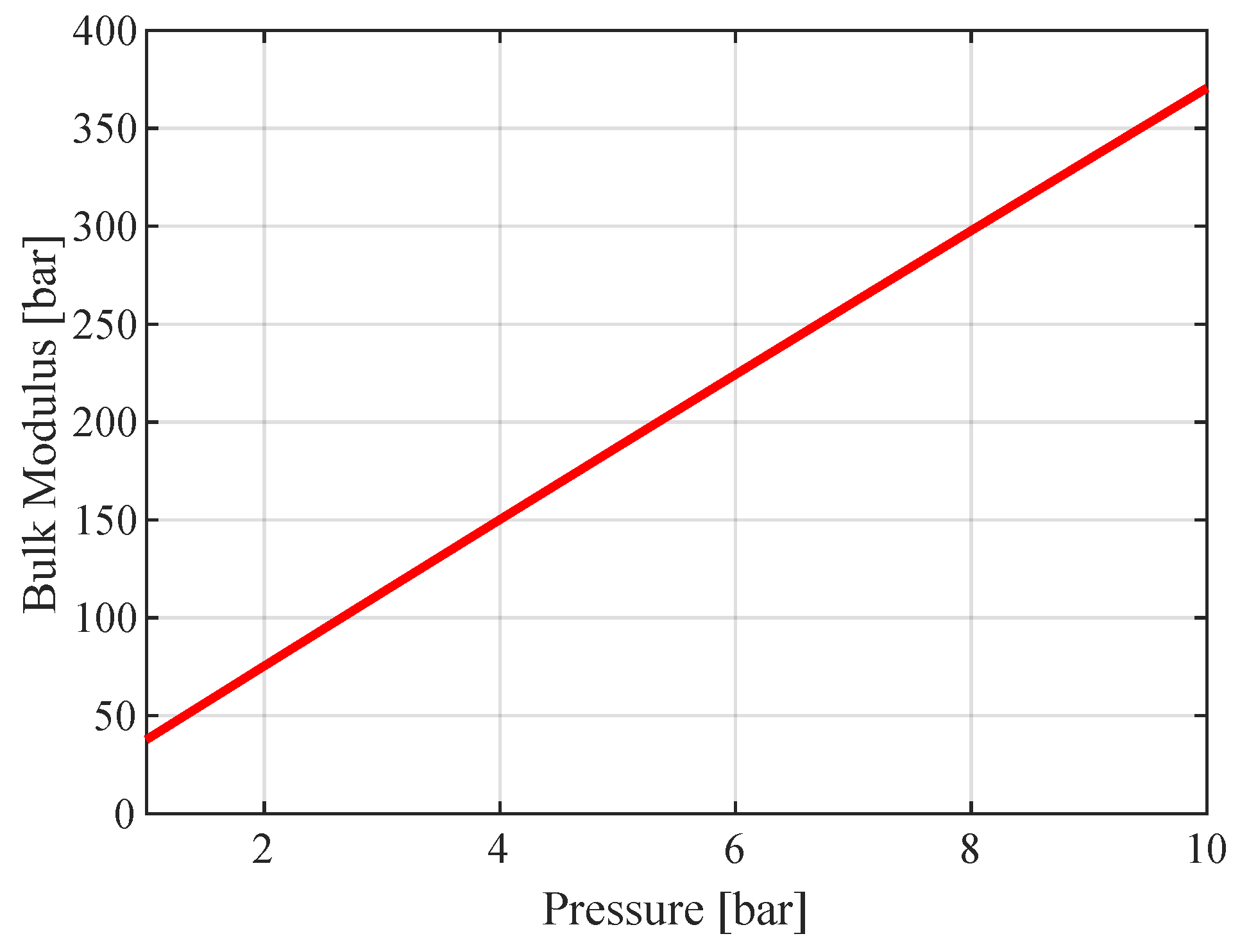
3.1. Bulk Modulus

As seen in the previous section, the effective bulk modulus of the system was identified at $\beta =165\mathrm{bar}$. The average pressures during the step response for which the bulk modulus was identified were $p_1=4.1\mathrm{bar}$ and $p_2=4.7\mathrm{bar}$, giving an average of $p_{avg}=4.4\mathrm{bar}$. Using this information and the model presented in [21], this indicates a gas fraction of approximately 2.64 percent. Furthermore, the expected value of the effective bulk modulus may be extrapolated using the same model with the data acquired here for the 1–10 bar range, as shown in Figure 12. Referring to Figure 12, it can be deduced that for low-pressure pump-controlled cylinders operating within the common minimal pressure range of 1–10 bar, one might expect the effective bulk modulus to go as low as 38 bar for systems utilizing an accumulator pressure of 1 bar, and up to 370 bar for accumulator pressures of 10 bar.

The frequency response of the system using the developed LTI model and the identified parameters from reference input ($x_{ref}$) to output position (x) is shown by the solid line (“Original”) in Figure 13 for $K_p=25$. For this configuration, the system has a gain margin (GM) of 6.5 dB and a phase margin (PM) of 34 deg. Using the extrapolated values of the effective bulk modulus, the expected frequency responses for an average system pressure of 1 and 10 bar are shown by the dotted (“1 bar”) and dashed (“10 bar”) lines, respectively. In this case, the stability margins of the system are reduced to a GM and PM of −6.1 deg and −38 deg for the 1 bar configuration, resulting in an unstable system. For the 10 bar configuration, the GM and PM of the system are increased to 13.2 dB and 43.6 deg. In practice, this would mean that the proportional feedback gain would have to be reduced to less than 25 percent of its original value to maintain the same gain margin, which would significantly reduce the system’s performance. In a 10-bar configuration, on the other hand, the feedback gain could have been increased by almost as much as 40 percent while maintaining the same PM and a superior GM. This strongly encourages the use of higher accumulator pressures in low-pressure pump-controlled cylinders.

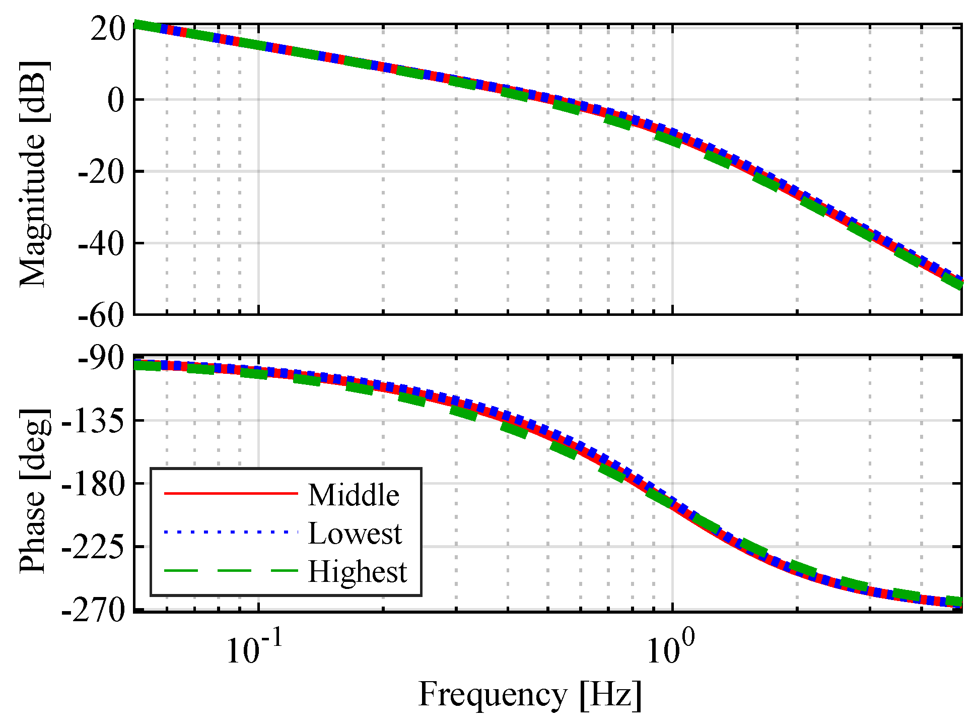
3.2. Resonance and System Damping

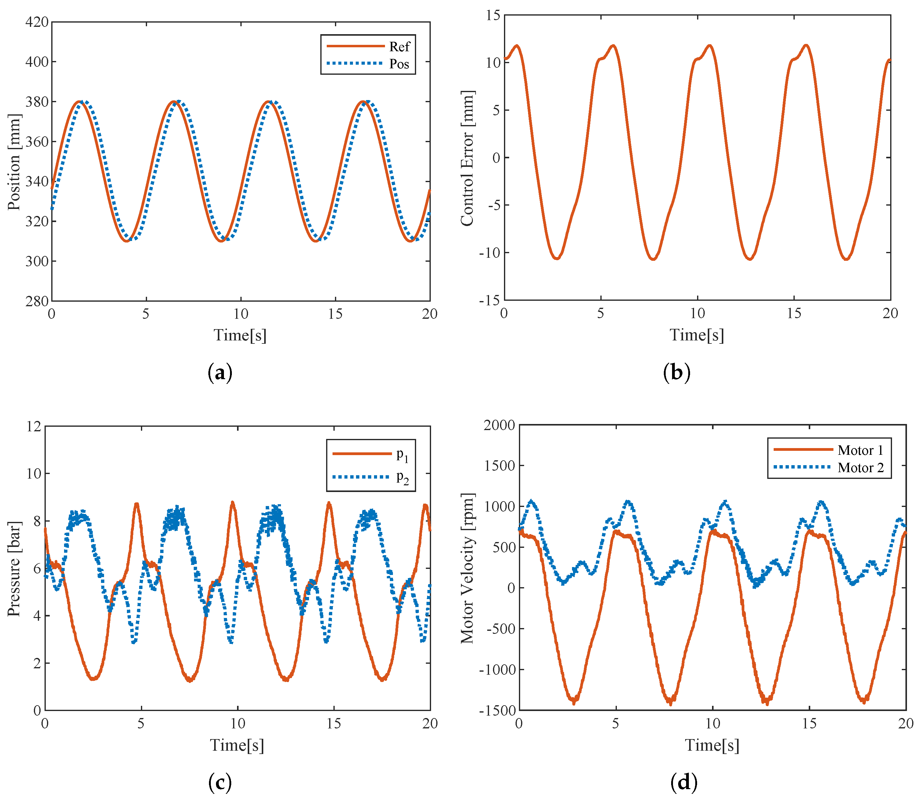
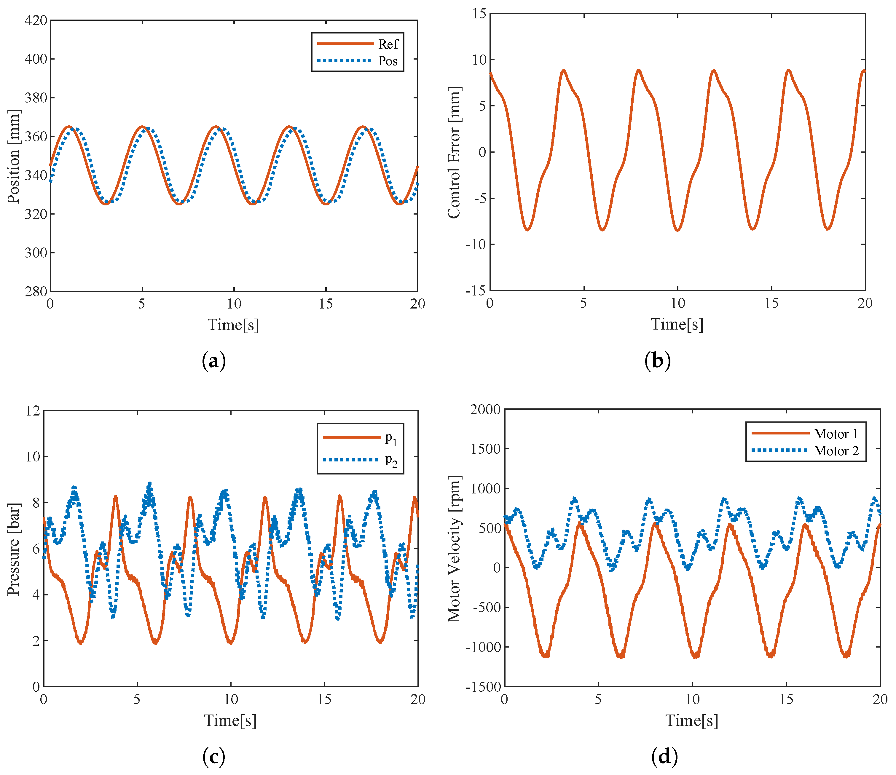
With an effective bulk modulus as low as identified in this paper, one would not expect a traditional valve-controlled cylinder to be able to provide any significant performance under feedback control. This is because the frequency response of valve-controlled cylinders contains a lightly damped resonance, due to the lack of damping in the system. That is, however, not the case for pump-controlled cylinders. Observe from Figure 13 that, for all values of $\beta$, the system’s frequency response is smooth (that is, free of resonant peaks). The reason for this is the presence of adequate damping in the system. With a viscous friction of only $b=100\mathrm{Ns}/\mathrm{m}$, it would be natural to assume that the reason for these smooth responses is solely due to the amount of pump leakage present in the system. That is, however, not the case, as will be demonstrated briefly here.

Figure 14 shows the original frequency response of the system indicated by the solid line (“Original”). Next, the frequency response of the system where the leakage coefficient $c_{12}$ was reduced by a factor of 10 is plotted (with $c_1$ and $c_2$ reduced accordingly), indicated by the dotted line (“reduced leakage”). This could occur either from using a different pump unit with higher leakages or from pump degradation over time. Notice the increased resonant tendency in both the magnitude and phase characteristics of the system. This reveals the inherent property of the system, where the mass, m, the system’s elasticity (influenced by the bulk modulus $\beta$), and the presence of damping essentially function like a mass-spring-damper system. Next, the coupling of the electric drives to the hydraulic pressures (the last terms in (10) and (11)) is eliminated from the model, corresponding to the feedback paths after $G_5$ and $G_6$ in the block diagram of Figure 4. The resulting frequency response is indicated by the dashed line in Figure 14, where the resonant characteristics of the system are now apparent, with a resonant frequency in the vicinity of 0.8 Hz. This demonstrates that damping may be introduced in pump-controlled cylinders via the interaction between the electro- and hydro-mechanical systems, as previously shown by the authors in a numerical study [22].

This demonstrates the importance of using the governing equations of the electric motor when modeling pump-controlled cylinders, as opposed to using first- or second-order approximations (from input to output angular velocity), which are commonly used in the research literature; see [22] for a detailed discussion. In conclusion, due to the presence of pump leakage and the dynamic coupling between the electro- and hydro-mechanical systems, adequate performance under feedback control could be expected from pump-controlled cylinders even with a relatively low effective bulk modulus.

3.3. Feedback Control Design

For assessing the achievable performance under feedback control, a feedback controller must be selected. As shown previously, the system is already adequately damped, with a frequency response characteristic that appears slightly overdamped, so there is no need—nor any benefit—to introducing additional damping into the system via, e.g., acceleration feedback or load pressure feedback, as is commonly done in valve-controlled systems.

In fact, this would likely reduce the achievable performance.

Next, seeing as the system is already type 1 (as evidenced by the phase responses of Figure 13, starting at −90 degrees), there is no need for an integrator in the controller.

For the performance assessment to be conducted in the following, typical frequencies for sinusoidal reference signals of wave compensation platforms (i.e., 0.1 Hz, 0.2 Hz, and 0.25 Hz) will be used. This is fairly close to the 0 dB crossover of the system, and therefore, lag compensation is not going to benefit the tracking accuracy noticeably.

The natural choice from the classical feedback control structures in this case is then either a simple P-controller or a PD/P-Lead. Introducing a D-term or a lead element could theoretically improve the system’s tracking accuracy to some extent; however, the authors are of the opinion that introducing a phase lead near the resonant frequency of a system is not a good practice even if the resonance is adequately dampened. For this reason, a simple P-controller is selected, with $K_p=25$ as utilized in the parameter identification experiments.

Additionally, in order to assess stability for larger strokes in line with the methodology proposed in Section 2.2, as well as assess the performance under feedback control, sinusoidal reference signals of up to $\pm 50\mathrm{mm}$ will be utilized. Unlike the small-stroke step signals (5 mm), this introduces some variations in the effective mass as well as the volumes of the system. Using a Simulink Multibody model of the system, it was found that the effective mass varies from $9958\mathrm{kg}$ to $\mathrm{12,373}\mathrm{kg}$ for $-50\mathrm{mm}$ and $+50\mathrm{mm}$ from mid-stroke, respectively. Additionally, the volumes vary as well, as described by (6) and (7). Figure 15 shows the original frequency response of the system indicated by the dashed line (“Middle”) at mid-stroke, whereas the dotted (“Lowest”) and dashed lines (“Highest”) show the corresponding frequency response at the lowest and highest cylinder positions, respectively, accounting for the mass and volume variations. As can be seen from the figure, the frequency responses are fairly similar, with the PM increasing by 1.4 degrees in the lowest position and the gain margin remaining virtually unchanged. In the highest position, the PM of the system decreases by only 2 degrees with the gain margin increasing slightly. In conclusion, the selected feedback controller of $K_p=25$ is suitable for the entire stroke to be utilized.

3.4. Performance Under Feedback Control

Next, the achievable performance of the pump-controlled cylinder is assessed using sinusoidal reference signals typical of those of wave compensation platforms. By utilizing the feedback controller selected in the previous section, this also allows for verifying large-stroke stability per the methodology presented in Section 2.2. For this purpose, sinusoidal reference signals with frequencies of 0.1 Hz, 0.2 Hz, and 0.25 Hz will be utilized, with an amplitude of $\pm 50\mathrm{mm}$ for the 0.1 Hz signal, $\pm 35\mathrm{mm}$ for the 0.2 Hz signal, and $\pm 20\mathrm{mm}$ for the 0.25 Hz signal.

Figure 16a shows the response of the experimental system (“Pos”) to the 0.1 Hz sinusoidal reference signal (“Ref”), with the control error, pressures, and motor velocities given in Figure 16b–d. As can be seen from the figures, the response of the system is stable and it is able to follow the reference quite closely, with a maximum control error of 8.52 mm. For a wave compensation platform, this would correspond to an 83 percent reduction in the wave amplitude, which is quite decent for such a large inertia.

Next, the system’s response to the 0.2 Hz sinusoidal reference signal is given by Figure 17, where it may be seen that the system is able to track the reference quite well. The maximum control error is 11.8 mm, corresponding to a 66 percent reduction in the wave amplitude for a wave compensation platform. Observe from Figure 17d that despite utilizing a significantly larger portion of the pump’s velocity range compared to the identification data, the system remains stable. This serves as a validation of the control design and analysis methodology presented in Section 2.2.

Lastly, the system’s response to the 0.25 Hz sinusoidal reference signal is given by Figure 18, where the maximum control error is 8.82 mm, corresponding to a wave reduction of 56 percent. In general, the performance of the system for all reference signals is quite adequate, especially considering the large inertia load.

4. Discussion

The minimum occurring value of the effective bulk modulus for the pump-controlled cylinder studied here has been identified as 165 bar. This is in contrast to traditional valve-controlled systems, where values above 6000 bar may normally be assumed with confidence. For a valve-controlled system controlling a large inertia load of this magnitude (above 10,000 kg), adequate performance under feedback control would certainly not have been achievable. This is, however, not the case for the pump-controlled system studied here, where adequate performance was in fact achieved despite this extremely low effective bulk modulus. As seen in Figure 6, a swift response is observed for the system, with a rise time of approximately 0.36 s. Furthermore, for tracking of sinusoidal references, adequate tracking accuracy was found for frequencies representative of real-life wave compensation platforms. This is quite significant and certainly not an intuitive result considering the approximately forty-fold reduction in the effective bulk modulus relative to valve-controlled systems, and is due to the presence of adequate damping. For valve-controlled systems, the only sources of damping are due to valve leakage and cylinder friction, which are normally quite low, with damping ratios as low as 0.1 and 0.2 being quite common in practice [3]. As demonstrated in Section 3, however, damping in the pump-controlled cylinder may be provided not just from actuator friction and pump leakage, but also due to an internal feedback path coupling the dynamics of the electric motors and the hydro-mechanical system. This emphasizes the importance of correct modeling of these systems, as this internal coupling is not captured by the previously described modeling approximations commonly used in the literature.

Based on the results presented here, it may be concluded that adequate performance under feedback control may be achieved using low-pressure pump-controlled cylinders in some applications, even for large inertia loads. This will, however, not always be the case, and the outcome depends both on the mechanical properties of the system (effective inertia and external load conditions) as well as the amount of undissolved air in the fluid. The results presented here for a single system apply to pump-controlled cylinders in general, in a broader sense, but with some restrictions. In particular, the amount of undissolved air present in the system is going to vary from one experimental application to another. This aspect of hydraulic control systems may be highly uncertain, and reference values should be taken only as approximations. The results and reference values presented here, however, may serve as references and guidelines for future applications. Having an established reference value for the effective bulk modulus of low-pressure pump-controlled cylinders is of value not just for the analysis and design of feedback controllers, but also for system design and circuit selection, as will be made clear in the following.

Whether or not a low-pressure pump-controlled cylinder will be able to achieve adequate performance will vary from application to application. Having established reference values for the minimal effective bulk modulus and pump leakages, this may be predicted for a given application using LTI models with some degree of accuracy prior to the system’s construction. For applications where such estimates indicate the suitability of a low-pressure pump-controlled cylinder with high certainty, their use in feedback control applications may certainly be recommended. If predictions based on LTI models using reference values indicate uncertainty, however, the use of alternative hydraulic circuits capable of providing a higher effective bulk modulus is certainly recommended.

Lastly, for the modeling of pump-controlled systems, attention is brought to two critical factors. First, the internal feedback that couples the dynamics of the electro- and hydro-mechanical systems, which was first pointed out by the authors in a numerical study in [22]. As can be seen from Figure 14, this internal feedback has the potential to provide significant contributions to the overall damping of the system. Its damping effect will not be included in an LTI model if the dynamics of the electric drive are simplified to that of a first- or second-order transfer function, as is commonly done in the research literature. This could result in both significant model mismatches as well as incorrect parameter estimations, which could lead to poorly designed feedback controllers. Secondly, the pronounced effects of the velocity feedforward on the electric drive on the overall dynamics of the system were demonstrated, as evidenced by Figure 11. To the best of the authors’ knowledge, this has not yet been addressed in the research literature, and such feedforwards are found today on most commercially available electric drives. As with the internal coupling between the electro- and hydro-mechanical systems, failure to model this critical aspect of a pump-controlled cylinder could lead to both significant model errors and incorrect parameter estimations, as well as poorly designed feedback controllers.

5. Conclusions

In this paper, the effective bulk modulus of low-pressure pump-controlled cylinders has been investigated. Using an experimental test rig, the minimal occurring effective bulk modulus of a pump-controlled cylinder was identified as 165 bar for a system controlling a large inertia load with an effective mass greater than 10,000 kg. The impact of having such a low effective bulk modulus on the achievable performance was studied using frequency domain analysis. It was demonstrated that despite this drastic reduction in the effective bulk modulus relative to traditional valve-controlled systems, adequate performance could be achieved in this application, even for a large inertia load, due to the presence of adequate damping. This may, however, not always be the case, and caution is advised regarding the use of these systems in applications where feedback control is required. For this purpose, recommendations have been given that may serve as guidelines, along with the reference values established here, for future applications where low-pressure, pump-controlled cylinders are considered in feedback control systems. Additionally, critical modeling aspects of these systems that are commonly neglected in the literature have been identified, and their importance has been demonstrated. Lastly, a methodology for designing feedback controllers for pump-controlled cylinders—based on a single worst-case operating point, analogous to that traditionally used for valve-controlled cylinders—has been proposed and validated.

References

- Michel, S.; Weber, J. Electrohydraulic Compact-drives for Low Power Applications considering Energy-efficiency and High Inertial Loads. In Proceedings of the 7th FPNI PhD Symposium on Fluid Power, Reggio Emilia, Italy, 27–30 June 2012; pp. 1–18. [Google Scholar]
- Michel, S.; Weber, J. Energy-efficient electrohydraulic compact drives for low power applications. In Proceedings of the ASME/BATH, Bath, UK, 12–14 September 2012; pp. 12–14. [Google Scholar]
- Merritt, H.E. Hydraulic Control Systems; John Wiley and Sons: New York, NY, USA, 1967. [Google Scholar]
- Manring, N.D.; Fales, R.C. Hydraulic Control Systems; John Wiley and Sons: New York, NY, USA, 2019. [Google Scholar]
- Long, Q.; Neubert, T.; Helduser, S. Principle to closed loop control differential cylinder with double speed variable pumps and single loop control signal. In Proceedings of the Fourth International Symposium on Fluid Power Transmission and Control (ISPP’ 2003), Wuhan, China, 28 August 2003. [Google Scholar]
- Padovani, D.; Ketelsen, S.; Hagen, D.; Schmidt, L. A self-contained electro-hydraulic cylinder with passive load-holding capability. Energies 2019, 12, 292. [Google Scholar] [CrossRef]
- Jarf, A.; Minav, T.; Pietola, M. Nonsymmetrical flow compensation using hydraulic accumulator in direct driven differential cylinder application. In Proceedings of the 9th FPNI PhD Symposium on Fluid Power, Florianópolis, Brazil, 26–28 October 2016; Volume 50473. [Google Scholar]
- Goytil, P.H.; Padovani, D. Motion control of large inertia loads using electrohydrostatic actuation. In Proceedings of the 2020 IEEE 16th International Workshop on Advanced Motion Control (AMC), Kristiansand, Norway, 14–16 September 2020; IEEE: Piscataway, NJ, USA, 2020; pp. 73–78. [Google Scholar]
- Hagen, D.; Padovani, D.; Choux, M. A Comparison Study of a Novel Self-Contained Electro-Hydraulic Cylinder Versus a Conventional Valve-Controlled Actuator—Part 1: Motion Control. Actuators 2019, 8, 79. [Google Scholar] [CrossRef]
- Long, Q.; Neubert, T.; Helduser, S. Differential cylinder servo system based on speed variable pump and sum pressure control principle. In Proceedings of the Fifth International Conference on Fluid Power Transmission and Control, Hangzhou, China, 3–5 April 2001; pp. 69–73. [Google Scholar]
- Gholizadeh, H.; Burton, R.; Schoenau, G. Fluid bulk modulus: Comparison of low pressure models. Int. J. Fluid Power 2012, 13, 7–16. [Google Scholar] [CrossRef]
- Goytil, P.H.; Padovani, D.; Hansen, M.R. A novel solution for the elimination of mode switching in pump-controlled single-rod cylinders. Actuators 2020, 9, 20. [Google Scholar] [CrossRef]
- Mommers, R.; Achten, P.; Achten, J.; Potma, J. Benchmarking the performance of hydrostatic pumps. In Proceedings of the 17th Scandinavian International Conference on Fluid Power, Linköping, Sweden, 1–2 June 2021; pp. 322–331. [Google Scholar]
- Ellis, G. Control System Design Guide: Using Your Computer to Understand and Diagnose Feedback Controllers; Butterworth-Heinemann: Oxford, UK, 2012. [Google Scholar]
- Goytil, P.H.; Padovani, D.; Hansen, M.R. On the energy efficiency of dual prime mover pump-controlled hydraulic cylinders. In Proceedings of the ASME/BATH 2019 Symposium on Fluid Power and Motion Control, Longboat Key, FL, USA, 7–9 October 2019; Volume 59339. [Google Scholar]
- Ketelsen, S.; Andersen, T.O.; Ebbesen, M.K.; Schmidt, L. A self-contained cylinder drive with indirectly controlled hydraulic lock. Model. Identif. Control 2020, 41, 185–205. [Google Scholar] [CrossRef]
- Caliskan, H.; Balkan, T.; Platin, B.E. Hydraulic position control system with variable speed pump. In Proceedings of the ASME 2009 Dynamic Systems and Control Conference, Hollywood, CA, USA, 12–14 October 2009; Volume 48920, pp. 275–282. [Google Scholar]
- Boes, C.; Helbig, A. Electro hydrostatic actuators for industrial applications. In Proceedings of the 9th International Fluid Power Conference, Aachen, Germany, 24–26 March 2014; pp. 134–142. [Google Scholar]
- Hagen, D.; Padovani, D.; Ebbesen, M.K. Study of a self-contained electro-hydraulic cylinder drive. In Proceedings of the 2018 Global Fluid Power Society PhD Symposium (GFPS), Samara, Russia, 8–20 July 2018; IEEE: Piscataway, NJ, USA, 2018; pp. 1–7. [Google Scholar]
- Zhao, W.; Bhola, M.; Ebbesen, M.K.; Andersen, T.O. A Novel Control Design for Realizing Passive Load-Holding Function on a Two-Motor-Two-Pump Motor-Controlled Hydraulic Cylinder. Model. Identif. Control 2023, 44, 125–139. [Google Scholar] [CrossRef]
- Costa, G.; Sepehri, N. Hydrostatic Transmissions and Actuators: Operation, Modelling and Applications; John Wiley and Sons: New York, NY, USA, 2015. [Google Scholar]
- Goytil, P.H.; Padovani, D.; Hansen, M.R. Linear Time-Invariant Modelling of Electrohydraulic Cylinders. In Proceedings of the 2022 International Conference on Electrical, Computer, Communications and Mechatronics Engineering (ICECCME), Maldives, 16–18 November 2022; IEEE: Piscataway, NJ, USA, 2022; pp. 1–6. [Google Scholar]