Precise Control of Following Motion Under Perturbed Gap Flow Field

Abstract

The control of following motion under mesoscale gap flow fields has important applications. The flexible characteristics of the plant, wideband time-varying disturbances caused by the flow field, and requirements of high precision and low overshoot make achieving submicron level accuracy a significant challenge for traditional control methods. This study adopts the control concept of Disturbance Observer Control (DOBC) and uses H_∞ mixed-sensitivity shaping technology to design a Q-filter. Simultaneously, multiple control techniques, such as high-order reference trajectory planning, Proportional-Integral-Derivative (PID) control, low-pass filtering, notch filtering, lead lag correction, and disturbance rejection filtering, are applied to obtain a control system with a high open-loop gain, sufficient phase margin, and stable closed-loop system. Compared to traditional control methods, the new method can increase the open-loop gain by 15 times and the open-loop bandwidth by 8%. We even observed a 150-time increase of the open-loop gain at the peak frequency. Ultimately, the method achieves submicron level accuracy, making important advances in solving the control problem of semiconductor equipment.

1. Introduction

Gap flow fields play an important role in industrial equipment. For example, gap flow fields are essential for liquid or gas dynamic bearings to achieve force bearing [1,2]. In hydraulic pumps, gap flow fields help lubricate surfaces and reduce vibrations between the plunger and the cylinder body [3]. Furthermore, hydraulic conveying systems for cylinder loading pipelines provide conveying power through annular gap flow fields [4]. In the semiconductor equipment, a mesoscale gap flow field needs to be maintained between two moving parts A and B, with part A located above part B. Both part A and part B can achieve horizontal and vertical motion, and part A needs to follow B in vertical direction to maintain the parallel gap. The gap is less than 0.1 mm, and the surface microstructure of the moving parts is mesoscopic. With fluid structure coupling, the mesoscale gap flow field generates complex disturbance forces, which can be divided into micro-tube gas-liquid two-phase flow disturbance [5,6,7,8,9], Rayleigh step disturbance [10,11,12], and squeeze film disturbance based on their forming mechanisms [13,14]. This work manifests the disturbance force of the mesoscale gap flow field as a wideband time-varying disturbance.

Existing research has proposed a series of methods for motion control under time-varying disturbances, including Active Disturbance Rejection Control (ADRC), which is used for uncertain systems [15,16], adaptive control, which automatically adjusts controller parameters [17], and Disturbance Observer Control (DOBC), which is widely used owing to its simplicity, effectiveness, and excellent disturbance suppression effect [18,19]. Yang et al. addressed the dynamic coupling vibration problem of high-speed macro–micro robotic arms [20]. By improving discrete sliding mode control and designing a variable speed approach law to adjust the sliding mode switching gain, high-frequency chattering was suppressed. Simultaneously, adaptive laws were used to compensate for parameter perturbations and external disturbances online, and tracking errors were controlled at the micrometer level. Smith et al. addressed the robust control problem of small fixed-wing unmanned aerial vehicles under complex disturbances [21]. They used a disturbance observer to estimate external wind disturbances, model uncertainties, and other composite disturbances in real time. Combined with anti-saturation mechanisms such as integral limiting or dynamic compensation, this approach suppressed the integral accumulation problem caused by actuator saturation, thereby improving the robustness of the system. In the scenario of sudden wind disturbances and load changes, the joint DOBC and anti-saturation reduced the attitude angle tracking error by 60%.

As mentioned above, submicron precision following motion control of two moving components under wideband time-varying disturbances presents significant engineering implementation challenges. First, the moving parts that control the gap flow field are not ideal rigid structures and have flexible characteristics, which can lead to a gain decrease in the low-frequency band and resonance peaks in the mid-to-high frequency bands. Second, owing to the wideband time-varying disturbance and the disturbance frequency band covering the mechanical modal frequency band of the system, the accuracy easily deteriorates. Finally, in the following motion control scenario, high response speed, small tracking error, and low overshoot are required in order to avoid collision. The system thus needs to have both a high open-loop gain and sufficient phase margin, which is difficult to achieve when the system is flexible and delayed. Traditional control methods cannot address the challenges caused by plant characteristics, external disturbance characteristics, and control performance requirements.

This study adopts the DOBC control concept and uses H_∞ mixed-sensitivity shaping technology to design a Q-filter. Simultaneously, multiple control techniques, such as high-order reference trajectory planning, PID control, low-pass filtering, notch filtering, lead lag correction, and disturbance rejection filtering are comprehensively applied to obtain a stable closed-loop control system with a high open-loop gain and sufficient phase margin.

This method contributes a few innovations.

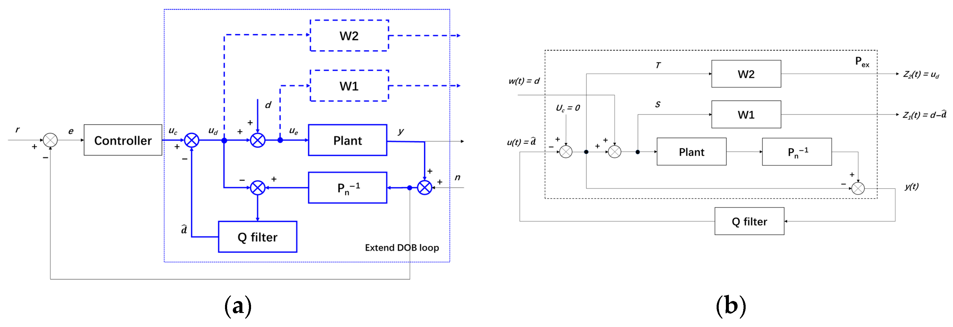
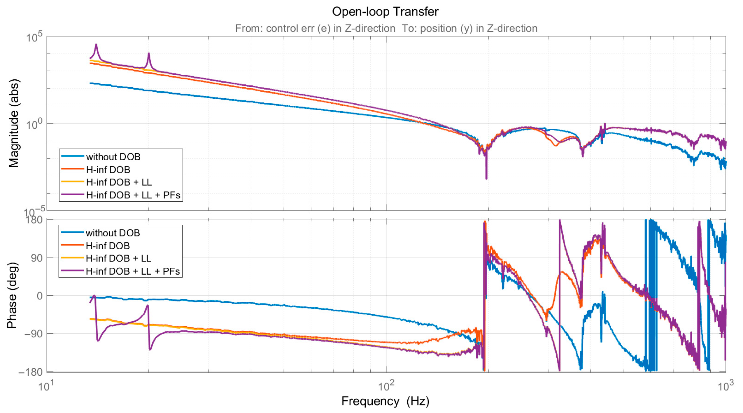
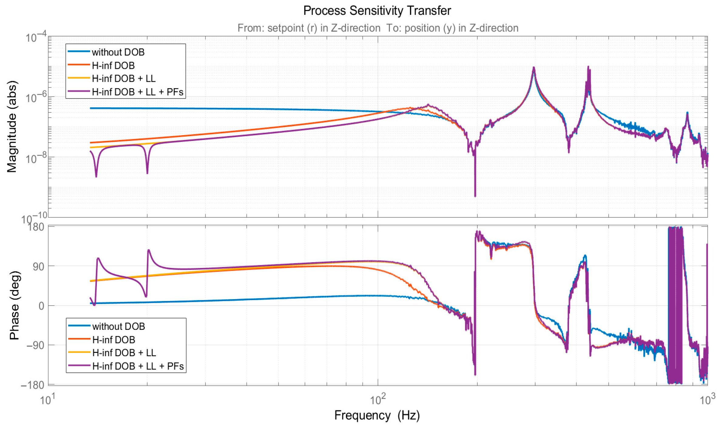
• Decoupling the Disturbance Observer (DOB) loop from the outer control loop, the method constructs extended DOB loop with zero output from the outer control loop. Then, it uses H_∞ mixed-sensitivity shaping technology to design a Q-filter. The H_∞ DOBC is used for the overall suppression of wideband time-varying disturbances, significantly increasing the open-loop gain in the low-frequency range and enhancing the phase margin.
• The method combines DOBC with lead lag correction, which improves the open-loop gain in the low to mid frequency range, compensating for the open-loop gain loss in the mid frequency range introduced by the H_∞ DOBC.
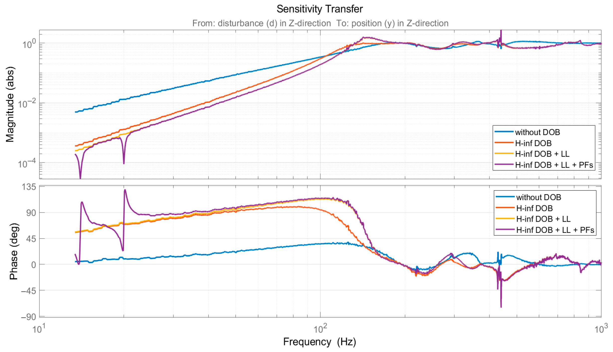
• Disturbance rejection filtering correction is used to suppress certain concentrated frequency bands in the flow field disturbances and improve the open-loop gain.

Ultimately, the system achieves submicron level accuracy.

Table 1. Comparison between traditional control method and the H_∞ DOBC method.

Challenges	Traditional Methods	This H∞ DOBC Method
Special plant characteristics, such as flexibility, multimodality, system delay and so on	Gain decrease in the low-frequency band and resonance peaks in the mid-to-high frequency bands	High open-loop gain in the low-frequency band and no resonance peaks
Wideband time-varying external disturbance	Large disturbance sensitivity	Small disturbance sensitivity over a wide frequency range, and extremely small disturbance sensitivity in peak frequency
Special control requirements	Cannot simultaneously achieve high open-loop gain and large phase margin	Simultaneously achieve high open-loop gain and sufficient phase margin

compares this H_∞ DOBC method with traditional methods.

2. Materials and Methods

The motion control of both part A and part B is multi-input and multi-output (MIMO). To study motion control under wideband time-varying disturbances, we decouple MIMO into a series of single inputs and single outputs (SISO). This article describes the controller design method for SISO in the Z direction of part A. The software used for control system simulation and data processing in this study is MATLAB R2023a.

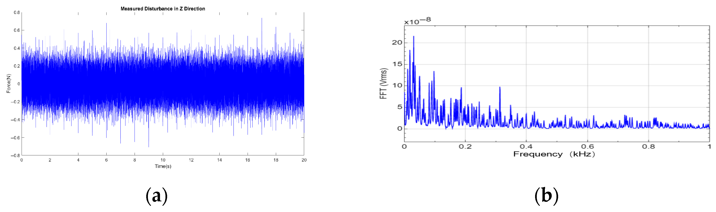
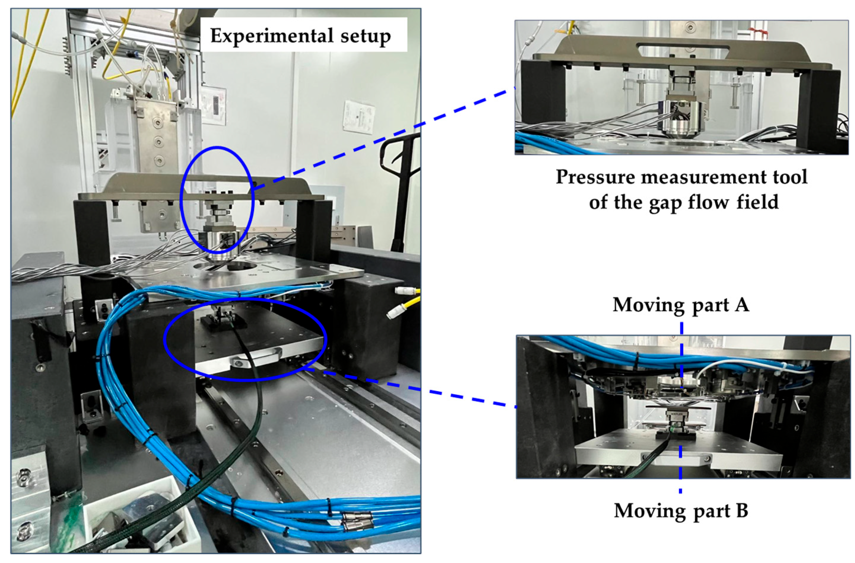
2.1. Disturbance Force Measurement

As a preliminary step, we first used a force-measuring tool (customized devices, Hangzhou, China) to measure the disturbance force of the gap flow field between part A and the flat plate of the tool, as shown in Figure 1b. During measurement, component A was stationary while the flow field was flowing. The measurement band of sensors (HBM U9C, Darmstadt, Germany) was 1.2 kHz, and the sampling frequency was 10 kHz. The results showed that a wideband time-varying disturbance was caused by the mesoscale gap flow field, as presented in Figure 2. The frequency band of disturbance force covered frequences 0~1000 Hz and above, but mainly concentrated in 0~400 Hz. The peak frequency and amplitude exhibited time-varying characteristics.

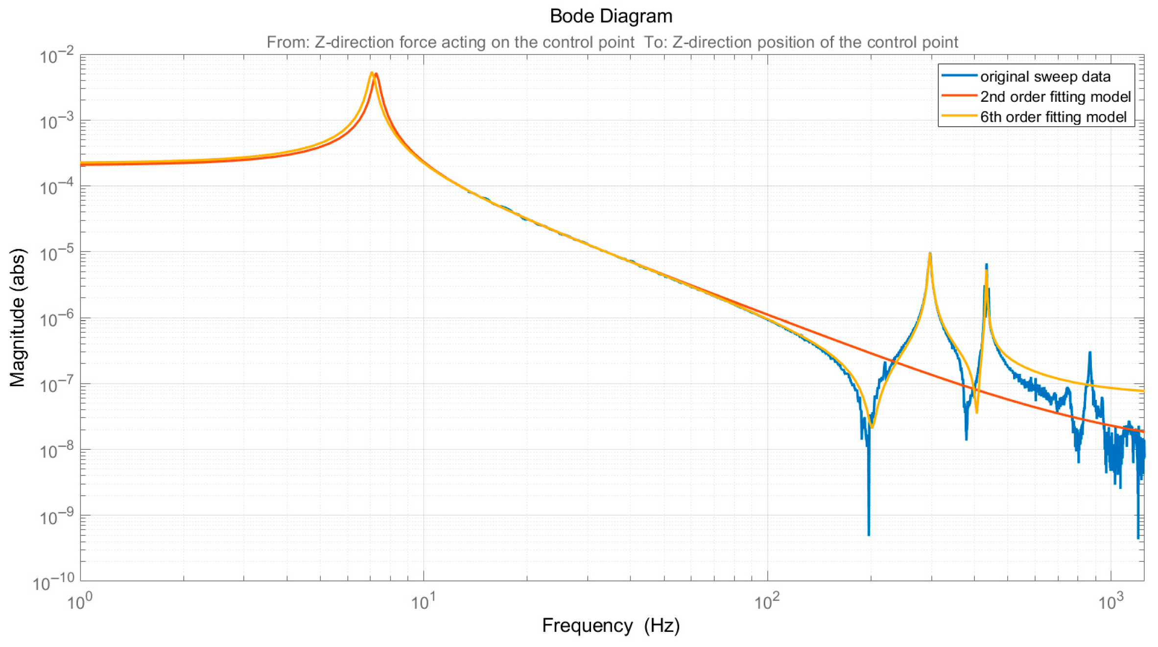
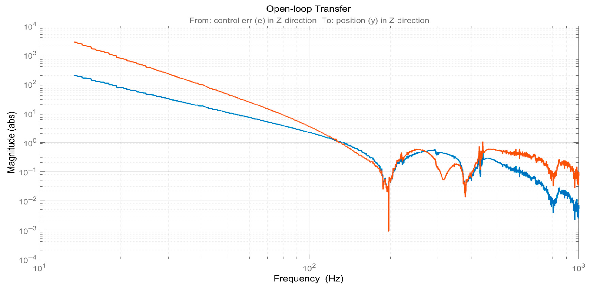
2.2. Plant Identification

This study examines plants as a fully linear time-invariant system. Because wideband time-varying disturbances are mainly concentrated in the low-to-mid frequency band, it is necessary to accurately model the system transfer function in this frequency band, including the flexible multimodal characteristics of the plant. Using the exponential sine sweep method [22], we obtained the raw sweep-response data under nonstationary interference conditions. The raw sweep-response data were fitted with a continuous transfer function model using nonlinear least-squares methods [23]. As shown in Figure 3, the blue curve represents the original sweep frequency response data, the yellow curve represents the fitting of a 2nd-order Spring-Mass-Damper (SMD) model, and the red curve represents the fitting of a sixth-order model including one 2nd-order SMD model and two 2nd-order modal models. Equation (1) shows the fitted continuous model, which is a combination of one SMD 2nd-order model and multiple 2nd-order modal models. The fitting results were consistent with the modal testing results of the hammering method. Part A had structural modal frequencies of 297 Hz and 434 Hz and flexible connection modal frequency of 7.14 Hz.

$$Plant\left(s\right)={\displaystyle \frac{1}{M{s}^2+Cs+K}}+\sum _{j=1}^n{\displaystyle \frac{k_j}{s^2+2{\xi }_j{\omega }_{j}s+{{\omega }_j}^2}}$$

(1)

In Equation (1), $Plant\left(s\right)$ represents the mechanical transfer function of the plant, $M$ represents the mass of the plant, $C$ represents the damping of the plant, $K$ represents the stiffness of the plant, ${\omega }_j$ represents the $j$-th modal frequency of the plant, and ${\xi }_j$ and $k_j$ represent the $j$-th modal parameters of the plant.

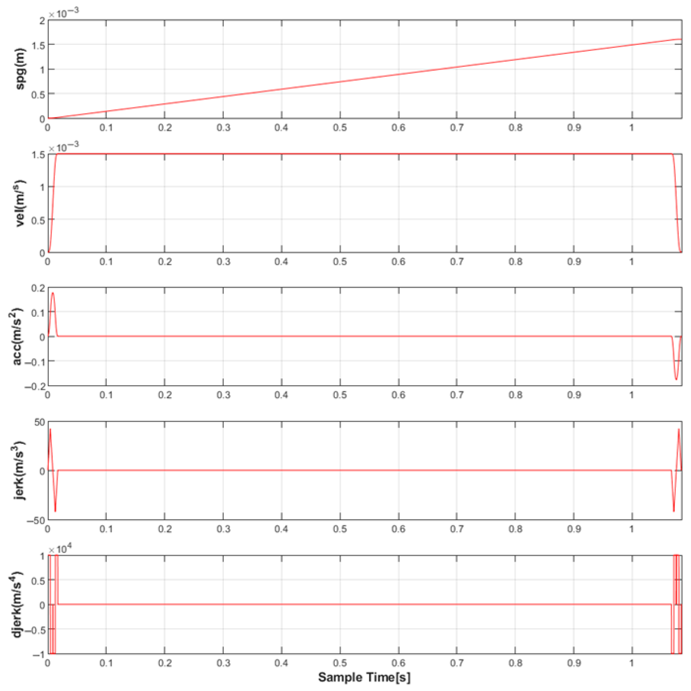
2.3. High-Order Reference Trajectory Planning

In the following motion control of mesoscale gap flow fields, to avoid collisions caused by excessive overshoot due to direct input of step signals, a fourth-order trajectory planning algorithm is used to ensure that the trajectory is continuous in position, velocity, acceleration, jerk, and djerk [24]. The trajectory is composed of segmented fifth-order polynomials, and the time interval of each trajectory segment is [$t_k$, $t_{k+1}$], as shown in Equation (2):

$$p\left(t\right)=\sum _{j=0}^4{\alpha }_j{(t-t_k)}^j$$

(2)

In Equation (2), $j$ represents the polynomial order, and ${\alpha }_j$ represents the position, velocity, acceleration, jerk, and djerk of the time domain class [$t_k$, $t_{k+1}$], which are solved through boundary conditions such as starting and ending point positions, maximum velocity, maximum acceleration, and maximum jerk.

2.4. DOBC Design

To solve the control problem caused by wideband time-varying disturbances and its frequency band covering the mechanical modal frequency band of the system, our method uses the DOB to estimate disturbances and system uncertainties and feed the estimation values back to the forward channel of the control system. As shown in Figure 4, the dashed box shows the DOB loop, which consists of a nominal object inverse model ${P_n}^{-1}$ and a Q-filter. The other parts are the outer control loop, where r is the reference input, y is the measurement output, d is the external disturbance, $\widehat{d}$ is the disturbance evaluation value, n is the measurement noise, e is the control error, u_c is the controller output, u_d is the DOB control input, and u_e is the plant input.

The core idea of DOB is to treat the difference between the actual output of the controlled object and the nominal model output as equivalent interference, and compensate it to the input end to eliminate the influence of external interference. The system performance of the frequency-domain DOB largely depends on the selection of the cutoff frequency of the Q-filter, and due to the existence of phase lag, the results have a certain degree of conservatism [19]. In order to meet the requirements of following motion control in mesoscale gap flow fields, while achieving high open-loop gain and large phase margin, this study uses the H_∞ mixed-sensitivity shaping technique to design a Q-filter [25], and uses a nonlinear least-squares method to fit the Q-filter to achieve reduced order design, ensuring system stability [23]. 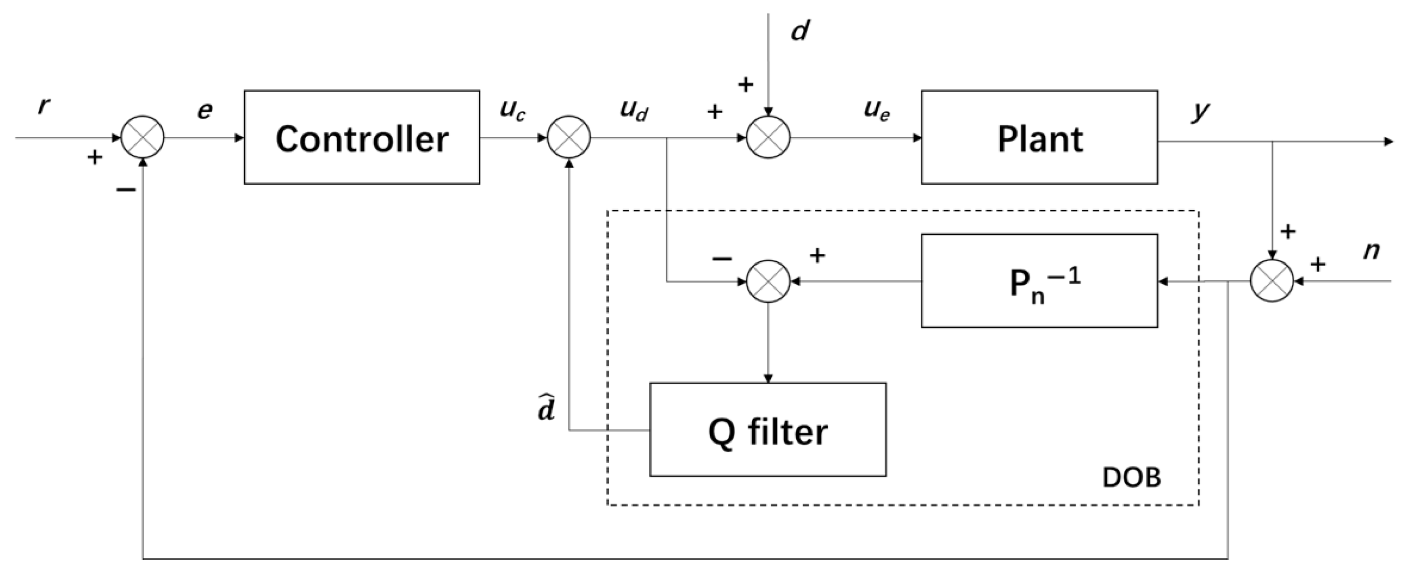Because DOB does not change the stability of the closed-loop transfer function of the original system, the DOB loop and the outer control loop can be decoupled in design.

2.4.1. Outer Control Loop Design

The core of the outer control loop is the controller. An integral saturated PID controller is used for the closed loop based on position feedback, and its continuous transfer function is given by Equation (3). The parameters of PID are determined based on designed open-loop bandwidth and empirical formulas.

$$PID\left(s\right)=P{\displaystyle \frac{\left(1+ND\right)s^2+\left(N+I\right)s+NI}{s^2+Ns}}$$

(3)

Here, P represents the proportional coefficient, I represents the integral coefficient, D represents the differential coefficient, and N represents the length of the sampling data per second.

A low-pass filter is used to filter the PID controller output to suppress the influence of sensor noise. The setting of the filter parameters should take into account the frequency band of wideband time-varying disturbances, measurement noise frequency band, and frequency band of the reference input. The continuous transfer function is given by Equation (4):

$$LPF\left(s\right)={\displaystyle \frac{{{\omega }_l}^2}{s^2+2{\xi }_l{\omega }_{l}s+{{\omega }_l}^2}}$$

(4)

Here, ${\omega }_l$ represents the cutoff frequency of the low-pass filter, and ${\xi }_l$ represents the damping ratio of the low-pass filter.

Finally, notch filtering is used to suppress the multimodal effects of the plant. The filter parameters are set based on the modal characteristics of each order in the sweep-response data. The continuous transfer function is given by Equation (5). The parameters of notch filters are determined based on mechanical transfer function test results.

$$Notchs\left(s\right)=\prod _{j=1}^k{\displaystyle \frac{s^2+2{\xi }_{nzj}{\omega }_{nj}s+{{\omega }_{nj}}^2}{s^2+2{\xi }_{npj}{\omega }_{nj}s+{{\omega }_{nj}}^2}}$$

(5)

Here, ${\omega }_{nj}$ represents the center frequency of the $j$-th notch filter, and ${\xi }_{nzj}$ and ${\xi }_{npj}$ represent the damping coefficients of the control zeros and poles of the $j$-th notch filter, respectively, which are determined by the notch width and depth.

2.4.2. DOB Loop Design

The design of the DOB loop mainly includes the nominal object inverse model and Q-filter. Owing to the use of notch filters in the design of the outer control loop, only the 2nd-order SMD model in Section 2.1 is used as the nominal object model, disregarding the other parts of the fitting result. The nominal object inverse model is given by Equation (6).

$${P_n}^{-1}\left(s\right)=M{s}^2+Cs+K$$

(6)

Here, $M$ represents the mass of the plant, $C$ represents the damping of the plant, $K$ represents the stiffness of the plant.

The design steps of Q-filter are as follows:

• Based on the DOBC control architecture, the standard H_∞ model for the Q-filter is constructed.
• Mixed-sensitivity weight functions are constructed based on disturbance evaluation error sensitivity and disturbance evaluation compensation sensitivity.
• Based on the H_∞ model, the generalized plant is constructed.
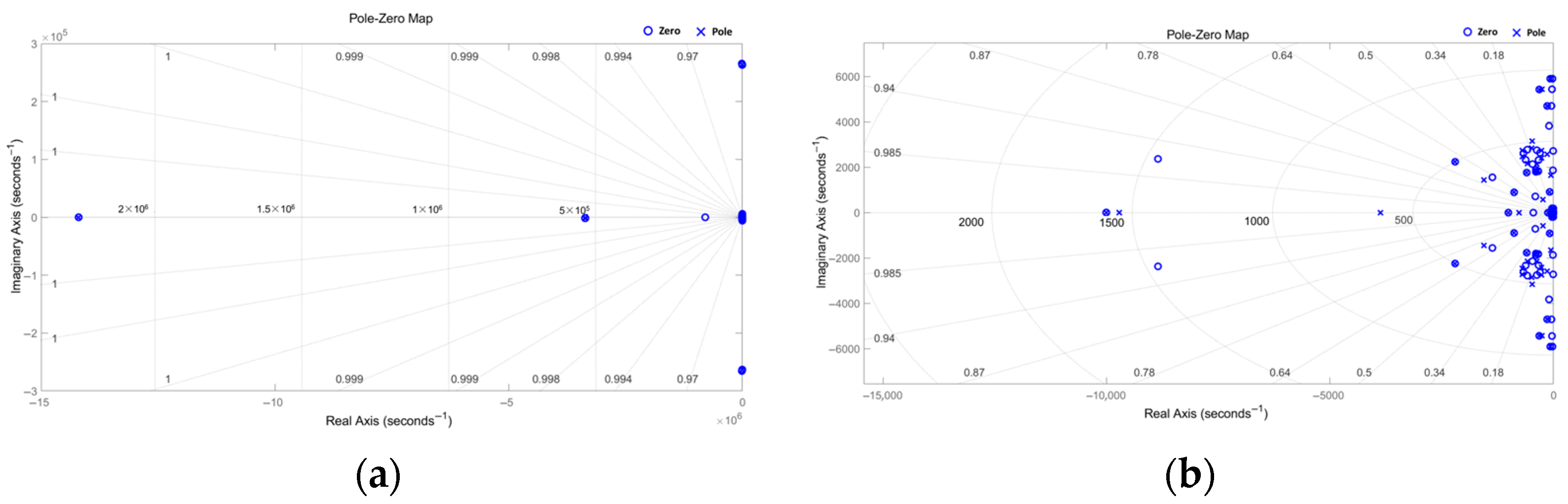
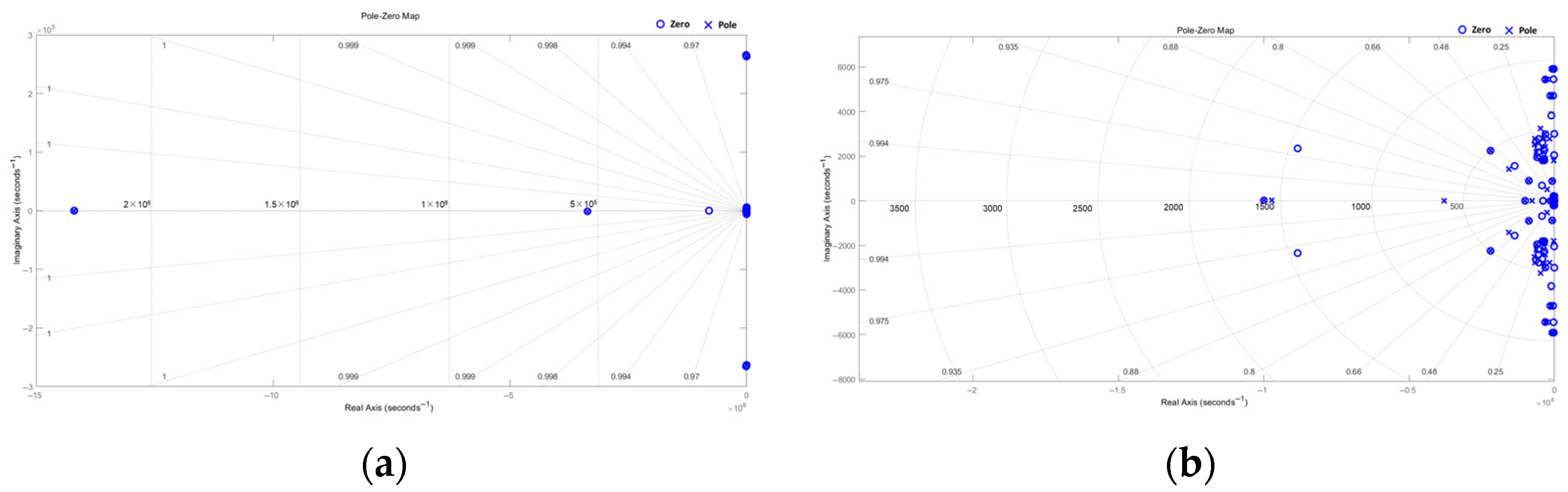
• The H_∞ model is used to solve the Q-filter;
• The nonlinear least squares method is applied to perform order reduction on the Q-filter.

A.

The standard H_∞ model is constructed for the Q-filter

Based on the DOBC control architecture shown in Figure 4, when the output of the outer control loop is zero, the extended DOB loop is equivalent to a generalized plant. As shown in Figure 5a, the blue solid line indicates the DOB and plant in Figure 4, and the blue dashed box indicates the expanded mixed-sensitivity evaluation part. As shown in Figure 5b, the content of the dashed box is the generalized plant P_ex, Plant is the ideal model of the plant, and ${P_n}^{-1}$ is the nominal object inverse model used to construct the Q-filter. u (t), w (t), y (t), z₁ (t), and z₂ (t), respectively, represent the disturbance input, control input, measurement output, tuned output 1, and tuned output 2 of the standard H_∞ model. In particular, u (t) equals the disturbance evaluation value $\widehat{d}$, w (t) equals the external disturbance d, z₁ (t) equals the disturbance evaluation error d-$\widehat{d}$, and z₂ (t) equals u_d. The Q-filter design problem is therefore transformed into solving the H_∞ controller problem for generalized plants [26]: designing the Q-filter to minimize the H_∞ norm of the closed-loop transfer function from the disturbance input w (t) to the tuned outputs z₁ (t) and z₂ (t). In other words, the following equations hold:

$$\begin{gathered} {‖S{W}_1‖}_{\infty }\le {\gamma }_1 \\ {‖T{W}_2‖}_{\infty }\le {\gamma }_2 \end{gathered}$$

(7)

Here, S represents the sensitivity of the disturbance evaluation error, T represents the compensation sensitivity of the disturbance evaluation, W₁ represents the weight function of S, and W₂ represents the weight function of T; constants ${\gamma }_1$ and ${\gamma }_2$ are rational numbers.

B.

Constructing the mixed-sensitivity weight functions

This study uses mixed-sensitivity shaping technology to construct mixed-sensitivity weight functions. As shown in Equation (8), W₁ represents the weight function of the sensitivity of the disturbance evaluation error. Because wideband time-varying disturbances are mainly concentrated in the low-to-mid frequency bands, 1/W₁ is designed as a low-pass filter, and its parameters should consider the frequency band of wideband time-varying disturbances. As shown in Equation (9), W₂ represents the weight function of the compensation sensitivity of the disturbance evaluation, whose robustness must be evaluated in high frequency band. Correspondingly, 1/W₂ is designed as a high-pass filter, and its parameters should take into account the frequency band of wideband time-varying disturbances, too. The continuous transfer functions for W₁ and W₂ are given by Equations (8) and (9):

$$W_1\left(s\right)={\displaystyle \frac{(\frac{1}{{10}^{M_1/20}})s+{\omega }_1}{s+{10}^{M_2/20}{\omega }_1}}$$

(8)

$$W_2\left(s\right)={\displaystyle \frac{s+(\frac{1}{{10}^{M_3/20}}){\omega }_2}{{10}^{M_4/20}s+{\omega }_2}}$$

(9)

Here, ${\omega }_1$ represents the low-pass cut-off frequency of 1/W₁, ${\omega }_2$ represents the high pass cut-off frequency of 1/W₂, M₁ represents the amplitude of the low-frequency band of 1/W₁, M₂ represents the amplitude of the high-frequency band of 1/W₁, M₃ represents the amplitude of the low-frequency band of 1/W₂, M₄ represents the amplitude of the high-frequency band of 1/W₂, and M₁, M₂, M₃, and M₄ are all in decibels.

C.

Constructing the generalized plant

Based on the solution model shown in Figure 5b, the transfer function matrix of the generalized plant can then be constructed as shown in Equation (10), satisfying the requirements shown in Equation (11):

$$P_{ex}\left(s\right)=\left[\begin{array}{cc}{W}_1& -W_1\\ 0& -W_2\\ Plant{P_n}^{-1}& 1-Plant{P_n}^{-1}\end{array}\right]$$

(10)

$$\left[\begin{array}{c}{Z}_1\left(s\right)\\ Z_2\left(s\right)\\ Y\left(s\right)\end{array}\right]=P_{ex}(s)\left[\begin{array}{c}W\left(s\right)\\ U\left(s\right)\end{array}\right]$$

(11)

In the above equations, $Z_1\left(s\right)$, $Z_2\left(s\right)$, $Y\left(s\right)$, $W\left(s\right)$, and $U\left(s\right)$ are the s-domain expressions of the disturbance evaluation error z₁ (t), disturbance evaluation value z₂ (t), measurement output y (t), disturbance input w (t), and control input u (t) in the solution model shown in Figure 5b. $W_1\left(s\right)$, $W_2\left(s\right)$, $Plant\left(s\right)$, and ${P_n}^{-1}\left(s\right)$ are, respectively, the transfer function of the disturbance evaluation error sensitivity, the transfer function of the disturbance evaluation value compensation sensitivity, the transfer function of the fitting object mechanical, and the transfer function of the nominal object inverse model.

D.

Solving the Q-filter

By solving the Riccati equations [27], a controller is found that minimizes the H_∞ norm of the transfer function matrix from the disturbance input w (t) to the optimized outputs z₁ (t) and z₂ (t) of the closed-loop system shown in Figure 5b, namely, the Q-filter.

E.

Reduced the Q-filter’s order

Normally, the solved Q-filter is a high-order filter. To avoid instability of the closed-loop system caused by the introduction of high orders, it is necessary to reduce the Q-filter to a lower order, such as the fourth order. Meanwhile, the inverse plant needs to be used in combination with Q-filter, with the order of Q-filter higher than that of the inverse plant. In this paper, the order of the inverse plant is two, and the order of the Q-filter is four. By using the least-squares optimization algorithm [23], the frequency response matching between the low-order model and the original high-order system is achieved in the key low-to-mid frequency band. Based on pole distribution analysis, the dominant poles that significantly affect the dynamic characteristics of the system are retained. The Levenberg–Marquardt algorithm is used to adjust the coefficients of the low-order model [28], and the Lyapunov stability criterion is introduced to ensure that the reduced-order model has stable characteristics consistent with the original system. The continuous transfer function of the low-order Q-filter is as follows:

$$Q\left(s\right)={\displaystyle \frac{a_1{s}^m+a_2{s}^{m-1}+\cdots +a_{m}s+a_{m+1}}{b_1{s}^n+b_2{s}^{n-1}+\cdots +b_{n}s+b_{n+1}}}$$

(12)

In Equation (12), m and n represent the order of the control zeros and poles of the Q-filter, respectively, and m ≤ n, $a_1$... $a_{m+1}$, $b_1$... $b_{n+1}$ are the corresponding coefficients.

2.4.3. The Transfer Function of H_∞ DOB Controller

After completing the design of the DOBC control architecture, the final continuously transfer function of the controller is shown in Equation (13):

$$C_h\left(s\right)={\displaystyle \frac{PID\left(s\right)LPF\left(s\right)Notchs\left(s\right)(P_n\left(s\right)+Q(s\left)\right)}{P_n\left(s\right)(1-Q(s\left)\right)}}$$

(13)

Here, $PID\left(s\right),LPF\left(s\right),Notch\left(s\right),P_n\left(s\right),Q\left(s\right)$ are, respectively, the transfer functions of the PID controller, low-pass filter, notch filters, nominal model, and Q-filter.

2.5. Lead Lag Correction

The H_∞ DOB controller can significantly improve the low-frequency open-loop gain and phase margin of the system, but it lowers the open-loop gain in the mid-frequency band. As shown in Figure 6, in the frequency band of 0–120 Hz, the open-loop gain of the H_∞ DOB control system is higher than that of the control system without DOB. On the other hand, in the frequency band of 120–190 Hz, the open-loop gain of the H_∞ DOB control system is lower than that of the control system without DOB.

Subsequently, a lead lag correction is connected in series to improve the open-loop gain in the low-to-mid frequency band, and the phase loss generated is compensated by H_∞ DOBC. As shown in Figure 7, LL is the lead lag correction loop, and its parameters should take into account the frequency band of open-loop transfer.

The continuous transfer function of the lead lag correction loop is shown in Equation (14) [29]. After introducing this loop, the final H_∞ DOB controller continuously transfer function is shown in Equation (15):

$$LL\left(s\right)={\displaystyle \frac{s^2+2{\xi }_l{\omega }_{l1}s+{{\omega }_{l1}}^2}{s^2+2{\xi }_l{\omega }_{l2}s+{{\omega }_{l2}}^2}}$$

(14)

$$C_{hl}\left(s\right)={\displaystyle \frac{PID\left(s\right)LPF\left(s\right)LL\left(s\right)Notchs\left(s\right)(P_n\left(s\right)+Q(s\left)\right)}{P_n\left(s\right)(1-Q(s\left)\right)}}$$

(15)

In the above equations, ${\omega }_{l1},{\omega }_{l2}$ are the zero and pole frequencies of the lead lag correction loop, respectively. To ensure the effect of improving the open-loop gain, ${\omega }_{l1}$ needs to be greater than ${\omega }_{l2}$, and ${\xi }_l$ is the damping ratio parameter of the lead lag.

2.6. Disturbance Rejection Filtering Correction

The wideband time-varying disturbance of the mesoscale gap flow field has peaks in certain concentrated frequency bands, and H_∞ DOBC and lead lag correction can only achieve unified correction within the frequency band, which fails to address this problem and thus cannot further improve the control accuracy. Thus, a series of parallel disturbance rejection filters are used to increase the open-loop gain of the concentrated frequency band [30]. As shown in Figure 8, PF₁ and PF_j are disturbance rejection filters. The parameters of PFs are determined based on disturbance force FFT result.

The continuous transfer function of the disturbance rejection filtering correction loop is given by Equation (16). After this step is introduced, the final controller continuously transfer function is shown in Equation (17):

$$PFs\left(s\right)=\prod _{j=1}^n(1+k_j{\displaystyle \frac{-sin\left({\phi }_j\right)s^2+{\omega }_{pj}cos\left({\phi }_j\right)s}{s^2+2{\xi }_{pj}{\omega }_{pj}s+{{\omega }_{pj}}^2}})$$

(16)

$$C_{hlp}\left(s\right)={\displaystyle \frac{PFs\left(s\right)PID\left(s\right)LPF\left(s\right)LL\left(s\right)Notchs\left(s\right)(P_n\left(s\right)+Q(s\left)\right)}{P_n\left(s\right)(1-Q(s\left)\right)}}$$

(17)

In the above equations, ${\omega }_{pj}$ represents the center frequency of the $j$-th disturbance rejection filter, corresponding to the concentrated frequency of the disturbance; ${\phi }_j$ represents the phase of the correction frequency point of the $j$-th disturbance rejection filter; ${\xi }_{pj}$ represents the damping ratio of the $j$-th disturbance rejection filter; and $k_j$ represents the gain of the $j$-th disturbance rejection filter.

3. Experiments and Results

The experimental setup is shown in Figure 9. The moving part A achieved vertical three-degree-of-freedom motion through three voice coil motors (customized devices, Hangzhou, China), and three grating scale sensors (MICROESYS M1000, Natick, MA, USA) were used to measure vertical position. Meanwhile, four planar motors (customized devices, Hangzhou, China) were used horizontally to achieve a three-degree-of-freedom motion, and three grating scale sensors (MICROESYS M1000, Natick, MA, USA) were used to measure the horizontal position. The gap flow field was formed between moving part A and part B by a water injection and pumping systems (customized devices, Hangzhou, China).

The control design of H_∞ DOBC mentioned above, as well as the comprehensive application of high-order reference trajectory planning, PID control, low-pass filtering, notch filtering, lead lag correction, disturbance rejection filtering, and other techniques, were applied in the following motion control of moving parts in mesoscale gap flow fields. The servo frequency of the control system was 10 kHz. The transfer functions of moving part A under the condition of no gap flow field were tested.

The control transfer functions of the four control methods—control without DOB, H_∞ DOB control, H_∞ DOB control with lead lag correction, and H_∞ DOB control with both lead lag correction and disturbance rejection filtering correction—are shown in Figure 10, Figure 11 and Figure 12.

Table 2. The characteristic values of the four control methods.

Characteristic	Traditional Method	H∞ DOBC Method	H∞ DOBC + LL Method	H∞ DOBC + LL + PFs Method
Open-loop gain @ 20 Hz [abs]	74.8	770.0	1110.0	11,200.0
Open-loop bandwidth [Hz]	131	129	141	141
Phase margin [degree]	111.0	68.6	42.6	41.7

shows the characteristic values of the four control methods. The fourth control method achieved a high open-loop gain and sufficient phase margin in the low-to-mid frequency range, indicating that it could effectively deal with the multimodal characteristics of the plant and wideband time-varying disturbances.

The zero-pole distribution of the final closed-loop system of the fourth control method is shown in Figure 13, where all poles were located in the left half of the complex plane, indicating that the closed-loop system satisfies the Nyquist criterion and is stable.

When there was a 10% uncertainty or drift of the system parameters, such as the mass of the plant, the damping of the plant, the stiffness of the plant, the modal frequencies of the plant, or the peak frequencies of the disturbances, all poles were in the left half of the complex plane, as shown in Figure 14. This indicates that the fourth control method has good robustness.

Control without DOB and H_∞ DOB control with both lead lag correction and disturbance rejection filtering correction were used to achieve following motion control from 0 mm to 1.6 mm stroke under the condition of gap flow field. The reference input is shown in Figure 15 under fourth-order trajectory planning, and the final control error is shown in Figure 16.

4. Discussion

As the experiment results show, the traditional method with PID control, low-pass filtering, and notch filtering had the maximum phase margin but the minimum open-loop gain. Under the influence of external disturbances, its steady-state error reached 2 microns. In following motion, its tracking error reached 4 microns. The H_∞ DOB control increased the open-loop gain by 10 times and had sufficient phase margin. With lead lag correction, H_∞ DOB control increased the open-loop gain by 15 times and increased open-loop bandwidth by 8%. With disturbance rejection filtering correction, the open-loop gain could be increased by 150 times at the peak disturbance frequency. As a result, the steady-state error and tracking error both reached 0.3 microns.

The improvement in performance is attributed to the comprehensive application of control methods. Among them, high-order reference input trajectory planning is used to smooth the following process and reduce the overshoot. PID control and low-pass filtering ensure a high open-loop gain and suppress high-frequency noise, contributing to a high-precision steady-state error. Notch filtering effectively suppresses the multimodal characteristics of plants and prevents resonance. The H_∞ DOBC is used for the overall suppression of wideband time-varying disturbances, further improving the open-loop gain in the low-frequency range and enhancing the phase margin. Lead lag correction improves the open-loop gain in the low-to-mid frequency range, compensating for the open-loop gain loss in the mid frequency range introduced by the H_∞ DOBC. Disturbance rejection filtering correction is used to suppress certain concentrated frequency bands in the flow field disturbances and improve the open-loop gain.

The comprehensive disturbance rejection control proposed in this study is not limited to the following motion control under the disturbance of the gap flow field, but can also be used in various control scenarios with wideband time-varying disturbances and flexible objects. This study provides an important method for robust control of target tracking systems.

This study has a few limitations. First, this study only discussed SISO systems, which are different from the MIMO systems often used in real semiconductor device. Second, external disturbance forces often do not act on the control point, which will result in disturbance torque. This is not fully discussed in this paper. In the future, more research should be conducted to optimize the control parameters and improve performance, as well as to investigate MIMO control under torque disturbances of the gap flow field.

5. Conclusions

The following motion control of moving components in mesoscale gap flow fields faces challenges brought about by the coupled effects of the flexible multimodal characteristics of the plant, external wideband time-varying disturbances, large open-loop gain, and sufficient phase margin control requirements. Traditional control methods cannot overcome these challenges and fail to achieve submicron level accuracy.

In response to these challenges, this study adopts the control concept of DOBC and designs a Q-filter using H_∞ mixed-sensitivity shaping technology. Simultaneously, it comprehensively applies high-order reference input trajectory planning, PID control, low-pass filtering, notch filtering, lead lag correction, disturbance rejection filtering correction, and other techniques to achieve a large open-loop gain and sufficient phase margin. The experimental results show that the following motion control error can be optimized from 4 microns to 0.3 microns, effectively solving the relevant control problems in semiconductor equipment.

References

- Zhao, J.H.; Gao, D.R.; Wang, Q. Research on static performance of water-lubricated hybrid bearing with constant flow supply. Recent Dev. Intell. Syst. Interact. Appl. 2017, 541, 66–72. [Google Scholar]
- Zhao, X.L.; Zhang, J.A.; Dong, H. Influence of variable section throttle on performance of aero-static bearings. Opt. Precis. Eng. 2018, 26, 2446–2454. [Google Scholar] [CrossRef]
- Xu, P.; Luo, J.; Yu, Y.H.; Shen, J.X.; Li, W.L. Comprehensive performance and optimization of micro textured slipper pair of axial piston pumps. Sci. Rep. 2025, 15, 12508. [Google Scholar] [CrossRef] [PubMed]
- Zhang, X.L.; Sun, X.H.; Li, Y.Y. Annulus flow field characteristics of the barreled material pipe hydraulic transportation. J. Chongqing Jiaotong Univ. Nat. Sci. 2014, 33, 75–78. [Google Scholar]
- Cheng, L.X.; Ribatski, G.; Thome, J.R. Two-phase flow patterns and flow-pattern maps: Fundamentals and applications. Appl. Mech. Rev. 2008, 61, 050802. [Google Scholar] [CrossRef]
- Shao, N.; Gavriilidis, A.; Angeli, P. Flow regimes for adiabatic gas–liquid flow in microchannels. Chem. Eng. Sci. 2009, 64, 2749–2761. [Google Scholar] [CrossRef]
- Pohorecki, R.; Sobieszuk, P.; Kula, K.; Moniuk, W.; Zieliński, M.; Cygański, P.; Gawiński, P. Hydrodynamic regimes of gas–liquid flow in a microreactor channel. Chem. Eng. J. 2008, 135, S185–S190. [Google Scholar] [CrossRef]
- Lee, C.Y.; Lee, S.Y. Influence of surface wettability on transition of two-phase flow pattern in round mini-channels. Int. J. Multiph. Flow 2008, 34, 706–711. [Google Scholar] [CrossRef]
- Shao, N.; Salman, W.; Gavriilidis, A.; Angeli, P. CFD simulations of the effect of inlet conditions on Taylor flow formation. Int. J. Heat Fluid Flow 2008, 29, 1603–1611. [Google Scholar] [CrossRef]
- Farmer, D.G.; Shepherd, J.J. Slip flow in the gas-lubricated Rayleigh step-slider bearing. Appl. Mech. Eng. 2006, 11, 593. [Google Scholar]
- Rahmani, R.; Shirvani, A.; Shirvani, H. Analytical analysis and optimisation of the Rayleigh step slider bearing. Tribol. Int. 2009, 42, 666–674. [Google Scholar] [CrossRef]
- Kumar, R.; Azam, M.S.; Ghosh, S.K.; Khan, H. Effect of surface roughness and deformation on Rayleigh step bearing under thin film lubrication. Ind. Lubr. Tribol. 2017, 69, 1016–1032. [Google Scholar] [CrossRef]
- Thompson, P.A.; Troian, S.M. A general boundary condition for liquid flow at solid surfaces. Nature 1997, 389, 360–362. [Google Scholar] [CrossRef]
- Spikes, H.; Granick, S. Equation for slip of simple liquids at smooth solid surfaces. Langmuir 2003, 19, 5065–5071. [Google Scholar] [CrossRef]
- Han, J.Q. Auto-disturbances-rejection controller and its applications. Control Decis. 1998, 13, 19–23. [Google Scholar]
- Gao, Z.Q. ADRC: The deep roots and the latest developments. Control Theory Appl. 2023, 40, 593–595. [Google Scholar]
- Wang, Y.F.; Tian, Y.C. Present status and future developments of adaptive fuzzy control. Control Eng. China 2006, 13, 193–198. [Google Scholar]
- Ohnishi, K.; Murakami, T. Advanced motion control in robotics. IEEE Ind. Electron. Soc. 1989, 2, 356–359. [Google Scholar]
- Guo, L. Composite Hierarchical Anti-Disturbance Control (CHADC) for Systems with Multiple Disturbances: Survey and Overview. In Proceedings of the 30th Chinese Control Conference (CCC2011), Yantai, China, 22–24 July 2011. [Google Scholar]
- Yang, Y.; Wei, Y.; Lou, J.; Fu, L.; Fang, S.; Chen, T. Dynamic modeling and adaptive vibration suppression of a high-speed macro-micro manipulator. J. Sound Vib. 2018, 422, 318–342. [Google Scholar] [CrossRef]
- Smith, J.; Su, J.; Liu, C.; Chen, W.H. Disturbance observer based control with anti-windup applied to a small fixed wing UAV for disturbance rejection. J. Intell. Robot. Syst. 2017, 88, 329–346. [Google Scholar] [CrossRef]
- Prawda, K.; Schlecht, S.J.; Välimäki, V. Robust selection of clean swept-sine measurements in non-stationary noise. J. Acoust. Soc. Am. 2022, 151, 2117–2126. [Google Scholar] [CrossRef] [PubMed]
- Zhou, W.J.; Chen, X.J. Global convergence of a new hybrid Gauss–Newton structured BFGS method for nonlinear least squares problems. Soc. Ind. Appl. Math. 2010, 20, 2422–2441. [Google Scholar] [CrossRef]
- Zhou, L.; Yang, S.H.; Gao, X.D. A fast fourth-order trajectory planning and feedforward control algorithm. J. Sichuan Univ. 2011, 43, 244–250. [Google Scholar]
- Yin, Z.N.; Su, J.B.; Gao, X.X. Systematic design method of disturbance observer guaranteeing closed-loop systems robust stability. Acta Autom. Sin. 2012, 38, 12–22. [Google Scholar] [CrossRef]
- Chen, B.M. H∞ Control and Its Applications; Springer: Berlin/Heidelberg, Germany, 2013; Volume 235, pp. 1–8. [Google Scholar]
- Kim, K.S.; Park, Y.; Oh, S.H. Designing robust sliding hyperplanes for parametric uncertain systems: A Riccati approach. Automatica 2000, 36, 1041–1048. [Google Scholar] [CrossRef]
- Wilamowski, B.M.; Yu, H. Improved computation for Levenberg–Marquardt training. IEEE Trans. Neural Netw. 2010, 21, 930–937. [Google Scholar] [CrossRef] [PubMed]
- Dewantoro, G.; Rizky, I.S.; Murtianta, B. Frequency response analysis of microcontroller-based discrete-time lead-lag compensators. Arch. Electr. Eng. 2020, 69, 937–950. [Google Scholar]
- Zheng, J.; Guo, G.; Wang, Y.; Wong, W.E. Optimal narrow-band disturbance filter for PZT-actuated head positioning control on a spinstand. IEEE Trans. Magn. 2006, 42, 3745–3751. [Google Scholar] [CrossRef]