Modeling and Control for an Aerial Work Quadrotor with a Robotic Arm

Abstract

This paper focuses on the integrated modeling and disturbance rejection of the aerial work quadrotor with a robotic arm. First, to address the issues of model incompleteness and parameter uncertainty commonly encountered in traditional Newton–Euler-based modeling approaches for such a system, the Lagrangian energy conservation principle is adopted. By treating the quadrotor and robotic arm as a unified system, an integrated dynamic model is developed, which accurately captures the coupled dynamics between the aerial platform and the manipulator. The innovative approach fills the gap in existing research where model expressions are incomplete and parameters are ambiguous. Next, to reduce the adverse effects of the robotic arm’s motion on the entire system stability, a finite-time disturbance observer and a fast non-singular terminal sliding mode controller (FNTSMC) are designed. Lyapunov theory is used to prove the finite-time stability of the closed-loop system. It breaks through the limitations of the traditional Lipschitz framework and, for the first time at both the theoretical and methodological levels, achieves finite-time convergence control for the aerial work quadrotor with a robotic arm system. Finally, comparative simulations with the integral sliding mode controller (ISMC), sliding mode controller (SMC), and PID controller demonstrate that the proposed algorithm reduces the regulation time by more than 45% compared to ISMC and SMC, and decreases the overshoot by at least 68% compared to the PID controller, which improves the convergence performance and disturbance rejection capability of the closed-loop system.

1. Introduction

In recent years, the technology of robot control has advanced rapidly [1,2], and quadrotor unmanned aerial vehicles have been widely deployed in low-altitude detection [3,4], logistics transportation [5], patrol reconnaissance [6], and aerial photography [7]. However, most commercial platforms are equipped only with non-contact sensors such as cameras and, therefore, lack devices for physical interaction. Tasks such as transmission line insulator inspection [8,9] or the rapid disposal of hazardous objects at a height [10] demand genuine aerial manipulation, prompting significant industrial interest in quadrotors endowed with robotic arms. And these works usually need workers to operate at a dangerous environment, which may be highly disadvantageous to themselves and their families.

Several related scientific research works have been published. Ref. [11] presents a quadrotor equipped with an under-actuated and passively compliant manipulator that is able to autonomously navigate indoors and outdoors and perform tasks such as aggressively landing on inclined surfaces and locating and grasping objects. Ref. [12] presents an unmanned aerial vehicle with a novel gripper designed for the autonomous aerial transport of ferrous objects using permanent magnets for grasping and a novel dual-impulsive release mechanism for achieving drop. Ref. [13] presents an aerial robot designed with the capability for depositing liquid expansion foam using a high-precision and lightweight Delta manipulator with 3 DoF for aerial repair work. Ref. [14] presents a quadrotor with a cable-suspended payload using a path-following controller based on an uncertainty and disturbance estimator, which can stabilize the quadrotor on the desired path under different wind disturbances. Yet the rigid mechanical linkage between the aerial platform and the arm introduces pronounced nonlinear couplings, so modeling and control for a quadrotor with a robotic arm have become a hot research point.

The principal modeling difficulty stems from the strong dynamic coupling between the quadrotor and robotic arm. Two approaches are prevalent. The Newton Euler method [15,16,17,18] models the quadrotor and the arm separately, treating the reaction torques transmitted by the arm as external disturbances in the attitude-control channel and suppressing the disturbances [19]. While this yields simple subsystem models, it ignores the back-effect of the quadrotor on the arm and leaves key parameters indeterminate.

By contrast, the Lagrangian method regards the quadrotor and the arm assembly as a unified system and derives the dynamics via the Lagrange energy operator [20]. The resulting model is more accurate and reliable, but its algebraic expressions are considerably more involved. Moreover, most existing Lagrangian models assume perfectly known parameters and neglect parametric perturbations. In the present work, a dynamic model with explicit parameter uncertainties is constructed by invoking the energy conservation principle together with a planar constraint hypothesis.

Control of the quadrotor with a robotic arm system has likewise been addressed through diverse strategies. In [21], a gain-scheduled proportional-integral-derivative control algorithm is designed for an aerial manipulation system. In [22], a stabilizing controller for the regulation of overall system is designed for the unmanned aerial vehicle with a manipulator system. In [23], a passivity-based adaptive controller is designed for an aerial manipulator that can be applied to both position and velocity. In [24], a control scheme integrating a linear model predictive control and a feed-forward controller is presented to accurately control the motion of the aerial platform. The overarching challenge is to reconcile the bidirectional dynamic coupling between the quadrotor and the arm. To enhance disturbance rejection and convergence speed, this study adopts a fast non-singular terminal sliding mode controller (FNTSMC) combined with a finite-time disturbance observer, an architecture well suited to nonlinear systems with bounded matched disturbances, parametric variations [25], and chattering suppression [26].

In order to address the challenges of incomplete model representation, unclear parameters, and the fact that most research results on the aerial work quadrotor with a robotic arm system with arms are limited to the Lipschitz condition and can only achieve exponential asymptotic stability of closed-loop systems, this paper investigates integrated modeling and disturbance mitigation for the quadrotor with a robotic arm. An overall second-order nonlinear model containing explicit uncertainty terms is first derived via the Lagrangian energy method. A finite-time disturbance observer and an FNTSMC are then designed to guarantee precise finite-time trajectory tracking.

The remainder of the paper is organized as follows: Section 2 presents the integrated dynamic model; Section 3 details the FNTSMC design and stability analysis; Section 4 reports numerical simulations comparing the proposed method with the integral sliding mode controller (ISMC), sliding mode controller (SMC), and PID controller; Section 5 concludes the paper.

2. Dynamic Modeling of the System

This section formulates the dynamic of the quadrotor with a robotic arm. Departing from the decoupled modeling strategy employed in [27], we develop an integrated model grounded in the Lagrangian energy-conservation principle, treating the quadrotor and the robotic arm as a unified system.

In general, when the quadrotor with a robotic system executes aerial tasks, the motion of its robotic arm is confined to the $XOZ$ plane and the end-effector trajectory, which, together with the payload workspace, must remain within this plane to ensure operational precision and safety. Accordingly, this study concentrates on modeling the quadrotor with a robotic arm whose arm dynamic is restricted to the $XOZ$ plane. A schematic of the configuration is depicted in Figure 1, where $O-XYZ$ denotes the inertial (world) frame, $o^{\prime }-x^{\prime }{y}^{\prime }{z}^{\prime }$ represents the body-fixed frame attached to the quadrotor, and $O^{\prime }-X^{\prime }{Y}^{\prime }{Z}^{\prime }$ is an auxiliary reference frame obtained by translating the inertial frame such that its origin coincides with that of the body frame.

Following the energy-conservation principle, the total kinetic energy of the system is partitioned into two components. The first component represents the kinetic energy of the quadrotor itself and is computed as

$$\begin{array}{cc}\hfill T_b& ={\displaystyle \frac{1}{2}}{m}_b{v}_x^2+{\displaystyle \frac{1}{2}}{m}_b{v}_z^2+{\displaystyle \frac{1}{2}}{I}_y{\dot{\theta }}^2,\hfill \end{array}$$

(1)

where $T_b$ and $m_b$ denote the kinetic energy and mass of the quadrotor, respectively, $v_x$ and $v_z$ are the translational velocities of the vehicle along the X and Z axes of the inertial frame, $I_y$ is the moment of inertia about the pitch angle $\theta$, and $\dot{\theta }$ is the corresponding angular velocity.

The second component is the kinetic energy of the robotic arm, expressed as follows:

$$\begin{array}{cc}\hfill T_1& ={\displaystyle \frac{1}{2}}{m}_1{v}_{1x}^2+{\displaystyle \frac{1}{2}}{m}_1{v}_{1z}^2+{\displaystyle \frac{1}{2}}{I}_1{\dot{q}}^2,\hfill \end{array}$$

(2)

where $T_1$ denotes the kinetic energy of the robotic arm, $m_1$ is its mass, $v_{1x}$ and $v_{1z}$ are its translational velocities along the X and Z axes of the inertial frame, $I_1$ is the moment of inertia about the joint angle q, and $\dot{q}$ is the associated angular velocity. The total potential energy P of the coupled system can be expressed as follows:

$$\begin{array}{cc}\hfill P& =m_{b}gz+m_{1}g(z-{\displaystyle \frac{1}{2}}{l}_1\sin q),\hfill \end{array}$$

(3)

where g denotes the gravitational acceleration, z is the quadrotor’s position along the Z axis of the inertial frame, and $l_1$ is the length of the robotic arm link. Let the state vector be defined as $\xi \in {\mathbb{R}}^4$ with

$$\begin{array}{c}\hfill \xi ={[{\xi }_1,{\xi }_2,{\xi }_3,{\xi }_4]}^{\mathrm{T}}={[x,z,\theta ,q]}^{\mathrm{T}}\in {\mathbb{R}}^4,\end{array}$$

(4)

where x denotes the quadrotor’s position along the X axis of the inertial frame.

The generalized forces or moments are selected as

$$\begin{array}{c}\hfill F={[F_1,F_2,F_3,F_4]}^{\mathrm{T}}={[f\sin \theta ,f\cos \theta ,{\tau }_{\theta }+{\tau }_1,{\tau }_1]}^{\mathrm{T}}\in {\mathbb{R}}^4,\end{array}$$

(5)

where f denotes the total thrust generated by the four rotors, ${\tau }_{\theta }$ is the pitch-control moment produced by the quadrotor about the $\theta$ axis, and ${\tau }_1$ is the joint-control torque applied to the robotic arm about the angle q.

From the quadrotor’s position and velocity in the inertial frame, the position and velocity of the robotic arm’s center of mass relative to the same frame can be derived as follows:

$$\begin{array}{cc}\hfill p_{1x}& =x+{\displaystyle \frac{1}{2}}{l}_1\cos q,p_{1z}=z-{\displaystyle \frac{1}{2}}{l}_1\sin q,\hfill \\ \hfill v_{1x}& =v_x-{\displaystyle \frac{1}{2}}{l}_1\dot{q}\sin q,v_{1z}=v_z-{\displaystyle \frac{1}{2}}{l}_1\dot{q}\cos q.\hfill \end{array}$$

(6)

Based on the Lagrange equation

$$\begin{array}{c}\hfill F_i={\displaystyle \frac{d}{dt}}\left({\displaystyle \frac{\partial \mathcal{L}}{\partial {\dot{\xi }}_i}}\right)-{\displaystyle \frac{\partial \mathcal{L}}{\partial {\xi }_i}},i=1,2,3,4,\end{array}$$

(7)

where ∂ denotes a partial derivative, d denotes a total derivative, and the Lagrangian operator $\mathcal{L}$ can be expressed as

$$\begin{array}{c}\hfill \mathcal{L}=T_b+T_1-P.\end{array}$$

(8)

It can be obtained that

$$\begin{array}{l}{F}_1=(m_b+m_1)\ddot{x}-{\displaystyle \frac{1}{2}}{m}_1{l}_1{\dot{q}}^2\cos q-{\displaystyle \frac{1}{2}}{m}_1{l}_1\ddot{q}\sin q+d_1\left(t\right),\\ F_2=(m_b+m_1)\ddot{z}+{\displaystyle \frac{1}{2}}{m}_1{l}_1{\dot{q}}^2\sin q-{\displaystyle \frac{1}{2}}{m}_1{l}_1\ddot{q}\cos q+(m_b+m_1)g+d_2\left(t\right),\\ F_3=I_y\ddot{\theta }+d_3\left(t\right),\\ F_4=I_1\ddot{q}-{\displaystyle \frac{1}{2}}{m}_1{l}_1\ddot{x}\sin q-{\displaystyle \frac{1}{2}}{m}_1{l}_1\ddot{z}\sin q+{\displaystyle \frac{1}{4}}{m}_1{l}_1^2\ddot{q}-{\displaystyle \frac{1}{2}}{m}_{1}g\cos q+d_4\left(t\right).\end{array}$$

(9)

where $d_1\left(t\right),d_2\left(t\right),d_3\left(t\right)$ and $d_4\left(t\right)$ represent external disturbance torques. Recognizing that each model parameter consists of a nominal value plus an uncertain perturbation, we define

$$\begin{array}{cc}\hfill m_b& ={\overline{m}}_b-\Delta m_b,\hfill \\ \hfill m_1& ={\overline{m}}_1-\Delta m_1,\hfill \\ \hfill I_y& ={\overline{I}}_y-\Delta I_y,\hfill \\ \hfill I_1& ={\overline{I}}_1-\Delta I_1,\hfill \\ \hfill l_1& ={\overline{l}}_1-\Delta l_1,\hfill \end{array}$$

(10)

where $\left(\overline{·}\right)$ designates the true value of a parameter and $\Delta (·)$ represents its uncertain perturbation.

Substituting (5) and (10) into (9), it can be obtained that

$$\begin{array}{cc}\hfill f\sin \theta & =({\overline{m}}_b+{\overline{m}}_1)\ddot{x}-{\displaystyle \frac{1}{2}}{\overline{m}}_1{\overline{l}}_1{\dot{q}}^2\cos q-{\displaystyle \frac{1}{2}}{\overline{m}}_1{\overline{l}}_1\ddot{q}\sin q-{\Delta }_1\left(t\right),\hfill \\ \hfill f\cos \theta & =({\overline{m}}_b+{\overline{m}}_1)\ddot{z}+{\displaystyle \frac{1}{2}}{\overline{m}}_1{\overline{l}}_1{\dot{q}}^2\sin q-{\displaystyle \frac{1}{2}}{\overline{m}}_1{\overline{l}}_1\ddot{q}\cos q+({\overline{m}}_b+{\overline{m}}_1)g-{\Delta }_2\left(t\right),\hfill \\ \hfill {\tau }_{\theta }+{\tau }_1& ={\overline{I}}_y\ddot{\theta }-{\Delta }_3\left(t\right),\hfill \\ \hfill {\tau }_1& ={\overline{I}}_1\ddot{q}-{\displaystyle \frac{1}{2}}{\overline{m}}_1{\overline{l}}_1\ddot{x}\sin q-{\displaystyle \frac{1}{2}}{\overline{m}}_1{\overline{l}}_1\ddot{z}\sin q+{\displaystyle \frac{1}{4}}{\overline{m}}_1{{\overline{l}}_1}^2\ddot{q}-{\displaystyle \frac{1}{2}}{\overline{m}}_{1}g\cos q-{\Delta }_4\left(t\right),\hfill \end{array}$$

(11)

where

$$\begin{array}{cc}\hfill {\Delta }_1\left(t\right)=& (\Delta m_b+\Delta m_1)\ddot{x}-{\displaystyle \frac{1}{2}}({\overline{m}}_1\Delta l_1+\Delta m_1{\overline{l}}_1-\Delta m_1\Delta l_1){\dot{q}}^2\cos q\hfill \\ \hfill & -{\displaystyle \frac{1}{2}}({\overline{m}}_1\Delta l_1+\Delta m_1{\overline{l}}_1-\Delta m_1\Delta l_1)\dot{q}\sin q+d_1\left(t\right),\hfill \\ \hfill {\Delta }_2\left(t\right)=& (\Delta m_b+\Delta m_1)\ddot{z}+(\Delta m_b+\Delta m_1)g+{\displaystyle \frac{1}{2}}({\overline{m}}_1\Delta l_1+\Delta m_1{\overline{l}}_1-\Delta m_1\Delta l_1){\dot{q}}^2\sin q\hfill \\ \hfill & -{\displaystyle \frac{1}{2}}({\overline{m}}_1\Delta l_1+\Delta m_1{\overline{l}}_1-\Delta m_1\Delta l_1)\dot{q}\cos q+d_2\left(t\right),\hfill \\ \hfill {\Delta }_3\left(t\right)=& \Delta I_y\ddot{\theta }+d_3\left(t\right),\hfill \\ \hfill {\Delta }_4\left(t\right)=& \Delta I_1\ddot{q}-{\displaystyle \frac{1}{2}}\Delta m_{1}g\cos q-{\displaystyle \frac{1}{2}}({\overline{m}}_1\Delta l_1+\Delta m_1{\overline{l}}_1-\Delta m_1\Delta l_1){\ddot{x}}^2\sin q\hfill \\ \hfill & -{\displaystyle \frac{1}{2}}({\overline{m}}_1\Delta l_1+\Delta m_1{\overline{l}}_1-\Delta m_1\Delta l_1){\ddot{z}}^2\sin q+{\displaystyle \frac{1}{4}}(\Delta m_1{{\overline{l}}_1}^2-2\Delta m_1{\overline{l}}_1\Delta l_1+\Delta m_1\Delta {l_1}^2\hfill \\ \hfill & +2{\overline{m}}_1{\overline{l}}_1\Delta l_1-{\overline{m}}_1\Delta {l_1}^2)\dot{q}+d_4\left(t\right).\hfill \end{array}$$

(12)

The dynamic model of the whole system can be written as

$$\begin{array}{c}\hfill D\left(\xi \right)\ddot{\xi }+C(\xi ,\dot{\xi })\dot{\xi }+G\left(\xi \right)=F+\Delta \left(t\right),\end{array}$$

(13)

where the disturbance vector is defined as $\Delta \left(t\right)={[{\Delta }_1\left(t\right),{\Delta }_2\left(t\right),{\Delta }_3\left(t\right),{\Delta }_4\left(t\right)]}^{\mathrm{T}}$ and the matrices D, C, G, and F are specified as follows:

$$\begin{array}{c}D=\left[\begin{array}{cccc}\left({\overline{m}}_b+{\overline{m}}_1\right)& 0& 0& -{\displaystyle \frac{1}{2}}{\overline{m}}_1{\overline{l}}_1\sin q\\ 0& \left({\overline{m}}_b+{\overline{m}}_1\right)& 0& -{\displaystyle \frac{1}{2}}{\overline{m}}_1{\overline{l}}_1\cos q\\ 0& 0& {\overline{I}}_y& 0\\ -{\displaystyle \frac{1}{2}}{\overline{m}}_1{\overline{l}}_1\sin q& -{\displaystyle \frac{1}{2}}{\overline{m}}_1{\overline{l}}_1\sin q& 0& {\overline{I}}_1+{\displaystyle \frac{1}{4}}{\overline{m}}_1{\overline{l_1}}^2\end{array}\right],\hfill \\ C=\left[\begin{array}{cccc}0& 0& 0& -{\displaystyle \frac{1}{2}}{\overline{m}}_1{\overline{l}}_1\dot{q}\cos q\\ 0& 0& 0& {\displaystyle \frac{1}{2}}{\overline{m}}_1{\overline{l}}_1\dot{q}\sin q\\ 0& 0& 0& 0\\ 0& 0& 0& 0\end{array}\right], G=\left[\begin{array}{c}0\\ \left({\overline{m}}_b+{\overline{m}}_1\right)g\\ 0\\ -{\displaystyle \frac{1}{2}}{\overline{m}}_{1}g\cos q\end{array}\right], F=\left[\begin{array}{c}f\sin \theta \\ f\cos \theta \\ {\tau }_{\theta }+{\tau }_1\\ {\tau }_1\end{array}\right].\hfill \end{array}$$

Remark 1.

References [28,29,30] likewise confine the dynamics of the quadrotor with a robotic arm to the $XOZ$ plane, a simplification that conforms to practical operational requirements.

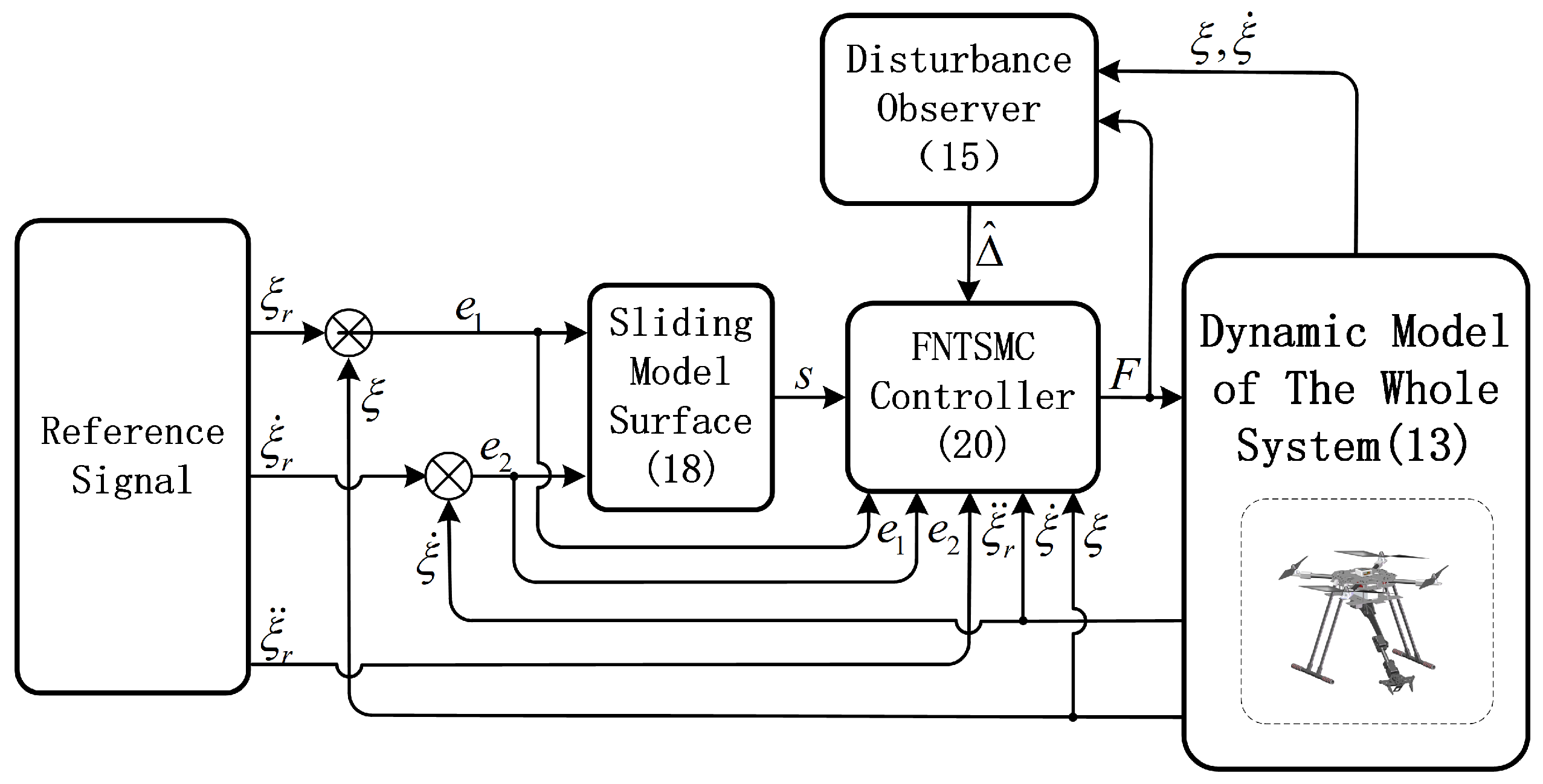
3. Control Design and Analysis

This section proposes a fast non-singular terminal sliding mode controller that drives both the quadrotor and the robotic arm to the desired operational position within a finite time. To suppress the destabilizing effects induced by the arm’s motion, a model-based disturbance observer is designed to estimate the lumped disturbances acting on the system.

For simplicity of expression, the function is defined as

$$\begin{array}{c}\hfill {\lfloor z\rceil }^{\gamma }=\mathrm{sign}\left(z\right){\left|z\right|}^{\gamma },\mathrm{for}\forall z\in \mathbb{R}\end{array}$$

(14)

where $\gamma \in {\mathbb{R}}^{+}$ is a positive constant, $\mathrm{sign}(·)$ denotes the signum function, and $|·|$ stands for the absolute value function.

Assumption 1.

The lumped disturbance $\Delta \left(t\right)$ is differentiable, and its first derivative is Lipschitz-continuous with a constant L.

Assumption 2.

The reference signal ${\xi }_r$ is twice continuously differentiable.

3.1. Design of a Model-Based Lumped Disturbance Observer

Based on the system model in (13), a finite-time lumped disturbance observer can be designed as

$$\begin{array}{cc}\hfill {\dot{z}}_0^i& =v_0^i+{\Lambda }_i(\xi ,F_i),{\dot{z}}_1^i=v_1^i,{\dot{z}}_2^i=v_2^i,\hfill \\ \hfill v_0^i& =-2L_i^{{\displaystyle \frac{1}{3}}}{\lfloor z_0^i-{\dot{\xi }}_i\rceil }^{{\displaystyle \frac{2}{3}}}+z_1^i,\hfill \\ \hfill v_1^i& =-1.5L_i^{{\displaystyle \frac{1}{2}}}{\lfloor z_1^i-v_0^i\rceil }^{{\displaystyle \frac{1}{2}}}+z_2^i,\hfill \\ \hfill v_2^i& =-1.1L_i{\lfloor z_2^i-v_1^i\rceil }^0,\hfill \\ \hfill {\widehat{\dot{\xi }}}_i& =z_0^i,{\widehat{\Delta }}_i\left(t\right)=D{z}_1^i,{\widehat{\dot{\Delta }}}_i\left(t\right)=D{z}_2^i,\hfill \end{array}$$

(15)

where $i=1,2,3,4$; the mapping $\Lambda (\xi ,F)$ is defined as $\Lambda (\xi ,F)=-D^{-1}(C\dot{\xi }+G-F)=$ ${[{\Lambda }_1(\xi ,F_i),{\Lambda }_2(\xi ,F_i),{\Lambda }_3(\xi ,F_i),{\Lambda }_4(\xi ,F_i)]}^{\mathrm{T}}$. The symbols ${\widehat{\dot{\xi }}}_i,{\widehat{\Delta }}_i\left(t\right),$${\widehat{\dot{\Delta }}}_i\left(t\right)$ denote the estimates of ${\dot{\xi }}_i,{\Delta }_i\left(t\right),{\dot{\Delta }}_i\left(t\right)$, respectively.

Combining (13) and (15), the estimation error is obtained as

$$\begin{array}{cc}\hfill {\epsilon }_0^i& =-2L^{{\displaystyle \frac{1}{3}}}{\lfloor {\epsilon }_0^i\rceil }^{{\displaystyle \frac{2}{3}}}+{\epsilon }_1^i,\hfill \\ \hfill {\epsilon }_1^i& =-1.5L^{{\displaystyle \frac{1}{2}}}{\lfloor {\epsilon }_1^i-{\dot{\epsilon }}_0^i\rceil }^{{\displaystyle \frac{1}{2}}}+{\epsilon }_2^i,\hfill \\ \hfill {\epsilon }_2^i& \in -1.1L^{{\displaystyle \frac{1}{4}}}{\lfloor {\epsilon }_2^i-{\dot{\epsilon }}_1^i\rceil }^0+[-L,L],\hfill \end{array}$$

(16)

where $i=1,2,3,4$ and the error variables are defined by ${\epsilon }_0^i=z_0^i-{\dot{\xi }}_i$, ${\epsilon }_1^i=z_1^i-D^{-1}{\Delta }_i\left(t\right)$, ${\epsilon }_2^i=z_2^i-D^{-1}{\dot{\Delta }}_i\left(t\right)$. Based on [31], the estimation error system in (16) is finite-time-stable and bounded. Specifically, there exist positive constants $C_1$ and $C_2$, such that $|{\epsilon }_1^i|\le C_1$, $|{\epsilon }_2^i|\le C_2$, and a finite time $T>0$ for which ${\epsilon }_1^i\left(T\right)={\epsilon }_2^i\left(T\right)=0$. By defining the vector errors ${\epsilon }_j={[{\epsilon }_j^1,{\epsilon }_j^2,{\epsilon }_j^3,{\epsilon }_j^4]}^{\mathrm{T}}$ with $j=1,2$, it follows that $\left|\right|{\epsilon }_1{\left|\right|}_2\le 2C_1$, $\left|\right|{\epsilon }_2{\left|\right|}_2\le 2C_2$, and both ${\epsilon }_1$ and ${\epsilon }_2$ converge to zero within the finite time.

3.2. Design of a Composite Finite-Time Tracking Controller

The tracking errors are defined as $e_1=\xi -{\xi }_r$ and $e_2=\dot{\xi }-{\dot{\xi }}_r$. Hence, their time derivatives can be expressed as

$$\begin{array}{cc}\hfill {\dot{e}}_1& =e_2,\hfill \\ \hfill {\dot{e}}_2& =-D^{-1}C\dot{\xi }-D^{-1}G+D^{-1}F+D^{-1}\Delta \left(t\right)-{\ddot{\xi }}_r.\hfill \end{array}$$

(17)

The nonlinear fast terminal sliding mode surface is defined as follows:

$$\begin{array}{c}\hfill s=e_1+{\lambda }_1{\lfloor e_1\rceil }^{{\gamma }_1}+{\lambda }_2{\lfloor e_2\rceil }^{{\gamma }_2},\end{array}$$

(18)

where ${\lambda }_1>0,{\lambda }_2>0,1<{\gamma }_2<2$ and ${\gamma }_1>{\gamma }_2$. The time derivative of the sliding surface s can be expressed as

$$\begin{array}{cc}\hfill \dot{s}& ={\dot{e}}_1+{\lambda }_1{\gamma }_1|e_1{|}^{{\gamma }_1-1}{\dot{e}}_1+{\lambda }_2{\gamma }_2{\left|e_2\right|}^{{\gamma }_2-1}{\dot{e}}_2,\hfill \\ \hfill & ={\dot{e}}_1+{\lambda }_1{\gamma }_1|e_1{|}^{{\gamma }_1-1}{e}_2+{\lambda }_2{\gamma }_2{\left|e_2\right|}^{{\gamma }_2-1}(\begin{array}{c}\hfill -D^{-1}C\dot{\xi }-D^{-1}G\end{array}+D^{-1}F+D^{-1}\Delta \left(t\right)-{\ddot{\xi }}_r).\hfill \end{array}$$

(19)

The control input F is defined as follows:

$$\begin{array}{cc}\hfill F& =F_a+F_b,\hfill \\ \hfill F_a& =C\dot{\xi }+G+D{\ddot{\xi }}_r-\widehat{\Delta }\left(t\right)-D({\displaystyle \frac{1}{{\lambda }_2{\gamma }_2}}{\lfloor e_2\rceil }^{2-{\gamma }_2}+{\displaystyle \frac{{\lambda }_1{\gamma }_1}{{\lambda }_2{\gamma }_2}}{\lfloor e_2\rceil }^{2-{\gamma }_2}|e_1{|}^{{\gamma }_1-1}),\hfill \\ \hfill F_b& =-D(k_{1}s+k_2{\lfloor s\rceil }^{{\gamma }_3}),\hfill \end{array}$$

(20)

where $k_1>0$ and $k_2>0$ are positive constants and $0<{\gamma }_3<1$. Substituting (20) into (19), we get

$$\begin{array}{c}\hfill \dot{s}=-{\lambda }_2{\gamma }_2{\left|e_2\right|}^{{\gamma }_2-1}(k_{1}s+k_2{\lfloor s\rceil }^{{\gamma }_3}-e_d),\end{array}$$

(21)

where $e_d=D^{-1}\Delta \left(t\right)-D^{-1}\widehat{\Delta }\left(t\right)$.

3.3. Closed-Loop System Stability Analysis

Without loss of generality, we concentrate on the first state of the system and employ the Lyapunov method for stability analysis. A finite-time-bounded Lyapunov function is defined as follows:

$$\begin{array}{c}\hfill V\left(s\right)={\displaystyle \frac{1}{2}}{s}^2+{\displaystyle \frac{1}{2}}{e_d}^2.\end{array}$$

(22)

The time derivative of the Lyapunov function defined above can be written as

$$\begin{array}{cc}\hfill \dot{V}\left(s\right)& =s\dot{s}+e_d{\dot{e}}_d,\hfill \\ \hfill & =-{\lambda }_2{\gamma }_2|e_2{|}^{{\gamma }_2-1}(k_1{s}^2+k_2{\left|s\right|}^{{\gamma }_3+1}-e_{d}s)+e_d{\dot{e}}_d.\hfill \end{array}$$

(23)

According to the results established in Section 3.1, we have $|e_d| = |{\epsilon }_1^1| \le C_1$ and $|{\dot{e}}_d| = |{\epsilon }_2^1| \le C_2$. Consequently,

$$\begin{array}{cc}\hfill \dot{V}\left(s\right)& \le {\lambda }_2{\gamma }_2|e_2{|}^{{\gamma }_2-1}(-k_1{s}^2-k_2{\left|s\right|}^{{\gamma }_3+1}+C_1\left|s\right|)+C_1{C}_2\hfill \\ \hfill & ={\lambda }_2{\gamma }_2|e_2{|}^{{\gamma }_2-1}[-k_1\left(\right|s|-C_1\left)\right|s|-k_2{\left|s\right|}^{{\gamma }_3+1}]+C_1{C}_2.\hfill \end{array}$$

(24)

When $\left|s\right|\ge C_1$, the Lyapunov derivative satisfies $\dot{V}\left(s\right)\le C_1{C}_2$, implying that the system states remain bounded. Hence, there exists a finite time $T^{\prime }$ such that for every $t\ge T^{\prime }$ we have $e_d\to 0$, ${\dot{e}}_d\to 0$, and $V\left(s\right)\to s^2/2$. Therefore,

$$\begin{array}{cc}\hfill \dot{V}\left(s\right)& =s\dot{s}\hfill \\ \hfill & \le -{\lambda }_2{\gamma }_2|e_2{|}^{{\gamma }_2-1}(k_1{s}^2+k_2{\left|s\right|}^{{\gamma }_3+1})\hfill \\ \hfill & =-{\lambda }_2{\gamma }_2{\left|e_2\right|}^{{\gamma }_2-1}(2k_{1}V+2^{{\displaystyle \frac{{\gamma }_3+1}{2}}}{k}_2{V}^{{\displaystyle \frac{{\gamma }_3+1}{2}}})\hfill \\ \hfill & =-n_{1}V-n_2{V}^{{\displaystyle \frac{{\gamma }_3+1}{2}}},\hfill \end{array}$$

(25)

where $n_1=2{\lambda }_2{\gamma }_2{\left|e_2\right|}^{{\gamma }_2-1}{k}_1$ and $n_2=2^{({\gamma }_3+1)/2}{\lambda }_2{\gamma }_2{\left|e_2\right|}^{{\gamma }_2-1}{k}_2$. Hence, the closed-loop system is finite-time-stable.

When $s=0$, it can be obtained that

$$\begin{array}{c}\hfill e_2=-{\lambda }_2^{-{\displaystyle \frac{1}{{\gamma }_2}}}\mathrm{sign}\left(e_1\right)(|e_1|+{\lambda }_1|e_1{{|}^{{\gamma }_1})}^{{\displaystyle \frac{1}{{\gamma }_2}}}.\end{array}$$

(26)

Define the Lyapunov function $W=e_1^2/2$, whose time derivative is

$$\begin{array}{cc}\hfill \dot{W}& =-{\lambda }_2^{-{\displaystyle \frac{1}{{\gamma }_2}}}|e_1|((|e_1|+{\lambda }_1|e_1{|}^{{\gamma }_1}{)}^{{\displaystyle \frac{1}{{\gamma }_2}}})\hfill \\ \hfill & \le -{\lambda }_2^{-{\displaystyle \frac{1}{{\gamma }_2}}}|e_1|(|e_1{|}^{{\displaystyle \frac{1}{{\gamma }_2}}}+{\lambda }_1^{{\displaystyle \frac{1}{{\gamma }_2}}}|e_1{|}^{{\displaystyle \frac{{\gamma }_1}{{\gamma }_2}}})2^{{\displaystyle \frac{1}{{\gamma }_2}}-1}\hfill \\ \hfill & =-{\lambda }_2^{-{\displaystyle \frac{1}{{\gamma }_2}}}|e_1{|}^{1+{\displaystyle \frac{1}{{\gamma }_2}}}{2}^{{\displaystyle \frac{1}{{\gamma }_2}}-1}-{\lambda }_1^{{\displaystyle \frac{1}{{\gamma }_2}}}{\lambda }_2^{-{\displaystyle \frac{1}{{\gamma }_2}}}{|e_1|}^{1+{\displaystyle \frac{{\gamma }_1}{{\gamma }_2}}}{2}^{{\displaystyle \frac{1}{{\gamma }_2}}-1}\hfill \\ \hfill & =-{({\displaystyle \frac{2}{{\lambda }_2}})}^{{\displaystyle \frac{1}{{\gamma }_2}}}{W}^{{\displaystyle \frac{1+{\gamma }_2}{2{\gamma }_2}}}-{({\displaystyle \frac{{\lambda }_1}{{\lambda }_2}})}^{{\displaystyle \frac{1}{{\gamma }_2}}}{2}^{{\displaystyle \frac{1+{\gamma }_2}{2{\gamma }_2}}}{W}^{{\displaystyle \frac{{\gamma }_1+{\gamma }_2}{2{\gamma }_2}}}\hfill \\ \hfill & =-c_3{W}^{{\displaystyle \frac{1+{\gamma }_2}{2{\gamma }_2}}}-c_4{W}^{{\displaystyle \frac{{\gamma }_1+{\gamma }_2}{2{\gamma }_2}}},\hfill \end{array}$$

(27)

where $c_3={(2/{\lambda }_2)}^{1/{\gamma }_2}$ and $c_4={({\lambda }_1/{\lambda }_2)}^{1/{\gamma }_2}{2}^{(1+{\gamma }_2)/\left(2{\gamma }_2\right)}$. Consequently, the Lyapunov function W is negative definite. When $e_1$ converges to zero in finite time, $e_2$ also vanishes within finite time and the closed-loop system attains finite-time stability.

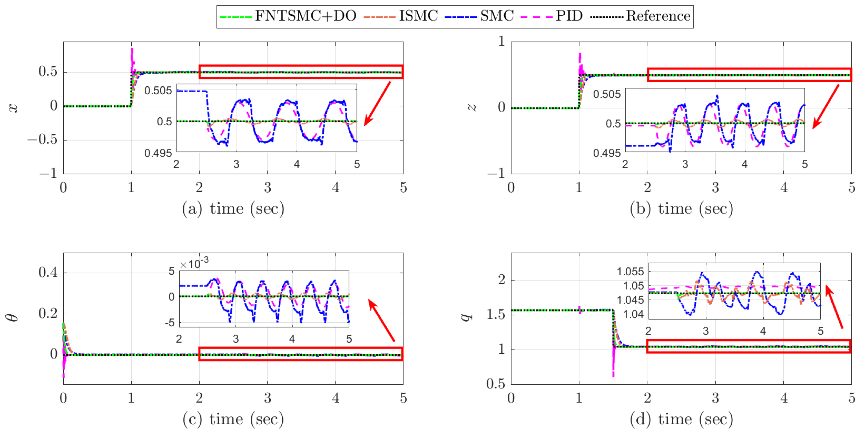
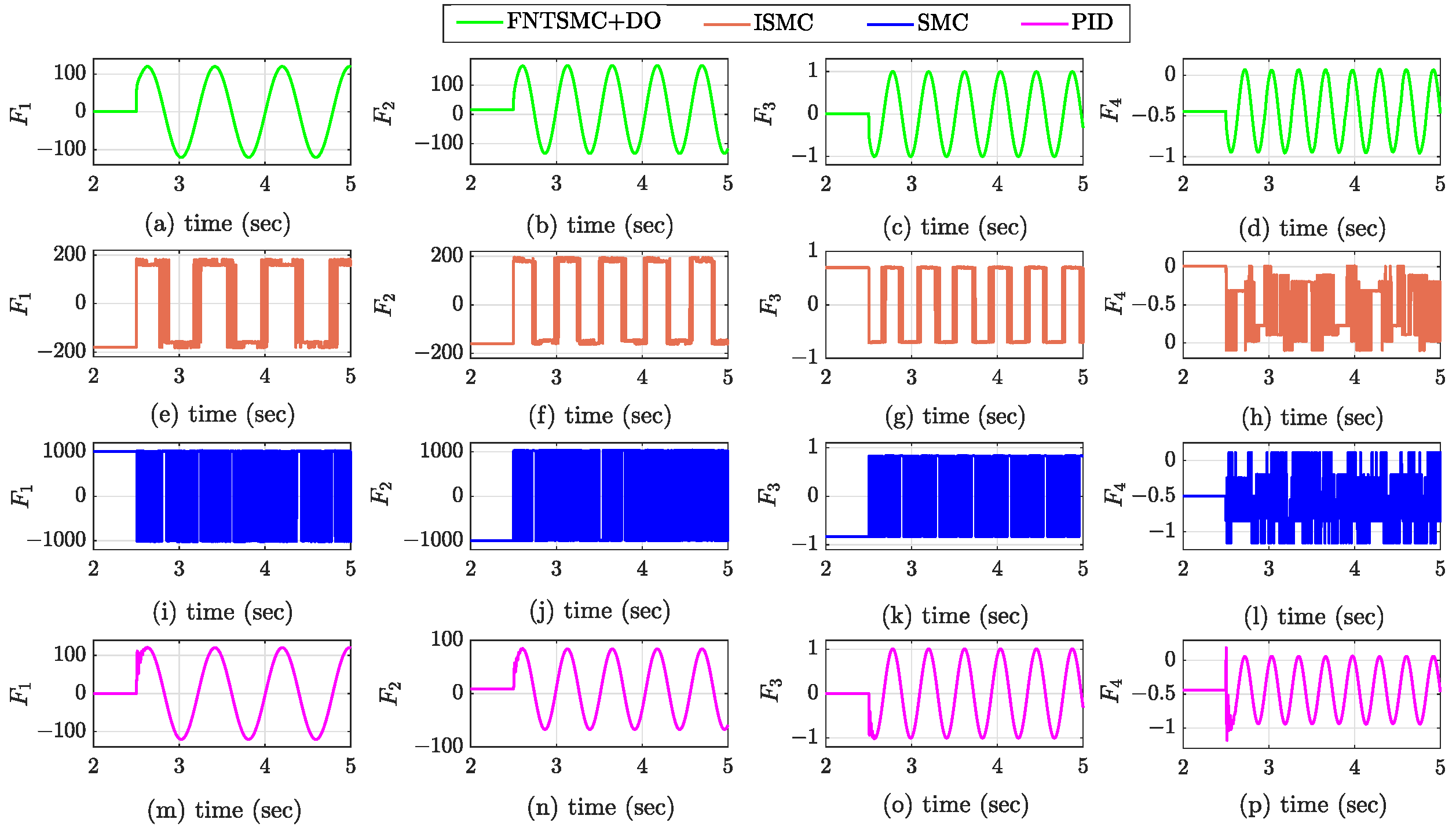
4. Simulation Results and Analysis

To verify the effectiveness of the proposed dynamic model and control scheme, trajectory-tracking and dynamic-grasping simulations were performed in a MATLAB Simulink 2020b environment using a laptop with an Intel i9-13900HX CPU and NVIDIA RTX 4060 GPU specifications. The system parameters are listed in

Table 1. Parameters of the quadrotor with a robotic arm system.

Parameter	Value
Mass of the quadrotor body: ${\overline{m}}_b-\Delta m_b/\left(\mathrm{kg}\right)$	$1.50\pm 0.01$
Mass of the robotic arm link: ${\overline{m}}_1-\Delta m_1/\left(\mathrm{kg}\right)$	$0.18\pm 0.01$
Length of the robotic arm link: ${\overline{l}}_1-\Delta l_1/\left(\mathrm{m}\right)$	$0.13\pm 0.01$
Inertia tensor of the quadrotor along	$(1.38\pm 0.01)\times {10}^{-2}$
the y axis: ${\overline{I}}_y-\Delta I_y/$(kg·m−2)
Inertia tensor of the robotic arm along	$(0.31\pm 0.01)\times {10}^{-2}$
the y axis: ${\overline{I}}_1-\Delta I_1/$(kg·m−2)

.

Each parameter comprises a true value with an uncertainty term, thereby emulating the influence of measurement errors on the real system. The controller gains were selected through repeated trials and are determined as ${\lambda }_1=300,{\lambda }_2=3.5,{\gamma }_1=1.2,{\gamma }_2=1.1,{\gamma }_3=0.64,k_1=80,k_2=80.$ The simulation block diagram of the quadrotor with a robotic arm system control architecture is depicted in Figure 2.

To evaluate the effectiveness of the proposed FNTSMC strategy, the system is initialized at $T_0={[0,0,0]}^{\mathrm{T}}\mathrm{m}$ with a pitch angle $\theta =\pi /20\mathrm{rad}$ and a joint angle $q=\pi /2\mathrm{rad}$. At $t=1\mathrm{s}$, a step command drives the system toward the target position $T_1={[0.5,0.5,0]}^{\mathrm{T}}\mathrm{m}$. At $t=1.5\mathrm{s}$, the joint rotates from $\pi /2\mathrm{rad}$ to $\pi /3\mathrm{rad}$ to grasp an object, and for $t>2.5\mathrm{s}$, the system is subjected to disturbances ${\Delta }_1\left(t\right)=-120\sin \left(8(t-2.5)+\pi /6\right)$, ${\Delta }_2\left(t\right)=-150\sin \left(12(t-2.5)+\pi /10\right)$, ${\Delta }_3\left(t\right)=\sin \left(15(t-2.5)+\pi /10\right)$, and ${\Delta }_4\left(t\right)=0.5\sin \left(20(t-2.5)+\pi /10\right)$. The performance of the FNTSMC controller is compared with integral sliding mode controller (ISMC), sliding mode controller (SMC), and PID controller. The corresponding simulation results are summarized in Figure 3 and

Table 2. A comparison of the algorithmic performance between FNTSMC, ISMC, SMC, and PID.

Channel	Algorithm	Adjust Time	Overshoot	IAE	ITAE
x	FNTSMC	0.060 s	0.00%	0.0083 m·s	0.0085 m·s2
	ISMC	0.109 s	1.75%	0.0224 m·s	0.0232 m·s2
	SMC	0.156 s	0.00%	0.0331 m·s	0.0396 m·s2
	PID	0.088 s	68.16%	0.0107 m·s	0.0111 m·s2
z	FNTSMC	0.059 s	0.00%	0.0083 m·s	0.0085 m·s2
	ISMC	0.109 s	0.87%	0.0224 m·s	0.0233 m·s2
	SMC	0.164 s	0.00%	0.0331 m·s	0.0390 m·s2
	PID	0.087 s	71.80%	0.0118 m·s	0.0126 m·s2
$\theta$	FNTSMC	0.063 s	0.00%	0.0033 rad·s	$7.3760\times {10}^{-5}$ rad·s2
	ISMC	0.140 s	0.62%	0.0103 rad·s	$4.9647\times {10}^{-4}$ rad·s2
	SMC	0.168 s	0.00%	0.0132 rad·s	0.0067 rad·s2
	PID	0.062 s	71.38%	0.0021 rad·s	$7.9439\times {10}^{-5}$ rad·s2
q	FNTSMC	0.043 s	0.00%	0.0060 rad·s	0.0091 rad·s2
	ISMC	0.108 s	0.87%	0.0236 rad·s	0.0361 rad·s2
	SMC	0.154 s	0.00%	0.0308 rad·s	0.0474 rad·s2
	PID	0.029 s	83.42%	0.0062 rad·s	0.0095 rad·s2

.

Regarding adjust time, the FNTSMC scheme outperforms both ISMC and SMC. The FNTSMC settles in less than 0.10 s on every channel, whereas the ISMC and SMC responses each require more than 0.10 s. Specifically, in the $\theta$ and q channels, the FNTSMC achieves settling times of 0.063 s and 0.043 s, respectively, more than a two-fold reduction relative to ISMC and SMC. As for overshoot, FNTSMC exhibits none across all channels, thereby eliminating the adverse effects commonly associated with overshoot. ISMC keeps overshoot below 2%, which has only a minor impact, while SMC is overshoot-free yet displays the longest settling time among the four controllers. By contrast, PID control incurs an overshoot greater than 60% on every channel and induces severe oscillations. In a physical platform, such rapid control-signal reversals could easily lead to loss of stability. And it shows that the proposed algorithm reduces the regulation time by more than 45% compared to ISMC and SMC and decreases the overshoot by at least 68% compared to the PID controller. At the same time, it can be observed that the (Integral of Absolute Error) IAE and (Integral of Time-weighted Absolute Error) ITAE of the control algorithm proposed are all smaller than those of other algorithms in each channel. In addition, the proposed finite-time lumped-disturbance observer effectively compensates for external perturbations. Throughout the 2–5 s interval, no appreciable disturbance is observed in any channel, confirming that the observer identifies and attenuates disturbances within finite time, as illustrated in Figure 4.

The system control inputs for different algorithms are shown in Figure 5. It can be observed that the proposed method encountered no chattering phenomena compared to the ISMC and SMC algorithms. This advantage can make the system control smoother.

5. Conclusions

This paper proposes a novel modeling and control framework for an aerial work quadrotor with a robotic arm. An energy-conservation-based integrated modeling technique treats the quadrotor and robtic arm as a single unified system, yielding a concise second-order dynamic model. Coupling this model with a fast non-singular terminal sliding mode controller enables the finite-time tracking of the desired trajectory and joint angle. To further enhance stability during arm motion, a model-based finite-time disturbance observer is incorporated into the controller design, and Lyapunov finite time theory is employed to rigorously prove closed-loop stability. Simulation results demonstrate that, compared with ISMC, SMC, and PID controllers, the proposed approach delivers markedly superior performance, providing an effective solution for engineering applications of aerial robotic systems. In the future, we plan to extend the system model to a full-degree-of-freedom plane and initiate physical experiments to validate the proposed algorithm.

References

1. Ning, B.; Han, Q.; Zuo, Z.; Jin, J.; Zheng, J. Collective behaviors of mobile robots beyond the nearest neighbor rules with switching topology. IEEE Trans. Cybern. 2017, 48, 1577–1590. [Google Scholar] [CrossRef] [PubMed]
2. Yu, B.; Du, H.; Wen, G.; Zhou, J.; Zheng, D. A vector-type finite-time output-constrained control algorithm and its application to a mobile robot. Robot. Intell. Autom. 2025, 45, 306–313. [Google Scholar] [CrossRef]
3. Zhao, J.; Zhang, J.; Li, D.; Wang, D. Vision-Based Anti-UAV Detection and Tracking. IEEE Trans. Intell. Transp. Syst. 2022, 23, 25323–25334. [Google Scholar] [CrossRef]
4. Cui, J.; Qin, Y.; Wu, Y.; Shao, C.; Yang, H. Skip Connection YOLO Architecture for Noise Barrier Defect Detection Using UAV-Based Images in High-Speed Railway. IEEE Trans. Intell. Transp. Syst. 2023, 24, 12180–12195. [Google Scholar] [CrossRef]
5. Han, L.; Zhou, Z.; Li, M.; Geng, H.; Li, G.; Zhang, M. Energy-Coupling-Based Control for Unmanned Quadrotor Transportation Systems: Exploiting Beneficial State-Coupling Effects. Actuators 2025, 14, 91. [Google Scholar] [CrossRef]
6. Zhu, X.; Gao, Y.; Li, Y.; Li, B. Fast Dynamic P-RRT*-Based UAV Path Planning and Trajectory Tracking Control Under Dense Obstacles. Actuators 2025, 14, 211. [Google Scholar] [CrossRef]
7. Wang, G.; Chen, Y.; An, P.; Hong, H.; Hu, J. UAV-YOLOv8: A Small-Object-Detection Model Based on Improved YOLOv8 for UAV Aerial Photography Scenarios. Sensors 2023, 23, 7190. [Google Scholar] [CrossRef] [PubMed]
8. Jiao, R.; Liu, Y.; He, H.; Ma, X.; Li, Z. A Deep Learning Model for Small-size Defective Components Detection in Power Transmission Tower. IEEE Trans. Power Deliv. 2022, 37, 2551–2561. [Google Scholar] [CrossRef]
9. Jeong, J.; Park, S.; Lee, S.; Youn, D.; Kim, M.J. Designing an End-to-End UAV System for Insulator Inspection Under Transmission Tower Environments. In Proceedings of the International Conference on Electronics, Information, and Communication (ICEIC), Taipei, Taiwan, 28–31 January 2024; pp. 1–4. [Google Scholar]
10. Zhuo, H.; Yang, Z.; You, Y.; Xu, N.; Liao, L.; Wu, J.; He, J. A Hierarchical Control Method for Trajectory Tracking of Aerial Manipulators Arms. Actuators 2024, 13, 333. [Google Scholar] [CrossRef]
11. Ghadiok, V.; Goldin, J.; Ren, W. On the design and development of attitude stabilization, vision-based navigation, and aerial gripping for a low-cost quadrotor. Auton. Robot. 2012, 33, 41–68. [Google Scholar] [CrossRef]
12. Fiaz, U.A.; Abdelkader, M.; Shamma, J.S. An intelligent gripper design for autonomous aerial transport with passive magnetic grasping and dual-impulsive release. In Proceedings of the IEEE/ASME International Conference on Advanced Intelligent Mechatronics (AIM), Auckland, New Zealand, 9–12 July 2018; pp. 1027–1032. [Google Scholar]
13. Chermprayong, P.; Zhang, K.; Xiao, F.; Kovac, M. An integrated delta manipulator for aerial repair: A new aerial robotic system. IEEE Robot. Autom. Mag. 2019, 26, 54–66. [Google Scholar] [CrossRef]
14. Qian, L.; Liu, H.H. Path-following control of a quadrotor UAV with a cable-suspended payload under wind disturbances. IEEE Trans. Ind. Electron. 2019, 67, 2021–2029. [Google Scholar] [CrossRef]
15. Jafarinasab, M.; Sirouspour, S.; Dyer, E. Model-Based Motion Control of a Robotic Manipulator with a Flying Multirotor Base. IEEE/ASME Trans. Mechatronics 2019, 24, 2328–2340. [Google Scholar] [CrossRef]
16. Wang, M.; Lyu, S.; Liu, Q.; Yang, Z.; Guo, K.; Yu, X. Precise End-Effector Control for an Aerial Manipulator Under Composite Disturbances: Theory and Experiments. IEEE Trans. Autom. Sci. Eng. 2024, 22, 4006–4021. [Google Scholar] [CrossRef]
17. Li, Z.; Yang, Y.; Yu, X.; Liu, C.; Kaynak, O.; Gao, H. Fixed-Time Control of a Novel Thrust-Vectoring Aerial Manipulator via High-Order Fully Actuated System Approach. IEEE/Asme Trans. Mechatronics 2024, 30, 1084–1095. [Google Scholar] [CrossRef]
18. Liang, J.; Chen, Y.; Wu, Y.; Miao, Z.; Zhang, H.; Wang, Y. Adaptive Prescribed Performance Control of Unmanned Aerial Manipulator With Disturbances. IEEE Trans. Autom. Sci. Eng. 2023, 20, 1804–1814. [Google Scholar] [CrossRef]
19. Zhu, W.; Du, H. Global Uniform Finite-Time Output Feedback Stabilization for Disturbed Nonlinear Uncertain Systems: Backstepping-like Observer and Nonseparation Principle Design. SIAM J. Control Optim. 2024, 62, 1717–1736. [Google Scholar] [CrossRef]
20. Kim, S.; Choi, S.; Kim, H.J. Aerial Manipulation Using a Quadrotor with a Two DOF Robotic Arm. In Proceedings of the IEEE/RSJ International Conference on Intelligent Robots and Systems (IROS), Tokyo, Japan, 3–7 November 2013; pp. 4990–4995. [Google Scholar]
21. Luna, A.L.; Vega, I.C.; Carranza, J.M. Gain-Scheduling and PID Control for an Autonomous Aerial Vehicle with a Robotic Arm. In Proceedings of the IEEE 2nd Colombian Conference on Robotics and Automation (CCRA), Barranquilla, Colombia, 1–3 November 2018; pp. 1–6. [Google Scholar]
22. Kim, M.J.; Kondak, K.; Ott, C. A Stabilizing Controller for Regulation of UAV With Manipulator. IEEE Robot. Autom. Lett. 2018, 3, 1719–1726. [Google Scholar] [CrossRef]
23. Kim, S.; Seo, H.; Choi, S.; Kim, H.J. Vision-Guided Aerial Manipulation Using a Multirotor With a Robotic Arm. IEEE/ASME Trans. Mechatronics 2016, 21, 1912–1923. [Google Scholar] [CrossRef]
24. Ouyang, Z.; Mei, R.; Liu, Z.; Wei, M.; Zhou, Z.; Cheng, H. Control of an Aerial Manipulator Using a Quadrotor with a Replaceable Robotic Arm. In Proceedings of the IEEE International Conference on Robotics and Automation (ICRA), Xi’an, China, 30 May–5 June 2021; pp. 153–159. [Google Scholar]
25. Afifa, R.; Ali, S.; Pervaiz, M.; Iqbal, J. Adaptive Backstepping Integral Sliding Mode Control of a MIMO Separately Excited DC Motor. Robotics 2023, 12, 105. [Google Scholar] [CrossRef]
26. Ali, K.; Ulah, S.; Mehmood, A.; Mostafa, H.; Marey, M.; Iqbal, J. Adaptive FIT-SMC Approach for an Anthropomorphic Manipulator With Robust Exact Differentiator and Neural Network-Based Friction Compensation. IEEE Access 2022, 10, 3378–3389. [Google Scholar] [CrossRef]
27. Lippiello, V.; Ruggiero, F. Exploiting Redundancy in Cartesian Impedance Control of UAVs Equipped with a Robotic Arm. In Proceedings of the IEEE/RSJ International Conference on Intelligent Robots and Systems (IROS), Vilamoura-Algarve, Portugal, 7–12 October 2012; pp. 3768–3773. [Google Scholar]
28. Nail, M.; Jänne, N.; Ma, O.; Arellano, G.; Atkins, E.; Gillespie, R.B. Simplifying Aerial Manipulation Using Intentional Collisions. In Proceedings of the IEEE International Conference on Robotics and Automation (ICRA), London, UK, 29 May–2 June 2023; pp. 5359–5365. [Google Scholar]
29. Wang, T.; Umemoto, K.; Endo, T.; Matsuno, F. Modeling and Control of a Quadrotor UAV Equipped With a Flexible Arm in Vertical Plane. IEEE Access 2021, 9, 98476–98489. [Google Scholar] [CrossRef]
30. Abhishek, V.; Srivastava, V.; Mukherjee, R. Towards a heterogeneous cable-connected team of UAVs for aerial manipulation. In Proceedings of the American Control Conference (ACC), New Orleans, LA, USA, 25–28 May 2021; pp. 54–59. [Google Scholar]
31. Davila, J.; Fridman, L.; Levant, A. Second-Order Sliding-Mode Observer for Mechanical Systems. IEEE Trans. Autom. Control 2005, 50, 1785–1789. [Google Scholar] [CrossRef]
Figure 1. Diagram of the quadrotor with a robotic arm.
Actuators 14 00357 g001
Figure 2. Simulation block diagram of the quadrotor with a robotic arm system control architecture, and (·) representing the equation number in this paper.
Actuators 14 00357 g002
Figure 3. Response curves of the quadrotor with a robotic arm system in x , z , θ , q channels, (a) x channel response curve, (b) z channel response curve, (c) θ channel response curve, (d) q channel response curve.
Actuators 14 00357 g003
Figure 4. Interference with the observation results of the quadrotor with a robotic arm system in x , z , θ , q channels, (a) x channel interference observation result, (b) x channel interference observation result, (c) x channel interference observation result, (d) x channel interference observation result.
Actuators 14 00357 g004
Figure 5. The control input of the quadrotor with a robotic arm system for different algorithms, (ad) control input of F 1 F 4 channel with FNTSMC algorithm with disturbance observer, (ch) control input of F 1 F 4 channel with ISMC algorithm, (il) control input of F 1 F 4 channel with SMC algorithm, (mp) control input of F 1 F 4 channel with PID algorithm.
Actuators 14 00357 g005