Gyro-System for Guidance with Magnetically Suspended Gyroscope, Using Control Laws Based on Dynamic Inversion

Abstract

The authors have designed a gyro-system for orientation (guidance) and stabilization, with two gimbals and a rotor in magnetic suspension (AMB—Active Magnetic Bearing) usable for self-guided rockets. The gyro-system (DGMSGG—double gimbal magnetic suspension gyro-system for guidance) orients and stabilizes the target coordinator’s axis (CT) and, at the same time, the AMB–rotor’s axis so that they overlap the guidance line (the target line). DGMSGG consists of two decoupled systems: one for canceling the AMB–rotor translations along the precession axes (induced by external disturbing forces), the other for canceling the AMB–rotor rotations relative to the CT-axis (induced by external disturbing moments) and, at the same time, for controlling the gimbals’ rotations, so that the AMB–rotor’s axis overlaps the guidance line. The nonlinear DGMSGG model is decomposed into two sub-models: one for the AMB–rotor’s translation, the other for the AMB–rotor’s and gimbals’ rotation. The second sub-model is described first by nonlinear state equations. This model is reduced to a second order nonlinear matrix—vector form with respect to the output vector. The output vector consists of the rotation angles of the AMB–rotor and the rotation angles of the gimbals. For this purpose, a differential geometry method, based on the use of the output vector’s gradient with respect to the nonlinear state functions, i.e., based on Lie derivatives, is used. This equation highlights the relative degree (equal to 2) with respect to the variables of the output vector and allows for the use of the dynamic inversion method in the design of stabilization and guidance controllers (of P.I.D.- and PD-types), as well as in the design of the related linear state observers. The controller of the subsystem intended for AMB–rotor’s translations control is chosen as P.I.D.-type, which leads to the cancellation of both its translations and its translation speeds. The theoretical results are validated through numerical simulations, using Simulink/Matlab models.

1. Introduction

A large class of gyro-systems, based on fast astatic gyros (GAR), displaced in classical mechanical suspension or in magnetic suspension—Active Magnetic Bearing, contains actuators used for attitude stabilization and orientation of mini-satellites [1,2,3,4,5,6,7], as well as for stabilization and orientation of inertial platforms, or for orientation on a direction imposed in the process of aerospace navigation and guidance. Gyroscopic actuators are known as Control Moment Gyros. These ones can contain classic GARs or magnetically suspended gyros, with a single gimbal (SGMSCMG) or with two gimbals (DGMSCMG); they may be equipped with gyroscopic rotors with constant or variable spin rate (SGVSCMG or DGVSCMG). The advantages of using MSCMGs are the following: elimination of the need for lubrication, low noise, low vibrations, and longevity [8,9,10,11,12,13]. SGCMGs are used in various cluster configurations [14]. The construction and structure of SGMSCMGs and of DGMSCMGs, as well as of DGMSGG, allow for the decoupling of the AMB–rotor translation dynamics from its rotation dynamics and from the gimbals’ rotation dynamics, and implicitly allow the decoupling of the translation control system from the rotor’s and gyroscopic gimbals’ rotation control systems [15,16,17,18,19,20,21,22,23,24,25,26,27,28,29].

Some of the papers mentioned in the reference list refer to the architecture and the constructive and technological particularities of gyroscopic equipment with one or two gimbals and a rotor in magnetic suspension. Whether this gyro equipment is used as actuators or as orientation and stabilization (positioning) systems, in the specialized scientific literature, they are all called CMGs (SGMSCMG or DGMSCMG).

Leaving aside the considerations regarding the constructive and technological particularities common to the above-mentioned two categories of equipment (actuators and positioning systems), there are essential differences between them. Thus, in the case of DGMSCMGs, on the one hand, the linear and angular displacements of the gimbals are controlled, and on the other hand, the angular rates applied to the gimbals are also controlled; the gyro-system reacts to the angular rates of the gimbals through gyroscopic torques. So, the gyroscopic phenomenon that underlies the functioning of DGMSCMGs is the gyroscopic torque, while gyro-systems for orientation and stabilization (in this case DGMSGGs) operate based on the gyroscopic phenomenon known as the gyroscopic effect (gyro-effect); the moments applied to the gimbals produce angular rates of gyro-rotor’s precession and, implicitly, gimbals’ angles of rotation. For these reasons, it is necessary to identify and name DGMSGGs differently from DGMSCMGs, so that we cannot compare the performances of the two types of equipment.

The DGMSGG architecture is a new engineering solution. The novelty in this paper consists of: (a) mounting a new device—the target coordinator (CT)—on the inner gimbal of the DGMS; (b) using control laws based on the dynamic inversion concept.

To control the dynamics of actuators and gyro-systems for stabilization and orientation/guidance, various linear control laws are used, such as P.D.-, P.I.-, P.I.D.-type, back-stepping, sliding mode [10,13,17,21,25,26], but also adaptive-type [14,15,21,23,24,25,27,28,30,31,32,33,34,35,36,37].

In this paper, a guidance gyro-system structure with two gyroscopic gimbals and a magnetically suspended rotor is designed, using the concept of dynamic inversion, with the possibility of use on self-guided rockets. Such a gyro-system has as its main role to control the direction of the AMB–rotor axis (the line of sight), orienting it in the direction of the target line (the guidance line). Starting from the nonlinear equations of the rotor dynamics and of the gyroscopic gimbals [29], the subsystems for automatic control of the AMB–rotor’s translation vector, as well as of its rotation AMB—rotor’s and of the gyroscopic gimbals’ vectors, are designed. Differential geometry theory is used to determine the relative degrees of the output variables [16,18,19]. The automatic control subsystems of DGMSGG’s dynamics use linear dynamic P.D.-type compensators, linear state observers, and reference models, as well as a P.I.D.-type guidance controller.

The method of dynamic inversion is adequate for the control of nonlinear dynamics, whose dimensional parameters (values of equations’ coefficients) are known, e.g., the kinetic moments, the moments of inertia, the physical parameters of the gyroscopic rotors, and of the drive engines from the DGMSGG architecture, etc. Also, the stabilization and orientation control systems do not require feedback and, therefore, sensors or transducers other than those for measuring the gyroscopic rotors’ total linear displacements and for measuring the gimbals’ rotation angles. For these reasons, control techniques based on dynamic inversion instead of back-stepping, sliding mode, or predictive control techniques are preferred. The dynamic inversion method, successfully used by the authors of this paper in previous papers (such as in [27]), also uses a neural network, which provides an adaptive component of the control law, in order to compensate for the dynamic inversion error; the neural network works as a dynamic inversion error estimator (observer). The results obtained by using the two dynamic inversion control architectures (with or without neural network) are comparable; moreover, compared to other control laws, extremely small stabilization and orientation errors are obtained, sometimes even equal to zero.

The paper is structured as follows. Section 2 presents the structure of the DGMSGG, its frames, and its related angular parameters. In Section 3, nonlinear dynamic models of the AMB–rotor and of the gyroscopic gimbals are presented. Section 4 is reserved for presenting the structure of the DGMSGG’s automatic control system, which is based on the dynamic inversion concept, while in Section 5, its subsystems are designed. In Section 6, the results of numerical simulations based on Matlab/Simulink models and the related discussions are presented. In the last section, the conclusions of the paper are formulated.

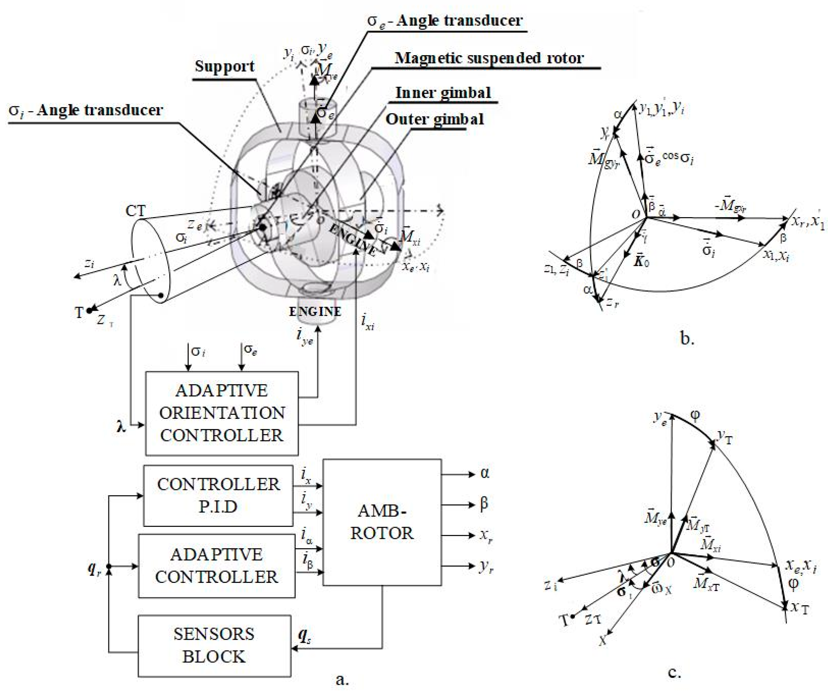
2. The Structure of a DGMSGG, the Reference Frames, and the Defining Angular Parameters

The structure of the used DGMSGG is the one described in [27], consisting of the following main parts: (a) gyro-equipment with two gimbals and a rotor in magnetic suspension (AMB–rotor) [16] to which a CT (target coordinator) is attached; (b) control motors; (c) transducers arranged on the axes of the outer and inner gimbals; and (d) two controllers (one for canceling the translations $x_r$ and $y_r$ of the rotor and another for canceling its rotations at angles $\alpha$ and $\beta$, as well as for controlling the rotations of the gimbals—the angles ${\sigma }_i$ and ${\sigma }_e$). The CT is mounted on the inner gimbal, with its axis oriented along the gimbal’s $O{z}_i-$axis, while $\dot{\alpha }$, $\dot{\beta }$, ${\dot{\sigma }}_i$, and ${\dot{\sigma }}_e$ are angular rates.

In Figure 1, the frames connected to the rotor $\left(O{x}_r{y}_r{z}_r\right)$, the inner frame $\left(O{x}_i{y}_i{z}_i\right)$, the outer frame $\left(O{x}_e{y}_e{z}_e\right)$, and the target line $\left(O{x}_T{y}_T{z}_T\right)$ ($O{z}_T-$the guidance line) are highlighted. ${\overrightarrow{K}}_0$ is the gyro’s kinetic moment, $M_{gxr}=K_0\left(\dot{\beta }+{\dot{\sigma }}_e\cos {\sigma }_i\right)$ and $M_{gyr}=K_0\left(\dot{\alpha }+{\dot{\sigma }}_i\right)$ are the gyroscopic moments along the axes $O{x}_r$ and $O{y}_r$, ${\overrightarrow{M}}_{xi}$, and ${\overrightarrow{M}}_{ye}$ are the command moments (generated by the motors mounted along the $O{x}_i$ and $O{y}_e$ axes of the inner and outer gimbals); ${\overrightarrow{M}}_{x_T}$ and ${\overrightarrow{M}}_{y_T}$ are the projections of ${\overrightarrow{M}}_{xi}$ and ${\overrightarrow{M}}_{ye}$ moments on the axes $O{x}_T$ and $O{y}_T$; $\phi$ is the rotation angle of the base (rocket) around its longitudinal $OX-$ axis (${\omega }_X=\dot{\phi }$ is the rocket’s angular rate around the $OX-$ axis); $\mathit{\sigma }$ is the angle between the axes $O{z}_i$ and $OX$ (having the components ${\sigma }_i$ and ${\sigma }_e$, which are the rotation angles of the gimbals and, implicitly, of the target line CT around the gimbals’ axes); ${\mathit{\sigma }}_t$ is CT’s bearing of the target line (having the components ${\sigma }_{ti}$ and ${\sigma }_{te}$); $\mathit{\lambda }$ is the angle between CT’s $O{z}_i-$axis and the target line $O{z}_T$ (having the components ${\lambda }_i$ and ${\lambda }_e$).

3. Nonlinear Dynamic Models of the Rotor and Gimbals

The nonlinear dynamic model of the gyro-equipment with two gimbals and an AMB–rotor is presented in [15], but here modified according to Figure 1c; $M_{xi}$ and $M_{ye}$ are replaced by their projections $M_{x_T}$ and $M_{y_T}$; $M_{xi}=k_{xi}{i}_{xi}$, $M_{ye}=k_{ye}{i}_{ye}$, where $i_{xi}$ and $i_{ye}$ are the control (command) currents applied to the control motors in the gimbals’ axes by the gimbals’ orientation controller (in fact, the guidance controller).

AMB–rotor’s translation dynamics is decoupled from its rotation dynamics and from gimbals’ dynamics; AMB–rotor’s translation dynamics is described by the equation of the output vector in [15] ${\mathit{y}}_1={\left[\begin{array}{cc}{x}_r& y_r\end{array}\right]}^{\mathrm{T}}$

$${\ddot{\mathit{y}}}_1=\left[\begin{array}{cc}{\displaystyle \frac{2k_{kx}}{m}}& 0\\ 0& {\displaystyle \frac{2k_{ky}}{m}}\end{array}\right]{\mathit{y}}_1+\left[\begin{array}{cc}{\displaystyle \frac{2k_{xr}}{m}}& 0\\ 0& {\displaystyle \frac{2k_{yr}}{m}}\end{array}\right]{\mathit{u}}_1+{\mathit{g}}_0,$$

(1)

where ${\mathit{u}}_1={\left[\begin{array}{cc}{i}_x& i_y\end{array}\right]}^{\mathrm{T}}$ is the input vector, $i_x$ and $i_y$ are the command currents (applied to the stator coils of the magnetic bearings to create electromagnetic forces on the stator), in fact, they are applied to the AMB–rotor in order to cancel the ${\mathit{y}}_1-$vector; ${\mathit{g}}_0={\left[\begin{array}{cc}{g}_{xr}& g_{yr}\end{array}\right]}^{\mathrm{T}}$ is the gravity acceleration; $k_{hx},k_{hy},k_{xr},k_{yr}$ are displacement-force and current-force proportionality coefficients, while m is the AMB–rotor’s mass.

It was noted with ${\mathit{q}}_r$ the vector of AMB–rotor’s linear (translation) and angular (precession angles) displacements; similarly, it was noted with ${\mathit{q}}_s$ the vector of total linear displacements measured by the displacement sensors arranged on the AMB–rotor’s stator in its semi-axes a and b. Their expressions are

$${\mathit{q}}_r={[x_r\beta y_r\alpha ]}^T,{\mathit{q}}_s={[h_{xr}^{sa}{h}_{xr}^{sb}{h}_{yr}^{sa}{h}_{yr}^{sb}]}^T.$$

(2)

The relation between these vectors is, according to [16],

$${\mathit{q}}_r=C_s{\mathit{q}}_s={\displaystyle \frac{1}{2l_s}}\left[\begin{array}{cccc}{l}_s& l_p& 0& 0\\ -1& 1& 0& 0\\ 0& 0& l_s& l_s\\ 0& 0& 1& -1\end{array}\right]{\mathit{q}}_s,$$

(3)

where $l_s$ is the distance at which the sensors are arranged on the axes $O{x}_r$ and $O{y}_r$, measured from the origin of the $O{x}_r{y}_r{z}_r-$frame’s axes; on each semi-axis a and b of the AMB–rotor, two sensors are arranged in series on its stator.

The establishment of the nonlinear dynamic model was performed using the differential equations of the arguments $\alpha$, $\beta$, ${\sigma }_i$ and ${\sigma }_e$, in which the moments applied to the frames are modified according to Figure 1c, to include the influence of the base’s (rocket’s) rotations; $M_{xi}$ becomes $M_{x_T}$ and $M_{ye}$ becomes $M_{y_T}$. Based on these equations, the nonlinear dynamics of the rotor and gimbals rotations were described using vectorial input state and output state equations. Furthermore, the equivalent Equation (20) was derived, which highlights the relative degree of nonlinear dynamics, with $\mathit{A}\left(\mathit{x}\right)$ and $\mathit{B}\left(\mathit{x}\right)$ calculated with a differential geometry method.

The nonlinear dynamic model that describes the rotations of the AMB–rotor (angles $\alpha$ and $\beta$) and of the gyroscopic frames (of angles ${\sigma }_i$ and ${\sigma }_e$), as well as the angular rates (${\dot{\sigma }}_i$ and ${\dot{\sigma }}_e$), can be described in a matrix–vector form:

$$\begin{array}{l}\dot{\mathit{x}}=\mathit{f}(\mathit{x})+\mathit{g}(\mathit{x}){\mathit{u}}_2\\ {\mathit{y}}_2={\mathit{h}}_2(\mathit{x})=C\mathit{x}\end{array},$$

(4)

where $\mathit{x}$ is the state vector ($8\times 1$), ${\mathit{u}}_2$ is the input vector ($4\times 1$), and ${\mathit{y}}_2$ is the output vector ($4\times 1$)

$$\mathit{x}={[\alpha \dot{\alpha }\beta \dot{\beta }{\sigma }_i{\dot{\sigma }}_i{\sigma }_e{\dot{\sigma }}_e]}^T,{\mathit{u}}_2={[u_1{u}_2{u}_3{u}_4]}^T={[i_{\alpha }{i}_{\beta }{i}_{xi}{i}_{ye}]}^T,$$

(5)

$$\mathit{f}={[f_1{f}_2{f}_3{f}_4{f}_5{f}_6{f}_7{f}_8]}^T,$$

(6)

$$\mathit{g}=[g_1{g}_2{g}_3{g}_4],g_i={[g_{i1}{g}_{i2}{g}_{i3}{g}_{i4}{g}_{i5}{g}_{i6}{g}_{i7}{g}_{i8}]}^T,i=\overline{1,4},$$

(7)

$${\mathit{y}}_2={\mathit{h}}_2={[h_1{h}_2{h}_3{h}_4]}^T={[\alpha \beta {\sigma }_i{\sigma }_e]}^T={[x_1{x}_3{x}_5{x}_7]}^T,$$

(8)

$i_{\alpha }$ and $i_{\beta }$ are the currents applied to the AMB–rotor’s stator coils, in order to cancel $\alpha$ and $\beta$ angles, while $i_{xi}$ and $i_{ye}$ are the currents applied to the motors in the gimbals’ axes, in order to bring them to the angles ${\sigma }_i$ and ${\sigma }_e$.

The nonlinear differential rotational dynamics’ state equations, obtained by processing the equations in [15], are:

$$\begin{gathered} \begin{array}{c}{\dot{x}}_1=x_2,\hfill \\ {\dot{x}}_2={\displaystyle \frac{J_{rz}}{J_{rx}}}{x}_4{x}_8\sin x_5-{\displaystyle \frac{J_{iz}-J_{iy}-J_{rz}}{J_{rx}}}{x}_8^2\sin x_5\cos x_5+{\displaystyle \frac{4l_m^2{k}_{ky}}{J_{rx}}}{x}_1-{\displaystyle \frac{K_0}{J_{rx}}}(x_4+x_8\cos x_5)+\hfill \\ \hspace{1em}\hspace{1em}\hspace{1em}\hspace{1em}\hspace{1em}\hspace{1em}\hspace{1em}\hspace{1em}\hspace{1em}\hspace{1em}\hspace{1em}\hspace{1em}\hspace{1em}\hspace{1em}\hspace{1em}\hspace{1em}\hspace{1em}+{\displaystyle \frac{4l_m{k}_{yr}}{J_{rx}}}{u}_1-{\displaystyle \frac{k_{xi}\cos \phi }{J_{rx}}}{u}_3-{\displaystyle \frac{k_{ye}\sin \phi }{J_{rx}}}{u}_4,\hfill \\ {\dot{x}}_3=x_4,\hfill \\ {\dot{x}}_4={\displaystyle \frac{2(J_{iz}-J_{iy})}{{\lambda }_1}}{x}_6{x}_8\sin x_5{\cos }^2{x}_5+x_6{x}_8\sin x_5-{\displaystyle \frac{J_{rz}}{J_{rx}}}(x_2+x_6)x_8\sin x_5+2l_m^2{k}_{hx}\cdot \hfill \\ \hspace{1em}\hspace{1em}\hspace{1em}\hspace{1em}\hspace{1em}\hspace{1em}\cdot {\displaystyle \frac{{\lambda }_1+J_{rx}{\cos }^2{x}_5}{{\lambda }_1{J}_{rx}}}{x}_3+{\displaystyle \frac{K_0}{J_{rx}}}(x_2+x_6)+2l_m{k}_{xr}-{\displaystyle \frac{{\lambda }_1+J_{rx}{\cos }^2{x}_5}{{\lambda }_1{J}_{rx}}}{u}_2-\hfill \\ \hspace{1em}\hspace{1em}\hspace{1em}\hspace{1em}\hspace{1em}\hspace{1em}\hspace{1em}\hspace{1em}\hspace{1em}\hspace{1em}\hspace{1em}\hspace{1em}\hspace{1em}\hspace{1em}\hspace{1em}-{\displaystyle \frac{k_{xi}\cos x_5\sin \phi }{{\lambda }_1}}{u}_3-{\displaystyle \frac{k_{ye}\cos x_5\cos \phi }{{\lambda }_1}}{u}_4,\hfill \end{array} \\ \begin{array}{l}\\ {\dot{x}}_5=x_6,\hfill \\ {\dot{x}}_6={\displaystyle \frac{J_{iz}-J_{iy}}{J_{ix}}}{x}_8^2\sin x_5\cos x_5-{\displaystyle \frac{2l_m^2{k}_{ky}}{J_{ix}}}{x}_1+{\displaystyle \frac{K_0}{J_{ix}}}(x_4+x_8\cos x_5)-{\displaystyle \frac{2l_m{k}_{yr}}{J_{ix}}}{u}_1+\hfill \\ \hspace{1em}\hspace{1em}\hspace{1em}\hspace{1em}\hspace{1em}\hspace{1em}\hspace{1em}\hspace{1em}\hspace{1em}\hspace{1em}\hspace{1em}\hspace{1em}\hspace{1em}\hspace{1em}\hspace{1em}\hspace{1em}\hspace{1em}+{\displaystyle \frac{k_{xi}\cos \phi }{J_{ix}}}{u}_3-{\displaystyle \frac{k_{xi}\sin \phi }{J_{ix}}}{u}_4,\hfill \\ {\dot{x}}_7=x_8,\hfill \\ {\dot{x}}_8={\displaystyle \frac{2(J_{iz}-J_{iy})}{{\lambda }_1}}{x}_6{x}_8\sin x_5\cos x_5-{\displaystyle \frac{2l_m^2{k}_{hx}}{{\lambda }_1}}{x}_3\cos x_5-{\displaystyle \frac{K_0}{{\lambda }_1}}(x_2+x_6)\cos x_5-{\displaystyle \frac{2l_m{k}_{xr}\cos x_5}{{\lambda }_1}}{u}_2+\hfill \\ \hspace{1em}\hspace{1em}\hspace{1em}\hspace{1em}\hspace{1em}\hspace{1em}\hspace{1em}\hspace{1em}\hspace{1em}\hspace{1em}\hspace{1em}\hspace{1em}\hspace{1em}\hspace{1em}\hspace{1em}\hspace{1em}\hspace{1em}\hspace{1em}\hspace{1em}\hspace{1em}\hspace{1em}\hspace{1em}\hspace{1em}+{\displaystyle \frac{k_{xi}\sin \phi }{{\lambda }_1}}{u}_3+{\displaystyle \frac{k_{xi}\cos \phi }{{\lambda }_1}}{u}_4,\hfill \end{array}, \end{gathered}$$

(9)

where $J_{rx},J_{ry},J_{rz},J_{iy},J_{iz},J_{ey}$ are moments of inertia (of the rotor and of the inner and outer gimbal) with respect to the axes $O{x}_r,O{y}_r,O{z}_r,O{y}_i,O{z}_i,O{y}_e$; $l_m$ is the distance from the origin of the magnetic bearing coils’ magnetic centers, ${\lambda }_1=J_{ey}+J_{iy}{\cos }^2{x}_5+J_{iz}{\sin }^2{x}_5$ (where $J_{iy}$ and $J_{iz}$ contain both $J_{ry}$ and $J_{rz}$).

By identifying Equation (9) with (6) and (7), one obtains:

$$\begin{array}{l}{f}_1(\mathit{x})=x_2,\\ f_2(\mathit{x})={\displaystyle \frac{J_{rz}}{J_{rx}}}{x}_4{x}_8\sin x_5-{\displaystyle \frac{J_{iz}-J_{iy}-J_{rz}}{J_{rx}}}{x}_8^2\sin x_5\cos x_5+{\displaystyle \frac{4l_m^2{k}_{ky}}{J_{rx}}}{x}_1-{\displaystyle \frac{K_0}{J_{rx}}}(x_4+x_8\cos x_5),\\ f_3(\mathit{x})=x_4,\\ f_4(\mathit{x})={\displaystyle \frac{2(J_{iz}-J_{iy})}{{\lambda }_1}}{x}_6{x}_8\sin x_5{\cos }^2{x}_5+x_6{x}_8\sin x_5-{\displaystyle \frac{J_{rz}}{J_{rx}}}(x_2+x_6)x_8\sin x_5+2l_m^2{k}_{hx}\cdot \\ \hspace{1em}\hspace{1em}\hspace{1em}\hspace{1em}\hspace{1em}\hspace{1em}\hspace{1em}\hspace{1em}\hspace{1em}\hspace{1em}\hspace{1em}\hspace{1em}\hspace{1em}\hspace{1em}\hspace{1em}\hspace{1em}\hspace{1em}\hspace{1em}\cdot {\displaystyle \frac{{\lambda }_1+J_{rx}{\cos }^2{x}_5}{{\lambda }_1{J}_{rx}}}{x}_3+{\displaystyle \frac{K_0}{J_{rx}}}(x_2+x_6),\\ f_5(\mathit{x})=x_6,\\ f_6(\mathit{x})={\displaystyle \frac{J_{iz}-J_{iy}}{J_{ix}}}{x}_8^2\sin x_5\cos x_5-{\displaystyle \frac{2l_m^2{k}_{ky}}{J_{ix}}}{x}_1+{\displaystyle \frac{K_0}{J_{ix}}}(x_4+x_8\cos x_5),\\ f_7(\mathit{x})=x_8,\\ f_8(\mathit{x})={\displaystyle \frac{2(J_{iz}-J_{iy})}{{\lambda }_1}}{x}_6{x}_8\sin x_5\cos x_5-{\displaystyle \frac{2l_m^2{k}_{hx}}{{\lambda }_1}}{x}_3\cos x_5-{\displaystyle \frac{K_0}{{\lambda }_1}}(x_2+x_6)\cos x_5;\end{array}$$

(10)

$$\begin{array}{l}{g}_1(\mathit{x})=[0g_{12}000g_{16}00{]}^T,\\ g_2(\mathit{x})=[000g_{24}000g_{28}{]}^T,\\ g_3(\mathit{x})=[0g_{32}0g_{34}0g_{36}0g_{38}{]}^T,\\ g_4(\mathit{x})=[0g_{42}0g_{44}0g_{44}0g_{48}{]}^T,\end{array},$$

(11)

$$\begin{array}{l}{g}_{12}={\displaystyle \frac{4l_m{k}_{yr}}{J_{rx}}},g_{16}=-{\displaystyle \frac{2l_m{k}_{yr}}{J_{ix}}},g_{24}=2l_m{k}_{xr}{\displaystyle \frac{{\lambda }_1+J_{rx}{\cos }^2{x}_5}{{\lambda }_1{J}_{rx}}},g_{28}=-{\displaystyle \frac{2l_m{k}_{xr}\cos x_5}{{\lambda }_1}};\\ g_{32}=-{\displaystyle \frac{k_{xi}\cos \phi }{J_{rx}}},g_{34}=-{\displaystyle \frac{k_{xi}\cos x_5\cos \phi }{{\lambda }_1}},g_{36}={\displaystyle \frac{k_{xi}\cos \phi }{J_{ix}}},g_{38}=-{\displaystyle \frac{k_{xi}\sin \phi }{{\lambda }_1}};\\ g_{42}=-{\displaystyle \frac{k_{ye}\sin \phi }{J_{rx}}},g_{44}=-{\displaystyle \frac{k_{ye}\cos x_5\cos \phi }{{\lambda }_1}},g_{46}=-{\displaystyle \frac{k_{ye}\sin \phi }{J_{ix}}},g_{48}=-{\displaystyle \frac{k_{ye}\cos \phi }{{\lambda }_1}};\end{array}$$

(12)

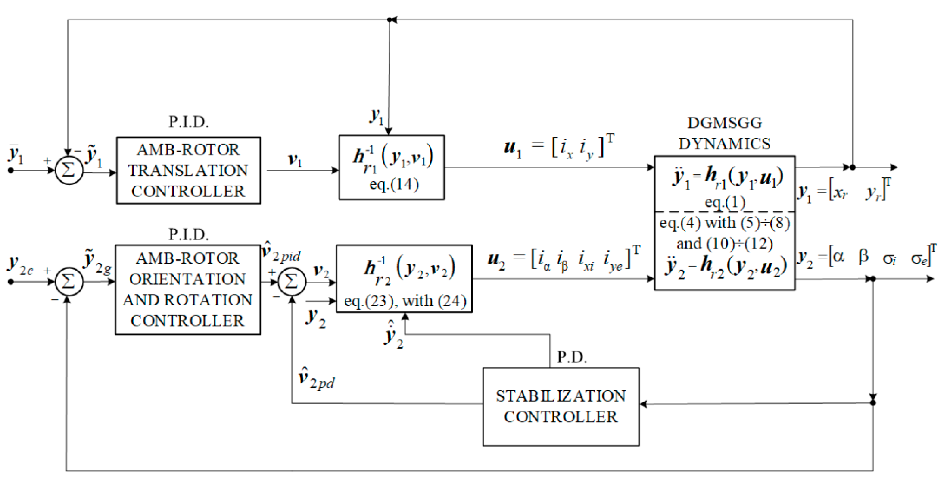
4. Structure of the DGMSGG’s Automatic Control System Based on the Dynamic Inversion Concept

DGMSGG’s automatic control system’s structure is depicted in Figure 2 and is made up of two subsystems: the subsystem for controlling the AMB–rotor’s translation and the subsystem for controlling the rotation angles of the AMB–rotor and of the gimbals.

With respect to the output vector ${\mathit{y}}_1$, the subsystem (1) has the relative degree equal to 2, because all derivatives of ${\mathit{y}}_1$ of order $i\in \left[\begin{array}{cc}0& r_i\end{array}\right)$ do not depend on ${\mathit{u}}_1$ and the derivative of the second order depends on ${\mathit{u}}_1$ [28]; ${\ddot{\mathit{y}}}_1={\mathit{h}}_{r1}(y_1,u_1)$, as shown in Figure 2.

By compensating the function ${\mathit{h}}_{r1}$ with the function ${\mathit{h}}_{r1}^{-1}$ (${\mathit{h}}_{r1}{\mathit{h}}_{r1}^{-1}\cong I_2$, where $I_2$ is the unit matrix $2\times 2$), the following equation results:

$${\ddot{\mathit{y}}}_1={\mathit{v}}_1,{\mathit{v}}_1={[v_{11}{v}_{12}]}^T={\widehat{\mathit{v}}}_{1pid}+{\ddot{\overline{\mathit{y}}}}_1,$$

(13)

and, consequently, one obtains the inverse dynamics equation of the subsystem (1)

$$\begin{array}{l}{\mathit{u}}_1={\mathit{h}}_{r1}^{-1}({\mathit{y}}_1,{\mathit{v}}_1)={\left[\begin{array}{cc}{\displaystyle \frac{2k_{xr}}{m}}& 0\\ 0& {\displaystyle \frac{2k_{yr}}{m}}\end{array}\right]}^{-1}\left\{{\mathit{v}}_1-\left[\begin{array}{cc}{\displaystyle \frac{2k_{hx}}{m}}& 0\\ 0& {\displaystyle \frac{2k_{hy}}{m}}\end{array}\right]{\mathit{y}}_1-{\mathit{g}}_0\right\}\\ \end{array}.$$

(14)

To deduce the relative degrees of the dynamics of the subsystem (which has the output vector ${\mathit{y}}_2$) in relation to its variables $\left(y_{2i},i=\overline{1,4}\right)$, the theory of differential geometry (Lie derivatives, as presented in Appendix A) is used [18]. Thus, the derivative with respect to time of the variable $y_{2i}$ is calculated as:

$$\begin{array}{ll}{\dot{y}}_{2i}={\dot{h}}_i(\mathit{x})={\displaystyle \frac{\partial h_i(\mathit{x})}{\partial \mathit{x}}}\dot{\mathit{x}}& \stackrel{(7)}{=}{\displaystyle \frac{\partial h_i}{\partial \mathit{x}}}[\mathit{f}(\mathit{x})+\mathit{g}(\mathit{x}){\mathit{u}}_2]={\displaystyle \frac{\partial h_i}{\partial \mathit{x}}}\mathit{f}(\mathit{x})+{\displaystyle \frac{\partial h_i}{\partial \mathit{x}}}\mathit{g}(\mathit{x}){\mathit{u}}_2=\\ & \stackrel{\Delta }{=}{L}_f{h}_i(\mathit{x})+\underset{j=1}{\overset{4}{\Sigma }}{L}_{gj}{h}_i(\mathit{x})u_{2j},i=\overline{1,4}.\end{array}$$

(15)

If $L_{gj}{h}_i\left(\mathit{x}\right)=0$, for $i,j=\overline{1,4}$, then we can further derive ${\dot{y}}_{2i}=L_f{h}_i(\mathit{x})=F_i(\mathit{x})$;

$$\begin{array}{ll}{\ddot{y}}_{2i}& ={\ddot{h}}_i(\mathit{x})={\displaystyle \frac{d^2{h}_i}{d{t}^2}}=h_i^{(2)}={\displaystyle \frac{d{F}_i(\mathit{x})}{dt}}={\displaystyle \frac{\partial F_i(\mathit{x})}{\partial \mathit{x}}}\dot{\mathit{x}}\stackrel{(7)}{=}{\displaystyle \frac{\partial F_i(\mathit{x})}{\partial \mathit{x}}}\cdot \\ & \cdot [\mathit{f}(\mathit{x})+\mathit{g}(\mathit{x}){\mathit{u}}_2]={\displaystyle \frac{\partial F_i(\mathit{x})}{\partial \mathit{x}}}\mathit{f}(\mathit{x})+{\displaystyle \frac{\partial F_i(\mathit{x})}{\partial \mathit{x}}}\mathit{g}(\mathit{x}){\mathit{u}}_2=\\ & =L_f{L}_f{h}_i(\mathit{x})+L_g{L}_f{h}_i(\mathit{x})\cdot {\mathit{u}}_2=L_f^2{h}_i(\mathit{x})+\underset{j=1}{\overset{4}{\Sigma }}{L}_{gj}{L}_f{h}_i(\mathit{x})\cdot u_{2j}.\end{array}$$

(16)

Thus,

$${\ddot{y}}_{2i}=L_f^2{h}_i(\mathit{x})=\underset{j=1}{\overset{4}{\Sigma }}{L}_{gj}{L}_f{h}_i(\mathit{x})\cdot u_{2j},i=\overline{1,4;}$$

(17)

According to hypothesis 1 in [28], the relative degree of the subsystem with respect to each variable $y_{2i},i=\overline{1,4}$ is equal to 2. From (17), the resulting formulas are

$$L_f^2{h}_i(\mathit{x})=L_f(L_f{h}_i(\mathit{x}))={\displaystyle \frac{\partial }{\partial \mathit{x}}}(F_i(\mathit{x}))\mathit{f}(\mathit{x})={\displaystyle \frac{\partial }{\partial \mathit{x}}}(L_f{h}_i(\mathit{x}))\mathit{f}(\mathit{x}),i=\overline{1,4},$$

(18)

$$L_{gj}{L}_f{h}_i(\mathit{x})=L_{gj}(L_f{h}_i(\mathit{x}))={\displaystyle \frac{\partial }{\partial \mathit{x}}}(F_i(\mathit{x})){\mathit{g}}_j(\mathit{x})={\displaystyle \frac{\partial }{\partial \mathit{x}}}(L_f{h}_i(\mathit{x})){\mathit{g}}_j(\mathit{x}),i=\overline{1,4}.$$

(19)

Combining Equation (17), $i=\overline{1,4}$, one obtains the matrix–vector equation

$${\ddot{\mathit{y}}}_2={\mathit{h}}_{r2}({\mathit{y}}_2,{\mathit{v}}_2)=\mathit{A}(\mathit{x})+\mathit{B}(\mathit{x}){\mathit{u}}_2,{\ddot{\mathit{y}}}_2={\mathit{v}}_2,$$

(20)

where the matrices $\mathit{A}\left(\mathit{x}\right)$ and $\mathit{B}\left(\mathit{x}\right)$ have the following forms:

$$\mathit{A}(\mathit{x})={[A_1(\mathit{x})A_2(\mathit{x})A_3(\mathit{x})A_4(\mathit{x})]}^T={[L_f^2{h}_1(\mathit{x})L_f^2{h}_2(\mathit{x})L_f^2{h}_3(\mathit{x})L_f^2{h}_4(\mathit{x})]}^T,$$

(21)

$$\mathit{B}(\mathit{x})=\left[\begin{array}{cccc}{L}_{g1}{L}_f{h}_1(\mathit{x})& L_{g2}{L}_f{h}_1(\mathit{x})& L_{g3}{L}_f{h}_1(\mathit{x})& L_{g4}{L}_f{h}_1(\mathit{x})\\ L_{g1}{L}_f{h}_2(\mathit{x})& L_{g2}{L}_f{h}_2(\mathit{x})& L_{g3}{L}_f{h}_2(\mathit{x})& L_{g4}{L}_f{h}_2(\mathit{x})\\ L_{g1}{L}_f{h}_3(\mathit{x})& L_{g2}{L}_f{h}_3(\mathit{x})& L_{g3}{L}_f{h}_3(\mathit{x})& L_{g4}{L}_f{h}_3(\mathit{x})\\ L_{g1}{L}_f{h}_4(\mathit{x})& L_{g2}{L}_f{h}_4(\mathit{x})& L_{g3}{L}_f{h}_4(\mathit{x})& L_{g4}{L}_f{h}_4(\mathit{x})\end{array}\right].$$

(22)

Consequently, the inverse dynamics of the subsystem (4) are described by:

$${\mathit{u}}_2={\mathit{h}}_{r2}^{-1}({\mathit{y}}_2,{\mathit{v}}_2)={\mathit{B}}^{-1}(\mathit{x})[{\mathit{v}}_2-{\mathit{A}}_c(\mathit{x})],{\mathit{v}}_2=[v_{21}{v}_{22}{v}_{23}{v}_{24}{]}^T.$$

(23)

After performing the calculations (given in the Appendix A), one obtains the matrices

$$\mathit{A}(\mathit{x})=\left[\begin{array}{c}{f}_2\left(\mathit{x}\right)\\ f_4\left(\mathit{x}\right)\\ f_6\left(\mathit{x}\right)\\ f_8\left(\mathit{x}\right)\end{array}\right],{\mathit{A}}_c(\mathit{x})=\left[\begin{array}{c}{\widehat{f}}_2\left(\mathit{x}\right)\\ {\widehat{f}}_4\left(\mathit{x}\right)\\ {\widehat{f}}_6\left(\mathit{x}\right)\\ {\widehat{f}}_8\left(\mathit{x}\right)\end{array}\right],\mathit{B}(\mathit{x})=\left[\begin{array}{cccc}{g}_{12}& 0& g_{32}& g_{42}\\ 0& g_{24}& g_{34}& g_{44}\\ g_{16}& 0& g_{36}& g_{46}\\ 0& g_{28}& g_{38}& g_{48}\end{array}\right],$$

(24)

where the terms ${\widehat{f}}_2,{\widehat{f}}_4,{\widehat{f}}_6,{\widehat{f}}_8$ have the expressions in (10). The state variables $x_2$, $x_4$, $x_6$, and $x_8$ were replaced by their estimated values ${\widehat{x}}_2,{\widehat{x}}_4,{\widehat{x}}_6$, and ${\widehat{x}}_8$, components of the estimated vector ${\widehat{\dot{\mathit{y}}}}_2$ (see Formula (36) and Figure 3a).

For the stabilization regime, using the concept of dynamic inversion, the dynamic compensator 2 and the linear observer 2 were designed. The second-order reference mode was chosen equal to the relative degree of the subsystem with the output vector ${\mathit{y}}_2$. This model provides both ${\overline{\mathit{y}}}_2$ and the derivatives ${\dot{\overline{\mathit{y}}}}_2$ and ${\ddot{\overline{\mathit{y}}}}_2$; in a state of equilibrium, one has obtained ${\mathit{y}}_2={\overline{\mathit{y}}}_2$, ${\dot{\mathit{y}}}_2={\dot{\overline{\mathit{y}}}}_2$, ${\ddot{\mathit{y}}}_2={\ddot{\overline{\mathit{y}}}}_2$. Furthermore, the orientation controller and the linear observer 3 were designed.

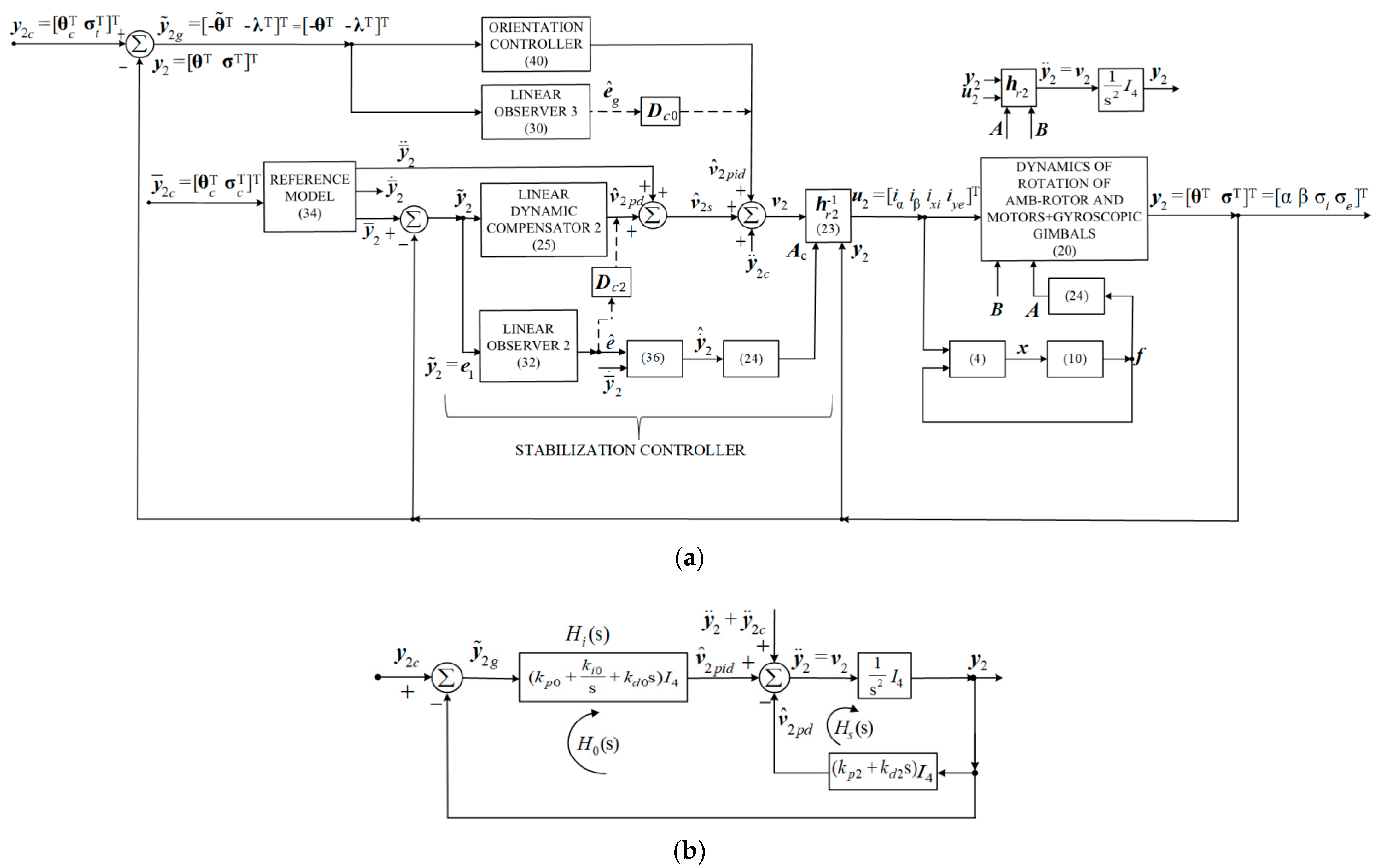
5. The Design of DGMSGG’s Automatic Control Subsystems

The structure and the design of the subsystems in Figure 2, for the AMB–rotor translation vector control, are given in [15]. The structure of the subsystem in Figure 2, for the control of AMB–rotors and gimbals’ rotation vector, is depicted in Figure 3a.

A linear dynamic compensator of P.D.-type was chosen, whose transfer matrix has the form

$$H_{cd}(s)=(K_{p2}+K_{d2}s)I_4,K_{p2}=k_{p2}{I}_4,K_{d2}=k_{d2}{I}_4,$$

(25)

where $I_4$ is the unit matrix ($4\times 4$). Taking into account the compensation of the function ${\mathit{h}}_{r2}({\mathit{y}}_2,{\mathit{u}}_2)$ by the function ${\mathit{h}}_{r2}^{-1}({\mathit{y}}_2,{\mathit{v}}_2)$, the system in Figure 3a becomes linear, having the characteristic equation

$$I_4+(K_{p2}+K_{d2}s){\displaystyle \frac{1}{s^2}}=0,$$

(26)

equivalent to

$$s^2+k_{d2}s+k_{p2}=0;$$

(27)

the coefficients $k_{p2}$ and $k_{d2}$ are calculated considering the roots of Equation (27).

According to Figure 3a

$${\mathit{v}}_2={\widehat{\mathit{v}}}_{2pd}+{\ddot{\overline{\mathit{y}}}}_2+{\widehat{\mathit{v}}}_{2pid}=K_{p2}{\tilde{\mathit{y}}}_2+K_{d2}{\dot{\tilde{\mathit{y}}}}_2+\ddot{\overline{\mathit{y}}}+{\widehat{\mathit{v}}}_{2pid},$$

(28)

The equation ${\ddot{\mathit{y}}}_2={\mathit{v}}_2$ becomes

$${\ddot{\tilde{\mathit{y}}}}_2=-K_{p2}{\tilde{\mathit{y}}}_2-K_{d2}\dot{\tilde{\mathit{y}}}-{\widehat{\mathit{v}}}_{2pid}.$$

(29)

Considering that $\mathit{e}$ is the state vector of the subsystem, which has the input ${\widehat{\mathit{v}}}_{2pid}$ and the output ${\tilde{\mathit{y}}}_2$, one obtains

$$\mathit{e}={\left[{\mathit{e}}_1^T{\mathit{e}}_2^T\right]}^T=\left[{\tilde{\mathit{y}}}_2^T{\dot{\tilde{\mathit{y}}}}_2^T\right],{\mathit{e}}_1={\tilde{\mathit{y}}}_2={[\tilde{\alpha }\tilde{\beta }{\tilde{\sigma }}_i{\tilde{\sigma }}_e]}^T,{\mathit{e}}_2={\dot{\tilde{\mathit{y}}}}_2={[\dot{\tilde{\alpha }}\dot{\tilde{\beta }}{\dot{\tilde{\sigma }}}_i{\dot{\tilde{\sigma }}}_e]}^T,$$

(30)

and the state equation is

$$\dot{\mathit{e}}=A_2\mathit{e}+B_2{\widehat{\mathit{v}}}_{2pid},$$

(31)

with

$$A_2=\left[\begin{array}{cc}{0}_{4\times 4}& I_4\\ -K_{p2}& -K_{d2}\end{array}\right],B_2=\left[\begin{array}{c}{0}_{4\times 4}\\ -I_4\end{array}\right].$$

(32)

The equation of the linear state observer 2 is:

$$\dot{\widehat{\mathit{e}}}={\overline{A}}_2\widehat{\mathit{e}}+L_2{\tilde{\mathit{y}}}_2,{\overline{A}}_2=A_2-L_2{C}_2,C_2=\left[I_4{0}_{4\times 4}\right];$$

(33)

the observer’s amplification matrix $L_2$ is calculated from the condition that the eigenvalues of the matrix ${\overline{A}}_2$ must be located in the left complex semiplane.

To avoid the need for additional sensors, the control law ${\widehat{\mathit{v}}}_{2pd}$ is calculated with the formula

$${\widehat{\mathit{v}}}_{2pd}=D_{c2}\widehat{\mathit{e}},D_{c2}=[K_{p2}{K}_{d2}].$$

(34)

The reference model is described by the transfer matrix:

$$H_m(s)={\displaystyle \frac{{\omega }_{r0}^2}{s^2+2\xi {\omega }_{r0}+{\omega }_{r0}^2}}{I}_4,$$

(35)

with ${\xi }_0=0.7$ and ${\omega }_{r0}=2.5$ rad/s.

In Equation (23) (considering the formulas in (24)), instead of the vector ${\dot{\mathit{y}}}_2$ (whose components are used for the calculation of the functions ${\widehat{f}}_2,{\widehat{f}}_4,{\widehat{f}}_6,{\widehat{f}}_8$), the estimated vector is introduced

$${\widehat{\dot{\mathit{y}}}}_2={\left[{\widehat{x}}_2{\widehat{x}}_4{\widehat{x}}_6{\widehat{x}}_8\right]}^T={[\widehat{\dot{\alpha }}\widehat{\dot{\beta }}{\widehat{\dot{\sigma }}}_i{\widehat{\dot{\sigma }}}_e]}^T.$$

(36)

In order not to use additional sensors for the variables $x_2,x_4,x_6$, and $x_8$, it is considered:

$${\widehat{\dot{\mathit{y}}}}_2={\dot{\overline{\mathit{y}}}}_2-{\widehat{\dot{\tilde{\mathit{y}}}}}_2={\dot{\overline{\mathit{y}}}}_2-{\widehat{\mathit{e}}}_2,$$

(37)

where ${\widehat{\mathit{e}}}_2$ is the second component of the vector $\widehat{\mathit{e}}$ $\left(\widehat{\mathit{e}}={\left[\begin{array}{cc}{\widehat{\mathit{e}}}_1^{\mathrm{T}}& {\widehat{\mathit{e}}}_2^{\mathrm{T}}\end{array}\right]}^{\mathrm{T}}\right)$, while the vector ${\dot{\overline{\mathit{y}}}}_2$ is provided by the reference model.

In Figure 3a, one has used the notations:

$${\overline{\mathit{y}}}_{2c}={\left[{\mathit{\theta }}_c{\mathit{\sigma }}_c\right]}^T,{\mathit{\theta }}_c={\left[{\alpha }_c{\beta }_c\right]}^T={\left[00\right]}^T,{\mathit{\sigma }}_c={\left[{\sigma }_{ic}{\sigma }_{ec}\right]}^T={\left[00\right]}^T,$$

(38)

$$\begin{array}{l}{\mathit{y}}_{2c}={\left[{\mathit{\theta }}_c{\mathit{\sigma }}_t\right]}^T,{\mathit{\sigma }}_t={\left[{\sigma }_{ti}{\sigma }_{te}\right]}^T={\left[00\right]}^T,\mathit{\sigma }={\left[{\sigma }_i{\sigma }_e\right]}^T,\\ \mathit{\lambda }={\left[{\lambda }_i{\lambda }_e\right]}^T,\tilde{\mathit{\theta }}={\mathit{\theta }}_c-\mathit{\theta }={\left[{\alpha }_c-\alpha {\beta }_c-\beta \right]}^T,\end{array}$$

(39)

expressions that are consistent with Figure 1b; when equilibrium was achieved, the line of sight overlaps the guidance line, which means

$$\mathit{\sigma }={\mathit{\sigma }}_t,\mathit{\lambda }={\left[00\right]}^T;$$

(40)

the angular (kinetic) momentum vector ${\overrightarrow{\mathit{K}}}_0$ overlaps the guidance line.

In Figure 3b, the block diagram of the linear subsystem for ${\mathit{h}}_{r2}^{-1}{\mathit{h}}_{r2}\cong I_4$ is depicted.

The guidance controller is chosen as P.I.D.-type, having the output

$$\begin{array}{l}{\widehat{\mathit{v}}}_{2pid}=K_{i0}\int {\tilde{\mathit{y}}}_{2g}+K_{po}{\tilde{\mathit{y}}}_{2g}+K_{do}{\tilde{\mathit{y}}}_{2g},K_{i0}=k_{i0}{I}_4,K_{p0}=k_{p0}{I}_4,K_{d0}=k_{d0}{I}_4\\ {\widehat{\mathit{v}}}_{2pid}=D_{c0}{\tilde{\mathit{y}}}_{2g},D_{c0}=\left[K_{i0}{K}_{p0}{K}_{d0}\right]\end{array}.$$

(41)

The transfer matrix of the inner contour is

$$H_s(s)={\displaystyle \frac{1}{s^2+k_{d2}s+k_p}}{I}_4,$$

(42)

while one of the outer contours is

$$H_o(s)={\displaystyle \frac{k_{d0}{s}^2+k_{p0}s+k_{i0}}{s^2+k_{d}s+k_{p}s+k_{i0}}}{I}_4,$$

(43)

with $k_d=k_{d0}+k_{d2}$ and $k_p=k_{p0}+k_{p2}$.

To calculate the coefficients $k_{i0}$ and $k_{p0}$, the condition is imposed that the roots of the following characteristic equation are located in the left complex semiplane:

$$s^3+k_d{s}^2+k_p+k_{i0}=0.$$

(44)

Furthermore, the linear state observatory 3 is designed. According to Figure 3a ${\ddot{\mathit{y}}}_2\approx {\mathit{v}}_2$ and, according to Figure 3a,

$${\mathit{v}}_2={\widehat{\mathit{v}}}_{2pid}+{\widehat{\mathit{v}}}_{2s}+{\ddot{\mathit{y}}}_{2c}=K_{i0}{\displaystyle \int {\tilde{\mathit{y}}}_{2g}}+K_{p0}{\tilde{\mathit{y}}}_{2g}+K_{d0}{\dot{\tilde{\mathit{y}}}}_{2g}+{\widehat{\mathit{v}}}_{2s}+{\ddot{\mathit{y}}}_{2c};$$

(45)

the vector ${\ddot{\mathit{y}}}_{2c}={\left[\begin{array}{cccc}0& 0& 0& 0\end{array}\right]}^{\mathrm{T}}$ was introduced to ensure the convergence ${\ddot{\mathit{y}}}_2={\ddot{\mathit{y}}}_{2c}$. So

$${\ddot{\mathit{y}}}_2={\mathit{v}}_2=K_{i0}{\displaystyle \int {\tilde{\mathit{y}}}_{2g}}+K_{p0}{\tilde{\mathit{y}}}_{2g}+K_{d0}{\dot{\tilde{\mathit{y}}}}_{2g}+{\widehat{\mathit{v}}}_{2s}+{\ddot{\mathit{y}}}_{2c},$$

(46)

equivalent to

$${\ddot{\tilde{\mathit{y}}}}_{2g}=-K_{i0}{\displaystyle \int {\tilde{\mathit{y}}}_{2g}}-K_{p0}{\tilde{\mathit{y}}}_{2g}-K_{d0}{\dot{\tilde{\mathit{y}}}}_{2g}-{\widehat{\mathit{v}}}_{2s}.$$

(47)

Considering that ${\mathit{e}}_g$ is the state vector of the subsystem with the input ${\widehat{\mathit{v}}}_{2s}$ and the output ${\tilde{\mathit{y}}}_{2g}$;${\mathit{e}}_g={\left[\begin{array}{ccc}{\mathit{e}}_{g1}^{\mathrm{T}}& {\mathit{e}}_{g2}^{\mathrm{T}}& {\mathit{e}}_{g3}^{\mathrm{T}}\end{array}\right]}^{\mathrm{T}}$, ${\mathit{e}}_{g1}={\displaystyle \int {\tilde{y}}_{2g}}$, ${\mathit{e}}_{g2}={\tilde{y}}_{2g}$,${\mathit{e}}_{g3}={\dot{\tilde{y}}}_{2g}$. The state equations of this subsystem are

$$\begin{array}{l}{\dot{\mathit{e}}}_{g1}={\mathit{e}}_{g2},\\ {\dot{\mathit{e}}}_{g2}={\mathit{e}}_{g3},\\ {\dot{\mathit{e}}}_{g3}=-K_{i0}{\mathit{e}}_{g1}-K_{p0}{\mathit{e}}_{g2}-K_{d0}{\mathit{e}}_{g3}-{\widehat{\mathit{v}}}_{2s},\end{array}$$

(48)

respectively, the vector state equation is

$${\dot{\mathit{e}}}_g=A_3{\mathit{e}}_g+B_3{\widehat{\mathit{v}}}_{2s},$$

(49)

where

$$A_3=\left[\begin{array}{ccc}{0}_{4\times 4}& I_4& 0_{4\times 4}\\ 0_{4\times 4}& 0_{4\times 4}& I_4\\ -K_{i0}& -K_{p0}& -K_{d0}\end{array}\right],B_3=\left[\begin{array}{c}{0}_{4\times 4}\\ 0_{4\times 4}\\ -I_4\end{array}\right].$$

(50)

Since there are no sensors to measure the components of the vector ${\dot{\tilde{\mathit{y}}}}_{2g}={\left[\begin{array}{cccc}-\dot{\alpha }& -\dot{\beta }& -{\dot{\lambda }}_i& -{\dot{\lambda }}_e\end{array}\right]}^{\mathrm{T}}$, the linear observer 3 is used; it is described by the state equation of the estimated vector ${\widehat{\mathit{e}}}_g$ (the estimation of the vector ${\mathit{e}}_g$)

$${\dot{\widehat{\mathit{e}}}}_g={\overline{A}}_3{\widehat{\mathit{e}}}_g+L_3{\tilde{\mathit{y}}}_{2g},$$

(51)

where ${\overline{A}}_3=A_3-L_3{C}_3$, $C_3=\left[\begin{array}{ccc}{0}_{4\times 4}& I_4& 0_{4\times 4}\end{array}\right]$. The observer’s amplification matrix $L_3$ is calculated from the condition that the matrix ${\overline{A}}_3$ has its eigenvalues located in the left complex semiplane.

According to Figure 3a,b

$$\begin{array}{ll}\mathit{\lambda }=-{\displaystyle \frac{I_2}{I_2+H_i(s)+H_s(s)I_2}}{\mathit{\sigma }}_t& =-{\displaystyle \frac{s(s^2+k_{d2}s+k_{p2})}{s^3+k_d{s}^2+k_{p}s+k_{i0}}}{I}_2{\mathit{\sigma }}_t=\\ & =-{\displaystyle \frac{(s^2+k_{d2}s+k_{p2})}{s^3+k_d{s}^2+k_{p}s+k_{i0}}}{I}_2{\dot{\mathit{\sigma }}}_t\end{array},$$

(52)

and, for a stabilized mode,

$$\mathit{\lambda }=-{\displaystyle \frac{k_{p2}}{k_{i0}}}{\dot{\mathit{\sigma }}}_t=-{\displaystyle \frac{k_{p2}}{k_{i0}}}{\mathit{\omega }}_t.$$

(53)

If the rocket guidance is performed using the parallel approach method, then ${\dot{\mathit{\sigma }}}_t={\left[\begin{array}{cc}0& 0\end{array}\right]}^{\mathrm{T}}$, and, for this purpose, signals proportional to the angles ${\lambda }_i$ and ${\lambda }_e$ are applied to the autopilot (which are the components of the $\mathit{\lambda }-$vector, provided by the target coordinator CT from the DGMSGG); ${\dot{\mathit{\sigma }}}_t={\mathit{\omega }}_t$ is the guidance line’s angular rate.

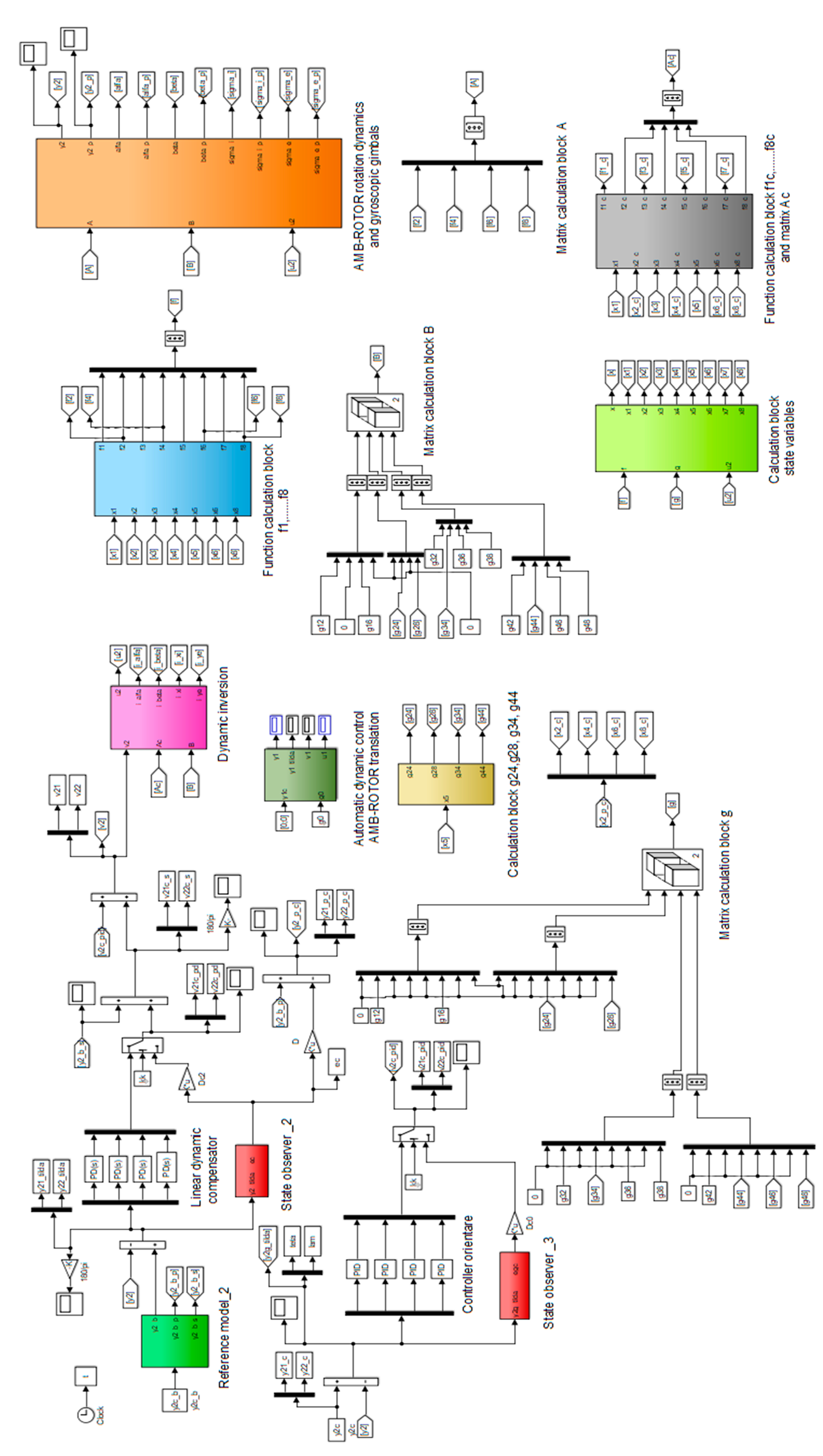
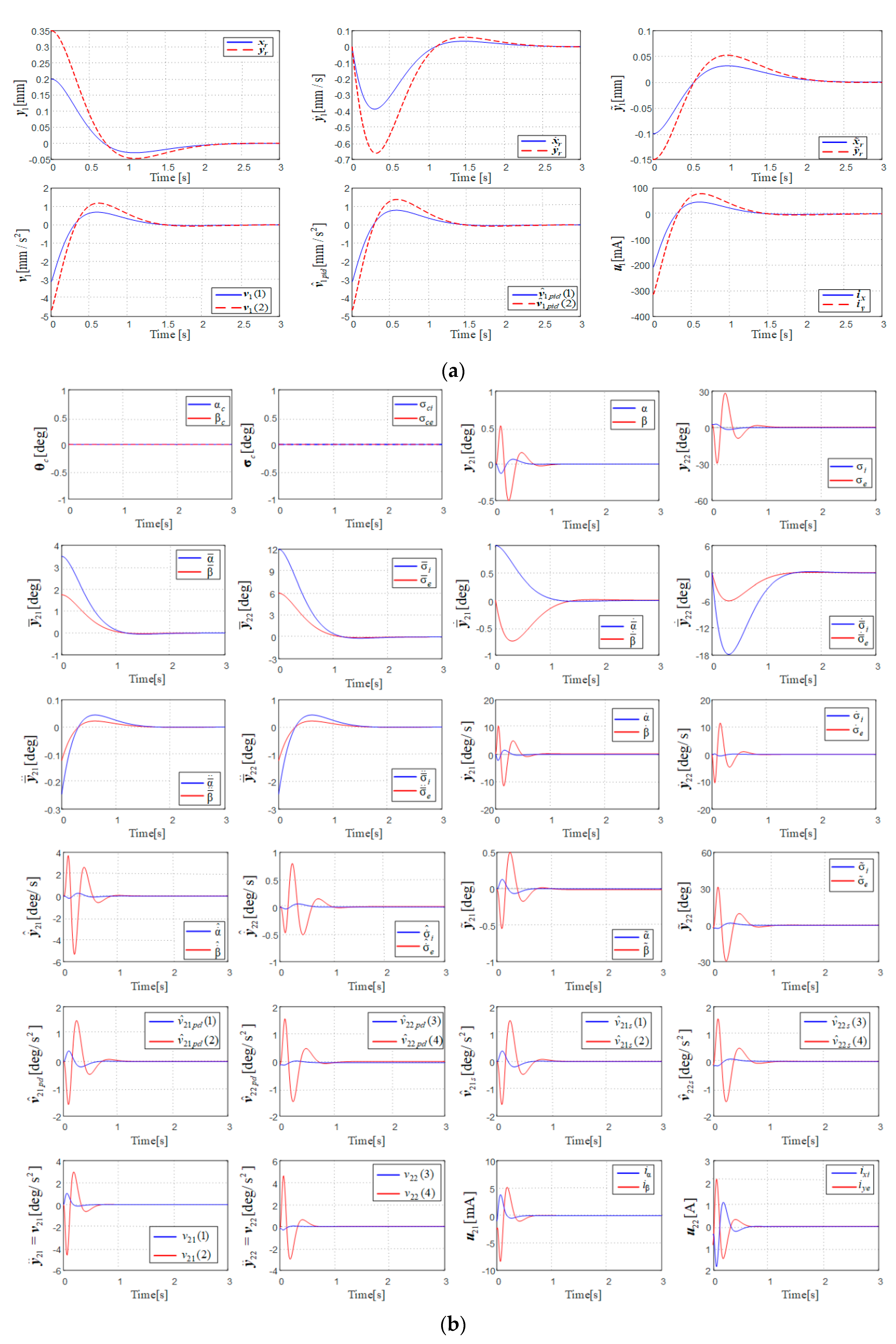
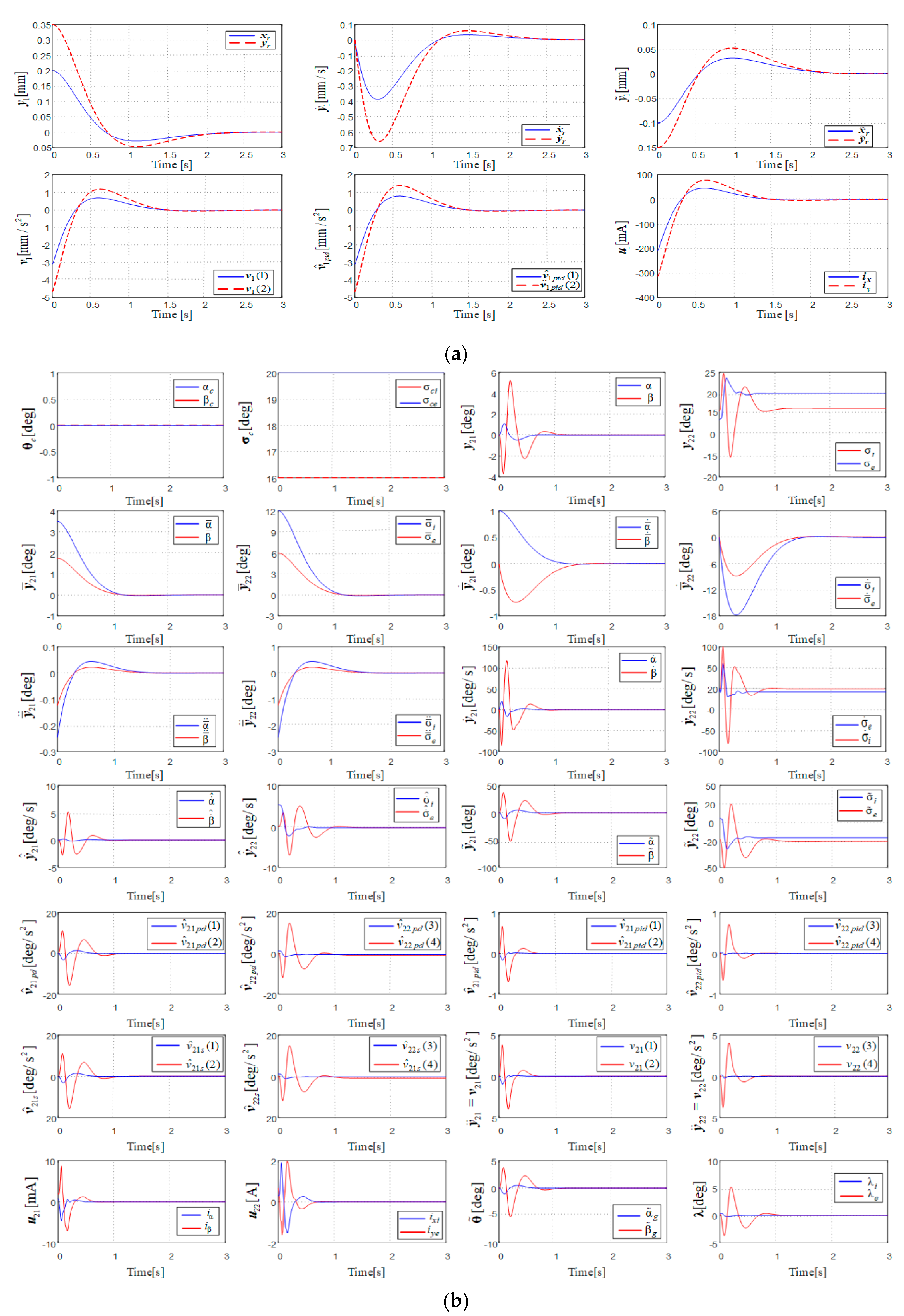
6. Results and Discussions

Starting from the nonlinear dynamic model of the gyroscopic equipment with two gimbals and an AMB–rotor, we have decoupled the subsystem describing the AMB–rotor’s dynamics of translations, described by Equation (1), from the subsystem describing the dynamics of the AMB–rotor and of the gyro gimbals, considering the fact that they are not physically interconnected. The rotation dynamics model was modified, taking into account the angular rate ${\omega }_{X_T}$ generated by the base rotations. It has resulted in the nonlinear dynamic model, described by the input state and output state Equation (4), with (5) ÷ (8), (10), and (11). The relative degrees with respect to all output variables (components of the output vectors ${\mathit{y}}_1$ and ${\mathit{y}}_2$) are equal to 2.

One has studied the dynamics of the DGMSGG through Simulink/Matlab simulations, using the following numerical values:

$$\begin{array}{l}m=2.8 \mathrm{kg},l_m=4.1\cdot {10}^{-2}\mathrm{m},l_s=6.5\cdot {10}^{-2}\mathrm{m},k_{xr}=k_{yr}=0.21\mathrm{N}/\mathrm{mA},\\ k_{hx}=0.8\mathrm{N}/\mathrm{m},k_{hx}=0.8\mathrm{N}/\mathrm{m},J_{rx}=J_{ry}=5\cdot {10}^{-2}{\mathrm{N}\times \mathrm{m}\times \mathrm{s}}^2/\mathrm{rad},\\ J_{rz}=6\cdot {10}^{-2}{\mathrm{N}\times \mathrm{m}\times \mathrm{s}}^2/\mathrm{rad}, J_{ix}=J_{iy}=5\cdot {10}^{-2}{\mathrm{N}\times \mathrm{s}}^2/\mathrm{rad},\\ J_{iz}=4\cdot {10}^{-2}{\mathrm{N}\times \mathrm{m}\times \mathrm{s}}^2/\mathrm{rad},J_{ey}=10{\mathrm{N}\times \mathrm{m}\times \mathrm{s}}^2/\mathrm{rad},k_{xi}=100 \mathrm{N}\times \mathrm{m}/\mathrm{A},\\ k_{ye}=80 \mathrm{N}\times \mathrm{m}/\mathrm{A},K_0=18\mathrm{N}\times \mathrm{m}/\mathrm{s},\alpha \left(0\right)=0.02\mathrm{rad},\\ \beta \left(0\right)=0.015\mathrm{rad},\dot{\alpha }\left(0\right)=\dot{\beta }\left(0\right)=0\mathrm{rad}/\mathrm{s},{\sigma }_i\left(0\right)=2.5\mathrm{deg}=0.43\mathrm{rad},\\ {\sigma }_e\left(0\right)=3.5\mathrm{deg}=0.061\mathrm{rad},{\dot{\sigma }}_i\left(0\right)={\dot{\sigma }}_e\left(0\right)=0\mathrm{rad}/\mathrm{s},{\overline{x}}_r\left(0\right)=1\cdot {10}^{-4}\mathrm{m},\\ {\overline{y}}_r\left(0\right)=2\cdot {10}^{-4}\mathrm{m},{\alpha }_c={\beta }_c=0\mathrm{rad}, {\dot{\sigma }}_{ic}\left(0\right)={\dot{\sigma }}_{ec}\left(0\right)=0\mathrm{rad}/\mathrm{s},\\ {\overline{\alpha }}_c\left(0\right)=1.75\cdot {10}^{-4}\mathrm{rad},{\overline{\beta }}_c\left(0\right)=1.75\cdot {10}^{-4}\mathrm{rad},\\ {\overline{\sigma }}_{ic}\left(0\right)=0.1\mathrm{rad},{\overline{\sigma }}_{ec}\left(0\right)=0.2\mathrm{rad},\\ {\sigma }_{ti}=16\mathrm{deg},{\sigma }_{te}=20\mathrm{deg},{\xi }_0=0.7,\\ w_{r0}=2.5\mathrm{rad}/\mathrm{s}.\end{array}$$

The Simulink/Matlab model (in Figure 4) was built for the system in Figure 3 and, based on it, the dynamic characteristics in Figure 5 (for the stabilization mode) and in Figure 6 (for the orientation mode) were plotted.

The first six sets of graphs are for the AMB–rotor’s translation control subsystem, which is the same for the stabilization mode (Figure 5a) as for the orientation mode (Figure 6a), this subsystem being decoupled from the one in Figure 3a.

The next sets of graphs refer to the AMB–rotor’s angular displacement control subsystem for the stabilization mode (Figure 5b) and, similarly, for the orientation mode (Figure 6b), as well as $\tilde{\mathit{\theta }}$ and $\mathit{\lambda }$ for the orientation mode (Figure 6b).

It can be mentioned that the graphs for ${\theta }_c,{\overline{\mathit{y}}}_{21},{\overline{\mathit{y}}}_{22},{\dot{\overline{\mathit{y}}}}_{21},{\dot{\overline{\mathit{y}}}}_{22},{\ddot{\overline{\mathit{y}}}}_{21}$, and ${\ddot{\overline{\mathit{y}}}}_{22}$ are the same for both operating modes because the reference model is the same for both studied modes.

All dynamic modes are fast (most have settling times under 1 s), have small overshoots, and zero static errors (${\tilde{\mathit{y}}}_1={\left[\begin{array}{cc}0& 0\end{array}\right]}^{\mathrm{T}}$, ${\tilde{\mathit{y}}}_2={\left[\begin{array}{cccc}0& 0& 0& 0\end{array}\right]}^{\mathrm{T}}$) in stabilization mode, as well as in orientation mode (${\tilde{\mathit{y}}}_1={\left[\begin{array}{cc}0& 0\end{array}\right]}^{\mathrm{T}}$, ${\tilde{\mathit{y}}}_2={\left[\begin{array}{cccc}0& 0& -{\sigma }_{ti}& -{\sigma }_{te}\end{array}\right]}^{\mathrm{T}}$ and $\tilde{\mathit{\theta }}=\mathit{\lambda }={\left[\begin{array}{cc}0& 0\end{array}\right]}^{\mathrm{T}}$).

The control (command) currents applied to the magnetic bearings’ stator coils stabilize at zero, ${\widehat{\mathit{v}}}_{pid}=-{\mathit{v}}_{pd}$ so their sum stabilizes at zero, while the components of the output vectors and their derivatives stabilize at zero in stabilization mode, respectively, ${\mathit{y}}_2\to {\left[\begin{array}{cccc}0& 0& {\sigma }_{ti}& {\sigma }_{te}\end{array}\right]}^{\mathrm{T}}$ in orientation mode.

7. Conclusions

Summarizing the above, we can specify the following elements of novelty and modernity brought by the paper:

• A new form of nonlinear dynamic model described by equations of state for the interconnected dynamics of AMB–rotor’s rotations and of gyroscopic gimbals’ rotations;
• Decoupling the dynamics of the AMB–rotor’s translations from the dynamics of its rotations and of the gimbals’ rotations;
• Determination of the nonlinear input–output vector equation, which highlights the relative degrees of the model in relation to the variables of the output vector ${\mathit{y}}_2$, using a theory of differential geometry (based on the Lie derivative calculus);
• Design of the output vector ${\mathit{y}}_2$ control structure using the dynamic inversion concept, comprising two subsystems: one for stabilization (with reference model and stabilization controller, consisting of a linear dynamic compensator of P.D.-type and linear state observer); another one for orientation (with P.I.D-type orientation controller and linear state observer);

Comparisons with the performance of other similar system structures can only be made if the same dynamic models are used, having the same numerical values of the physical parameters. The performances of the designed control structure are very close to the performances of the adaptive control structures based on neural networks designed and presented in [27,36].

References

1. Bai, J.G.; Zhang, X.Z.; Wang, L.M. A Flywheel Energy Storage System with Active Magnetic Bearings. In Proceedings of the 2012 International Conference on Future Energy, Environment and Material, Hong Kong, China, 12–13 April 2012; pp. 1124–1128. [Google Scholar]
2. Li, H.; Ning, X.; Han, B. Speed Tracking Control for Gimbal System Harmonic Drive. In Control Engineering Practice, no.58; Elsevier: Amsterdam, The Netherlands, 2017; pp. 204–213. [Google Scholar]
3. Sasaki, T.; Shimomura, T.; Schaub, H. Robust attitude control using a double-gimbal variable-speed control moment gyroscope. J. Spacecr. Rocket. 2018, 55, 1235–1247. [Google Scholar] [CrossRef]
4. Zheng, S.; Han, B. Investigations of an Integrated Angular Velocity Measurement and Attitude Control System for Spacecraft Using Magnetically Suspended Double-Gimbal CMGs. Adv. Space Res. 2013, 51, 2216–2228. [Google Scholar] [CrossRef]
5. Leeghim, H.; Kim, D. Singularity-robust control moment gyro allocation strategy for spacecraft attitude control in the presence. of disturbances. Aerosp. Sci. Technol. 2021, 119, 107178. [Google Scholar] [CrossRef]
6. Lungu, R.; Lungu, M.; Ioan, M. Determination and control of the satellites’ attitude by using a pyramidal configuration of four control moment gyros. In Proceedings of the 12th IEEE International Conference on Informatics in Control, Automation and Robotics, Colmar, France, 21–23 July 2015; pp. 448–456. [Google Scholar]
7. Ma, Z.Q.; Huang, P.F. Discrete-time sliding mode control for deployment of tethered space robot with only length and angle measurement. IEEE Trans. Aerosp. Electron. Syst. 2020, 56, 585–596. [Google Scholar] [CrossRef]
8. Schweitzer, G. Active Magnetic Bearings—Chances and Limitations. In International Center for Magnetic Bearings; EHT Zurich: Zürich, Switzerland, 2002. [Google Scholar]
9. Yue, C.; Kuman, K.D.; Shen, Q.; Gogh, C.H.; Lee, T.H. Attitude Stabilization Using Two Parallel Single-Gimbal Control Moment Gyroscopes. J. Guid. Control Dyn. 2019, 42, 1353–1364. [Google Scholar] [CrossRef]
10. Kim, H.Y.; Lee, C.W. Design and Control of Active Magnetic Bearings System with Lorentz Force-Type Axial Actuator. Mechatronics 2006, 16, 13–20. [Google Scholar] [CrossRef]
11. Yoon, H. Spacecraft Attitudne and Power Control Using Variable Control Moment Gyros. Ph.D. Thesis, Georgia Insitute of Technology, Atlanta, GA, USA, 2004. [Google Scholar]
12. Shelke, S. Controllability of Radial Magnetic Bearing. In Proceedings of the 3rd International Conference of Innovation Automation and Mechatronics Engineering, ICIAME, Vallabh Vidhyanagar, India, 5–6 February 2016; pp. 106–113. [Google Scholar]
13. Fang, J.; Sheng, S.; Han, B. AMB Vibration Control for Double-Gimbal Control Moment Gyro With High-Speed Magnetically Suspended Rotor. IEEE Trans. Mechatron. 2013, 18, 32–43. [Google Scholar] [CrossRef]
14. Lungu, R.; Ioan, M.; Lungu, M. Control of Satellites’ Attitude; Sitech Publisher: Craiova, Romania, 2017. [Google Scholar]
15. Lungu, R.; Lungu, M.; Efrim, C. Adaptive Control of DGMSCMG Using Dynamic Inversion and Neural Networks. Adv. Space Res. 2021, 68, 3478–3494. [Google Scholar] [CrossRef]
16. Su, D.; Xu, S. The Precise Control of a Double Gimbal MSCMG Based on Modal Separation and Feedback Linearization. In Proceedings of the 2013 International Conference on Electrical Machines and Systems, Busan, Republic of Korea, 26–29 October 2013; pp. 1355–1360. [Google Scholar]
17. Peng, C.; Fang, J.; Xu, S. Composite Anti-Disturbance Controller for Magnetically Suspended Control Moment Gyro Subject to Mismatched Disturbances. Nonlinear Dyn. 2015, 79, 1563–1573. [Google Scholar] [CrossRef]
18. Chen, X.; Chen, M. Precise Control of Magnetically Suspended Doble-Gimbal Control Moment Gyroscope Using Differential Geometric Decoupling Method. Chin. J. Aeronaut. 2013, 26, 1017–1028. [Google Scholar] [CrossRef]
19. Lungu, R.; Efrim, C.; Zheng, Z.; Lungu, M. Dynamic Inversion Based on Control of DGMSCMGs. Part 2: Control Arhitecture Design and Validation. In Proceedings of the IEEE International Conference on Applied and Theroretical Electricity (ICATE 2021), Craiova, Romania, 27–29 May 2021; pp. 7–12. [Google Scholar]
20. Bunryo, Y.; Satoh, S.; Shoji, Y.; Yamada, K. Feedback Attitude Control of Spacecraft Using Two Single Gimbal Control Moment Gyros. Adv. Space Res. 2021, 68, 2713–2726. [Google Scholar] [CrossRef]
21. Ahmed, J.; Bernstein, D.S. Adaptive Control of Double-Gimbal Control Moment Gyro with Unbalanced Rotor. J. Guid. Control Dyn. 2002, 25, 105–115. [Google Scholar] [CrossRef]
22. Fang, J.; Ren, Y. Decoupling Control of Magnetically Suspended Rotor in a Control Moment Gyro Based on Inverse System Method. IEEE ASME Trans. Mechatron. 2012, 17, 1133–1144. [Google Scholar] [CrossRef]
23. Lungu, M.; Lungu, R. Full-Order Observer Design for Linear Systems with Unknown Inputs. Int. J. Control 2012, 85, 1602–1615. [Google Scholar] [CrossRef]
24. Lungu, R.; Tudosie, A.-N.; Lungu, M.-A.; Crăciunoiu, N.-C. Actuators with Two Double Gimbal Magnetically Suspended Control Moment Gyros for the Attitude Control of the Satellites. Micromachines 2024, 15, 1159. [Google Scholar] [CrossRef] [PubMed]
25. Lungu, R.; Efrim, C.; Lungu, M. Gyroscopic Actuators; Sitech Publisher: Craiova, Romania, 2024. [Google Scholar]
26. Lin, F.; Chen, S.; Huang, M. Adaptive Complementary Sliding-Mode Control for Thrust Active Magnetic Bearing System. Control Eng. Pract. 2011, 19, 711–722. [Google Scholar] [CrossRef]
27. Lungu, R.; Mihai, C.-A.; Tudosie, A.-N. Guidance Gyro System with Two Gimbals and Magnetic Suspension Gyros Using Adaptive-Type Control Laws. Micromachines 2025, 16, 245. [Google Scholar] [CrossRef] [PubMed]
28. Lungu, R.; Efrim, C.; Zheng, Z.; Lungu, M. Dynamic Inversion Based on Control of DGMSCMGs. Part 1: Obtaining Nonlinear Dynamic Model. In Proceedings of the IEEE International Conference on Applied and Theroretical Electricity (ICATE 2021), Craiova, Romania, 27–29 May 2021; pp. 1–6. [Google Scholar]
29. Calise, A.J.; Hovakymyan, N.; Idan, M. Adaptive Output Control of Nonlinear Systems Using Neural Networks. Automatica 2001, 37, 1201–1211. [Google Scholar] [CrossRef]
30. Isidori, A. Nonlinear Control Systems; Springer: Berlin, Germany, 1995. [Google Scholar]
31. Lungu, R.; Lungu, M. Aircraft Landing Automatic Control; Sitech Publisher: Craiova, Romania, 2015. [Google Scholar]
32. Lungu, R. Aerospace Guidance Systems; Sitech Publisher: Craiova, Romania, 2002. [Google Scholar]
33. Lungu, R.; Mihai, C.A. Dynamic and Adaptive Control of Monoaxial GS with GAR. Part1: Obtaining the Nonlinear Dynamic Model. In Proceedings of the International Conference on Applied and Theoretical Electricity, ICATE 24, Craiova, Romania, 24–26 October 2024; pp. 1–6. [Google Scholar] [CrossRef]
34. Lungu, R.; Mihai, C.A. Dynamic and Adaptive Control of Monoaxial GS with GAR. Part 2: Control Architecture Design and Validation. In Proceedings of the International Conference on Applied and Theoretical Electricity, ICATE 24, Craiova, Romania, 24–26 October 2024; pp. 1–6. [Google Scholar] [CrossRef]
35. Mihai, C.A.; Lungu, R. Nonlinear Dynamics and Adaptive Control Using The Dynamic Inversion Concept and Neural Networks for a Guidance Gyrosystem (GG) with one Gyroscope and two Suspension Gimbals (GAR). Part 1: Obtaining the Nonlinear Dynamic Model. In Proceedings of the 26th Edition of the International Conference Scientific Research and Education in the Air Force, AFASES, Brasov, Romania, 22–24 May 2025. [Google Scholar] [CrossRef]
36. Mihai, C.A. Nonlinear Dynamics and Adaptive Control Using The Dynamic Inversion Concept and Neural Networks for a Guidance Gyrosystem (GG) with one Gyroscope and two Suspension Gimbals (GAR). Part 2: Adaptive Control Arhitecture Design and Validation. In Proceedings of the 26th Edition of the International Conference Scientific Research and Education in the Air Force, AFASES, Brasov, Romania, 22–24 May 2025. [Google Scholar] [CrossRef]
37. Lungu, M. Backstepping Control Method in Aerospace Engineering; Academia Greefswald: Rostock, Germany, 2022. [Google Scholar]
Figure 1. Frames related to the dynamic components of DGMSGG, rotation angles, angular rates, and correction moments. (a) DGMSGG’s architecture; (b) gyroscopic rotor’s centering; (c) overlapping the line of sight over the guidance line.
Actuators 14 00316 g001
Figure 2. Structure of the automatic control system of DGMSGG.
Actuators 14 00316 g002
Figure 3. Structure of the automatic control system of the AMB—rotor vector and gyroscopic gimbals: (a) complete block diagram; (b) block diagram of the linear subsystem.
Actuators 14 00316 g003
Figure 4. Simulink/Matlab model of DGMSGG.
Actuators 14 00316 g004
Figure 5. Dynamic characteristics of DGMSGG for the stabilization mode. (a) for the AMB–rotor’s translation control subsystem; (b) for the AMB–rotor’s angular displacement control subsystem for the stabilization mode.
Actuators 14 00316 g005
Figure 6. Dynamic characteristics of DGMSGG for the orientation mode. (a) for the AMB–rotor’s translation control subsystem; (b) for the AMB–rotor’s angular displacement control subsystem for the orientation mode.
Actuators 14 00316 g006
Disclaimer/Publisher’s Note: The statements, opinions and data contained in all publications are solely those of the individual author(s) and contributor(s) and not of MDPI and/or the editor(s). MDPI and/or the editor(s) disclaim responsibility for any injury to people or property resulting from any ideas, methods, instructions or products referred to in the content.