1. Introduction
Autonomous race driving represents a specialized yet critical subset of general autonomous driving tasks, distinguished by its extreme performance requirements, including precision control at high speeds and deliberate operation at vehicle dynamics limits. While these requirements differ markedly from conventional urban driving scenarios that prioritize passenger comfort and regulatory compliance, the advanced control strategies developed for racing, such as maneuvering at the limits of tire–road friction and split-second overtaking decisions, directly inform safety-critical applications in general autonomous driving, particularly in extreme scenarios like emergency obstacle evasion. This dual relevance, combining both theoretical challenges in control systems and practical applications in vehicle safety, has made autonomous racing an active area of research in academia and industry [
1,
2,
3].
The objective of autonomous racing is to complete laps as fast as possible. It requires the vehicle to operate at high speeds while maintaining safety and stability. To address this challenging driving task, numerous advanced control strategies have been proposed for autonomous race driving, including classical control [
4,
5,
6,
7,
8], learning-based intelligent control [
9,
10], and so on. Among these strategies, classical control methods basically focus on known path tracking. For example, Viadero-Monasterio et al. [
11] proposed an event-triggered LPV path tracking controller that improves safety, comfort, and communication efficiency under network delays. In contrast, reinforcement learning (RL) [
12] offers distinct advantages by automatically learning optimal policies through environmental interaction while handling high-dimensional states and continuous actions. This makes RL particularly suitable for mastering the extreme control challenges in autonomous race driving, ranging from precise friction-limit handling to competitive overtaking maneuvers.
Early RL-based approaches focused on establishing baseline capabilities. Jaritz et al. [
13] pioneered an end-to-end RL framework that directly mapped sensory inputs to control outputs, establishing foundational techniques for high-speed racing scenarios. Building upon this direct mapping approach, Hell et al. [
14] later developed a specialized LiDAR-only observation method with strong generalization capabilities across unfamiliar tracks, advancing sensor-specific implementations for practical racing applications. As the field progressed, researchers developed increasingly sophisticated techniques to refine control performance. Zhang et al. [
15] introduced a residual policy learning framework that enhanced baseline controllers through iterative experience, improving adaptability to dynamic racing conditions. This advancement in policy refinement contributed to the broader goal of achieving superhuman performance, which was later demonstrated by Fuchs et al. [
16], whose RL agent successfully surpassed human expert lap times in simulation environments. In addition, Evans et al. [
17] conducted comprehensive comparisons of various RL architectures for controlling autonomous racing vehicles, providing valuable insights into effective algorithm selection for different racing scenarios.
While high performance is the primary goal in autonomous racing, ensuring safety during both training and deployment presents a critical challenge. To address safety challenges in autonomous racing, researchers have developed many approaches focusing on different aspects of the problem. At the fundamental level of vehicle handling limits, Wang et al. [
18] introduced an action mapping (AM) mechanism combined with RL that enables vehicles to safely operate at friction boundaries while maximizing handling capability, effectively preventing instability during high-speed maneuvers. In parallel, Gottschalk et al. [
19] proposed a hybrid and hierarchical approach that integrates classical optimal control for system dynamics with RL for collision avoidance, leveraging surrogate models to accelerate training and achieve real-time control for dynamic overtaking in autonomous racing. Building upon basic vehicle control safety, researchers have addressed the challenge of dynamic uncertainties in racing environments. Niu et al. [
20] leveraged adversarial learning within an RL framework to bridge the dynamics gap, achieving remarkable safety by eliminating violations during training. Complementing this approach, Liu et al. [
21] enhanced policy robustness through a Sequential Actor–Critic architecture that leverages historical trajectory information, significantly improving learning efficiency and stability during high-speed maneuvers. Chen et al. [
22] integrated Hamilton–Jacobi (HJ) reachability theory into RL-based control algorithms to provide enhanced safety guarantees while maintaining competitive racing speeds. Extending this approach, Stachowicz et al. [
23] developed risk-sensitive control methods that explicitly quantify and balance performance objectives against safety constraints in high-speed racing scenarios.
The above methods are basically deployed on simulation platforms [
24,
25]. To address the practical challenges of real-world implementation, Cai et al. [
26] developed an innovative approach combining imitation learning (IL) with RL for vision-based autonomous racing. Their method effectively overcomes the limitations of traditional approaches that are either computationally intensive or sensitive to environmental variations, while also addressing the sample efficiency and safety trade-offs inherent in pure IL or RL implementations.
As autonomous control of single vehicles has achieved significant progress, research focus has shifted toward competitive racing scenarios that require complex multi-car interactions. A curriculum-based RL method that systematically increases task difficulty during training is proposed in [
27]. This approach strategically introduces competitive elements only after basic driving skills are mastered, enabling more efficient learning of complex behaviors. To address the collision avoidance issue in competitive scenarios, Yuan et al. [
28] established an initial hierarchical collision avoidance framework that effectively reduced collisions but encountered scalability limitations as opponent numbers increased. Addressing these limitations, Thakkar et al. [
29] advanced the field with an end-to-end RL architecture incorporating attention mechanisms to dynamically prioritize relevant opponent vehicles, significantly improving performance in densely contested racing environments. Notably, Wurman et al. [
30] developed Gran Turismo Sophy, a deep RL agent that achieved championship-level performance in a commercial racing simulator, demonstrating both high speed and tactical behaviors such as overtaking and blocking. Beyond algorithmic advances, observation space design remains a critical challenge in competitive racing environments. The approach in [
31] incorporates sensor data from vehicle-mounted LiDARs or cameras, resulting in high-dimensional observation spaces that can challenge RL algorithm learning efficiency, particularly in complex racing scenarios with multiple vehicles. These high-dimensional representations provide rich environmental information but require substantial computational resources and may introduce latency in real-time control systems. In contrast, approaches in [
27,
28,
29] utilize lower-dimensional observation spaces primarily consisting of vehicle pose, motion states, and limited track data from the car’s forward view. While computationally more efficient, these approaches often inadequately represent opponent vehicles within the observation space, limiting their effectiveness in competitive racing environments.
In summary, despite the significant progress made in the above works, the current literature still faces the following common challenges:
Limited adaptability to dynamic and competitive scenarios: Many classical and RL-based methods are primarily validated in simplified or single-vehicle settings, lacking robustness in highly dynamic racing scenarios with multiple opponent vehicles.
Safety–performance trade-off: While some methods provide safety guarantees, they may sacrifice racing performance, or vice versa. Achieving both high safety and high performance in aggressive racing remains challenging.
Insufficient handling of variable and high-dimensional observations: Existing approaches often struggle with efficiently processing variable-sized or high-dimensional sensory data, especially when the number and position of opponents change rapidly.
These challenges motivate the integrated framework proposed in this paper, which aims to enhance adaptability, observation processing, safety, and sample efficiency in competitive autonomous racing.
In this paper, we focus on the challenge of developing high-speed autonomous racing under dynamic and competitive scenarios, where safety constraints and opponent interactions must be simultaneously addressed. The key difficulties include (1) maintaining vehicle stability near the traction limits during high-speed maneuvers; (2) efficiently processing variable-dimensional observations when opponents enter/exit the field of view; (3) ensuring safe exploration during RL training to avoid catastrophic failures. To address these challenges, we propose an integrated RL framework that combines state mapping, action mapping, and safe exploration guidance to achieve both performance and safety. The three key innovations of this work are summarized as follows:
A state mapping mechanism that dynamically transforms raw track observations into a consistent representation space, enabling seamless policy transfer between different racing scenarios.
An action mapping technique that rigorously enforces physical traction constraints while maximizing the vehicle’s handling capabilities.
A safe exploration guidance method that combines conservative controllers with RL policies, significantly reducing off-track incidents during training.
The remainder of this paper is structured as follows:
Section 2 presents the vehicle dynamics model that forms the foundation of our racing environment.
Section 3 formulates the autonomous racing task as a Markov Decision Process (MDP).
Section 4,
Section 5 and
Section 6, respectively, elaborate on three key methodological contributions: the state mapping approach for dynamic environment representation (
Section 4), the action mapping mechanism for traction constraint enforcement (
Section 5), and the safe exploration guidance framework (
Section 6).
Section 7 details the implementation of the proposed RL framework. Comprehensive experimental results, including both time trial and competitive racing scenarios across multiple track configurations, are presented and analyzed in
Section 8. Finally,
Section 9 concludes the paper and outlines directions for future research.
2. Vehicle Model
To characterize the vehicle’s kinematic and dynamic behavior, we employ the single-track vehicle model, which has been extensively validated in vehicle handling research [
32,
33]. As depicted in
Figure 1, this simplified representation consolidates the front and rear wheels into single virtual wheels positioned at each axle’s centerline. The complete nomenclature is detailed in
Table 1. The model incorporates several simplifying assumptions: (1) negligible longitudinal and lateral load transfer effects; (2) uniform road–tire friction characteristics; and (3) planar motion on a flat surface. Under these assumptions, the vehicle dynamics naturally decouple into distinct longitudinal (acceleration/deceleration) and lateral (steering) components for analytical convenience.
The longitudinal model of the vehicle can be derived from the analysis of longitudinal forces:
where
m is the total mass of the vehicle,
is the longitudinal tire force, and
is the longitudinal frictional resistance. The longitudinal tire force can take two forms: driving force and braking force. In this work, we consider a vehicle driven by an electric motor, whose torque output characteristics are divided into two regions within the range from zero speed to maximum speed: the constant torque region and the constant power region. When the motor speed
is less than the base speed
of the motor, the motor operates in the constant torque region, where its output torque is proportional to the motor control signal and can deliver the maximum torque. When the motor speed
exceeds the base speed
, the motor operates in the constant power region, and the output torque is limited by the maximum power
, preventing it from maintaining the maximum torque. Combining these two cases, the driving force
of the vehicle is expressed as
where
is the torque coefficient of the motor,
is the radius of the wheel, and
is the normalized motor control signal. The braking force
is generated by the vehicle’s braking system and acts on all wheels. Assuming the braking force is proportional to the braking control signal, we have
where
is the braking force coefficient and
is the braking control signal. Since in normal conditions, acceleration and braking signals should not be input simultaneously, these two signals can be combined into one single longitudinal control signal
.
indicates maximum acceleration command, and
indicates maximum braking force command.
The longitudinal frictional resistance
is opposite to the vehicle’s direction of motion and is mainly composed of two parts: the aerodynamic drag
and the tire rolling resistance
. The equivalent aerodynamic drag of the vehicle in a windless environment is expressed as
where
is the air density,
is the vehicle’s aerodynamic drag coefficient, and
is the vehicle’s frontal area. The vehicle’s tire rolling resistance is approximately proportional to the vertical load on the tires, which is expressed as
where
is the rolling resistance coefficient and
g is the acceleration due to gravity.
The lateral and rotational dynamics of the vehicle can be described by establishing force equilibrium along the lateral direction and moment equilibrium about the vertical axis, expressed as
where
is the vehicle’s yaw moment of inertia;
and
represent the lateral tire forces at the front and rear axles, respectively. The tire forces are modeled using the Magic Formula tire model, with a detailed derivation available in [
34].
The front wheel steering angle is driven by the electric power-assisted steering system, with the input being the normalized angular velocity control signal . Here, or indicates that the power-assisted steering system drives the front wheels to rotate with the maximum angular velocity , and indicates that the current front wheel angle is maintained.
The vehicle’s longitudinal and lateral control forces depend on the friction between the tires and the road surface, also known as traction. During high-speed race driving, significant braking and steering inputs can cause the vehicle to exceed the traction limit, leading to uncontrollable states such as sliding or oversteering. In practice, the upper limit of this friction force depends on various physical factors, including road surface material, tire size, tire pressure, tire temperature, etc. Assuming these physical factors remain constant, the friction circle model can be used to describe the upper limit constraint of the tire’s friction force. The friction circle model shows that the total force applied to the vehicle cannot exceed the maximum friction force, that is,
where
and
are the longitudinal and lateral forces acting on the vehicle, respectively, and
is the total vertical load on the tire. Ignoring aerodynamic lift and downforce,
.
is the maximum tire–road friction coefficient. This constraint can also be described as
, where
is the vehicle’s total acceleration in the horizontal direction, which can be measured by onboard accelerometers. To ensure that the race car remains stable and controllable during competitive driving while maximizing the vehicle’s handling, the driving strategy should aim to stay as close as possible to this limit without exceeding it.
3. MDP Model for Racing Driving
The basic idea of RL is to iteratively optimize the control strategy of an agent based on the input–output experience from the agent’s interactions with the environment, with the goal of maximizing the cumulative reward at each step. In order to apply RL to the racing driving task, it is necessary to first establish an appropriate MDP model to represent the interaction between the autonomous driving agent and the car–track environment. An MDP is typically defined by a tuple , where is the set of states, is the set of actions, is the state transition function, is the reward function, and is the discount factor. In the autonomous racing driving scenario, the state of the autonomous driving agent at time step t is , which selects and executes the control action according to its control policy . The agent then transitions to a new state based on the state transition function and receives a reward based on the reward function. The state space, action space, and reward functions for the racing control MDP constructed in this paper are defined as follows.
3.1. State Space
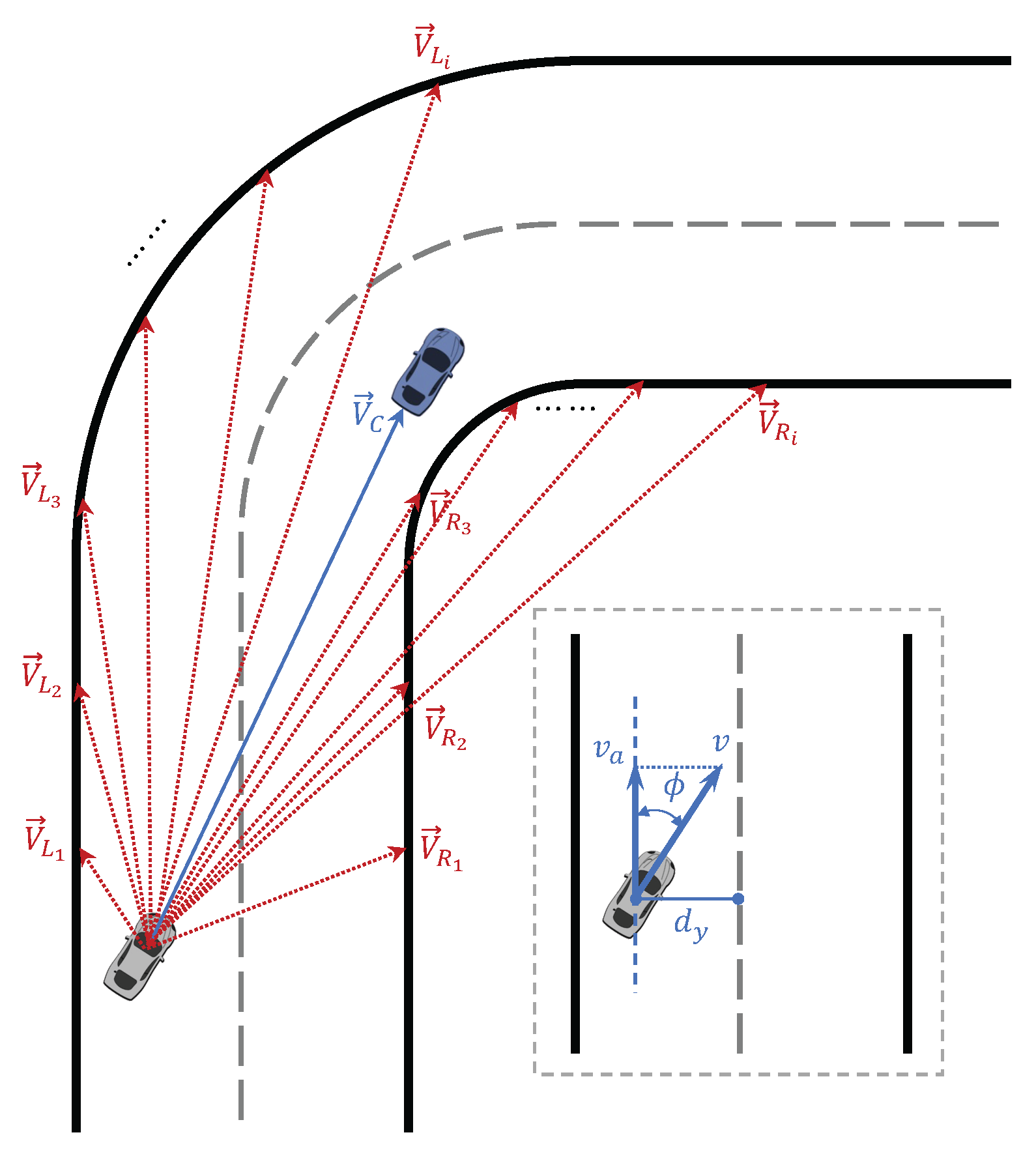
The state variables in the racing driving MDP are composed of three parts: The first set of state variables describes the vehicle’s own measured motion state, including vehicle speed
v, yaw rate
, and front wheel steering angle
. The second set of state variables describes the vehicle’s relative position on the track, as shown in
Figure 2, including the lateral distance
from the vehicle’s center to the track’s centerline, and the angle
between the vehicle’s heading and the tangent direction of the track. The third set of state variables reflects the positional information of the track edges and opponent vehicles ahead within a certain distance, composed of a series of observation vectors.
and
represent the vectors from the vehicle’s center pointing toward the left and right track edges, respectively.
represents the observation vector from the vehicle’s center to the opponent vehicles within the observable range. Specifically, taking the left edge observation vector as an example, assuming the center coordinates of the race car are
and the coordinates of the left track edge point are
, the observation vector is defined as
where
is the vehicle’s heading and
is the corresponding rotation matrix that transforms the vector from the inertial coordinate system to the vehicle’s coordinate system.
By concatenating the two sets of
edge observation vectors from both the left and right sides, we obtain the edge observation feature:
. By concatenating all the opponent vehicle observation vectors
, we form the opponent observation feature
. It is important to note that, in practice, there may be no opponent vehicles within the observable range ahead, or there may be one or more opponent vehicles. Therefore, the dimension of the vector
is uncertain, and the specific handling method is detailed in
Section 4. Finally, by combining the three sets of state variables, we obtain the state vector of the racing driving MDP, which is
3.2. Action Space
Based on the aforementioned vehicle model, the control signals consist of a combination of the normalized throttle/brake (longitudinal) control signal
and the normalized steering (lateral) control signal. Although in typical RL-based control methods, the actions are equivalent to the control signals, this is not the case in this study. Therefore, the corresponding lateral control action
and longitudinal control action
are additionally defined, and the control vector is represented as
. The specific relationship between the actions and real control signals is detailed in
Section 5.
3.3. Reward Function
The goal of racing driving is to complete the track in the shortest possible time while avoiding dangerous situations such as running off the track, skidding, and collisions between cars. Therefore, a well-designed reward function is required to correctly represent the optimization objectives, and it is defined as
where
(shown in
Figure 2) is the speed reward, which represents the projection of the vehicle’s speed along the track tangent. This term serves as an effective proxy for minimizing lap time. This approach provides more frequent reward signals during continuous operation compared to sparse lap time rewards. It also encourages both high straightaway speeds and optimal cornering speeds that maintain momentum through turns.
Except for the speed reward, all other components in the reward function are implemented as binary penalties. Each penalty term takes a value of −100 when the corresponding undesired condition is triggered and 0 otherwise. The off-track penalty
is applied when the center of the vehicle crosses the track boundary. The skidding penalty
is incurred when the vehicle’s lateral acceleration exceeds the friction limit, as defined in
Section 2. The collision penalty is triggered when the distance between the ego vehicle and an opponent vehicle falls below a safety threshold, defined as
times the vehicle length. Additionally, the slow driving penalty
and wrong-way driving penalty
are included to discourage unnecessarily slow speeds (below 20 km/h) and driving in the wrong direction, respectively.
It should be noted that although the proposed safety mechanisms can avoid skidding and car collisions, corresponding penalty terms are still included for the purpose of training baseline comparison methods.
4. State Mapping for Track Observations
Based on the description of the vehicle’s state space mentioned above, the observation of the track ahead consists of a series of vectors indicating the positions of the track edges and opponent cars. Although this method of describing the state is common in RL-based autonomous driving research, it lacks flexibility in dealing with the varying number of opponent vehicles ahead. Specifically, when there are no opponent vehicles or multiple opponent vehicles within the observable range, it becomes difficult to accurately express the current state without changing the state space dimension. Additionally, the mismatch in the state space dimension caused by incorporating the information of opponent vehicles ahead creates inconvenience in transferring driving strategies between the two common racing scenarios: with and without opponent vehicles. For example, a driving strategy trained in a scenario without opponent vehicles cannot be applied to a scenario with opponent vehicles and must be retrained, which prevents the use of techniques like transfer learning to fully utilize the results of previous training to improve training efficiency.
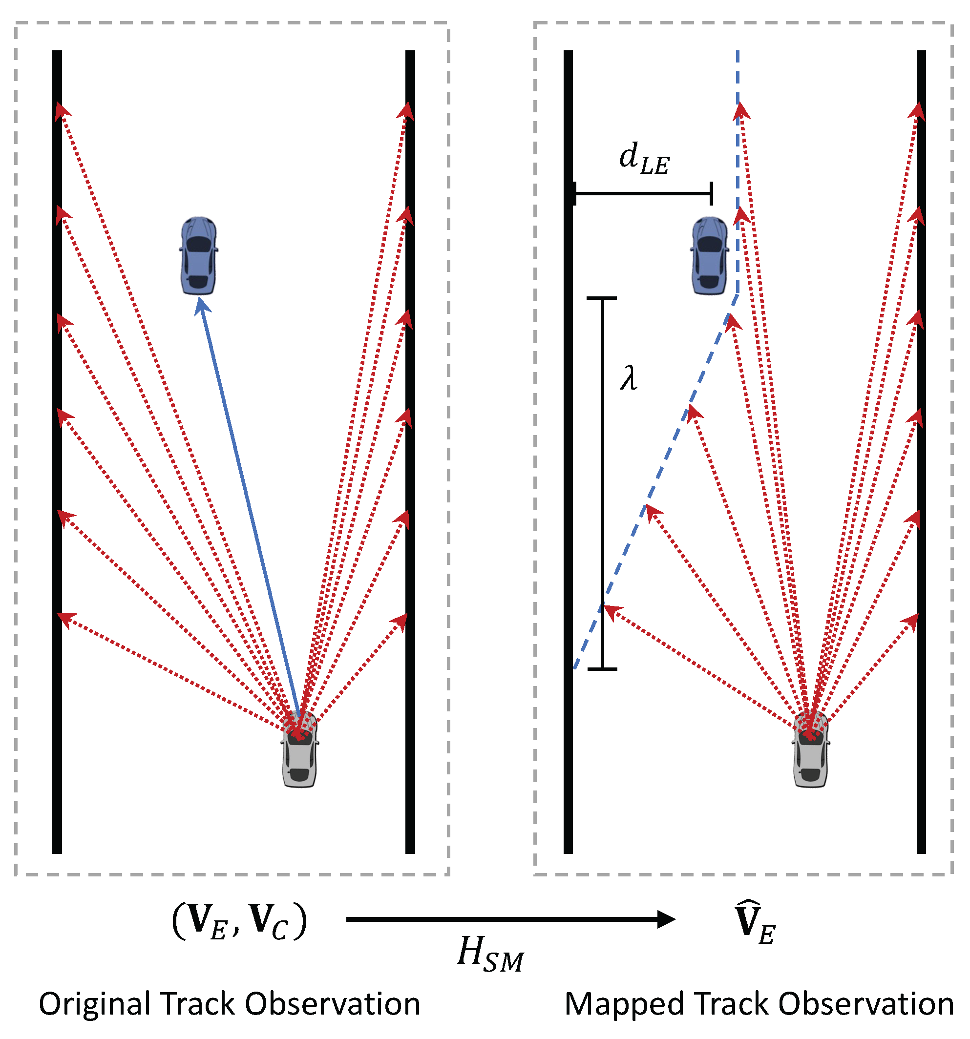
To enhance the flexibility of the racing driving strategy in the above situations, we propose the state mapping method for the track environment’s forward observation. The specific approach is shown in
Figure 3. If there are opponent vehicles within the observable range ahead, the overtaking feasible area is dynamically defined based on the positions of all observable opponent vehicles, and the original track edge observation vectors are mapped to the edge of the overtaking feasible area. To construct the feasible area, the first step is to determine whether the feasible area is on the left or right side of the opponent vehicle. The method is as follows: when the front vehicle is driving in the middle of the track, with space for safe overtaking on both sides, the side closer to the race car is chosen as the feasible area to avoid unnecessary detouring; when the front vehicle is close to one side of the track edge, the larger space on the opposite side is selected as the feasible area to ensure safety.
Next, based on the position of the front vehicle on the track and its relative position to the current car, the observation vectors of the original track edges are mapped. The focus is on calculating the positional deviation between the original track edge point and the feasible area edge point. Taking the right-side overtaking case shown in
Figure 3 as an example, let point
be located on the left edge of the track within the observable range. Let the distance along the track’s tangent direction from this point to the opponent vehicle be
, where
indicates that the track edge point is ahead of the opponent vehicle and the opposite indicates it is behind. By moving point
a distance of
to the right, perpendicular to the track’s tangent direction, it lands on the left edge of the feasible area. This point is denoted as the left feasible area edge point
, and the moved distance is defined as
where
represents the distance between the opponent vehicle and the left edge of the track,
is the lateral safety redundancy distance of the feasible area, and
is the backward extension distance of the feasible area. When
, it indicates that the entire width of the current track is a feasible area.
reflects the longitudinal safety redundancy of the overtaking feasible area. Similarly, when the right side of the opponent vehicle is considered as the feasible area, the track’s right edge point
is moved left by a distance
to obtain the right feasible area edge point
.
After obtaining the edge information of the feasible area, the original track edge observation vectors
or
can be mapped to the edge of the feasible area, forming a new track edge observation feature. This mapping relationship is expressed as
In addition, when the race car is driving in the feasible area processed by the state mapping, its observation of its relative position within the track will also change. This is equivalent to one side of the track narrowing while the car’s lateral position remains unchanged. Therefore, the state variable
, which describes the distance from the vehicle to the track centerline, is also transformed into
. After the track state space mapping processing, the state vector for the racing control MDP is represented as
The proposed state mapping method dynamically constructs overtaking feasible areas by integrating the positional information of all observable leading opponents. Compared to the original vehicle state variables, this approach maintains a consistent state dimensionality regardless of the number of opponents. Although
Figure 3 presents a single-opponent scenario for illustrative clarity, the method naturally generalizes to multi-opponent situations by uniformly processing all relevant vehicles within the observable range.
5. Action Mapping for Traction Constraint
The racing vehicle model provides traction constraints to ensure safe handling. Therefore, the control strategy of the racing car should strictly adhere to these constraints to avoid the car entering a dangerous state. This work introduces the action mapping mechanism from the our previous work on RL control problems with constraints to handle these constraints. The basic principle of the action mapping mechanism is to establish a mapping between the unconstrained virtual policy and the constrained real policy (i.e., the actual controller), which transforms the original control problem with input constraints into a general saturated constraint control problem and optimizes it using RL algorithms. This method does not alter the original RL algorithm framework but ensures that the real policy corresponding to the virtual policy satisfies the constraint conditions through a specially designed mapping function. The key to this mechanism lies in constructing a one-to-one mapping function from the virtual policy space to the real policy space. In the following, the basic theory of the action mapping mechanism and the specific method for handling traction constraints are provided.
Consider the deterministic policy case in RL, where the virtual policy for action mapping is defined as
where the continuous state space
is a compact subspace of
and
is the dimensionality of the state. Since deterministic policies for continuous action spaces are often represented by neural networks and use nonlinear activation functions like tanh to constrain the output range, the action space
is defined as
, a compact subspace of
, where
is the dimensionality of the action. The constrained true control policy is defined as
where
F is a set-valued map from
to the power set
, which describes the constraint control input space
corresponding to any
. The set-valued map
F can be described by its graph,
. The graph is a subset of the product space
, and it is the constrained state–action space for this MDP.
Let be the set of all continuous functions that map from to . Let denote the set of all continuous functions that satisfy the condition that for any given , . Specifically, is the set of all virtual polices, and is the set of all real policies.
According to the action mapping theorem (Theorem 1 in [
35]), there exists a mapping
between the virtual policy
and the real policy
, if and only if there exists a continuous mapping
such that for any given
, the mapping
is a homeomorphism between
and
. The mapping function
is defined as
. The key to the existence of the policy mapping
T is to find a mapping function
, referred to as the action mapping function. The additional conditions and theoretical proofs that guarantee the existence of this mapping are also provided in reference [
35].
Next, the action mapping mechanism is used to specifically handle the traction constraint for racing driving. As mentioned in
Section 3.2, the actions and the control signals are not equivalent, which is different from typical RL-based control approaches, and this is to align with the application of the action mapping mechanism. Specifically, the virtual policy is defined as
, where
is the virtual action vector and
represent the virtual longitudinal and lateral control actions, respectively. The actual controller is represented as
, where
and
,
are acceleration/brake and steering signals, which have been defined in
Section 2.
The constrained real policy can be obtained through the policy mapping
T, which is specifically implemented through its corresponding action mapping function:
where
is a subset of the state variables that only includes the state variables relevant to the traction constraints.
Due to the complexity of vehicle dynamics and the constraints, it is extremely difficult to provide an analytical expression for the mapping function. Therefore, we introduce a numerical approximation method from our previous work [
18] to construct the mapping function. The basic idea of this approximation method is to adjust the action vector with respect to a boundary function
. The boundary function
is the implemented version of
in this racing driving case. It indicates the safety boundary of the traction limits for the control inputs applied to the vehicle in state
. To determine the boundary function, we employ the single-track vehicle model established in
Section 2 to iteratively adjust the states of
v and
at specified numerical intervals. At each iteration, we incrementally apply larger control inputs and verify whether these inputs adhere to the traction constraints.
However, the computational complexity of the full vehicle model, particularly due to the intricate tire force calculations, makes real-time computation of the boundary function prohibitively slow. While this approach is feasible for offline simulations, real-world applications require online boundary function computation to account for dynamic variations in vehicle performance and tire conditions. To address this challenge, we maintain the original longitudinal dynamic model while adopting a simplified kinematic model for lateral motion. This simplification assumes zero slip angles for both front and rear tires, with the vehicle’s sideslip angle and yaw rate expressed as
Although this simplification may slightly reduce the accuracy of traction limit estimation, we compensate by employing a conservative maximum friction coefficient, ensuring the resulting boundary function maintains robust safety margins.
The implementation of the action mapping from
to
at state
is carried out by projecting the action vector that exceeds the boundary
onto the boundary itself, while preserving its original direction. For action vectors that lie within the boundary, no modification is made. Specifically, the action vector
is temporarily converted into polar coordinates
, where
and
represent the vector length and direction, respectively. Using the boundary function
, we can obtain the maximum allowable length in a specific direction under state
, denoted as
. Then, the implementation form of the action mapping function is represented by
where
is the operator for converting from polar coordinates to Cartesian coordinates. The details of the approach using a numerical method with the racing model to establish the mapping function are provided in reference [
18].
Through the established action mapping function, unconstrained actions are mapped to a safe control signal. This method fundamentally prevents the race car from entering uncontrollable states, while fully utilizing the maximum tire–road friction, ensuring the safety of the autonomous racing driving strategy during both the training and execution phases.
6. Safe Exploration with a Guidance Policy
In addition to the traction constraint addressed above, another primary challenge is the risk of the car running off the track, especially during the initial exploration phase. Although the action mapping mechanism for traction constraint could keep the vehicle controllable, other inappropriate actions inside the safe boundary could also cause the car to deviate from the track.
To solve this issue, we further develop an action mapping-based safe exploration guidance method. A predefined conservative track-following controller (see
Section 7 for details: Stanley lateral controller + PID speed regulator) is introduced as an initial guidance policy. Different from the conventional policy guided method for RL, in which the control actions from the guidance policy and the RL agent are directly merged, in this work, the action mapping mechanism is utilized, and it adaptively limits the exploration and updating boundary of the RL-based racing policy. The guidance policy is also iteratively updated during the training process.
Specifically, we define the guidance policy as
and the main policy as
. To guarantee a stable updating process, the exploration range and the updating step of the policy is constrained with respect to the guidance policy. The update process of the main policy is defined as
where
is the approximated state–action value function of the main policy.
is a set-valued map which maps from the state space
to the power set
, which is
where
is the constraint function for safe exploration, which limits the maximum exploration distance of the main policy with respect to the guidance policy. The map is further represented as
where
is also a set-valued map, defined as
. As mentioned before, the action space for the RL-based continuous control method is often defined as
. Hence, we define a set-valued map
to represent the unconstrained exploration range.
Similar to the action mapping framework for traction constraint, we use the graph of the set-valued map to explain the mapping approach. The graph of
is defined as
. The graph of
is defined as
.
and
represent the real exploration space and the virtual exploration space. Similarly, we can also construct a mapping function that bridges the real and virtual exploration spaces with the help of
and its graph
. According to the action mapping theory, there exists a continuous mapping
, such that for any given
, the mapping
is a homeomorphism. The mapping function is defined as
, and the implementation version of the mapping function is represented by
where
when
. Based on this mapping function
, a one-to-one correspondence is established between the real exploration space
and the virtual exploration space
through
. At this point, for any given state–action pair
in real exploration space, its corresponding exploration action
in the exploration space is
Conversely, given a state
and an exploration action
, its corresponding action in the real exploration space can be calculated by
Note that is determined exclusively by the constraint function . Consequently, modifications to the guiding policy do not influence the mapping function . This property allows us to leverage standard RL algorithms to iteratively optimize the main policy.
In addition, during training, as the main policy is optimized, it may eventually surpass the performance of the guiding policy . When this occurs, the current guidance policy can hinder further improvement of . To address this, we evaluate the main policy every episodes, using lap time as the performance metric. If the difference in lap times between the two policies, denoted as , exceeds a predefined threshold , we update the guiding policy by replacing it with the current main policy: .
7. Implementation with RL Algorithms
In this section, we detail the implementation of our proposed RL-based racing control approach, which integrates three key components: the state mapping module for track observations; the action mapping module for traction constraints; and the safe exploration guidance module. These proposed modules are compatible with most RL algorithms capable of handling continuous observation and action spaces. For illustration, we employ the classic Twin Delayed Deep Deterministic Policy Gradient (TD3) algorithm [
36] to demonstrate the implementation process.
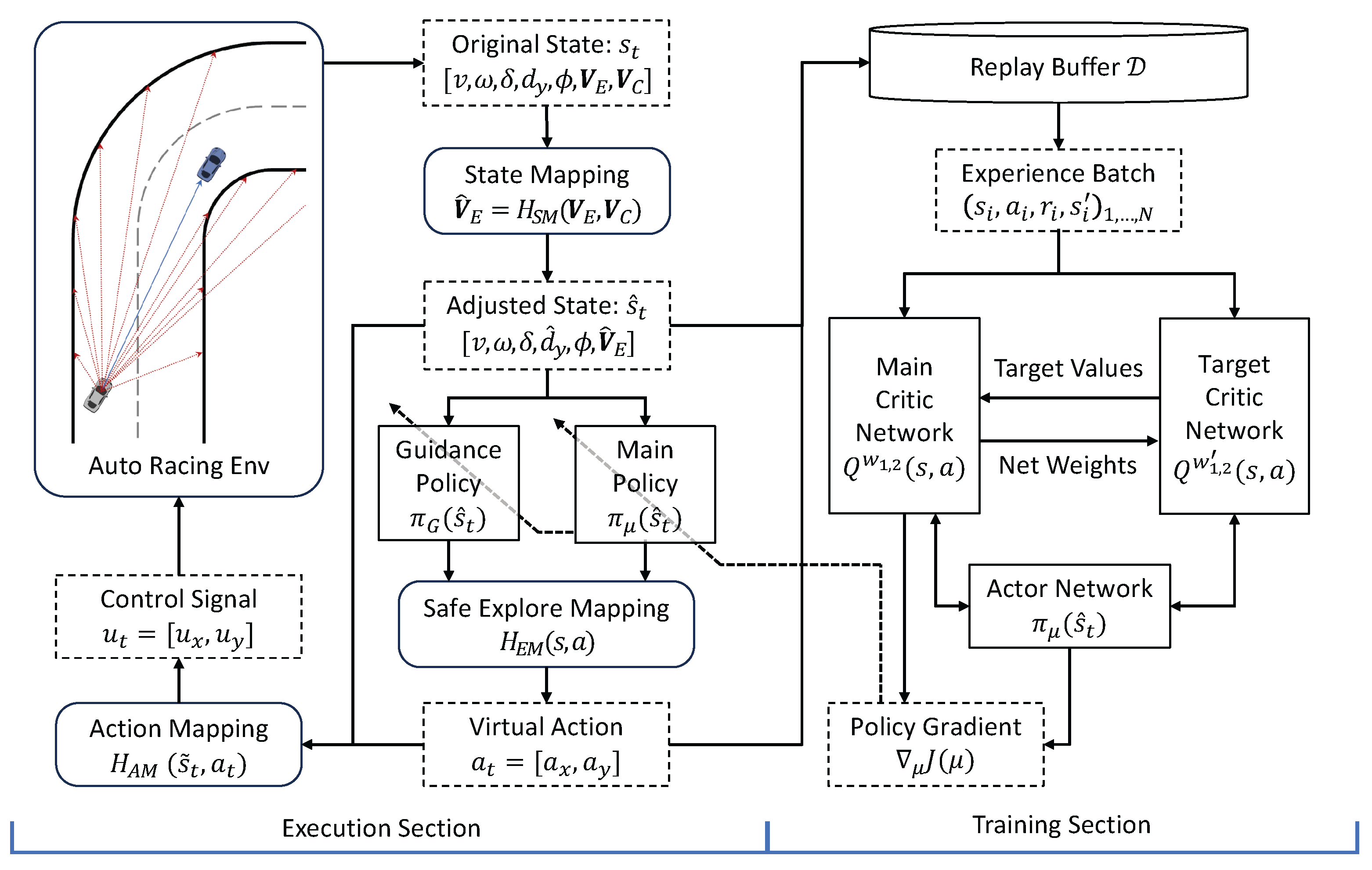
A block diagram of the proposed RL framework for autonomous racing is shown in
Figure 4. The left part of the diagram illustrates the execution section of the framework, which demonstrates the direct interaction between the autonomous driving agent and the racing environment. The state vector
is obtained from the environment observation. The edge observation feature
is defined as a set of 10 observation vectors per track edge. These vectors sample the track at increasing look-ahead distances ranging from
to
, with a uniform sampling interval of
. The original state vector
is then processed by the state mapping module
. The position information of the opponent vehicles
is integrated into the original track edge observation vector and forms
.
The processed state vector is subsequently input to the safe exploration guidance module. Within this module, an admissible control action is generated by synthesizing the guidance policy and the main policy, ensuring compliance with the predefined constraints on the exploration range. It should be noted that all state variables are normalized to either the interval or , based on their respective minimum and maximum observed values.
For the initial guidance policy, we implement a Stanley steering controller [
37] for lateral control to track the centerline. Since the Stanley control law outputs a desired steering angle, while our model accepts steering rate command rather than a direct angle input, we introduce a secondary proportional controller to compute the required steering rate. The control law is given by
where
is the steering rate gain;
is the cross-track error gain; and
is a small constant introduced to avoid division by zero. For longitudinal control, we employ a PID controller to regulate speed, maintaining a constant reference velocity through acceleration and braking commands.
It is worth noting that the initial guidance policy is primarily designed to keep the vehicle on track during early exploration. As such, suboptimal yet safe parameter tuning is sufficient. During training, this policy is gradually replaced by the learned RL policy once the latter demonstrates superior performance, as discussed in
Section 6.
Next, this action is fed into the action mapping module, where it is considered as the unconstrained virtual action. Then, by utilizing the action mapping function , the virtual action is converted to a safe control signal , which guarantees that the traction constraint is satisfied. After that, this control signal is used to control the racing car in the environment. The racing environment then returns the reward based on the predefined reward function and the next state.
The right portion of
Figure 4 depicts the RL training section of the proposed framework. We adopt the off-policy TD3 algorithm, motivated by preliminary experiments from our prior work on autonomous racing [
18], where TD3 exhibited superior training stability compared to the on-policy PPO algorithm. In particular, TD3’s twin-critic architecture effectively mitigates value overestimation while maintaining the stability required for safe operation near the limits of vehicle dynamics. Although our framework is compatible with various RL algorithms, the characteristics of TD3 make it especially well-suited for demonstrating the effectiveness of the proposed methods.
The actor and critic of the TD3 algorithm are implemented as fully connected neural networks. The actor network, denoted as with trainable parameters , serves as the main policy in the safe exploration module in the execution section. The target network of the actor network shares the same structure, and it is denoted as . Structurally, the actor network consists of two hidden layers, each comprising 256 neurons with ReLU activation. The output layer utilizes the tanh activation function to constrain actions within the range of . To address the issue of value function overestimation, the TD3 algorithm employs a twin-critic architecture. The two critic networks, represented as and with parameters and , respectively, share an identical hidden layer structure with the actor network. While the hidden layers utilize ReLU activation functions, the output layers adopt linear activation to estimate Q-values without restriction. Corresponding target networks, denoted by and , maintain the same architecture but employ slowly updated parameters to enhance learning stability. The updating rate for both target networks is set as .
The training process employs batch learning through an experience replay buffer
, which stores state transition tuples
collected during policy execution. The maximum size of the buffer is set as 1 million. Notably, the buffer records the adjusted state representation
rather than the original state. During each training iteration, a mini-batch of experience tuples
are randomly sampled from the replay buffer. The batch size
is empirically determined to balance learning stability and computational efficiency. The twin-critic networks are then independently optimized by minimizing the temporal difference (TD) error through the following loss function:
where
is the target value from the target critic networks, that is,
where
is the discount factor. To value overestimation in the target values, a clipped Gaussian noise is introduced:
, where
c denotes the clipping bound.
The actor network parameters
are updated using a sampled approximation of the policy gradient, computed through the deterministic policy gradient theorem. Utilizing the same batch of transitions and the primary critic network
, the gradient estimate is given by
The training procedure of the race driving policy with the proposed framework is formally presented in Algorithm 1, where a Gaussian noise term
is incorporated into the virtual action at each step to facilitate effective exploration. To enhance training stability, the algorithm implements a delayed policy update scheme whereby the actor network and target networks are only updated after every
iterations of critic network optimization. Additionally, the training process includes periodic policy evaluation at predetermined intervals, enabling performance monitoring and preservation of optimal policy snapshots throughout the learning process.
| Algorithm 1 Proposed RL Framework for Autonomous Race Driving |
- 1:
Initialize actor network parameters , critic network parameters - 2:
Initialize target networks parameters , , - 3:
Initialize network update parameters - 4:
Initialize replay buffer - 5:
Set initial guidance policy - 6:
Load race driving environment - 7:
for Episode = 1 to MaxEpisode do - 8:
Initialize ego car and opponent cars (if applicable) - 9:
Observe initial state - 10:
Process with state mapping: - 11:
for time step to MaxStep do - 12:
Generate exploration action: - 13:
Process with safe explore mapping: - 14:
Process with action mapping: - 15:
Execute , observe , and receive - 16:
Process with state mapping: , - 17:
Store in - 18:
Sample experiences - 19:
Update critic networks using Equation ( 28) - 20:
if t mod then - 21:
Update actor network using Equation ( 30) - 22:
Update critic and actor target networks: - 23:
end if - 24:
if car violates safety constraints then - 25:
break - 26:
end if - 27:
if Episode mod then - 28:
Run policy comparative evaluation of and - 29:
if then - 30:
Update guidance policy - 31:
end if - 32:
end if - 33:
end for - 34:
end for
|
8. Experiments and Results
This section presents a comprehensive evaluation of the proposed RL-based race driving approach within our developed racing simulation platform. In the following, we first detail the specifications of the simulation platform; then, we conduct experimental trials in two distinct racing scenarios—a time trial scenario without opponent vehicles and a competitive race scenario involving multiple opponents on the same track.
8.1. Simulation Environment
The racing driving simulation environment is built based on the single-track vehicle model established in
Section 2, and the differential equations are numerically solved using the fourth-order Runge–Kutta (RK4) method. The simulation time step is
s. The vehicle model parameters used in the simulation are derived from a pure electric mid-size sedan, and its basic physical parameters are provided in
Table 2.
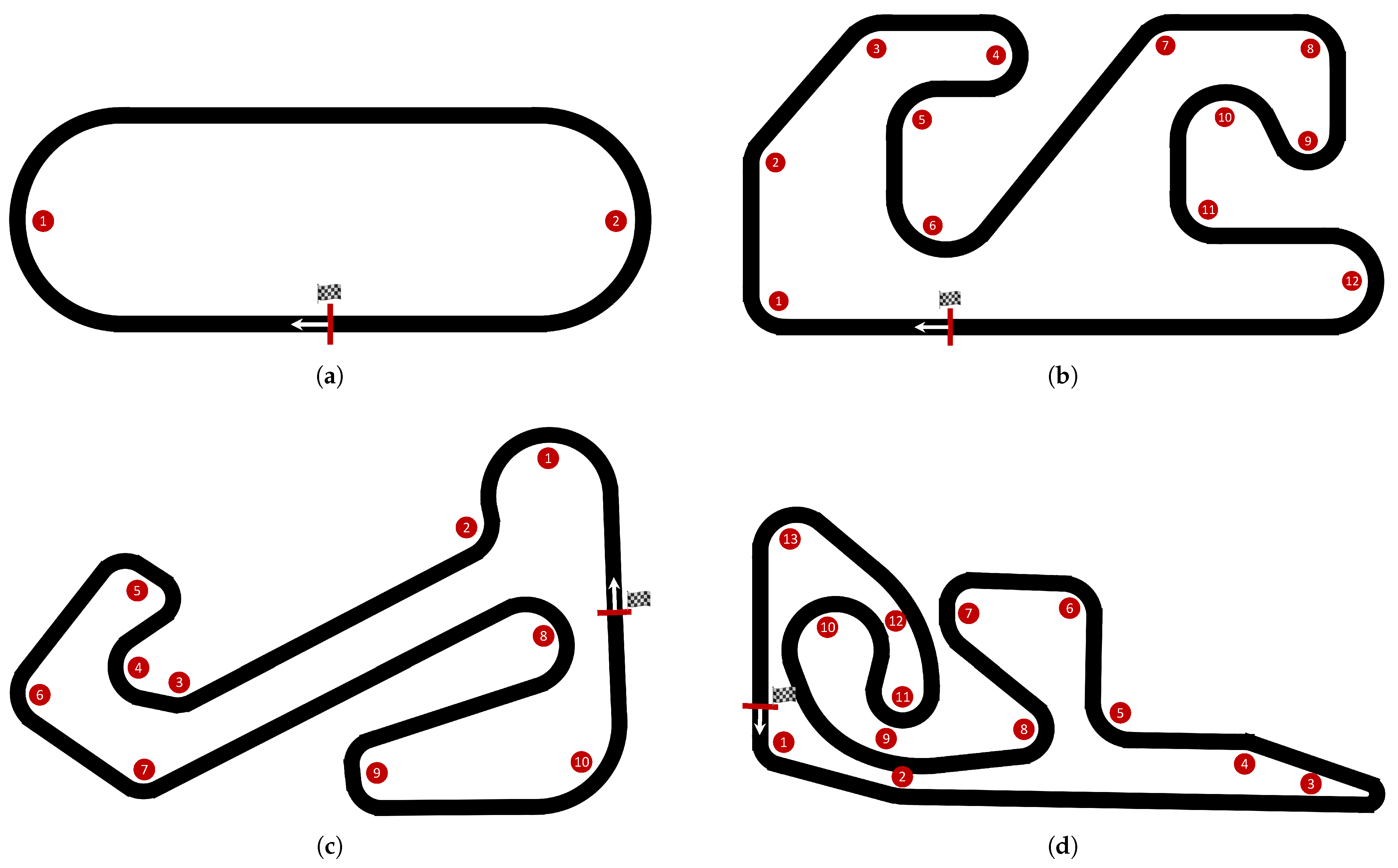
To comprehensively and thoroughly test the performance of the driving strategy, four test tracks with different styles are built in the simulation environment.
Figure 5 illustrates the track layouts, while
Table 3 summarizes their basic information. In
Figure 5, the starting line (finish line) and starting direction marked by red lines and white arrows in the respective track layout diagrams. Track A is a simple circular test track, Track B is a go-kart track with short straights and many curves, Track C is built to the same dimensions as the Ruisi Circuit located in Beijing, China, and Track D is built to the same dimensions as the Wanchi Circuit located in Nanjing, China.
The simulation experiments were conducted on a hardware platform equipped with an Intel Core i9-13900K CPU, 32 GB RAM, and an NVIDIA GeForce RTX 4090 GPU. The software environment consists of Ubuntu 20.04 LTS as the operating system, with PyTorch 1.13 serving as the deep learning framework for neural network implementation and training.
8.2. Training and Results in Time Trial
The time trial scenario as a fundamental benchmark for evaluating autonomous racing performance. Since there is no opponent car in this setup, the assessment only focuses on the action mapping module and the safe exploration guidance module, while the state mapping module is not involved. To facilitate comparative analysis, we evaluate three RL-based driving policies: (1) TD3 is the standard implementation without additional modules. (2) TD3-AM extends TD3 by incorporating the action mapping (AM) modules to address the friction constraints. (3) TD3-AMGP combines a guidance policy (GP) for safe exploration guidance.
The training of three policies follows Algorithm 1, and the unused procedures are omitted from the algorithm. For each episode the car is initialized under the following conditions: (1) initial car position: random location on straight track segments; (2) initial velocity: ; (3) other state variables: .
The assessment was conducted across four aforementioned track configurations. For each combination of policy and track, we conducted five independent training trials with distinct random seeds to ensure statistical robustness. Each trial consisted of 8000 episodes, with every episode spanning 5000 time steps (50 s). The accumulated reward values and termination reasons of each episode were recorded throughout training.
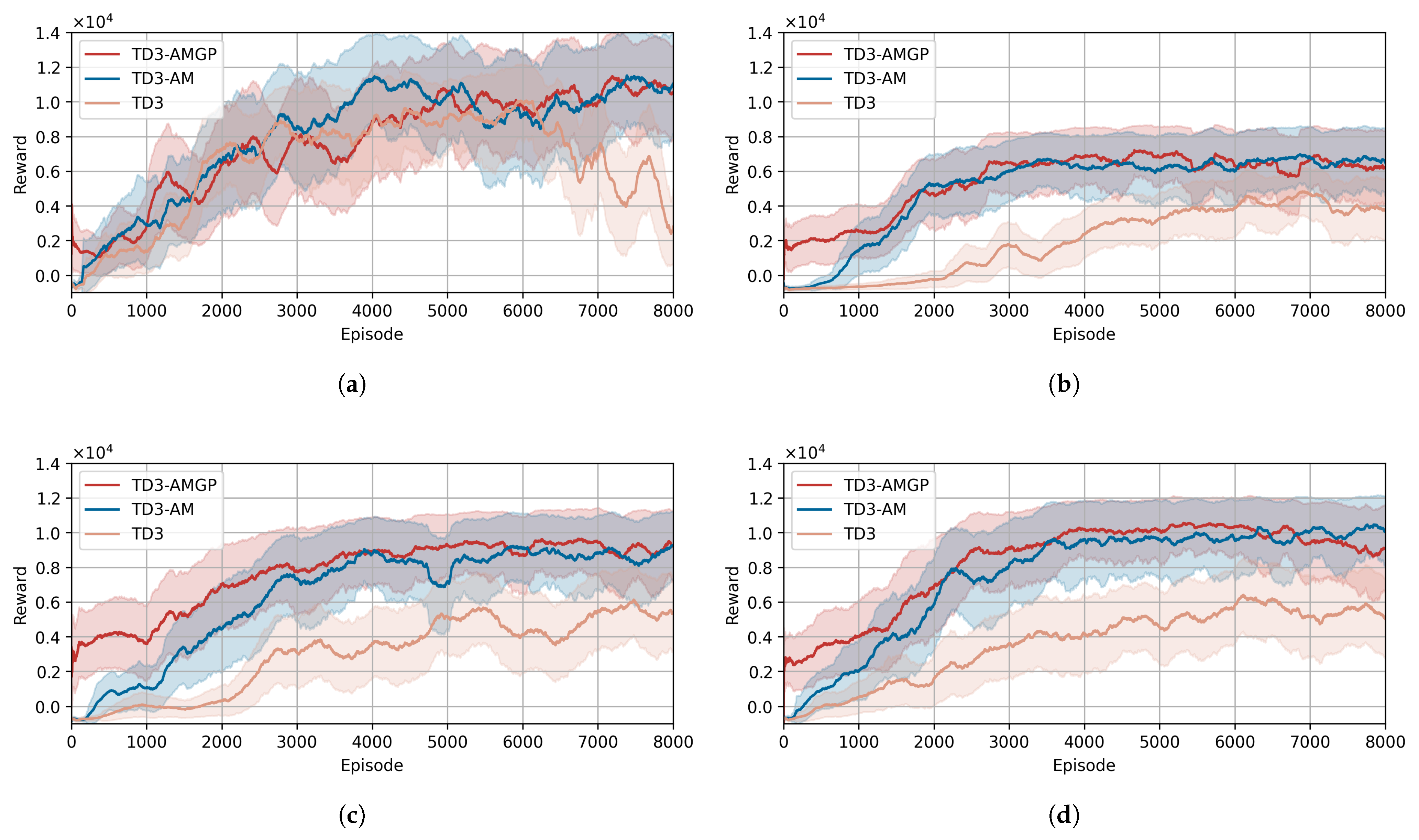
The learning progress comparison of three driving policies across four tracks is illustrated in
Figure 6. The mean rewards across seeds are plotted as solid curves, and the corresponding standard deviations are represented by shaded regions. The learning curves show that both TD3-AM and TD3-AMGP converge after around 4000 training episodes (approximately 10 million training iterations). The average training time for each of these policies is approximately 5 h. Notably, the computational overhead introduced by the safe policy guidance mechanism in TD3-AMGP is negligible. For comparison, the standard TD3 implementation completes the same number of iterations in about 4 h, due to the absence of action mapping computations.
The learning curves analysis reveals distinct performance characteristics among the three driving policies in each track. On the straightforward Track A, all policies demonstrate comparable reward progression, indicating that the basic TD3 policy can achieve competent driving in simple environments without additional modules. However, the more complex Tracks B, C, and D clearly differentiate the modules’ capabilities. The incorporation of action mapping (AM) in both TD3-AM and TD3-AMGP yields significant improvements over the baseline, with approximately 50–100% higher asymptotic rewards, by maintaining tire forces near the friction limits while preventing loss of control—enabling both faster lap times and greater stability. TD3-AMGP initially achieves higher rewards on complex tracks due to its pre-tuned guidance policy, which provides basic driving capability and prevents unsafe exploration behaviors like driving off the track. In contrast, TD3-AM requires more time to learn viable and safe driving policies through exploration. The guidance policy updating technique of TD3-AMGP effectively avoids the driving policy from becoming trapped in the initial guidance policy, enabling TD3-AMGP to eventually converge to a performance level comparable to TD3-AM. As a result, both methods eventually converge to similar performance levels, with TD3-AMGP maintaining safer exploration throughout the training process.
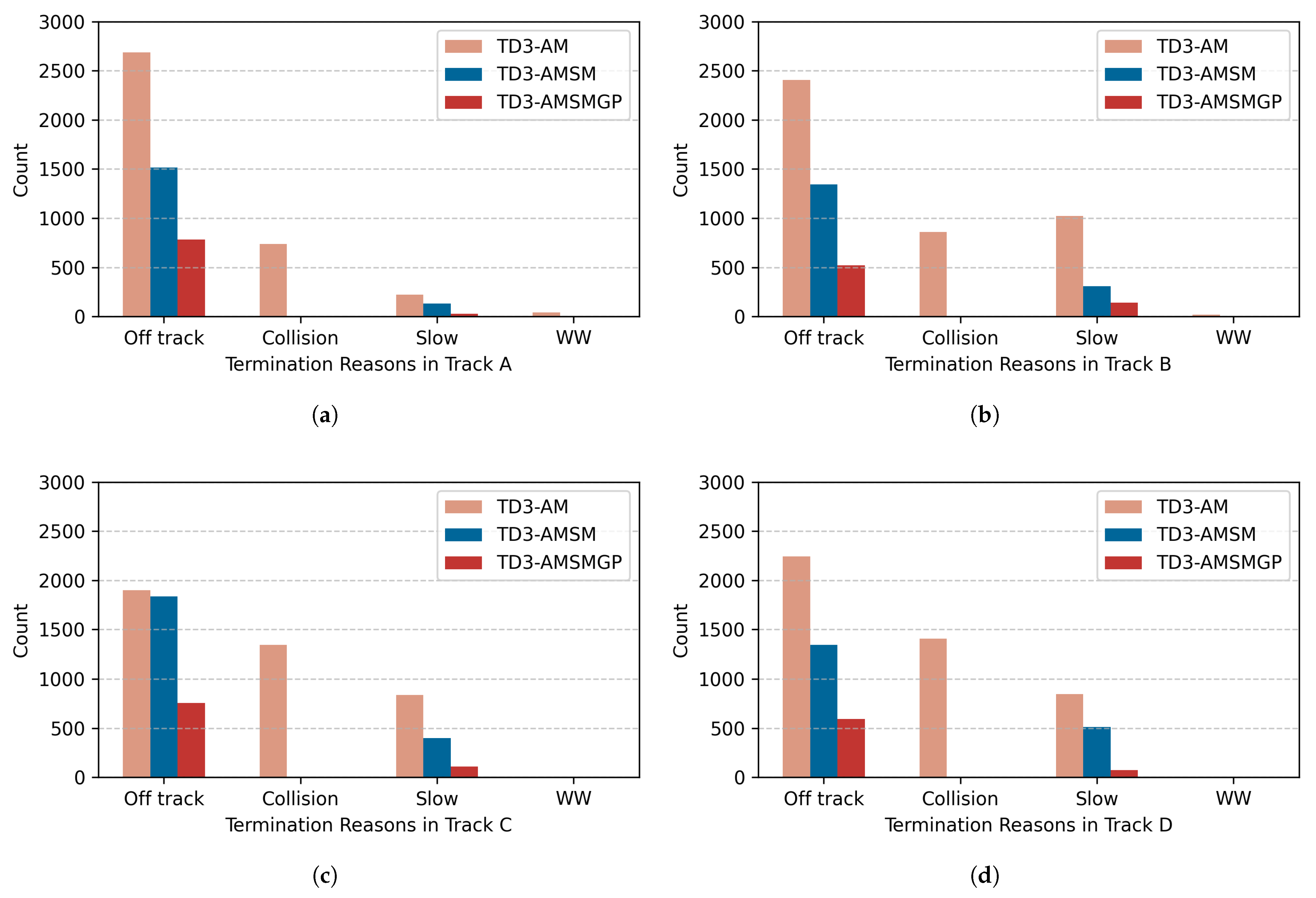
The episode termination reasons during policy training across four tracks are quantitatively analyzed. The results are visualized in
Figure 7. The termination categories correspond to the definitions in the reward function: (1) ‘off track’ represents driving off the track; (2) ‘skid’ indicates exceeding tire friction limits; (3) ‘slow’ denotes termination due to excessively low driving speed; and (4) ‘WW’ signifies driving in the wrong direction.
The statistical results show generally similar patterns of termination reasons across the three driving policies on four tracks. Specifically, the TD3-AMGP policy, due to its incorporated guidance policy, demonstrates significantly fewer off-track terminations compared to the other two methods, with approximately reduction relative to the baseline TD3 across all tracks. Furthermore, with the introduction of the action mapping module, both TD3-AM and TD3-AMGP completely avoid skid-induced terminations.
In addition, we compute the completion rate of all policies across the four tracks. The completion rate is defined as the proportion of training episodes that are successfully completed without triggering any termination conditions. The completion rates of TD3, TD3-AM, and TD3-AMGP are , , and , respectively, with TD3-AMGP achieving the highest completion rate across all four tracks.
It should be noted that although TD3-AMGP implements a guidance policy, random exploratory actions are still added during training, which may occasionally cause off-track incidents. This design is intentional—without maintaining some off-track experiences, the policy cannot effectively learn to prevent such situations. Therefore, the proposed safe exploration module can reduce but not entirely eliminate off-track occurrences during training.
To evaluate and demonstrate the driving skills of the trained driving policies, the driving policies are saved and tested in an evaluation episode for every training iterations. The lap time of a ‘flying lap’ is used to quantify driving skills. The evaluation episodes begin with the vehicle centered on the finish line with motion states , and the exploration noise is removed. If the driving policy completes at least two laps without failure, the second lap time is recorded as the ‘flying lap’ metric.
The best lap time of all saved driving policies evaluated in four tracks is summarized in
Table 4. The results demonstrate that both TD3-AM and TD3-AMGP policies, which incorporate the action mapping technique, achieve significantly faster lap times compared to the baseline. Specifically, the TD3-AMGP policy shows only marginal improvement over TD3-AM on Track B, while maintaining comparable performance on other tracks. This observation aligns with our theoretical expectation that the primary purpose of introducing the guidance policy (GP) is not to improve lap time performance but rather to improve safety during training. Consequently, as evidenced by the experimental data, TD3-AMGP achieves essentially equivalent maximum lap speeds to the TD3-AM approach while providing additional safety benefits during the learning process.
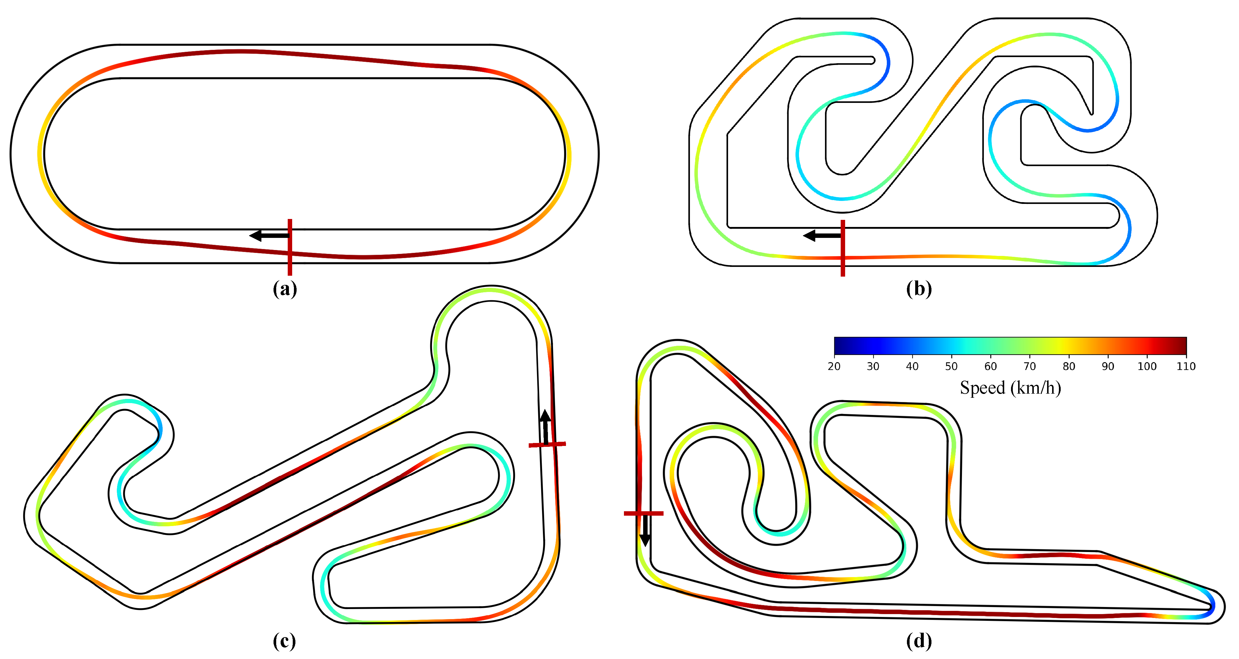
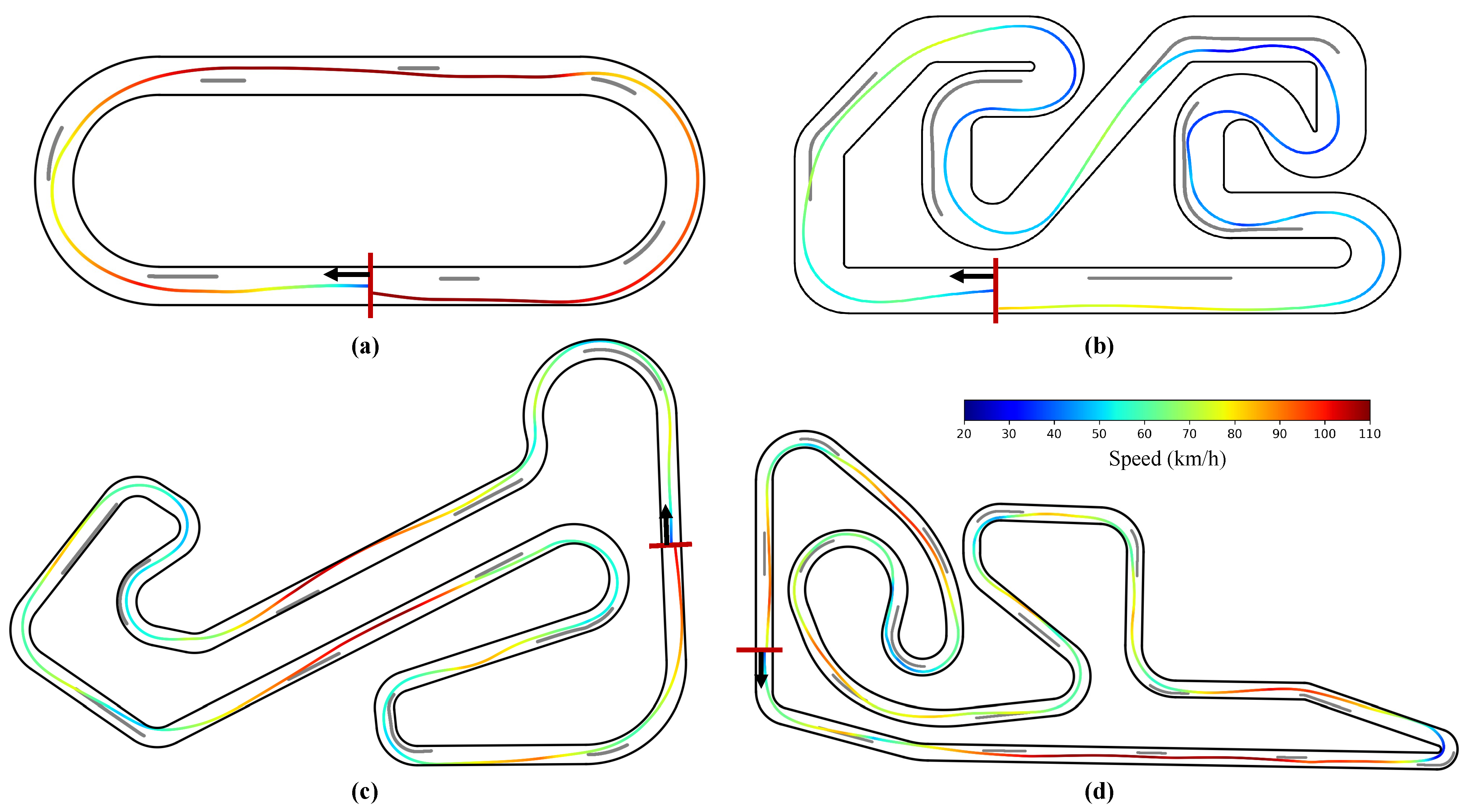
The optimal lap trajectories achieved by the TD3-AMGP policy across four test tracks are visualized in
Figure 8, where the vehicle’s instantaneous speed is color-coded using a jet colormap, with the starting line and driving direction annotated. The trajectory analysis reveals that the learned policy has mastered fundamental racing techniques, including (1) smooth racing lines following the professional ‘out-in-out’ cornering principle, (2) precise apex clipping maneuvers, and (3) optimized acceleration/deceleration strategies. Particularly impressive is the policy’s performance on the more challenging real-world tracks (Tracks C and D), where it demonstrates professional-level competence in handling complex corner sequences—maintaining ideal racing lines while executing perfect speed adjustments through consecutive turns.
8.3. Training and Results in Competitive Racing
Building upon our previous time trial experiments that evaluated autonomous racing fundamentals in single-vehicle scenarios, we now introduce dynamic opponent vehicles to assess the proposed state mapping technique. The comparative evaluation maintains consistency with prior methodology by examining three policy variants: (1) TD3-AM (baseline) is the same as the policy used in the time trial experiments. To maintain the same length of the opponent car observation vector , we only observe the nearest leading opponent car. (2) TD3-AMSM extends TD3-AM by incorporating the state mapping (SM) module to enhance the observation of opponent vehicles ahead. (3) TD3-AMSMGP integrates both SM and the guidance policy (GP) for safe exploration in competitive environments. The safe exploration guidance necessarily operates on the state-mapped representation when opponent vehicles are present. A standalone TD3-AMGP configuration would be incompatible since the guidance policy requires the transformed state variables that only the state mapping module can provide.
The training procedures for the three policies in the competitive race experiments maintain consistency with the time trial experiments, with the key distinction being the incorporation of opponent vehicles. Each opponent car is initialized with randomized parameters: a longitudinal separation of 50–150 m along the track axis, an initial velocity uniformly distributed between 20 and 60 km/h, and a variable lateral displacement from the track centerline. The opponent vehicles are controlled by predetermined controllers that maintain their initial lateral displacement while preserving the initialized velocity.
Notably, in the current setup, these opponent vehicles move at constant speeds, and their motion states remain constant over time. In addition, these opponent cars operate independently without any awareness of the ego car’s motion, serving purely as dynamic environmental obstacles to evaluate the ego vehicle’s overtaking capabilities.
Under these simplified assumptions, the feasible overtaking area is primarily determined by the opponent’s position rather than dynamic behaviors such as speed changes. Accordingly, our state mapping module focuses on spatial configuration and does not explicitly encode opponent speed or acceleration. This design allows us to address variable-dimension observation challenges while preserving policy transferability and training efficiency. This experimental setup also ensures that the assessment focuses specifically on the ego vehicle’s autonomous racing performance rather than modeling competitive interactions between vehicles. To account for the increased complexity of competitive racing compared to time trial scenarios, we have extended the training duration from 8000 to 10,000 episodes per trial to ensure sufficient policy convergence. The accumulated reward values and termination reasons of each episode were logged throughout the entire training process.
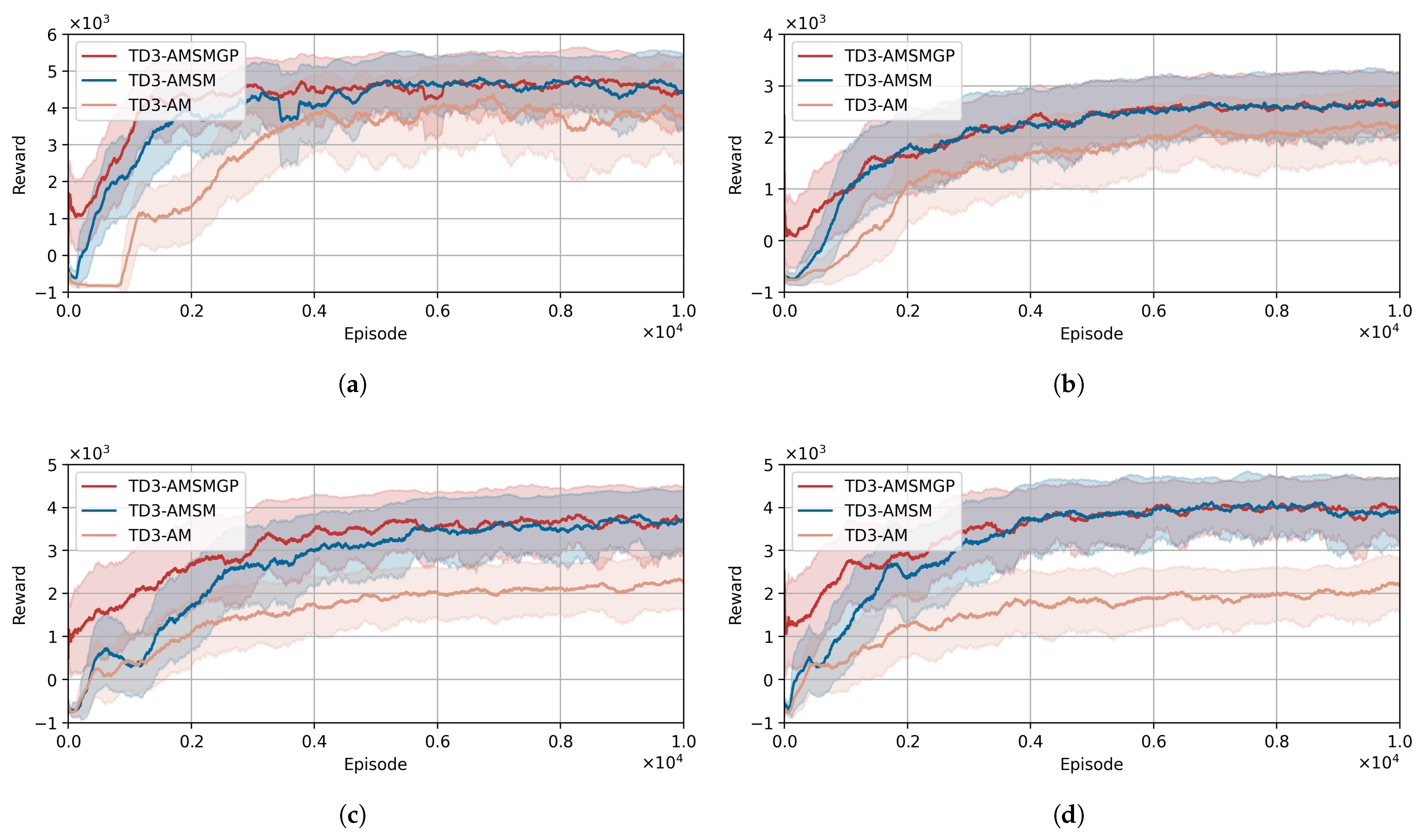
The comparative learning progress of the three driving policies across four tracks is shown in
Figure 9. The analysis of training episodes’ termination reasons is shown in
Figure 10. It is noteworthy that the termination categories are different from the time trial experiments: (1) the ‘skid’ termination category has been eliminated since the incorporation of AM in all evaluated policies effectively prevents loss-of-control scenarios caused by exceeding tire friction limits; (2) a new ‘collision’ category has been specifically introduced to episodes terminated due to contact between the ego car and opponent cars, representing a critical performance metric in competitive racing scenarios. The completion rates of TD3-AM, TD3-AMSM, and TD3-AMSMGP are
,
, and
, respectively, with TD3-AMSMGP achieving the highest completion rate.
The learning curves and termination reason statistics for the three driving policies across four tracks demonstrate consistent patterns in policy convergence and performance characteristics. All three policies exhibit stable learning progress, reaching convergence after around 6000 episodes (approximately 13 million training iterations), requiring roughly 6 h of training time. The additional computational cost introduced by state mapping and safe policy guidance modules remains minimal. Comparative analysis reveals that both the TD3-AMSM and TD3-AMSMGP methods, incorporating the SM technique, achieve significantly faster learning rates and higher cumulative rewards than the baseline TD3-AM approach on all four tracks. This performance advantage can be attributed to the substantially reduced terminations caused by collision in SM-enhanced methods, as evidenced in
Figure 10. The SM mechanism enables safer overtaking maneuvers within predefined safety margins, effectively minimizing collisions with opponent cars and consequently yielding higher rewards through improved safety performance.
Further examination of termination statistics between TD3-AMSM and TD3-AMSMGP reveals the additional benefits of GP. The TD3-AMSMGP policy demonstrates markedly fewer off-track terminations, particularly during early training phases. This reflects GP’s crucial role in guiding exploratory actions during initial training, thereby enhancing policy safety at the learning onset. This safety advantage manifests in the learning curves (
Figure 9), where TD3-AMSMGP maintains superior performance to TD3-AMSM during the first 2000 episodes, primarily due to reduced penalty accumulation from off-track incidents. The combined evidence from both learning progression and termination analysis confirms that SM and GP effectively enhance overtaking safety and efficiency in the competitive racing scenarios.
Consistent with the time trial experiments, we periodically save trained policies at 10,000-iteration intervals for subsequent evaluation. While the time trial assessment employs flying lap times to quantify basic driving skills, the competitive racing scenario necessitates a specialized evaluation framework. We therefore employ a Time Attack Overtake assessment paradigm. The Time Attack Overtake evaluation metric is designed to comprehensively assess competitive driving skills by measuring the maximum number of opponent cars overtaken within a fixed time window. The evaluation protocol initializes the ego car centered on the finish line with motion states
, and the exploration noise is removed. The opponent cars are positioned at 80m intervals along the track centerline with randomized lateral offsets and a constant initial velocity of 40 km/h. All opponent vehicles are controlled by the same predetermined controller in the training phase. Each evaluation episode is constrained to 6000 time steps (60 s). We quantitatively evaluate all saved policies by recording both the overtaking count and average velocity. The best performance metrics (number of opponents overtaken and average velocity) for each policy–track combination are presented in
Table 5. The results reveal that for the relatively simpler and wider tracks (A and B), all three driving policies demonstrate comparable performance in terms of both the number overtook and average velocity. However, in the more complex and narrower tracks (C and D), the two policies incorporating the state mapping (SM) mechanism exhibit significant performance advantages. Specifically, the SM-enhanced policies achieve approximately double the number of successful overtakes within the time window compared to the baseline approach, while simultaneously maintaining about 50% higher average velocities.
The racing trajectories of the highest-performing TD3-AMSMGP policy during Time Attack Overtake evaluations across the four tracks are illustrated in
Figure 11. The ego car’s trajectories are color-coded by instantaneous speed. The trajectories of opponent vehicles are depicted as gray lines, selectively displaying only those segments where potential interactions with the ego vehicle may occur. More precisely, for each opponent car, its trajectory visualization begins when it assumes the position of the immediate leading vehicle relative to the ego car and ceases once it has been successfully overtaken, thereby focusing the analysis on the most relevant spatial–temporal interactions during overtaking maneuvers. The trajectories demonstrate that the learned policy has successfully developed advanced overtaking capabilities while preserving the high-speed driving skills exhibited in time trials, particularly excelling in the complex, narrow configurations of Tracks C and D, where it executes both straightaway and corner overtaking maneuvers with remarkable consistency. These results clearly validate the efficacy of the SM technique in facilitating competitive driving strategies.
8.4. Discussion
The experimental results obtained from both time trial and competitive racing experiments demonstrate that the proposed RL-based driving policy can effectively learn high-performance driving strategies in environments with or without opponent vehicles. Through systematic training, the policy acquires professional-level cornering and overtaking skills while maintaining superior performance across diverse track configurations. The comparative studies of different policy configurations—incorporating AM, GP, and SM modules with the TD3 framework—respectively, validate (1) the AM module’s efficacy in handling tire–road friction constraints, (2) the GP module’s capability to enhance training safety during initial learning phases, and (3) the SM module’s effectiveness in improving competitive overtaking performance. Together, these components form a comprehensive autonomous racing solution that addresses the multifaceted challenges of high-speed vehicle control.
Despite the strong performance demonstrated, several limitations remain that could impact the real-world applicability and robustness of the proposed framework:
The inherent trial-and-error nature of RL algorithm introduces safety concerns. Although a safe guidance policy is used to constrain exploration during training, exploratory noise remains necessary for learning. This can occasionally lead to off-track incidents, and the simulation environment cannot fully replicate real-world vehicle dynamics and environmental variability. Consequently, the safety guarantees achieved in simulation may not directly carry over to real-world deployments.
The behavior of opponent vehicles is relatively simple. Currently, opponents follow predetermined trajectories and do not respond to the ego vehicle’s actions. In real racing scenarios, opponents often exhibit adaptive behaviors, such as defending lines and blocking overtakes, which are crucial to competitive driving. This limitation reduces the policy’s ability to learn complex interaction skills.
The state mapping mechanism currently uses static parameters to define the overtaking feasibility areas. These parameters do not adapt based on the motion of surrounding vehicles. As a result, the policy may generate overly conservative or aggressive decisions during overtaking.
9. Conclusions and Future Work
This paper presented an integrated RL framework for autonomous race driving that combines state mapping, action mapping, and safe exploration guidance to achieve high-performance racing while ensuring safety. Experimental results across four test tracks demonstrate substantial improvements over baseline methods in both time trial and competitive racing scenarios. In time trial scenarios, the RL-based driving policy with action mapping and safe exploration guidance (TD3-AMGP) achieved a 12–26% reduction in lap time compared to the standard TD3 policy, while the completion rate improved significantly from 33.1% (TD3) to 78.7% (TD3-AMGP), indicating enhanced training safety. In competitive racing scenarios, the proposed TD3-AMSMGP policy doubled the number of successful overtakes on complex tracks (Tracks C and D) compared to TD3-AM, while sustaining a 46–51% higher average speed. Across both scenarios, the inclusion of state mapping and the safe guidance policy effectively reduced off-track and collision-induced terminations by a large margin. These results confirm the proposed framework’s effectiveness in achieving professional-level autonomous racing performance with a strong emphasis on safety and reliability.
Future work will focus on addressing the identified limitations through the following directions: (1) enhancing safety in real-world deployment by integrating RL policies with conventional control methods, such as model predictive control and control barrier functions, complemented by real-time risk assessment techniques; (2) improving competitive driving skills by incorporating interactive opponent behaviors via adversarial multi-agent RL or imitation learning, enabling the ego vehicle to acquire adaptive and tactical driving strategies; (3) developing dynamic state mapping mechanisms that adjust the parameters for generating overtaking feasible area in real time based on the opponent motion information; and (4) exploring sim-to-real transfer techniques such as domain randomization and adaptive simulation calibration to improve the robustness and deployability of learned policies in real-world racing environments.


