1. Introduction
With the advancement of robotics technology, robotic manipulators are increasingly used in various fields of production and manufacturing due to their high flexibility and low cost. Motion planning is one of the essential technologies in robotic applications and a key research focus. Research on robot motion planning mainly involves two stages: path planning and trajectory planning. A robot path refers to the geometric description of the robot’s posture and position in the workspace, typically defined by the pose at given path points or specific path lengths. A robot trajectory is the time parameterization of the path, generally expressed as the robot’s pose as a function of time.
Robot trajectory planning generally encompasses two primary task types: point-to-point (PTP) tasks and path-following (PF) tasks. In PTP trajectory planning, only the initial and target poses of the robot are specified. As a result, planning is typically conducted in the joint space, with a focus on task feasibility and execution efficiency. This type of planning is commonly employed in simple robotic operations, such as material handling. In contrast, the PF trajectory planning requires the robot to move along a predefined path. In addition to feasibility and efficiency, it places greater emphasis on the quality of motion execution, including path accuracy and motion smoothness. Such planning is widely adopted in precision-critical applications, such as robotic milling, welding, and polishing. Consequently, compared with PTP tasks, PF trajectory planning imposes more stringent requirements on motion quality and involves more complex constraints.
For path-following trajectory planning tasks, researchers have proposed several methods. Some have introduced curve-based feedrate scheduling (CBFS) methods, which are well developed in CNC machining, into robotic trajectory planning, such as S-curve-based and polynomial-based feedrate scheduling methods [
1,
2,
3,
4]. Xu et al. [
5] proposed a dynamic window-based look-ahead feedrate scheduling method using an S-curve profile, achieving feedrate planning for a six-degree-of-freedom robot under kinematic constraints. Li et al. [
6] generated an initial feedrate profile using B-splines and then adjusted it in regions that violated kinematic constraints to produce a feasible trajectory. These CBFS methods offer clearly defined constraints and high computational efficiency and are widely applied to online feedrate scheduling in both CNC and robotic machining. However, CBFS can not optimize the trajectory and therefore cannot fully exploit the robot motion capabilities. Other researchers have used dynamic programming (DP) to address trajectory planning. Kaserer et al. [
7] formulated an optimization problem incorporating jerk constraints and motor models, and proposed an improved DP algorithm with phase-plane interpolation to ensure derivative continuity and generate smooth executable trajectories. Wu et al. [
8] transformed the energy-optimal trajectory planning problem into a multi-stage decision problem and solved it using DP. Similarly, Ding et al. [
9] applied DP in the discrete domain to search for approximately optimal trajectories under kinematic and dynamic constraints. However, due to the exhaustive search nature of dynamic programming in the discrete domain, these methods often suffer from low planning efficiency. In addition, some studies have adopted numerical integration methods [
10,
11,
12,
13] to iteratively generate time-optimal trajectory. To achieve trajectory planning with various performance objectives, researchers have increasingly formulated the problem as an optimization model and applied corresponding solution methods, targeting objectives such as time optimality [
14], energy efficiency [
15], jerk minimization [
16], or multi-objective optimization [
17,
18].
In optimization-based trajectory planning, the problem is typically formulated as an infinite-dimensional optimization model, which is then discretized through path sampling into a finite-dimensional form. Despite this transformation, the resulting problem remains nonlinear and high-dimensional due to the complexity of robotic kinematics and dynamics. To address these challenges, some researchers have reformulated the trajectory planning problem as a convex optimization model to leverage its computational advantages. Debrouwere et al. [
19] and Lin et al. [
20] demonstrated that joint torque rate constraints disrupt problem convexity. By expressing these nonconvex constraints as differences in convex functions, they reformulated the problem with convex–concave constraints and solved it using sequential convex programming. Ma et al. [
21] employed convex optimization to compute forward and backward maximum velocity curves (MVCs), solving a finite number of convex subproblems at each path point to obtain time-optimal trajectories. Zhang et al. [
22] applied sequential quadratic programming (SQP) to generate smooth and time-optimal manipulator trajectories. Liu et al. [
23] and Nagy et al. [
24] linearized nonlinear constraints and adopted linear programming (LP) to minimize the sum of velocities at sampled points, achieving time-optimal solutions. Wu et al. [
25] and Shen et al. [
26] formulated the time-optimal trajectory planning problem in the standard form of second-order cone programming (SOCP) and subsequently solved it using SOCP methods. Compared with other optimization-based approaches, convex optimization offers simpler formulations and faster computation. Moreover, the availability of commercial convex solvers further reduces the complexity and computational cost of solving convexified trajectory planning problems.
One of the key challenges in robot trajectory planning is to obtain an optimal solution under complex and diverse constraints. These constraints mainly include joint-space and Cartesian-space constraints. Joint-space constraints refer to the kinematic and dynamic limits of joints, while Cartesian-space constraints pertain to the kinematic limitations of the end-effector within the workspace. Some trajectory planning methods for path-following tasks consider only joint-space constraints [
7,
21,
27,
28,
29,
30]. However, for path-following tasks, especially in robotic machining applications, the quality of task execution is directly affected by the motion of the end-effector, making it necessary to impose additional kinematic constraints on the end-effector motion [
5,
31,
32]. In some studies, only joint velocity, acceleration, and torque limits are considered, while jerk constraints are omitted [
19,
29,
33,
34]. Several researchers have demonstrated that incorporating joint jerk constraints in trajectory planning can effectively suppress vibration during robot operation and improve trajectory smoothness [
28,
30,
32]. Furthermore, most of the above methods operate in the discrete domain, where pseudo-acceleration is often assumed constant and the square of pseudo-velocity is modeled as a linear function. This simplification causes joint torques at the boundaries of discrete intervals to become nonlinear and discontinuous, leading to severe vibration and jerks in the resulting trajectory [
25,
35]. Therefore, ensuring the continuity of joint motion is also essential in trajectory planning.
This paper proposes a time-jerk optimal trajectory planning (TJOTP) method for robots, considering compound constraints and joint motion continuity. To enhance the completeness of constraint modeling, an optimization framework is established for path-following tasks under compound constraints, incorporating both joint jerk limits and Cartesian-space kinematic constraints of the end-effector (EE). To reduce jerk and improve motion smoothness, sufficient conditions for achieving the C3 continuity of joint trajectories are analyzed, and the trajectory optimization problem is reformulated using cubic spline interpolation. A direct transcription method is adopted to construct a finite-dimensional optimization problem. To further suppress joint jerk and enhance motion smoothness, a jerk evaluation term is introduced into the objective function, yielding a time and jerk co-optimization model. To improve the planning efficiency, constraint tightening and convex relaxation techniques are applied to linearize the model, enabling its solution via SOCP. Experimental results validate the effectiveness of the proposed method in optimizing both execution time and joint jerk under compound constraints.
The remainder of the manuscript is structured as follows. In
Section 2, the time-optimal trajectory planning (TOTP) problem under compound constraints is modeled. The TOTP model is first formulated, followed by an analysis of the C
3 continuity requirement for joint motion. To fulfill this requirement, segmented cubic splines are employed to reconstruct the TOTP model. The infinite-dimensional problem in the continuous domain is then converted into a finite-dimensional problem in the discrete domain through direct transcription. In
Section 3, the TOTP problem with nonlinear and non-convex jerk constraints is decomposed into two second-order cone programming problems. A jerk evaluation term is introduced into the objective function, leading to the formulation and solution of a time-and-jerk optimal trajectory planning problem. In
Section 4, the effectiveness of the proposed method is demonstrated through experimental validation.
Section 5 provides the conclusions.
3. Problem-Solving via SOCP
In the optimization problem described by Equation (33), the objective function is convex, and all constraints, except for the jerk constraints, are also convex. Therefore, the convex optimization approach is employed to solve the trajectory planning problem. Given the non-convex nature of the jerk constraints, a two-stage SOCP method is proposed in this section. The problem in Equation (33) is decomposed into two convex subproblems, each solved using SOCP. In the first stage, a trajectory planning problem without jerk constraints (TOTP-2C) is solved. In the second stage, the optimal solution obtained from the first stage is used to convexify the jerk constraints, and a jerk evaluation term is incorporated into the objective function. Based on this, a time-and-jerk optimal trajectory planning model (TJOTP-3C) that considers jerk constraints is formulated and solved.
3.1. Modeling and Solution of the TOTP-2C Problem
When jerk constraints are not considered, the optimization model in Equation (33) becomes a convex problem. Due to the presence of square root and fractional terms in the objective function, second-order cone programming (SOCP) is adopted for efficient solution. Compared with linear programming (LP) and nonlinear programming (NLP), SOCP offers greater modeling capability and is especially suitable for handling optimization problems that involve norm terms, fractional terms, or square root terms. A standard SOCP formulation consists of a linear objective function and second-order cone constraints, and may also include linear equality and inequality constraints, enabling efficient solutions for complex but convex optimization models.
Although the objective function in Equation (33) is convex, it is nonlinear. To improve computational efficiency, auxiliary variables
and
are introduced to linearize the original function, resulting in a linear objective function expressed as
The velocity constraints in joint space and Cartesian space are also nonlinear but convex. Their linearized forms are given as
At this point, the SOCP model for the TOTP-2C problem has been fully formulated and can be expressed as
Equation (37) conforms to the standard SOCP form after linearization. Due to the structured formulation of SOCP, many mature convex optimization tools are available for solving large-scale SOCP problems efficiently. A wide range of commercial and open-source solvers provide native support for SOCP, including MOSEK, GUROBI, SCS, ECOS, and SDPT3. Among these, MOSEK demonstrates strong numerical stability and fast convergence, making it particularly suitable for trajectory optimization problems involving a large number of variables and complex constraint structures. In this study, MOSEK is selected as the solver for SOCP problems.
3.2. Modeling and Solution of the TJOTP-3C Problem
This section extends the TOTP-2C model by introducing jerk constraints to reduce impact during robot motion. In addition, to prevent potential issues caused by improper jerk bounds, the jerk evaluation term is added to the objective function. On this basis, a time and jerk optimal trajectory planning (TJOTP-3C) problem is formulated. This approach aims to suppress jerk effects and improve the smoothness of robot motion.
Based on Equation (33), the jerk constraint for the
k-th joint of a manipulator with
N joints can be reformulated as
The nonlinearity and non-convexity of the above constraint undermine the convexity of the trajectory planning problem. To enable the use of the SOCP method, the jerk constraint needs to be transformed into the linear convex form.
The TOTP-3C problem is formulated by adding jerk constraints to the TOTP-2C model. Therefore, the solution
that satisfies the constraints of the TOTP-3C also satisfies those of the TOTP-2C problem. Let
denote the optimal solution of the TOTP-2C problem; we have
[
23]. This property can be used to linearize the original joint jerk constraint as follows:
If
, then for the
k-th joint of the robot, there exists
In this case, the joint jerk constraint can be tightened as
- 2.
If
, there exists
In this case, the joint jerk constraint can be tightened as
By combining Equations (40) and (42), the linearized form of the original joint jerk constraint is obtained as
where
is known. The resulting constraint is linear and convex, and is directly compatible with the standard SOCP form, allowing for efficient computation. By applying the same constraint-tightening method, the linearized form of the EE jerk constraint is obtained as
It is important to note that due to the constraint tightening used to linearize the original joint and EE jerk constraints, the resulting solution is approximately time-optimal rather than strictly optimal. As a result, the theoretical optimality of time minimization is partially compromised. However, considering the trade-off between computational efficiency and execution performance, this approach offers a practical and effective solution for trajectory planning in real-world robotic applications.
In addition to enforcing jerk constraints, this work incorporates a joint jerk evaluation metric into the objective function, together with execution time, to formulate a weighted multi-objective optimization model. This approach enables a more balanced trade-off between execution efficiency and trajectory smoothness. By explicitly penalizing jerk in the objective, the resulting trajectory not only satisfies the jerk constraints but also actively suppresses joint jerk, leading to improved motion quality and overall planning performance.
By introducing a joint jerk evaluation metric into the objective function in a weighted form, the time-jerk evaluation function is constructed as
where
represents the jerk index at the
j-th discrete point, calculated as the sum of absolute joint jerk values, that is
It can be observed that
is a non-convex function. To enable convex reformulation, the optimal solution
of the TOTP-2C is introduced, and
is transformed into
Although Equation (47) does not directly represent the joint jerk, the preceding analysis suggests that minimizing
can help suppress the actual joint jerk, given that
. Moreover, since Equation (47) involves absolute value operations, auxiliary variables
are introduced to linearize the objective function. The resulting linear objective function is expressed as
Equation (48) involves both the time evaluation term and jerk evaluation term, which differ in physical units and numerical scales. To eliminate the impact of these differences on the optimization process, normalization is applied. In addition, although the jerk evaluation term is included, the primary objective remains the minimization of execution time. To prevent the jerk evaluation term from disproportionately influencing the optimization, a weighting factor
is introduced to balance its contribution. This design provides flexibility to accommodate varying requirements across different robotic applications. The final objective function of the TJOTP-3C problem is designed as
where
and
denote the time evaluation term and the jerk evaluation term, respectively, computed from the optimal solution of the TOTP-2C problem. By integrating the linear jerk constraints and the proposed objective function into the TOTP-2C framework, the resulting optimization model for TJOTP-3C is formulated as
Equation (50) also conforms to the standard form of SOCP, and can therefore be solved using MOSEK.
4. Experimental Validation
This section validates the effectiveness of the proposed trajectory planning method using the serial 6R robot AN5, as illustrated in
Figure 2. The DH (Denavit–Hartenberg) parameters of the AN5 robot are summarized in
Table 1. The algorithm was implemented on a personal laptop equipped with an Intel Core i5-8300H CPU (2.30 GHz) and 8 GB of RAM. Three sets of experiments were conducted to verify the following aspects: (a) the effectiveness of the proposed C
3 continuity constraints, (b) the effectiveness of the time-jerk optimization, and (c) the comparative performance of the proposed TJOTP-3C method.
It is worth noting that the paths used in the validation experiments were generated using a custom-developed linear path local smoothing method with C
3 continuity. Both the position and posture paths are C
3 continuous with respect to the path length. This satisfies the first sufficient condition for achieving C
3 continuity in the joint trajectory, namely that the given path itself must be C
3 continuous. The paths used in this study are all defined in the Cartesian space. As shown in
Figure 3, the position and posture of the robot EE are represented by the position
of the EE coordinate system {
TCP} in the robot base coordinate system {
B}, and the ZYX Euler angles
. The homogeneous transformation matrix from {
TCP} to the robot base coordinate system {
B} can be calculated as
where
represents the position vector of the EE with respect to the base coordinate system, and
represents the rotation matrix of the EE with respect to the base coordinate system, which determines the EE posture. It can be calculated from the ZYX Euler angles as
where
,
and
denote the rotation matrices about the fixed x-, y-, and z-axes of the coordinate system, respectively. According to the inverse kinematics model of the robot, the joint angles can be determined from the Cartesian-space path, i.e.,
, where
represents the inverse kinematics function of the robot.
4.1. Validation of Continuity Constraint Effectiveness
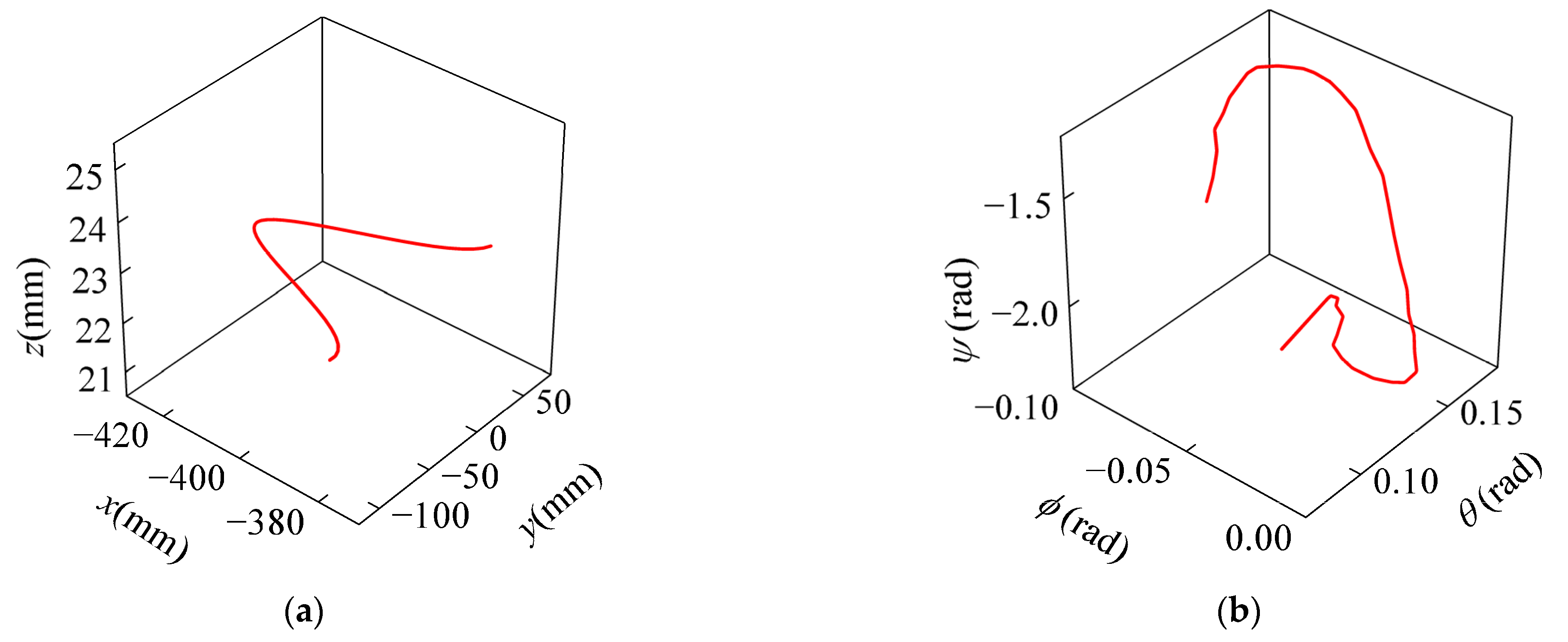
To validate the effectiveness of the continuity constraints, the butterfly-shaped EE path shown in
Figure 4 is used as a test case. Based on the Cartesian path shown in
Figure 4, the corresponding joint path
can obtained through the robot’s inverse kinematics. By differentiating the joint path, the first-, second-, and third-order derivatives with respect to the path parameter s, namely
,
and
, are computed, as illustrated in
Figure 5. It can be observed that the values of
,
and
vary with the path parameter s. According to Equation (3), given the joint-space kinematic limits, if
,
and
are large at a certain point along the path, the velocity, acceleration, and jerk in Cartesian space must be reduced to ensure that the joint motion remains within the allowable limits.
The trajectory planning results are compared under two conditions: with continuity constraints (TOTP-2C) and without continuity constraints (TOTP-2). The time-optimal trajectory planning model with continuity constraints is provided in Equation (37). In the model without continuity constraints, pseudo-acceleration is typically estimated from the pseudo-velocity squared using a finite difference formula [
23,
24], that is
When Equation (53) is used, the pseudo-velocity becomes a piecewise linear function and the pseudo-acceleration becomes piecewise constant [
25]. In this case, the pseudo-velocity is only C0 continuous, and the pseudo-acceleration is discontinuous. Such conditions can lead to sudden jumps in both acceleration and jerk in the resulting trajectory.
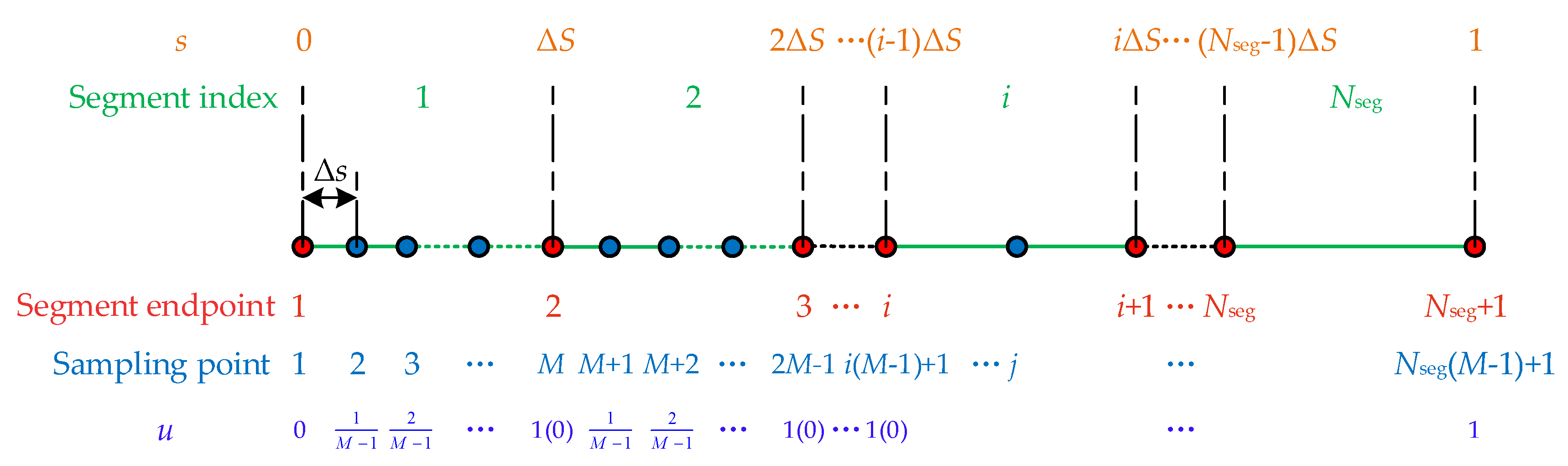
For the omega-shaped path, the upper limits of joint velocity and acceleration are set to and , respectively. The commanded feedrate of the EE is F = 10 mm/s, the maximum allowable acceleration is Amax = 100 mm/s2, and the chord error constraint is set to . In the TOTP-2C method, the path is divided into 150 cubic spline segments, with 10 discrete points sampled per segment, resulting in a total of 1351 discrete points along the entire path. The number of discrete points in the TOTP-2 method is also set to 1351 to ensure a fair comparison.
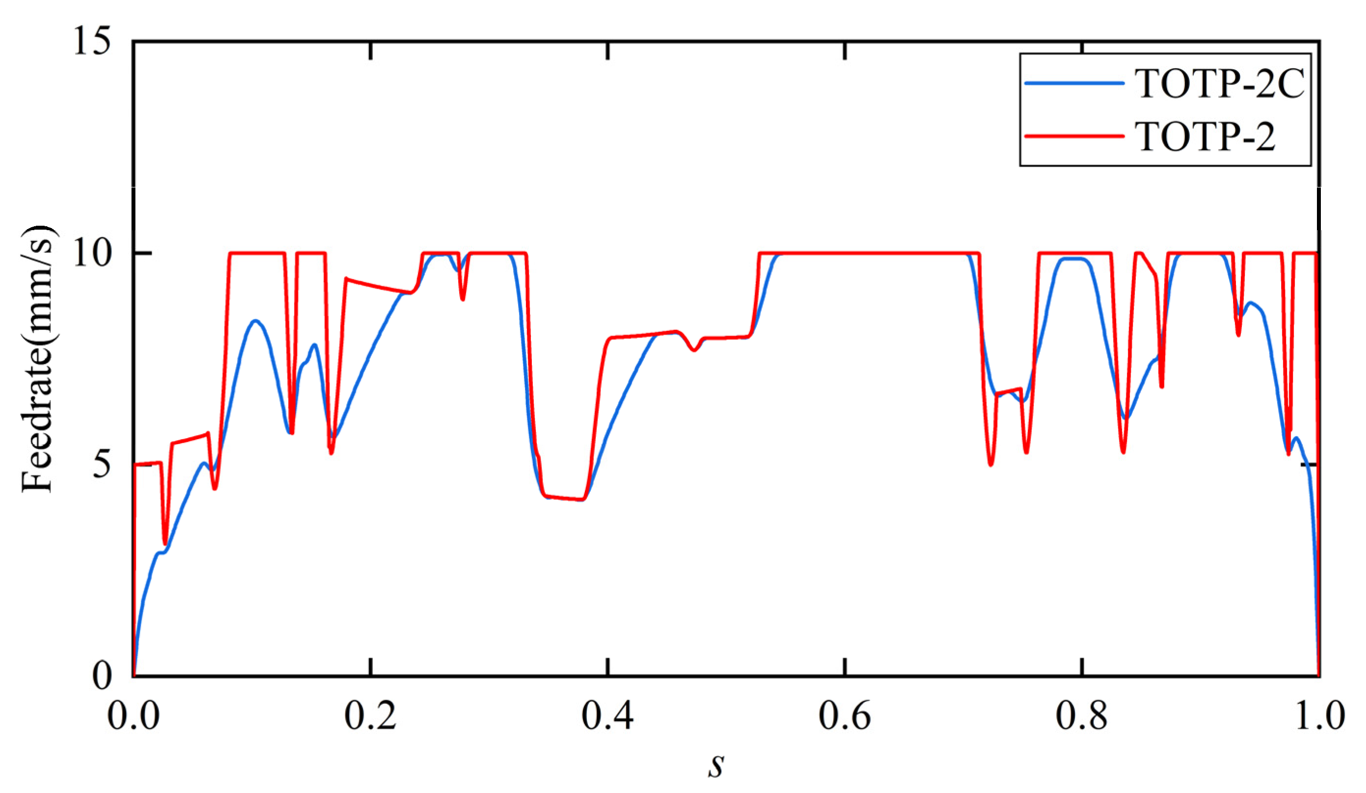
The feedrate profiles generated by the TOTP-2 and TOTP-2C methods are shown in
Figure 6. As observed, both methods produce feedrate curves with similar overall trends. However, in certain regions, the feedrate generated by TOTP-2 is slightly higher than that of TOTP-2C. The total execution time of the trajectory generated by the TOTP-2C method is 22.69 s, compared to 24.36 s for the TOTP-2 method. Although the inclusion of continuity constraints slightly increases the execution time, the feedrate curve produced by TOTP-2C is noticeably smoother. This improved smoothness contributes to enhanced trajectory quality and reduced vibration during robot motion.
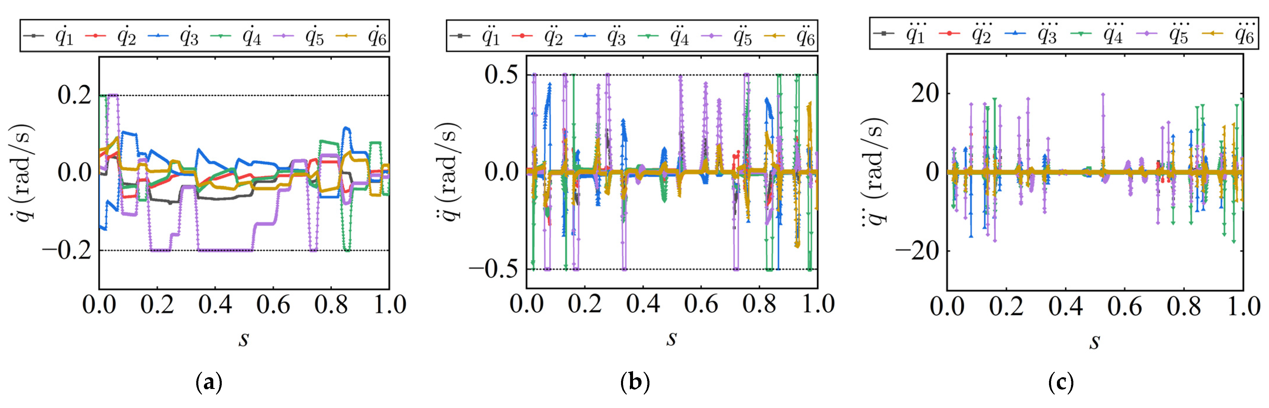
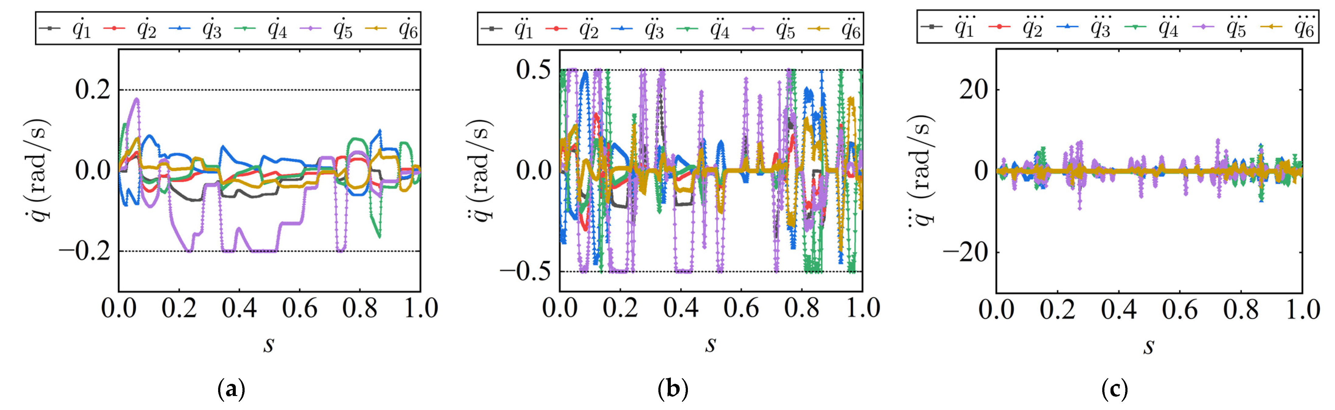
Figure 7 and
Figure 8 show the joint velocity, acceleration, and jerk profiles generated by the TOTP-2C and TOTP-2 methods. While both methods produce velocity curves with good continuity, the TOTP-2C method exhibits clear advantages in higher-order continuity. In particular, the acceleration and jerk profiles from TOTP-2C display smooth transitions at discrete points without noticeable discontinuities. In contrast, the acceleration and jerk profiles generated by the TOTP-2 method show abrupt changes at discrete points, especially in the jerk curve, which features sharp corners that indicate discontinuous behavior.
A further comparison of the jerk profiles generated by TOTP-2C and TOTP-2 shows that, although neither method applies jerk constraints and both share the same velocity and acceleration limits, the jerk variation range for TOTP-2C is approximately −9.17 to 7.66 rad/s3, while that for TOTP-2 reaches −17.46 to 19.75 rad/s3, indicating significantly larger fluctuations. This is mainly due to the fact that TOTP-2C produces a continuous and smoother acceleration profile, which leads to more gradual changes in acceleration and avoids abrupt transitions. As a result, the jerk values remain within a smaller and more stable range. Overall, the TOTP-2C method not only ensures higher-order continuity of the trajectory but also delivers superior smoothness, which helps to improve control performance and enhance the dynamic stability of the actuator during execution.
4.2. Validation of the Time-Jerk Multi-Objective Optimization Effectiveness
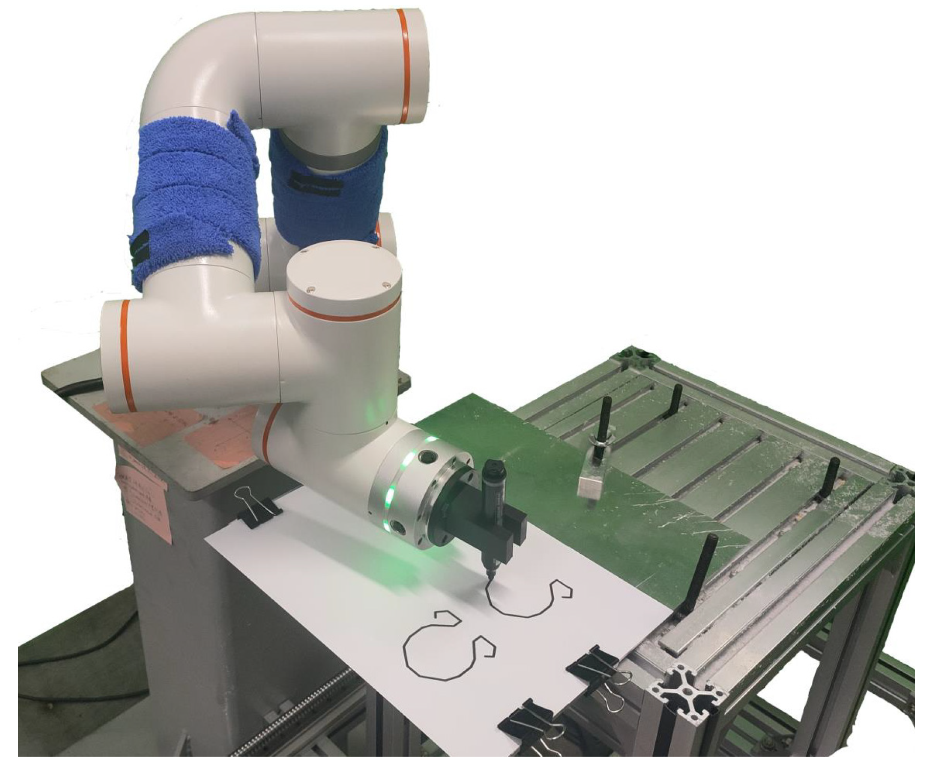
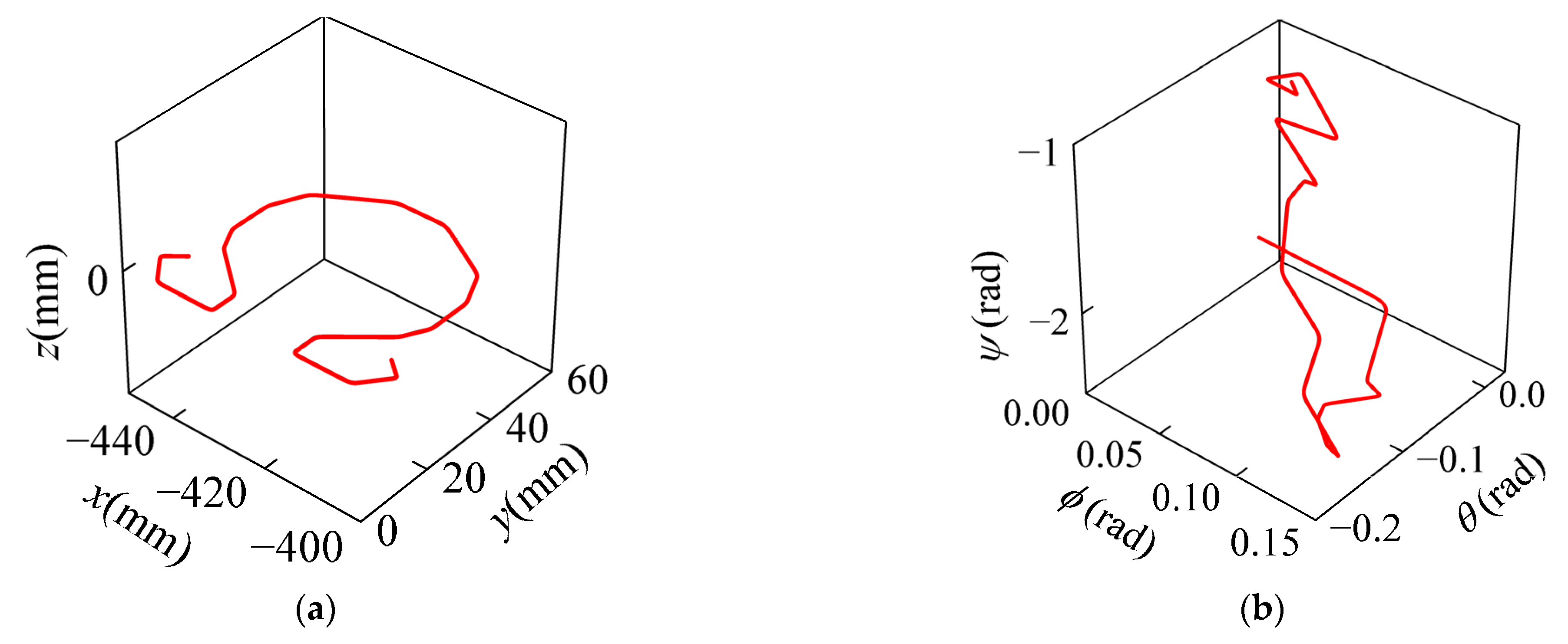
To assess the effectiveness of the proposed TJOTP-3C method in optimizing both execution time and joint jerk, the cosine-shaped EE path in
Figure 9 is selected for trajectory planning. The first-, second-, and third-order derivatives of the joint path with respect to the path parameter
s are shown in
Figure 10. The weighting factor
in the Equation (50) is assigned different values to examine its influence on the planning results. The TJOTP-3C method is applied for each setting. The discretization step size remains the same as in the previous experiment, and the constraint parameters are summarized in
Table 2.
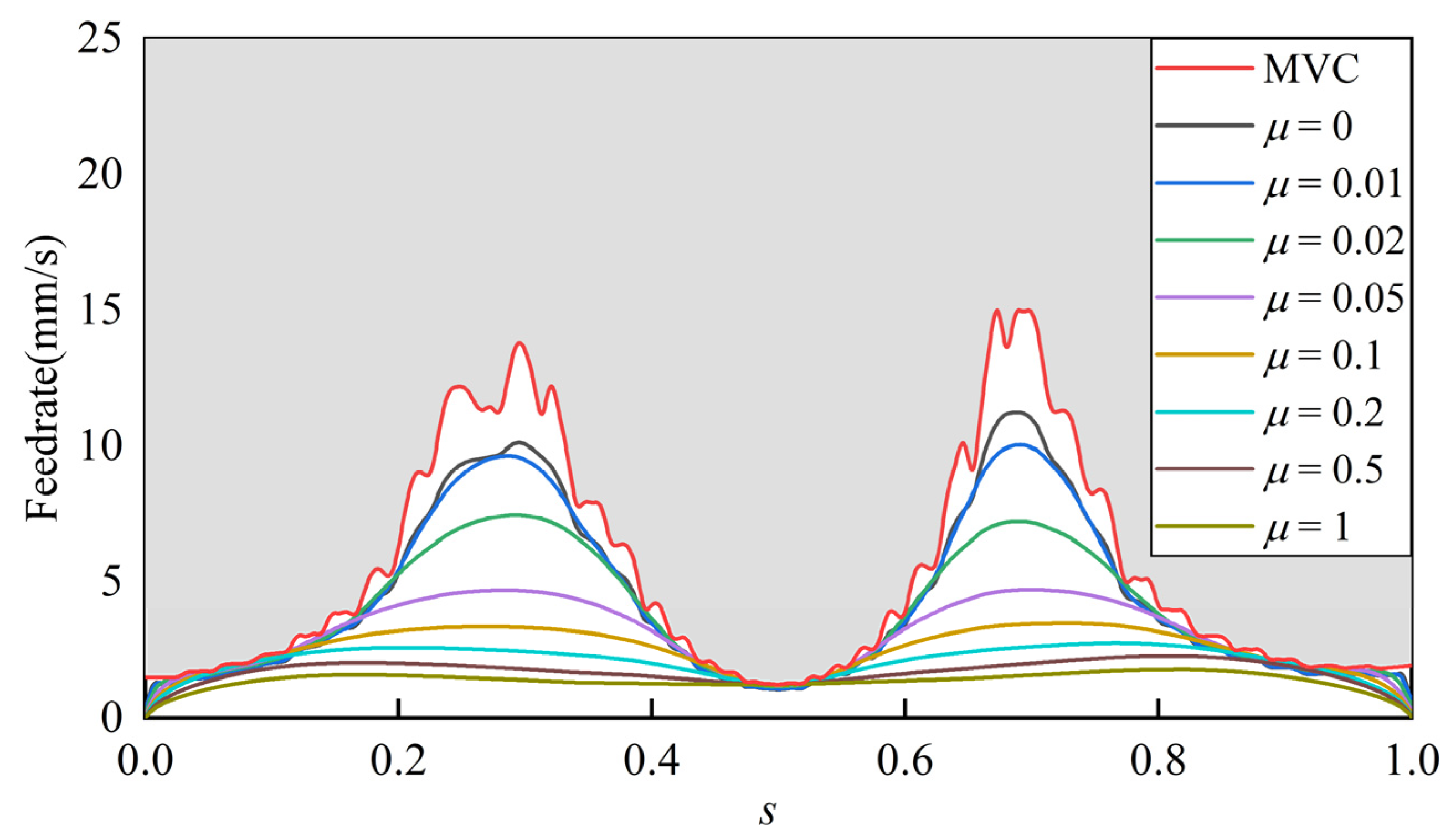
The feedrate profiles under different values of
are shown in
Figure 11, where MVC represents the maximum velocity curve considering joint velocity, joint acceleration, and EE feedrate constraints. As the value of
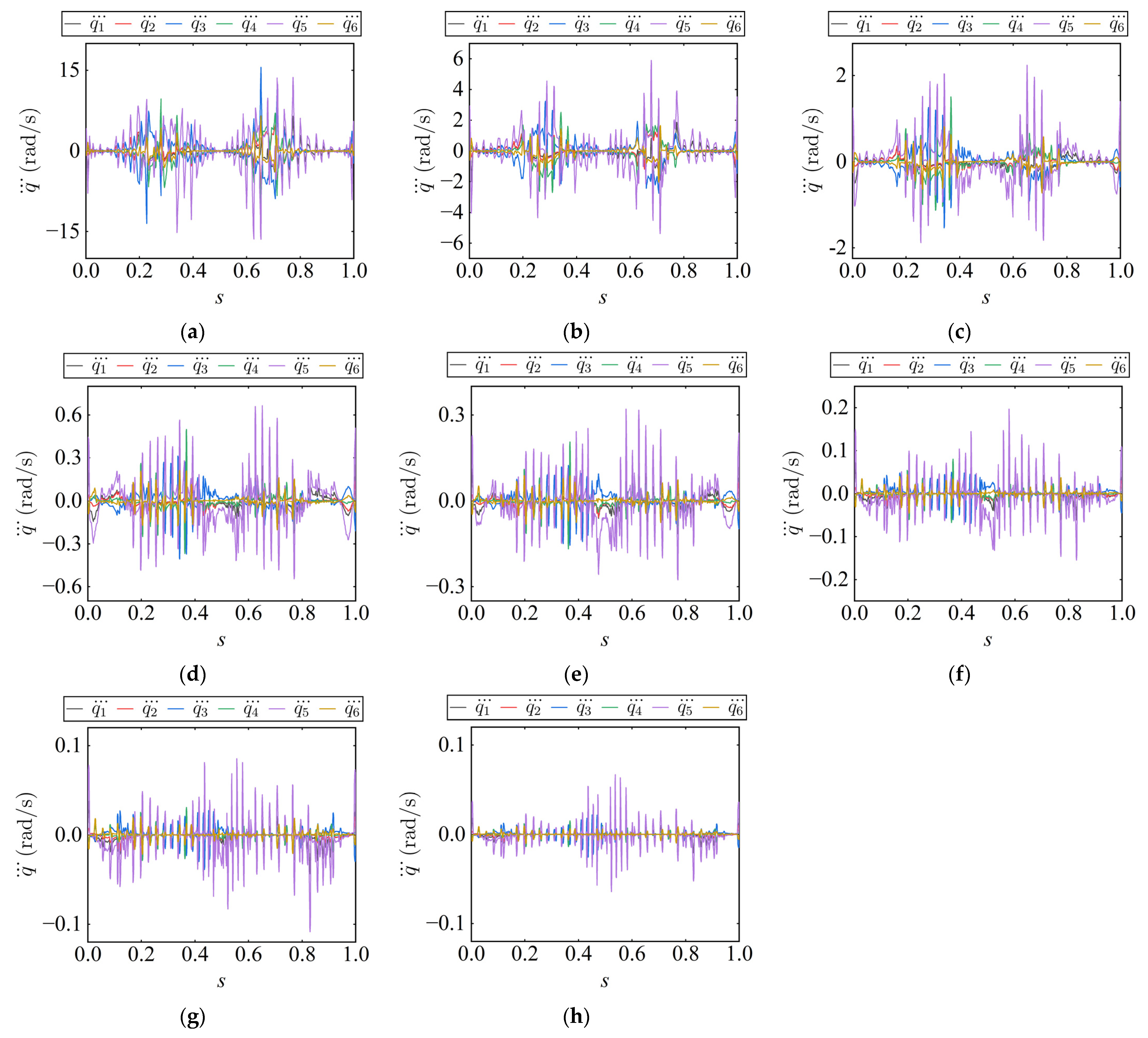
increases, the jerk evaluation term contributes more heavily to the objective function in TJOTP-3C, resulting in a lower feedrate but smoother velocity curves. The corresponding joint jerk profiles are also presented in
Figure 12. It can be clearly seen that increasing
leads to a gradual reduction in joint jerk, confirming the effectiveness of the jerk optimization strategy. This indicates that, beyond satisfying hard jerk constraints, the method can further suppress dynamic disturbances and enhance trajectory smoothness.
However, analysis of both the feedrate and jerk profiles reveals a trade-off. While a higher value of reduces joint jerk, it increases the trajectory execution time. This reflects the inherent conflict between time efficiency and jerk minimization. Therefore, in practical applications, the choice of should be determined based on the specific task requirements. For tasks with high demands on execution efficiency and relatively low sensitivity to motion-induced disturbances, such as robotic handling tasks, a smaller value of is more appropriate. For tasks where smooth motion is more critical and execution time is less of a concern, such as robotic milling, polishing, and other machining operations, a larger value of can be selected to reduce joint jerk and improve machining quality.
4.3. Validation of the TJOTP-3C Method via Method Comparison
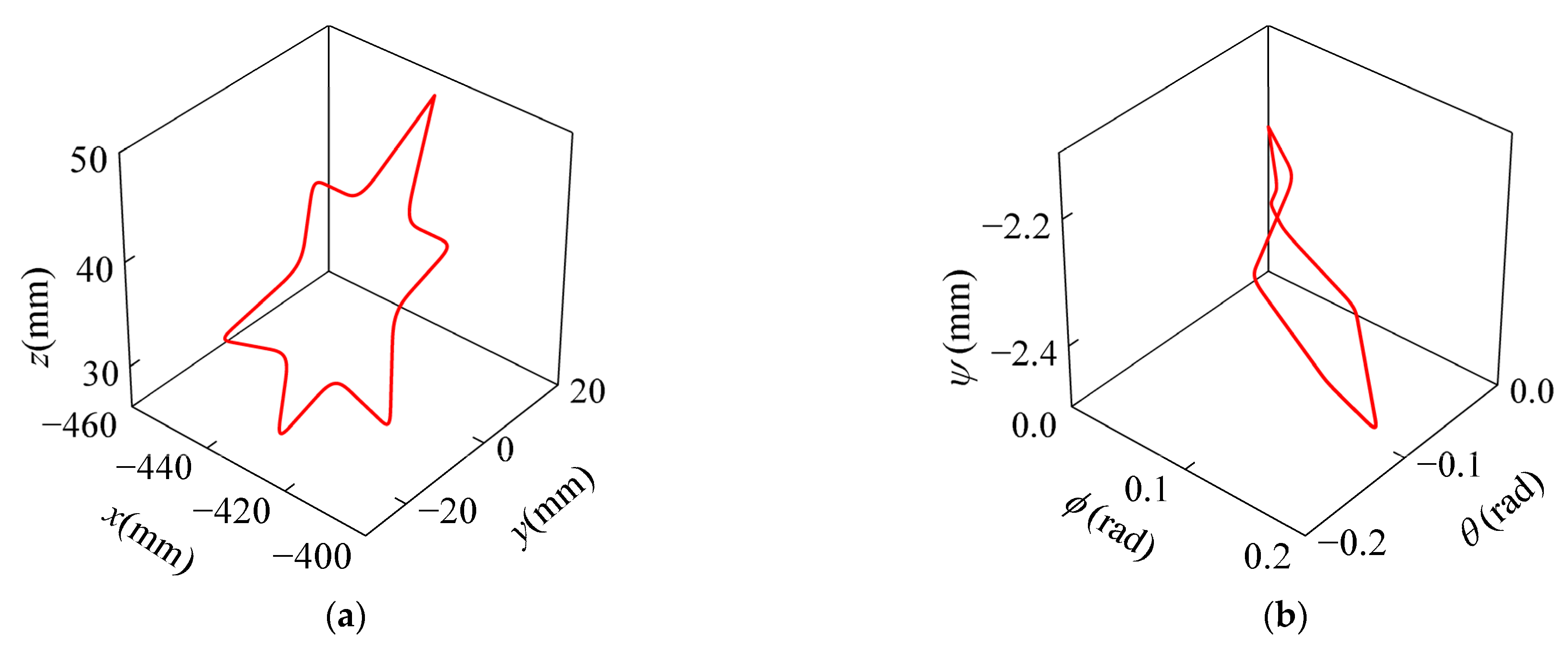
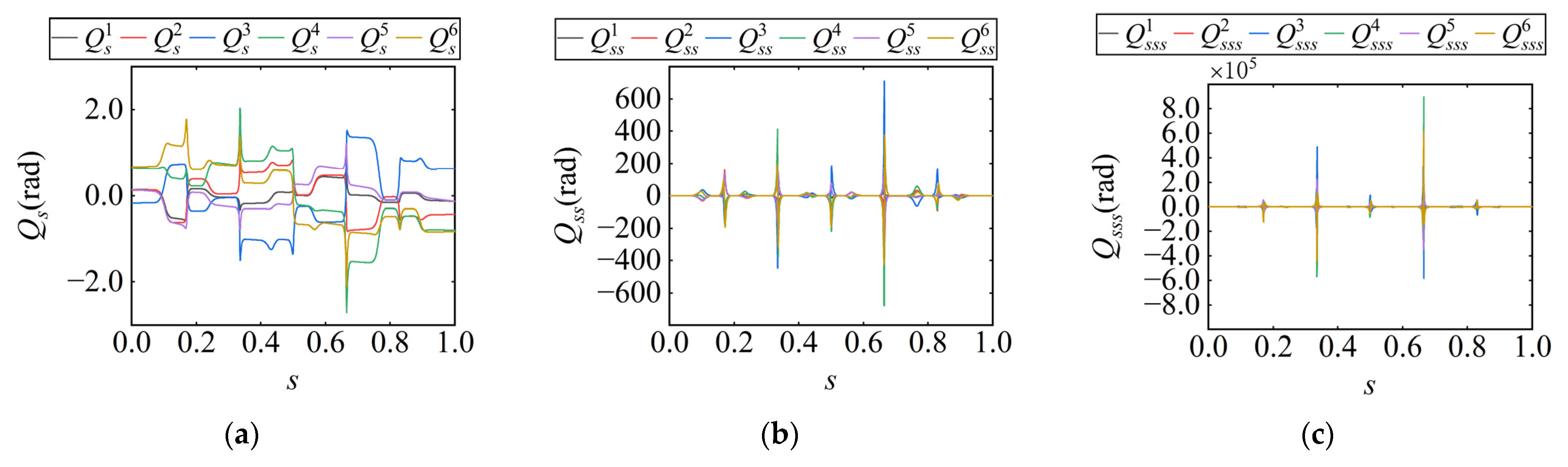
To evaluate the effectiveness of the proposed TJOTP-3C optimization method, trajectory planning is performed on the star-shaped path shown in
Figure 13 using the proposed approach. The first-, second-, and third-order derivatives of the joint path with respect to the path parameter “
s” are shown in
Figure 14. The kinematic and dynamic constraints in both the joint space and Cartesian space are defined as listed in
Table 3.
In the TJOTP-3C method, the path discretization parameters are kept consistent with those used in the previous two experiments. To demonstrate the advantages of the proposed approach, two other trajectory planning methods are selected for comparison. The first is the time-optimal trajectory planning method based on linear programming (TOTP-LP) proposed by Liu et al. [
23]. Although this method considers only constraints in joint space, it belongs to the class of convex optimization methods, similar to the proposed approach, and is therefore adopted as a comparison method to validate the effectiveness of the continuity constraints in TJOTP-3C. The second is a CBFS-based method proposed by Jia et al. [
37]. Ref [
37] defined regions where the maximum velocity curve falls below the commanded feedrate as velocity-sensitive regions. In these regions, the end-effector feedrate is kept constant. In contrast, S-curve acceleration and deceleration profiles are applied in non-sensitive regions to ensure smooth speed transitions. As CBFS is a representative feedrate scheduling strategy in trajectory planning, this method is used as another comparative approach. Originally designed for five-axis CNC machining without considering joint-space constraints, the method is adapted in this study by introducing the proportional adjustment strategy [
5] to ensure compatibility with joint kinematic constraints. In addition, the trigonometric acceleration and deceleration profile are used in place of the S-curve profile in Ref [
37] to achieve C
3 continuity in the trajectory.
Under identical constraints and sampling parameters, the trajectory of the star-shaped path is planned using the TJOTP-3C, TOTP-LP, and CBFS methods. To eliminate the influence of the jerk-related term in the TJOTP-3C objective function on the comparative analysis, the weighting factor is set to
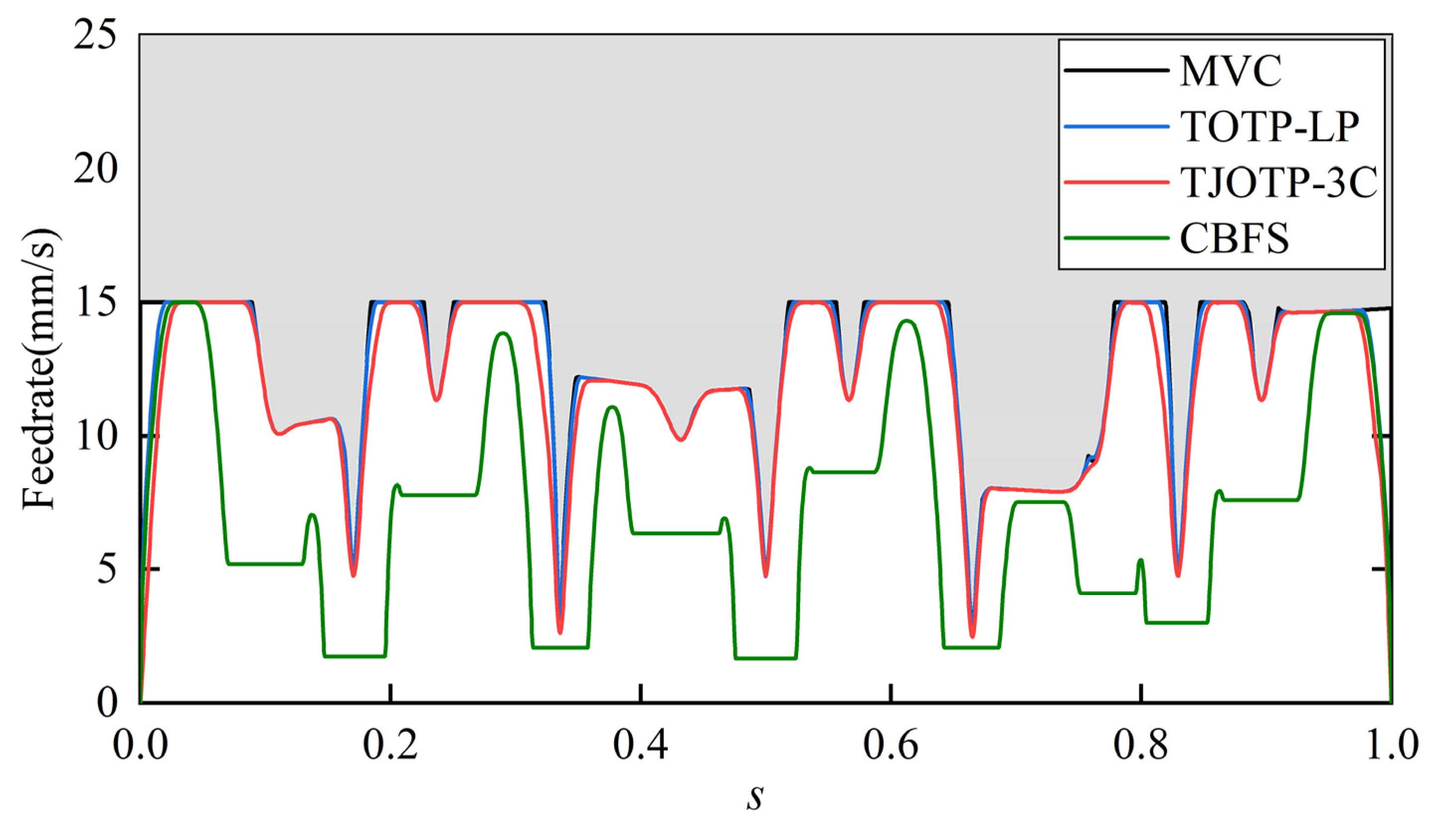
. The resulting feedrate profiles in Cartesian space for the three methods are shown in
Figure 15. In
Figure 15, MVC denotes the maximum velocity curve that satisfies joint velocity and acceleration constraints as well as the commanded feedrate of the end-effector. It can be observed that the feedrate profile generated by the TOTP-LP method is closest to the MVC, indicating that it achieves the highest trajectory execution efficiency. In contrast, the feedrate profiles generated by the TJOTP-3C and CBFS methods fall below that of TOTP-LP, suggesting longer overall execution. After mapping the trajectories from the parameter domain to the time domain, the trajectory durations for TOTP-LP, TJOTP-3C, and CBFS are 14.68 s, 15.23 s, and 36.76 s, respectively. Among the three methods, TOTP-LP yields the shortest duration, followed by TJOTP-3C, while CBFS results in the longest.
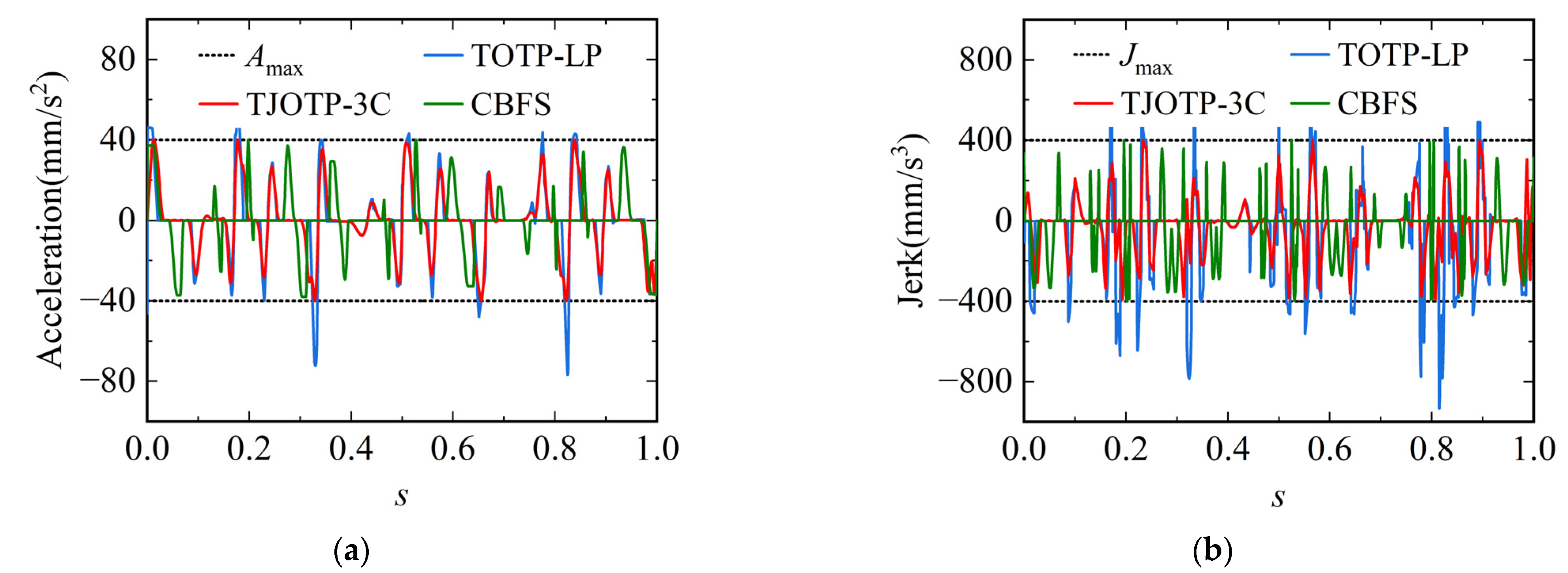
Although the TOTP-LP method provides higher trajectory execution efficiency, it imposes full kinematic and dynamic constraints only in the joint space. In the Cartesian space, TOTP-LP can constrain feedrate but lacks the ability to limit EE acceleration and jerk. As a result, the trajectory generated by TOTP-LP shows violations of the EE acceleration and jerk constraints, as illustrated in
Figure 16. In contrast, both the TJOTP-3C and CBFS methods apply full kinematic constraints in both joint and Cartesian spaces, ensuring that the end-effector velocity, acceleration, and jerk remain within their respective limits. Additionally, the TJOTP-3C method explicitly incorporates continuity constraints, while the CBFS method employs a trigonometric acceleration profile that is inherently C
3 continuous. These characteristics lead to smoother trajectories, which reduce jerk and vibration when compared to the C1 continuous trajectory produced by TOTP-LP.
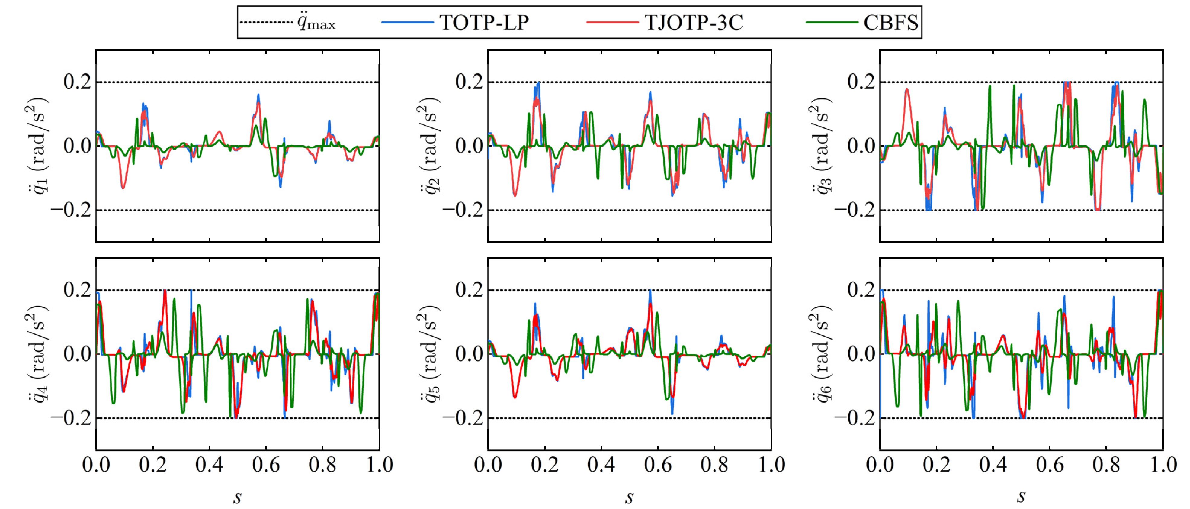
By applying inverse kinematics, the trajectories generated by the TOTP-LP, TJOTP-3C, and CBFS methods are transformed into joint space. The corresponding joint angular velocity, acceleration, and jerk profiles are shown in
Figure 17,
Figure 18 and
Figure 19, respectively. All three methods produce joint trajectories that satisfy the specified constraint limits, confirming the effectiveness of the compound constraint strategy proposed in this study.
As illustrated in
Figure 17, the joint velocity curves produced by the TOTP-LP and TJOTP-3C methods are nearly identical. This similarity arises from the fact that both methods are time-optimal and formulated using convex optimization. Aside from the EE acceleration, jerk, and continuity constraints uniquely imposed by TJOTP-3C, the two approaches share the same formulation, resulting in comparable trajectories. However, due to the absence of continuity constraints, the velocity profiles of TOTP-LP are less smooth, and its acceleration and jerk curves contain more pronounced sharp points. The CBFS method is inherently based on a C
3 continuous curve, naturally resulting in relatively smooth trajectories. However, it does not make full use of the joint kinematic constraints, which explains why its execution time is longer than that of both the TOTP-LP and TJOTP-3C methods. To quantitatively evaluate trajectory smoothness, the standard deviation (STD) values of joint velocity, acceleration, and jerk are reported in
Table 4. Benefiting from the enforcement of C
3 continuity, both CBFS and TJOTP-3C achieve lower RMS values than TOTP-LP across all motion levels, indicating smaller fluctuations and enhanced smoothness.
Taken as a whole, TJOTP-3C achieves more favorable results than the other two methods. The TOTP-LP method generates time-optimal trajectories but only ensures velocity continuity, resulting in limited smoothness that may lead to impacts and vibrations during execution. Moreover, it cannot constrain end-effector acceleration and jerk in Cartesian space. The CBFS method produces smoother, high-order continuous trajectories, but its velocity profile adjustment lacks flexibility and it does not support time optimization. As a result, it yields longer execution durations and lower machining efficiency. In addition, CBFS cannot incorporate the robot dynamic constraints. In contrast, TJOTP-3C accounts for a complete set of constraints in path-following tasks, supports execution time optimization, and generates smooth trajectories. From the perspectives of constraint completeness, execution time, and trajectory smoothness, TJOTP-3C provides a more balanced and effective solution than the other two methods. It not only inherits the time-optimization capability of TOTP-LP but also shares the ability of CBFS to generate smooth, high-order continuous trajectories.


