Robust Continuous Sliding-Mode-Based Assistive Torque Control for Series Elastic Actuator-Driven Hip Exoskeleton

Abstract

In this paper, a real-time assistive torque controller based on sliding-mode control is proposed for a Series Elastic Actuator (SEA)-driven lower limb assistive exoskeleton. To address the problem of the lack of buffering properties and the uneven torque output in traditional exoskeletons, a novel SEA is designed for the hip joint lower-limb exoskeleton. This structure features excellent cushioning properties and smooth torque output. On this basis, to enhance the torque tracking performance of the hip joint exoskeleton, in this study, a robust composite control strategy is proposed, which can maintain accuracy in the presence of unknown external disturbances and model parameter inaccuracies. The strategy consists of an adaptive phase oscillator for outputting the phase of the gait, a single-peak curve to provide a reference assistive torque, and a low-level controller to track the torque. The low-level controller employs Continuous Sliding-Mode Control (CSMC) to obtain a continuous control law and utilizes an Extended State Observer (ESO) to estimate the lumped disturbance. It ensures that the tracking error is asymptotically convergent with minimized chatter. The closed-loop stability of the system is theoretically proven by the Lyapunov method. The validity of the proposed algorithm is validated on a designed exoskeleton.

1. Introduction

In recent years, hip exoskeleton robots have been widely applied in fields such as walking assistance and motor rehabilitation to address the growing global issues related to aging populations and the increasing number of patients suffering from lower limb dysfunctions or loss due to factors like stroke, accidents, and spinal cord injuries [1,2,3]. As assistive devices, lower-limb exoskeleton robots can provide support and balance to patients who have lost their mobility, enabling them to walk normally [4,5]. Meanwhile, by synchronizing with the user’s movement, these exoskeletons can effectively assist in the rehabilitation of patients with movement injuries, enhancing muscle vitality and promoting the recovery of motor functions [6]. Flexibility, comfort, and safety are critical performance criteria for lower-limb rehabilitation robots [7], as these factors are essential to prevent secondary injuries resulting from human–robot interaction [8,9]. Therefore, designing compliant actuators for exoskeleton rehabilitation robots and using control algorithms to improve compliance and comfort is particularly important.

Notable advancements include a parallel hip exoskeleton with a telescopic motor drive that accommodates the human knee joint’s multi-center motion [10], the S-Assist gait-assistance exoskeleton for the elderly designed to conform to natural lower-limb curvature [11], and the QEPLEX wearable lower-limb exoskeleton featuring a motor-lasso hybrid drive system [12]. It is evident that all of the aforementioned factors serve to illustrate stable and efficient control. However, they are concomitantly encumbered by the disadvantage of excessive rotational inertia and mass. Gams et al. [13] proposed a rope-driven lower-limb exoskeleton with dual knee joints, which provides assistance when the user performs squatting actions. SCKAFOS [14] is a knee exoskeleton primarily designed for patients with polio, providing flexion force during the mid-swing phase of the leg and assisting with knee extension during the backward swing phase. The CALEX exoskeleton from Columbia University [15] helps the hip joint flex and extend using Bowden cables, enabling control of the wearer’s foot trajectory. The EU’s Xosoft [16] modular design provides $10\%$ assistance relative to natural forces, reducing energy consumption during walking. The Her team at MIT [17] proposed a rope-driven exoskeleton using a crank mechanism that reduces the wearer’s energy consumption by $11\%$. However, these exoskeletons use rigid actuators, resulting in a rough output and insufficiently smoothed assistance torque. To address the problem of the lack of buffering properties and the uneven torque output in traditional exoskeletons, a novel SEA is designed for the hip joint lower-limb exoskeleton. In terms of control, the introduction of SEA added some control challenges, which in turn rendered subsequent force-position control more difficult. Additionally, the human gait process is not a constant function curve, which introduces new challenges for gait profile adaptation and prediction.

Detecting the current gait phase is essential before outputting the assisting torque. Thus, acquiring a human’s motion intent and sensing exoskeleton motion are crucial research areas, which have inspired many scholars’ studies. For example, Xu et al. used an on-board training model to detect real-time gait events [18], Li’s study was the first to utilize heel and toe gaps for the online detection of all six gait events within a gait cycle [19], and Huang et al. performed walking detection based on a neural network [20]. Some studies have also used evolutionary algorithms [21] or machine learning [22,23] to adapt to environmental changes. From the above, it is clear that the use of appropriate algorithms to achieve dynamic adaptation of the exoskeleton to the gait is a universal choice. In this study, an adaptive phase oscillator is used to match the user’s movements, a method that has been proven effective in several studies [24,25,26].

In order to avoid human–machine confrontation and enhance the compliance of lower-limb rehabilitation robots, designing appropriate controllers to improve the comfort of exoskeleton robots has become an active research topic in recent years. Scholars have made various attempts to develop early control strategies for exoskeletons. Among them, adaptive control based on approximate dynamic programming has been applied to significantly improve gait asymmetry [27]. Additionally, some studies have adopted classical PD control while attempting to divide the gait process into multiple stages [28,29]. However, traditional trajectory tracking control algorithms in these studies still face issues such as slow response, noticeable oscillations, and large overshoot [30,31]. These algorithms are computationally heavy and suffer from significant output delays. Therefore, future research needs to further improve and optimize to better enhance the comfort of exoskeleton control.

Currently, various methods to improve the performance of flexible drive systems have been extensively studied, including singular perturbation control [32,33], feedback linearization control [34,35], backstepping control [36,37], neural network control [38], adaptive control [39], and Sliding-Mode Control (SMC) [40]. Among them, SMC has received widespread attention due to its ability to enhance system robustness through high-frequency switching terms and achieve global convergence quickly. However, the robustness of traditional sliding-mode control relies on the switching term gain being higher than the upper bound of composite disturbances, which may lead to significant chattering phenomena, thereby amplifying undesirable dynamic characteristics and affecting system performance, meaning they cannot be realized in practical applications. To address this issue, one study has proposed a sliding-mode control method [41], aimed at reducing control discontinuities. However, this method still results in a discontinuous control law. When significant uncertainties and disturbances are present, maintaining robustness still requires large switching term gains, which can still lead to chattering phenomena. The study proposed the continuous Sliding-Mode Control (CSMC) method to achieve continuous control [42], which replaces the sign function in the switching term with an integral of the sign function, thereby achieving continuous control and suppressing chattering. Conventional control strategies tend to be highly sensitive to the accuracy of parameters in order to ensure accuracy, but the measurement of system parameters is often subject to errors or changes during operation. In addition, the system needs to further improve the robustness. To address this issue, some SMC methods based on Disturbance Observer (DO) have been proposed, such as [43], along with CSMC based on Generalized Proportional-Integral Observer (GPIO) [44] and SMC based on Finite-Time Disturbance Observer (FTDO) [45]. These methods facilitate the incorporation of disturbance estimates derived from observations of the control law. This ensures that the switching term gain requirement is solely dependent on the upper limit of disturbance estimation error. The CSMC+ESO control strategy has received widespread attention as it inherits the advantages of ESO along with SMC’s high robustness while mitigating its shortcomings, particularly the issue of chattering.

The main contributions of this paper can be summarized in the following three parts.

In this study, an SEA mechanism with an adjustable bias angle is designed, which can change the stiffness characteristics by adjusting the radial arrangement angle of the tension spring. SEA has the advantages of soft output, adaptability, and comfort over traditional rigid actuators. This mechanism exhibits great linearity, and its operating range can accommodate the exoskeleton’s output moment range.

An adaptive oscillator is innovatively employed in the high-level controller to accurately acquire the gait phase and predict walking movements. Notably, this controller does not rely on enumerating specific walking states. Instead, the system itself approximates the walking cycle.

The low-level controller is controlled by a sliding-mode controller in conjunction with an extended state observer. The utilization of ESO facilitates system monitoring and the rectification of errors, significantly improving the robustness of the system. Concurrently, this study has been shown to enhance the efficacy of conventional sliding-mode control by substituting the sign function in the switching term with the integral of said function. The consequence of this modification is the attainment of a continuous control law, thereby effectively mitigating the occurrence of chattering.

2. Exoskeleton System

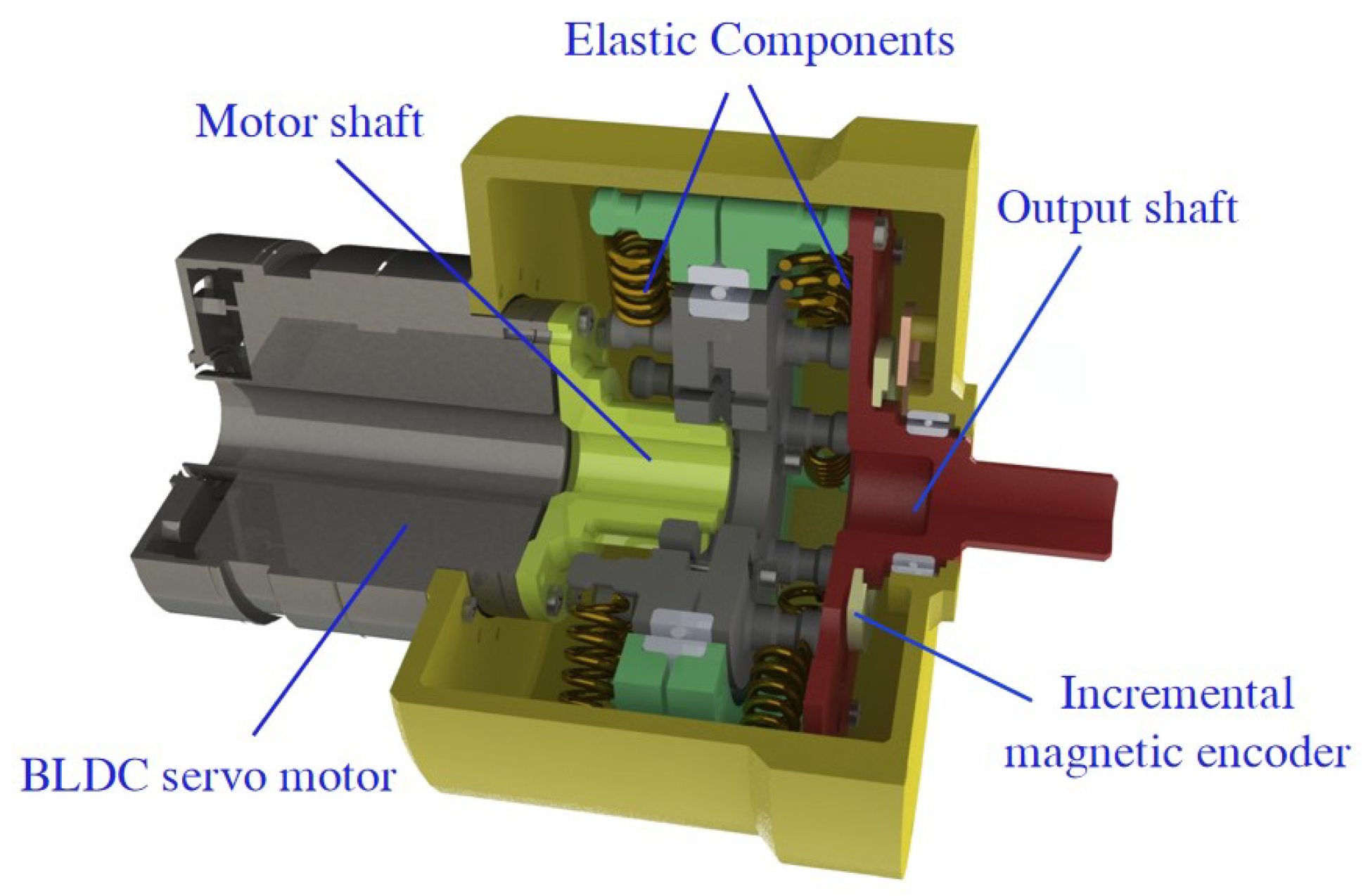
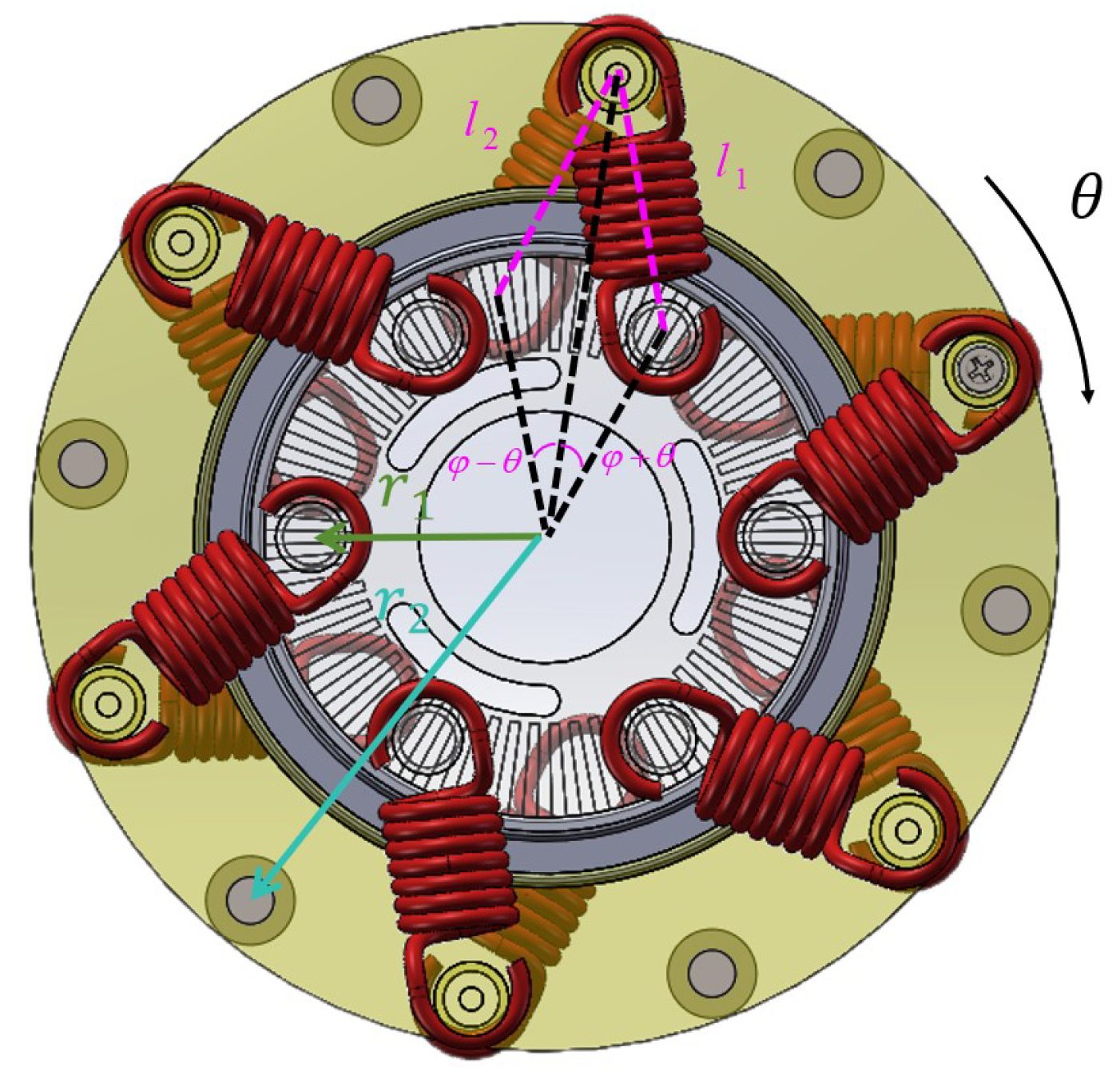
2.1. Design of Series Elastic Actuator

The schematic diagram of the mechanical structure of the SEA is shown in Figure 1, which consists of a Motor shaft, a BLDC servo motor, two sets of elastic components, an Output shaft, and an Incremental magnetic encoder. The fundamental principle of its design is that the output torque first passes through an elastic element before being transmitted to the user. Compared with rigid actuators, this mechanism significantly enhances the system’s interactive safety and comfort.

As shown in Figure 2, the designed SEA connects the motor end to the output end using an array of tension springs arranged radially along the circumference as the elastic elements, with six tension springs on each side, and these springs have radial bias angles. When the motor rotates, the end of the spring closer to the center of the circle is first pulled by the motor-end connector, and then the tension is transferred to the other end of the spring, which in turn drives the rotation of the output end. When the radial bias angle of the spring is varied, the stiffness characteristics of the SEA also change correspondingly. In order to adjust the designed SEA to the most suitable stiffness characteristics according to the actual situation, the motor-end connector is designed with a toothed groove structure, and the angle between two adjacent teeth on the same side of the tooth surface is 6 degrees. Therefore, the radial bias angle of the spring can be adjusted from 0 degrees to 60 degrees in increments of 6 degrees. After derivation, the following mechanical properties of the designed SEA are obtained:

$$\left\{\begin{array}{c}{L}_1=\sqrt{{r_1}^2+{r_2}^2-2r_1{r}_{2}cos\left(\varphi -\mathsf{\Theta }\right)}\hfill \\ L_2=\sqrt{{r_1}^2+{r_2}^2-2r_1{r}_{2}cos\left(\varphi +\mathsf{\Theta }\right)}\hfill \\ {\tau }_s=6k_s{r}_1{r}_2\hfill \\ \left(\left(1-{\displaystyle \frac{L_0}{L_2}}\right)sin\left(\varphi +\mathsf{\Theta }\right)-\left(1-{\displaystyle \frac{L_0}{L_1}}\right)sin\left(\varphi -\mathsf{\Theta }\right)\right)\hfill \end{array}\right.$$

(1)

where ${\tau }_s$ is the output torque of SEA and $r_1$ and $r_2$ are the rotation radii of the two ends of the spring, respectively. $\varphi$ is the radial arrangement angle and $\mathsf{\Theta }$ is the angle difference between the inner and outer disks, i.e., the elastic deformation variable. $L_0$ is the original length of the spring and $k_s$ is the spring stiffness.

By recording the output torque and elastic deformation of the SEA in real-time, the stiffness characteristics of the designed SEA are shown in Figure 3, which exhibit good linearity and low hysteresis. By linear fitting, the equivalent stiffness is obtained as 1.047 Nm/deg.

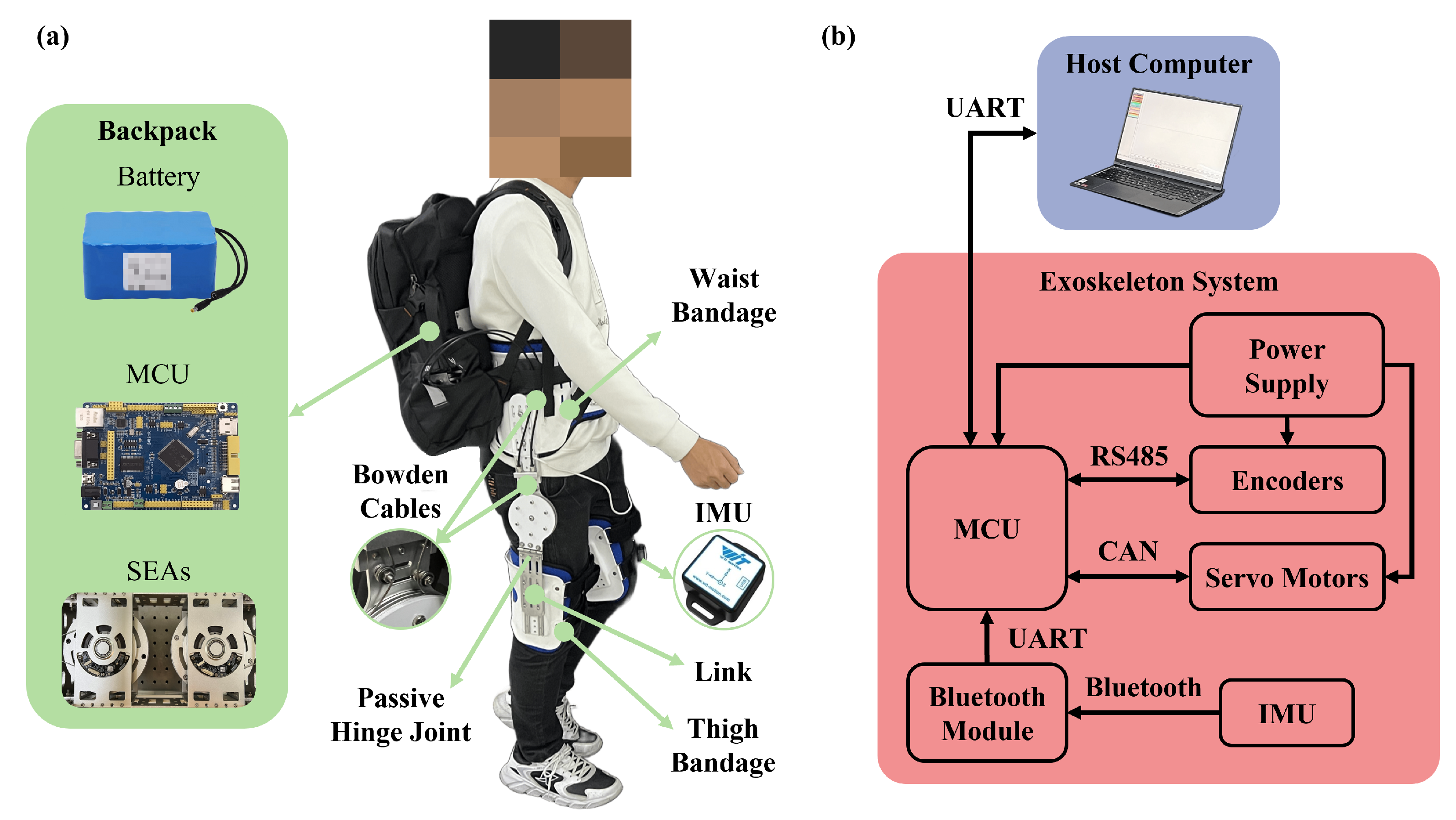
2.2. Exoskeleton System Design

The hip exoskeleton used in this study is shown in Figure 4, which mainly consists of a pair of SEAs, a set of rope-driven systems, a ligature device, and a measurement and control system. The exoskeleton system is driven by the rope drive system, which is secured to the user’s body by a ligature device and transmits torque to the hip joint. The measurement control system contains two 9-axis IMUs (WT901SDCL-BT50, WIT, Guangdong, China) that transmit hip joint angle and angular velocity signals to the control board via Bluetooth at 200 Hz.

2.3. Electronics and Control Implementation

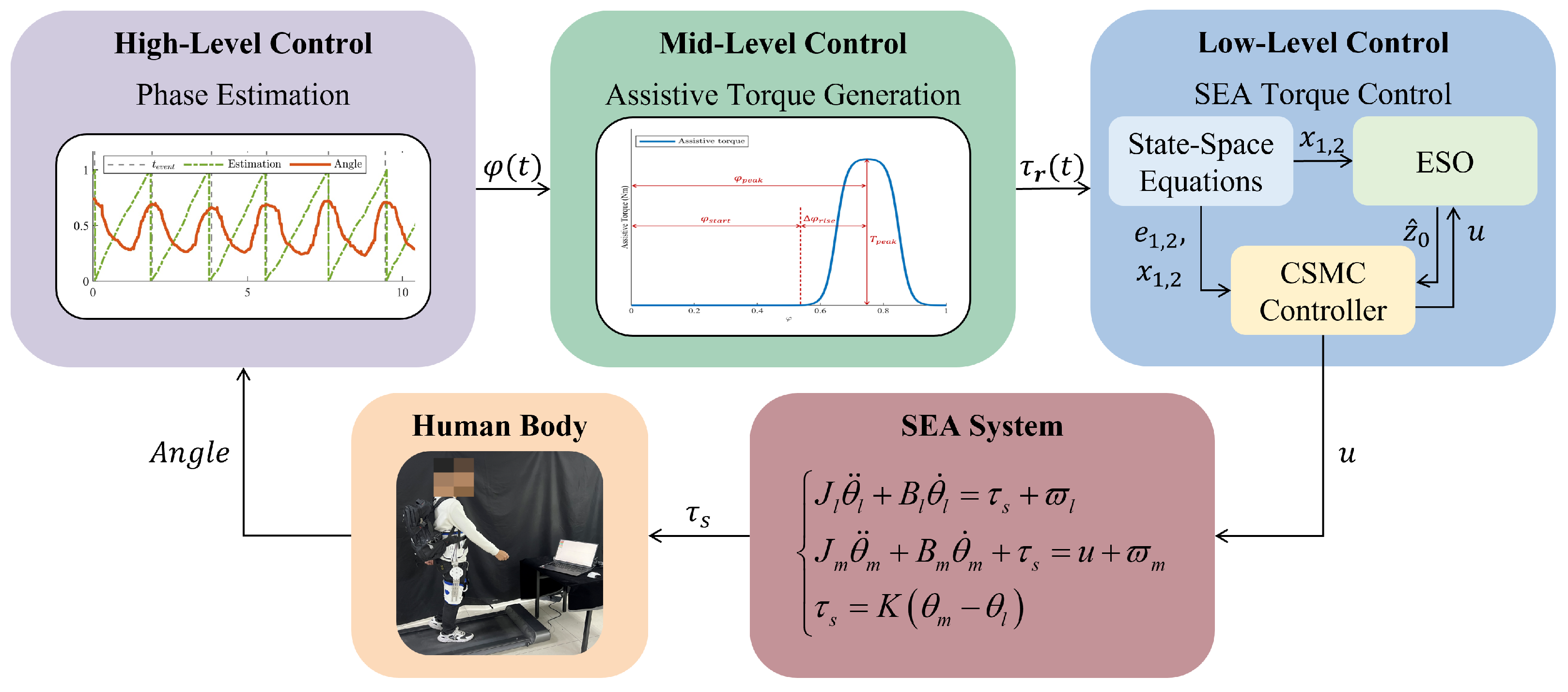
The electrical system is depicted in Figure 4, receiving data from the IMU (±0.2° static attitude error, ±20∼40 mg accelerometer zero-bias, 0.75 mg-rms noise, ±0.5°/s gyro zero-bias); a Bluetooth-to-serial conversion module (MX-02, MIAOSHARE, Shenzhen, China) was used as the communication medium in this study. The control board processes the data received and sends control signals to the motors. As the power source of the exoskeleton, each SEA is powered by a DC brushless servomotor (CRA-RI60-70-PRO, TI5 ROBOT, Shanghai, China) to provide an average maximum driving torque of 32 Nm, with a CAN communication period of 1 ms. To achieve closed-loop control, the position and velocity of the SEA outputs need to be measured. An absolute magnetic encoder (eCoder35, 17-bit resolution, ZEROERR, Shenzhen, China) is used for this purpose. The encoder communicates via RS485 and sends the measured data to the control board.

3. Control Strategy

The adaptive phase oscillator-based control strategy is depicted in Figure 5. The control strategy consists of three parts: high-level, mid-level, and low-level control. The high-level controller is responsible for detecting the user’s gait period and current phase, and employs an adaptive phase oscillator to provide real-time estimation of the linear gait phase. The mid-level controller converts the phase signal into a desired assist torque signal based on a single-peak curve with parameters. The low-level controller integrates a continuous sliding-mode controller with an extended state observer to control the actuator’s output torque, ensuring that the output torque tracks the ideal assist torque. This study focuses on the development and implementation of the high-level and low-level control strategies.

3.1. High-Level Control

In this study, a high-level controller employing an adaptive phase oscillator is used to estimate the gait phase of the user’s quasi-periodic walking motion, thereby facilitating the subsequent determination of the corresponding control input. Human walking is inherently non-periodic, with variations in step frequency and step length across gait cycles. This variability in human walking necessitates real-time estimation of the gait phase based on sensor signals to enable intelligent assistance. To address this challenge, an adaptive phase oscillator is introduced to estimate the gait phase accurately in real time. The input to this system is the rotational angular velocity signal from the IMU module. The adaptive phase oscillator [46] is described by the following equation:

$$\begin{array}{c}{\dot{\phi }}_0=\omega -\psi e\left(t\right)cos\left({\phi }_0\right)\hfill \\ \dot{\omega }=-\psi e\left(t\right)cos\left({\phi }_0\right)\hfill \\ {\dot{\alpha }}_k=\epsilon cos\left(k{\phi }_0\right)e\left(t\right),\left(k=0,\dots ,N_f\right)\hfill \\ {\dot{\beta }}_k=\epsilon sin\left(k{\phi }_0\right)e\left(t\right),\left(k=0,\dots ,N_f\right)\hfill \\ \widehat{\dot{\theta }}={\displaystyle \sum _{k=0}^{N_f}}{\alpha }_{k}cos\left(k{\phi }_0\right)+{\beta }_{k}sin\left(k{\phi }_0\right)\hfill \end{array}$$

(2)

where ${\phi }_0$ is the original gait phase estimation, $\omega$ is the intrinsic frequency of the oscillator, $\psi$ and $\epsilon$ are the learning gains of the oscillator, $\widehat{\dot{\theta }}$ is the hip angular velocity estimation, and $e\left(t\right)=\dot{\theta }\left(t\right)-\widehat{\dot{\theta }}\left(t\right)$ is the error in angular velocity estimation, which is the driving source of the oscillator.

After obtaining the original gait phase estimate, it is normalized to $\left[0,2\pi \right)$

$${\phi }_{ao}\left(t\right)=mod\left({\phi }_0\left(t\right),2\pi \right)$$

(3)

At this point, ${\phi }_{ao}$ is the final output of the gait phase estimated by the oscillator.

Despite the use of an adaptive oscillator, the user’s gait period remains inherently uncertain, rendering the phases described by the equation ${\phi }_{ao}\left(t\right)$ not directly applicable. To address the misalignment between cycles, the onset of each gait cycle must be precisely defined, and the phase should be recalibrated by resetting it to zero at that moment. Ideally, the estimated gait phases should increase linearly from 0 to 1, with 0 corresponding to the initiation of each gait cycle. For hip exoskeletons, the most commonly used start marker is the maximum hip flexion and extension, an event that can be readily detected. When a characteristic gait event is detected, the amount of mismatch can be calculated from the following equation

$$P_e\left(t_{event}\right)=\left\{\begin{array}{c}-{\phi }_{ao}\left(t_{event}\right),{\phi }_{ao}\in \left[0,\pi \right)\hfill \\ 2\pi -{\phi }_{ao}\left(t_{event}\right),{\phi }_{ao}\in \left[\pi ,2\pi \right)\hfill \end{array}\right.$$

(4)

The mismatch is then corrected by the following equation to synchronize the phase estimate with the wearer’s gait

$$\left\{\begin{array}{c}{\dot{\delta }}_{\phi }=K_{\phi }\left(P_e\left(t_{event}\right)+{\delta }_{\phi }\right)e^{-\omega \left(t\right)\left(t-t_{event}\right)}\hfill \\ \phi \left(t\right)=mod\left({\phi }_{ao}\left(t\right)+{\delta }_{\phi }\left(t\right),2\pi \right)\hfill \end{array}\right.$$

(5)

where $K_{\phi }$ is the proportional gain, $t_{event}$ is the moment when the last characteristic event is detected, and $\phi$ is the corrected gait phase estimate. When the phase is synchronized, the start of each gait cycle is then locked to the characteristic gait event.

3.2. Mid-Level Control

After obtaining the user’s phase estimate, the mid-level controller needs to convert the phase information into the assisting torque required by the user, determining the assisting torque required by the user at different moments in the cycle. The mid-level controller of the exoskeleton uses a parametric single-peak curve [47], as shown in Figure 6, with the following equation:

$$f(\phi ,{\phi }_{start},T_{peak})={\displaystyle \frac{T_{peak}}{2}}(tanh(\gamma (\zeta (\phi ,{\phi }_{start})-{\displaystyle \frac{1}{2}}))-tanh(\gamma (\zeta (\phi ,{\phi }_{start})-{\displaystyle \frac{3}{2}})))$$

(6)

where ${\phi }_{start}$ is the phase at which the boost starts to intervene, $T_{peak}$ is the peak of the boost, and $\gamma$ is a positive constant that mainly affects the smoothness of the curve.

$$\zeta (\phi ,{\phi }_{start})={\displaystyle \frac{\phi -{\phi }_{start}}{\Delta {\phi }_{rise}}}$$

(7)

is a function of $\phi$, where $\Delta {\phi }_{rise}$ is the phase interval at which the assistance curve rises.

3.3. Low-Level Control

The low-level controller receives the assistive torque curve from the mid-level controller and uses a composite CSMC strategy to control the SEA to track the curve. The composite CSMC consists of the CSMC and the ESO.

3.3.1. SEA Drive

According to ref. [48], the dynamics of the SEA can be described as

$$\left\{\begin{array}{c}{J}_l{\ddot{\theta }}_l+B_l{\dot{\theta }}_l={\tau }_s+{\varpi }_l\hfill \\ J_m{\ddot{\theta }}_m+B_m{\dot{\theta }}_m+{\tau }_s=u+{\varpi }_m\hfill \\ {\tau }_s=K({\theta }_m-{\theta }_l)\hfill \end{array}\right.$$

(8)

where ${\theta }_m$ and ${\theta }_l$ are the angular positions of the actuator end and the load end, respectively, K is the equivalent stiffness of the elastic link, $J_m$ is the rotational moment of inertia of the actuator end, ${\tau }_m$ is the output moment of the actuator, $B_m$ is the damping of the motion, ${\varpi }_m$ is the unknown external perturbation of the actuator end, ${\tau }_s$ is the load moment, and ${\varpi }_l$ is the unknown external perturbation of the load end.

To define the output of the actuator, (8) is converted to

$$J_m({\ddot{\theta }}_m-{\ddot{\theta }}_l)+B_m({\dot{\theta }}_m-{\dot{\theta }}_l)+K({\theta }_m-{\theta }_l)=u+{\varpi }_m-J_m{\ddot{\theta }}_l-B_m{\dot{\theta }}_l$$

(9)

Letting $x_2={\dot{\theta }}_m-{\dot{\theta }}_l$, (9) can be written as

$$J_m{\dot{x}}_2+B_m{x}_2+K{x}_1=u+{\varpi }_m-J_m{\ddot{\theta }}_l-B_m{\dot{\theta }}_l$$

(10)

Considering the uncertainty in the model parameters in practice, the following parameter is introduced.

$$\begin{array}{c}{J}_m=J_{m0}+\Delta J_m\hfill \\ B_m=B_{m0}+\Delta B_m\hfill \end{array}$$

(11)

where $J_{m0}$ and $B_{m0}$ are the the nominal parameters of the moment of inertia and motion damping at the actuator end and $\Delta J_m$ and $\Delta B_m$ are the uncertainties of the moment of inertia and motion damping at the actuator end, respectively.

From the above, (10) can be transformed into

$$J_{m0}{\dot{x}}_2+B_{m0}{x}_2+K{x}_1=u+d$$

(12)

Let the lumped disturbance of the system be

$$d={J_{m0}}^{-1}({\varpi }_m-J_m{\ddot{\theta }}_l-B_m{\dot{\theta }}_l-\Delta J_m{\dot{x}}_2-\Delta B_m{x}_2)$$

(13)

Then, the state space equation of the system is derived as

$$\begin{array}{c}\left\{\begin{array}{c}{\dot{x}}_1=x_2\hfill \\ {\dot{x}}_2={J_{m0}}^{-1}(u-B_{m0}{x}_2-K{x}_1)+d\hfill \end{array}\right.\hfill \end{array}$$

(14)

The ${\tau }_r\in R$ denotes the trajectory of the input torque of the SEA, while ${\tau }_s=K{x}_1$ is the output torque of the SEA. The error dynamics equation is defined as follows:

$$\left\{\begin{array}{c}{e}_1={\tau }_r-{\tau }_s={\tau }_r-K{x}_1\hfill \\ e_2={\dot{\tau }}_r-{\dot{\tau }}_s={\dot{\tau }}_r-K{x}_2\hfill \\ {\dot{e}}_2={\ddot{e}}_1={\ddot{\tau }}_r-K[{J_{m0}}^{-1}(u-B_{m0}{x}_2-K{x}_1)+d]\hfill \end{array}\right.$$

(15)

3.3.2. Extended State Observer

The robustness of exoskeleton systems is a primary design metric. In order to enhance the robustness of exoskeleton control strategies, previous approaches have either overlooked the impact of operational errors or have relied on robust, perturbation-insensitive control methods. However, these approaches have typically resulted in a compromise between accuracy and response speed. The present study introduces an ESO to estimate the error magnitude. By tuning control based on this estimation, system accuracy and robustness can be enhanced without compromising response speed. The primary focus here is on errors caused by external disturbance torques and system parameter uncertainties. In order to set the ESO, let $z_0=d$ and $z_1=\dot{d}$. According to (14), the following delineation is provided for the purpose of illustrating the configuration of an ESO:

$$\left\{\begin{array}{c}{\dot{\widehat{x}}}_1={\widehat{x}}_2-{\lambda }_1({\widehat{x}}_1-x_1)\hfill \\ {\dot{\widehat{x}}}_2={J_{m0}}^{-1}(u-B_{m0}{x}_2-K{x}_1)+{\widehat{z}}_0-{\lambda }_2({\widehat{x}}_1-x_1)\hfill \\ {\widehat{z}}_0=-{\lambda }_3({\widehat{x}}_1-x_1)\hfill \end{array}\right.$$

(16)

where ${\lambda }_1$, ${\lambda }_2$, ${\lambda }_3$ are the gains of the ESO and ${\widehat{x}}_1$, ${\widehat{x}}_2$, ${\widehat{z}}_0$ are estimates of $x_1,x_2,z_0$ by the system observer, respectively.

Defining the error as ${\tilde{x}}_1$, ${\tilde{x}}_2$, ${\tilde{z}}_0$, we can obtain the following equation: ${\tilde{x}}_1={\widehat{x}}_1-x_1$, ${\tilde{x}}_2={\widehat{x}}_2-x_2$, ${\tilde{z}}_0={\widehat{z}}_0-z_0$, and we obtain:

$$\left\{\begin{array}{c}{\dot{\tilde{x}}}_1=-{\lambda }_1{\tilde{x}}_1+{\tilde{x}}_2\hfill \\ {\dot{\tilde{x}}}_2=-{\lambda }_2{\tilde{x}}_1+{\tilde{z}}_0\hfill \\ {\dot{\tilde{z}}}_0=-{\lambda }_3{\tilde{x}}_1-z_1\hfill \end{array}\right.$$

(17)

Theorem 1. 

It can be demonstrated that, under the condition that the appropriate gains ${\lambda }_i(i=1,2,3)$, it is possible to guarantee the stability of the system (18). It is expected that observer error, represented by ${\mathbf{E}}_{\mathsf{\Lambda }}$, will be reduced to an arbitrarily small range that encompasses the original point.

$$\epsilon =\left\{{\mathbf{E}}_{\mathsf{\Lambda }}|∥{\mathbf{E}}_{\mathsf{\Lambda }}∥\le {\displaystyle \frac{2{\lambda }_{max}\left(\mathbf{P}\right)∥\mathbf{PD}∥}{{\lambda }_{min}\left(\mathbf{Q}\right){\lambda }_{min}\left(\mathbf{P}\right)}}\right\}$$

(18)

Proof of Theorem 1. 

Letting ${\mathbf{E}}_{\mathsf{\Lambda }}=\left[{\tilde{x}}_1,{\tilde{x}}_2,{\tilde{z}}_0\right]$, the state space equation for the observation error is

$${\dot{\mathbf{E}}}_{\mathsf{\Lambda }}=\mathbf{A}{\mathbf{E}}_{\mathsf{\Lambda }}+\mathbf{D}$$

(19)

Select the Lyapunov function:

$$V\left({\mathbf{E}}_{\mathsf{\Lambda }}\right)={{\mathbf{E}}_{\mathsf{\Lambda }}}^T\mathbf{P}{\mathbf{E}}_{\mathsf{\Lambda }}$$

(20)

The time-derivative can be expressed as such:

$$\begin{array}{c}\dot{V}\left({\mathbf{E}}_{\mathsf{\Lambda }}\right)={\dot{\mathbf{E}}}_{\mathsf{\Lambda }}^T\mathbf{P}{\mathbf{E}}_{\mathsf{\Lambda }}+{{\mathbf{E}}_{\mathsf{\Lambda }}}^T\mathbf{P}{\dot{\mathbf{E}}}_{\mathsf{\Lambda }}\hfill \\ ={\left(\mathbf{A}{\mathbf{E}}_{\mathsf{\Lambda }}+\mathbf{D}\right)}^T\mathbf{P}{\mathbf{E}}_{\mathsf{\Lambda }}+{{\mathbf{E}}_{\mathsf{\Lambda }}}^T\mathbf{P}\left(A{\mathbf{E}}_{\mathsf{\Lambda }}+\mathbf{D}\right)\hfill \\ =-{{\mathbf{E}}_{\mathsf{\Lambda }}}^T\mathbf{Q}{\mathbf{E}}_{\mathsf{\Lambda }}+2{{\mathbf{E}}_{\mathsf{\Lambda }}}^T\mathbf{PD}\hfill \\ \le -{\lambda }_{min}\left(\mathbf{Q}\right){∥{\mathbf{E}}_{\mathsf{\Lambda }}∥}^2+2∥{\mathbf{E}}_{\mathsf{\Lambda }}∥·∥\mathbf{PD}∥\hfill \end{array}$$

(21)

Since P is a positive definite matrix and ${\mathbf{P}}^T=\mathbf{P}$, the following equation can be obtained:

$${\lambda }_{min}\left(\mathbf{P}\right){∥{\mathbf{E}}_{\mathsf{\Lambda }}∥}^2\le V\left({\mathbf{E}}_{\mathsf{\Lambda }}\right)={{\mathbf{E}}_{\mathsf{\Lambda }}}^T\mathbf{P}{\mathbf{E}}_{\mathsf{\Lambda }}\le {\lambda }_{max}\left(\mathbf{P}\right){∥{\mathbf{E}}_{\mathsf{\Lambda }}∥}^2$$

(22)

Equation (22) can be simplified as the following equation:

$$\sqrt{{\displaystyle \frac{V\left({\mathbf{E}}_{\mathsf{\Lambda }}\right)}{{\lambda }_{max}\left(\mathbf{P}\right)}}}\le ∥{\mathbf{E}}_{\mathsf{\Lambda }}∥\le \sqrt{{\displaystyle \frac{V\left({\mathbf{E}}_{\mathsf{\Lambda }}\right)}{{\lambda }_{min}\left(\mathbf{P}\right)}}}$$

(23)

Substituting (23) into (21), we obtain following equation:

$$\dot{V}\left({\mathbf{E}}_{\mathsf{\Lambda }}\right)\le -{\lambda }_{min}\left(\mathbf{Q}\right){\displaystyle \frac{V\left({\mathbf{E}}_{\mathsf{\Lambda }}\right)}{{\lambda }_{max}\left(\mathbf{P}\right)}}+2∥\mathbf{PD}∥\sqrt{{\displaystyle \frac{V\left({\mathbf{E}}_{\mathsf{\Lambda }}\right)}{{\lambda }_{min}\left(\mathbf{P}\right)}}}$$

(24)

Since ${\displaystyle \frac{d\sqrt{V\left({\mathbf{E}}_{\mathsf{\Lambda }}\right)}}{dt}}={\displaystyle \frac{\dot{V}\left({\dot{\mathbf{E}}}_{\mathsf{\Lambda }}\right)}{2\sqrt{V\left({\dot{\mathbf{E}}}_{\mathsf{\Lambda }}\right)}}}$, it follows that:

$${\displaystyle \frac{d\sqrt{V\left({\mathbf{E}}_{\mathsf{\Lambda }}\right)}}{dt}}\le -{\displaystyle \frac{{\lambda }_{min}\left(\mathbf{Q}\right)}{2{\lambda }_{max}\left(\mathbf{P}\right)}}\sqrt{V\left({\mathbf{E}}_{\mathsf{\Lambda }}\right)}+{\displaystyle \frac{∥\mathbf{PD}∥}{\sqrt{{\lambda }_{min}\left(\mathbf{P}\right)}}}$$

(25)

The above equation can be solved as the following equation:

$$\begin{array}{c}\sqrt{V\left({\mathbf{E}}_{\mathsf{\Lambda }}\right)}\le {\displaystyle \frac{2{\lambda }_{max}\left(\mathbf{P}\right)∥\mathbf{PD}∥}{{\lambda }_{min}\left(\mathbf{Q}\right)\sqrt{{\lambda }_{min}\left(\mathbf{P}\right)}}}+\left(\sqrt{V\left({\mathbf{E}}_{\mathsf{\Lambda }\mathbf{0}}\right)}-{\displaystyle \frac{2{\lambda }_{max}\left(\mathbf{P}\right)∥\mathbf{PD}∥}{{\lambda }_{min}\left(\mathbf{Q}\right)\sqrt{{\lambda }_{min}\left(\mathbf{P}\right)}}}\right)e^{-{\displaystyle \frac{{\lambda }_{min}\left(\mathbf{Q}\right)}{2{\lambda }_{max}\left(\mathbf{P}\right)}}t}\hfill \end{array}$$

(26)

From the above analysis, it is possible to conclude that the observer error $E_{\mathsf{\Lambda }}$ in (19) is always limited by

$$\begin{array}{c}∥{\mathbf{E}}_{\mathsf{\Lambda }}∥\le {\displaystyle \frac{2{\lambda }_{max}\left(\mathbf{P}\right)∥\mathbf{PD}∥}{{\lambda }_{min}\left(\mathbf{Q}\right){\lambda }_{min}\left(\mathbf{P}\right)}}+\left(\sqrt{{\displaystyle \frac{{\lambda }_{max}\left(\mathbf{P}\right)}{{\lambda }_{min}\left(\mathbf{P}\right)}}}∥{\mathbf{E}}_{\mathsf{\Lambda }\mathbf{0}}∥-{\displaystyle \frac{2{\lambda }_{max}\left(\mathbf{P}\right)∥\mathbf{PD}∥}{{\lambda }_{min}\left(\mathbf{Q}\right){\lambda }_{min}\left(\mathbf{P}\right)}}\right)e^{-{\displaystyle \frac{{\lambda }_{min}\left(\mathbf{Q}\right)}{2{\lambda }_{max}\left(\mathbf{P}\right)}}t}\hfill \end{array}$$

(27)

It can be seen that the observation error eventually converges exponentially to the set of residuals.

$$\left\{{\mathbf{E}}_{\mathsf{\Lambda }}|∥{\mathbf{E}}_{\mathsf{\Lambda }}∥\le {\displaystyle \frac{2{\lambda }_{max}\left(\mathbf{P}\right)∥\mathbf{PD}∥}{{\lambda }_{min}\left(\mathbf{Q}\right){\lambda }_{min}\left(\mathbf{P}\right)}}\right\}$$

(28)

□

3.3.3. Continuous Sliding-Mode Control

In this paper, CSMC is used to control SEA. The dynamic properties of sliding-mode control enable the system state to rapidly converge to the sliding surface within a finite time and subsequently stabilize to the target value along this surface. This characteristic makes it highly suitable for scenarios demanding a high dynamic response. Additionally, sliding-mode control is inherently insensitive to disturbances and does not rely on an accurate mathematical model, making it suitable for the application scenario at hand. However, conventional sliding-mode control is prone to inducing chatter, which can degrade system performance and user comfort. To mitigate this issue, the control strategy is refined to CSMC. By modifying the switching term with a continuous function, CSMC ensures a continuous and smooth control input, thereby eliminating chatter and enhancing user comfort. The error dynamics equation can be defined as

$$\begin{array}{c}{e}_1={\tau }_r-{\tau }_s={\tau }_r-K{x}_1\hfill \\ e_2={\dot{e}}_1={\dot{\tau }}_r-{\dot{\tau }}_s={\dot{\tau }}_r-K{x}_2\hfill \end{array}$$

(29)

The construction of a novel sliding-mode surface is outlined as follows:

$$\begin{array}{c}s={\ddot{\tau }}_r-K[{J_{m0}}^{-1}(u-B_{m0}{x}_2-K{x}_1)+{\widehat{z}}_0]+c_2{e}_2+c_1{e}_1\hfill \end{array}$$

(30)

The control law is formulated using the lumped perturbation estimator provided by ESO:

$$\begin{array}{c}u=J_{m0}[({\ddot{\tau }}_r+c_2{e}_2+c_1{e}_1+\kappa \underset{0}{\overset{t}{\int }}\mathrm{sgn}\left(s\right)d\xi )K^{-1}-{\widehat{z}}_0]+B_{m0}{x}_2+K{x}_1\hfill \end{array}$$

(31)

The control law of a low-level controller is shown in the above equation.

Theorem 2. 

In accordance with the proof of Theorem 1, and subject to the condition that the coefficients $c_i$ (i = 1, 2) are appropriately calibrated, the proposed control strategy, comprising the ESO (16), the sliding surface (30), and the control law (31), ensures the resilience of the compliant actuator system (14) to lumped disturbances.

Proof of Theorem 2. 

The substitution of Equation (31) into Equation (30) results in the following phase:

$$s=-\kappa {\int }_0^t\mathrm{sgn}\left(s\right)d\xi$$

(32)

Select the Lyapunov function as

$$V\left(s\right)={\displaystyle \frac{1}{2}}{s}^2$$

(33)

and differentiating $V\left(s\right)$ with respect to time yields

$$\dot{V}\left(s\right)=s\dot{s}=s[-\kappa \mathrm{sgn}\left(s\right)]=-\kappa \left|s\right|\le 0$$

(34)

Therefore, in the event of a positive value of $\kappa$, the sliding surface will undergo a gradual convergence to s = 0.

Then, in the sliding phase, substituting (13), (14), and ${\tilde{z}}_0={\widehat{z}}_0-z_0$ into (30), we can obtain

$$s={\ddot{e}}_1+k_2{\dot{e}}_1+k_1{e}_1+\mathrm{K}\tilde{d}$$

(35)

Therefore, when $s=0$, we obtain

$${\ddot{e}}_1+k_2{\dot{e}}_1+k_1{e}_1=-K\tilde{d}$$

(36)

Select the Lyapunov function as

$$V={\displaystyle \frac{1}{2}}{k}_1{e_1}^2+{\displaystyle \frac{1}{2}}{e_2}^2$$

(37)

by differentiating $V\left(s\right)$ with respect to time, and utilizing the substitutions of (29) and (36), the following result is obtained:

$$\dot{V}=-K\tilde{d}{e}_2-k_2{e_2}^2\le K\left|\tilde{d}\right|\left|e_2\right|-k_2{\left|e_2\right|}^2$$

(38)

If $\dot{V}=0$, we obtain $\left|e_2\right|=0$. It can be demonstrated that, in the event of $e_2$ being a positive quantity, the following equation will hold. It can be demonstrated that, in the event that $|e_2|$ is such that $e_2=0$, and in view of the fact that $z_0$ is a bounded variable as stated in Theorem 1, it can be deduced that a positive number, M, exists, which satisfies the following equation:

$$M={\displaystyle \frac{K\left|\tilde{d}\right|}{\left|e_2\right|}}$$

(39)

The following assertion is made in the proof of the aforementioned Theorem 1, if $k_2>M$, then $\dot{V}\le 0$. Consequently, it can be deduced that the condition $\dot{V}\le 0$ always exists.

We have proven that the tracking error $e_1$ will astringe under specific conditions. These conditions include the selection of $k_1$ and $k_2$ with appropriate values, as well as the selection of $k_2$ with sufficient magnitude. In conclusion, the proposed control strategy has been demonstrated to be capable of achieving the desired control effect. □

4. Simulation Verification

In order to verify the effectiveness of the adopted control strategy, simulations are carried out using Simulink in Matlab. For low-level control, two commonly used robust control methods, ADRC and PID, are chosen as benchmarks to verify the superiority of the designed method.

4.1. Simulation Setup

The dynamic equations of the exoskeleton system (8) are to be considered. The model parameters are as set out below:

The original gait trajectory is defined by the following equation:

$$\phi ={\displaystyle \frac{a_0}{2}}+\sum _{n=1}^3{a}_{n}cos\left(n\pi (t-\theta )\right)+\sum _{n=1}^3{b}_{n}sin\left(n\pi (t-\theta )\right)$$

(40)

where $a_0=0.3018$, $a_1=0.3237$, $a_2=0.0293$, $a_3=-0.0195$, $b_1=0.192$, $b_2=-0.07751$, $b_3=-0.01391$, and $\theta =-0.456$.

Adaptive phase oscillators for applications are given as

$$\begin{array}{c}{\dot{\phi }}_0=\omega -\psi e\left(t\right)cos\left({\phi }_0\right)\hfill \\ \dot{\omega }=-\psi e\left(t\right)cos\left({\phi }_0\right)\hfill \\ {\dot{\alpha }}_k=\epsilon cos\left(k{\phi }_0\right)e\left(t\right),\left(k=0,\dots ,N_f\right)\hfill \\ {\dot{\beta }}_k=\epsilon sin\left(k{\phi }_0\right)e\left(t\right),\left(k=0,\dots ,N_f\right)\hfill \\ \widehat{\dot{\theta }}={\displaystyle \sum _{k=0}^{N_f}}{\alpha }_{k}cos\left(k{\phi }_0\right)+{\beta }_{k}sin\left(k{\phi }_0\right)\hfill \end{array}$$

(41)

where $T_s=0.001$, $N_f=10$, $\psi =5$, $\epsilon =1.2$, and $K_{\phi }=2$. Parametric single-peak curves for applications are given as

$$\begin{array}{c}f(\phi ,{\phi }_{start},T_{peak})={\displaystyle \frac{T_{peak}}{2}}(tanh(\gamma (\zeta (\phi ,{\phi }_{start})-{\displaystyle \frac{1}{2}}))\hfill \\ -tanh(\gamma (\zeta (\phi ,{\phi }_{start})-{\displaystyle \frac{3}{2}})))\hfill \end{array}$$

(42)

The parametric single-peak curve parameters are set to ${\phi }_{st}=0.55$, ${\phi }_{rs}=0.2$, $\gamma =6$, and $T_{peak}=10$. In order to ascertain the variation in robustness, the system is subjected to the following external disturbances, respectively, ${\omega }_m=-2e^{-{cos}^2\left(10\left(t-5\right)\right)}{sin}^2\left(2\left(t-5\right)\right),\left(5\le t\le 25\right)$, ${\omega }_l=-100cos\left(t-15\right),\left(15\le t\le 25\right)$.

The parameters of the SEA drive are set to

$$\left\{\begin{array}{c}{J}_l{\ddot{\theta }}_l+B_l{\dot{\theta }}_l={\tau }_s+{\varpi }_l\hfill \\ J_m{\ddot{\theta }}_m+B_m{\dot{\theta }}_m+{\tau }_s=u+{\varpi }_m\hfill \\ {\tau }_s=K({\theta }_m-{\theta }_l)\hfill \end{array}\right.$$

(43)

where $K=100,J_m=0.005,B_m=0.1,J_l=30,B_l=0.8$.

Furthermore, $\left|u\right|$ is defined as being no greater than 20 Nm.

In this article, to evaluate performance in a quantitative way, the Average Tracking Error (ATE), Standard Deviation Error (SDE), and Maximum Absolute Error (MAE) are given as follows: $ATE={\displaystyle \frac{1}{N}}{\displaystyle \sum _{i=i}^N}\left|e\left(i\right)\right|$, $SDE=\sqrt{{\displaystyle \frac{1}{N}}{\displaystyle \sum _{i=1}^N}{(\left|e\left(i\right)\right|-ATE)}^2}$, $MAE=\underset{i=1\dots N}{max}\left\{e\left(i\right)\right\}$.

4.2. Controllers for Comparison

Three sets of algorithms are set up in the simulation experiments with the following parameters

(a) The structure of the CSMC+ESO is given as follows: The ESO parameters have been selected as ${\lambda }_1=3{\lambda }_0$, ${\lambda }_2=3{{\lambda }_0}^2$, and ${\lambda }_3={{\lambda }_0}^3$, where ${\lambda }_0=800$. The CSMC parameters have been selected as $c_1=10000,c_2=200$, and $\kappa =2\times {10}^5$.

(b) The structure of the ADRC is given as follows:

$$\left\{\begin{array}{c}\begin{array}{c}{\dot{\widehat{x}}}_1={\widehat{x}}_2-{\lambda }_1({\widehat{x}}_1-x_1)\hfill \\ {\dot{\widehat{x}}}_2={J_{m0}}^{-1}(u-B_{m0}{x}_2-K{x}_1)+{\widehat{z}}_0-{\lambda }_2({\widehat{x}}_1-x_1)\hfill \\ {\widehat{z}}_0=-{\lambda }_3({\widehat{x}}_1-x_1)\hfill \end{array}\hfill \\ u=J_{m0}[({\ddot{\tau }}_r+c_2{e}_2+c_1{e}_1)K^{-1}-{\widehat{z}}_0]+B_{m0}{x}_2+K{x}_1\hfill \end{array}\right.$$

(44)

The ESO parameters have been selected as ${\lambda }_1=3{\lambda }_0$, ${\lambda }_2=3{{\lambda }_0}^2$, and ${\lambda }_3={{\lambda }_0}^3$, where ${\lambda }_0=800$. The CSMC parameters have been selected as $c_1=10000,c_2=200$.

(c) The structure of the PID is formulated as follows:

$$u=J_{m0}{K}^{-1}(k_p{e}_1+k_d{e}_2+k_i\underset{0}{\overset{t}{\int }}{e}_{1}dt)$$

(45)

The PID parameters are set to $k_p=10000,k_i=2\times {10}^6,k_d=200$.

The selection of these parameters is based on the principle that the amplitudes of the adjustment criteria and the actual control laws should be comparable.

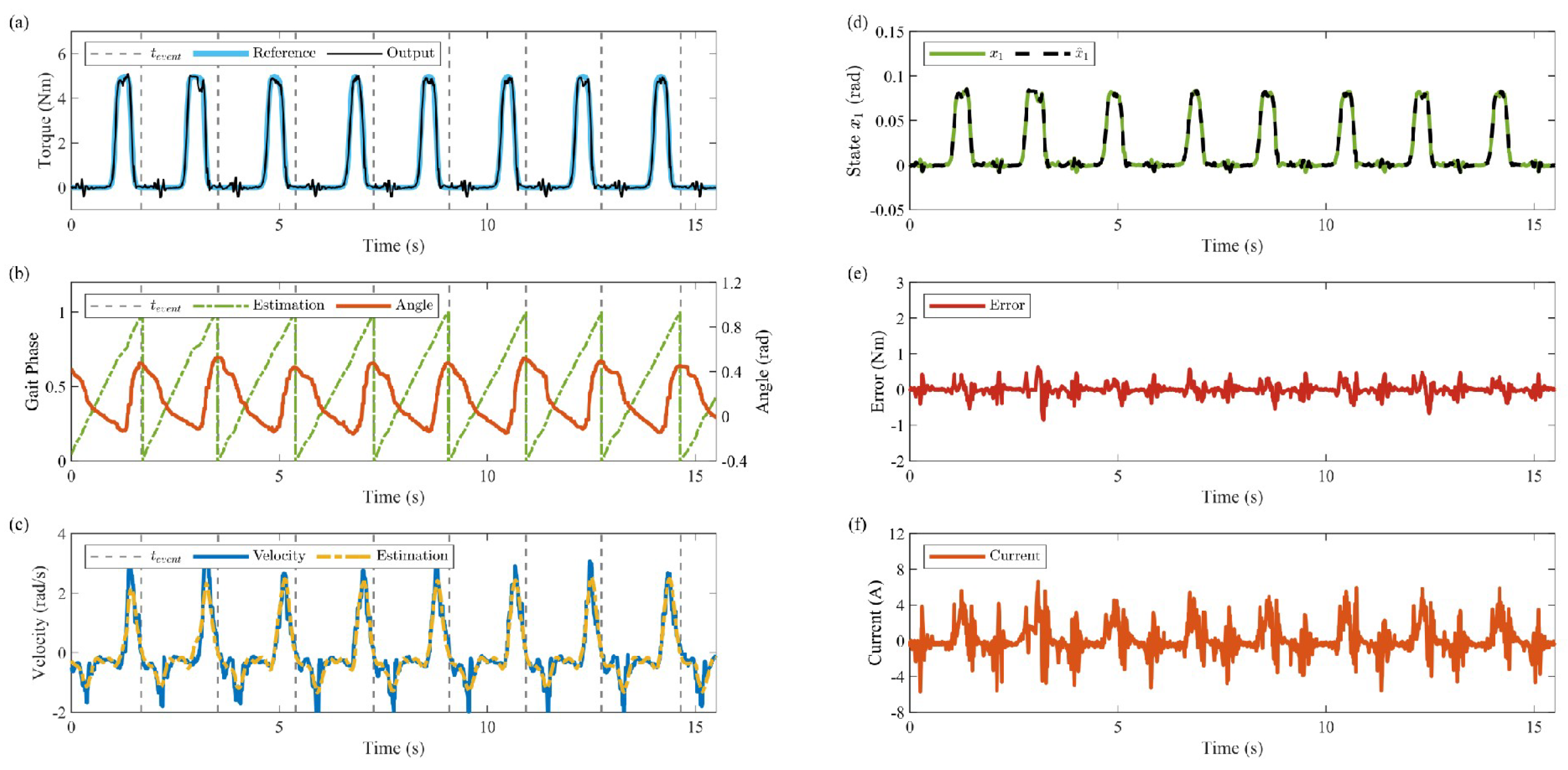
4.3. Results and Analysis

Figure 7 illustrates the cooperation between high-level and mid-level controllers to generate the reference assist torque. Figure 7a shows the angle-time curve of the user’s original gait. Figure 7b shows the derivative of the user’s original gait with respect to time, representing the angular velocity–time curve. The system’s estimate of angular velocity adapts to the true value over time. Figure 7c shows the phase output of the adaptive phase oscillator, which adapts to the user’s original gait and performs mismatch correction based on characteristic events. Figure 7d shows the reference assist torque output through the parametric single-peak curve. The overall tracking state is ideal and the output conforms to the gait curve, showing the effectiveness of the high-level controller and mid-level controller.

The simulation results for the CSMC+ESO method are presented in Figure 8. Figure 8a shows that the CSMC strategy achieves complete tracking of the ideal torque throughout the entire travel phase, with no significant overshoot or hysteresis. The tracking of ESO is demonstrated in Figure 8b,c,f, where ESO’s observations of the velocity and lumped disturbance are highly accurate, confirming that ESO increases the robustness of the system. The highly accurate estimation of disturbances ensures the system’s responsiveness to lumped disturbance. Figure 8d displays the actuator, demonstrating that the CSMC method used in this paper reduces the jitter issue found in traditional SMC, resulting in smoother curves. Figure 8e illustrates the tracking error for the CSMC strategy, with the absolute error value maintained within 0.6, confirming its high robustness and accuracy. The result demonstrates the effectiveness of the designed low-level control strategy.

Meanwhile, this study focuses on three statistical metrics of the three control algorithms—Average Tracking Error (ATE), Standard Deviation Error (SDE), and Maximum Absolute Error (MAE)—which are calculated by selecting the tracking error during 0 s ≤t≤ 25 s and are shown in the

Table 1. Indicators for each of the three control strategies.

Control Strategy	ATE	SDE	MAE
$CSMC+ESO$	0.0268	0.0484	0.5642
$ADRC$	0.0357	0.0544	0.6461
$PID$	0.0604	0.0953	0.5115

.

All three control strategies have been demonstrated to be capable of tracking the ideal trajectory under simulation. However, a clear discrepancy in tracking error is evident, as illustrated in Figure 9. The tracking error over time for each strategy is depicted in the above figure, where the CSMC algorithm exhibits the smallest error, followed by the ADRC algorithm. The PID algorithm demonstrates the most significant error, particularly in the presence of perturbations. In such cases, the CSMC algorithm remains stable, while the other two algorithms are affected to varying degrees.

The CSMC+ESO algorithm demonstrates superior performance in terms of ATE metrics when compared to the other two strategies. CSMC exhibits higher tracking accuracy. Furthermore, the superiority of CSMC+ESO in SDE metrics demonstrates that the low-level control strategy employed in this paper controls jitter vibration more effectively than the other two mainstream control strategies.The use of ESO enhances the ability of the present strategy to resist a wide range of disturbances, and the improvement of SMC is considered successful without much loss of robustness. It significantly outperforms the algorithms used for comparison in terms of MAE metrics, highlights the high robustness of the SMC-based strategy under external perturbations, and proves that the control strategy designed in this study possesses a faster convergence speed and shows improved transient performance.

4.4. Experimental Protocol

To evaluate the performance of the hip exoskeleton controller, treadmill-based experiments were conducted with five healthy male participants (age: 26 ± 2 y.o.; height: 175.3 ± 5.2 cm; weight: 68 ± 9.2 kg). All participants provided written informed consent prior to testing. The experimental setup is illustrated in Figure 10. Participants performed walking trials while wearing the exoskeleton under three distinct control approaches, including the novel control strategy proposed in this study along with conventional PID control and ADRC. Twenty trials were conducted for each control strategy (5 participants × 4 trials per participant), with each 5-minute trial followed by a 30-minute rest period to control for fatigue. For analysis, a representative 15-second interval comprising 8 complete gait cycles was selected from each trial. The treadmill maintained a constant speed of 1 m/s throughout all experiments.

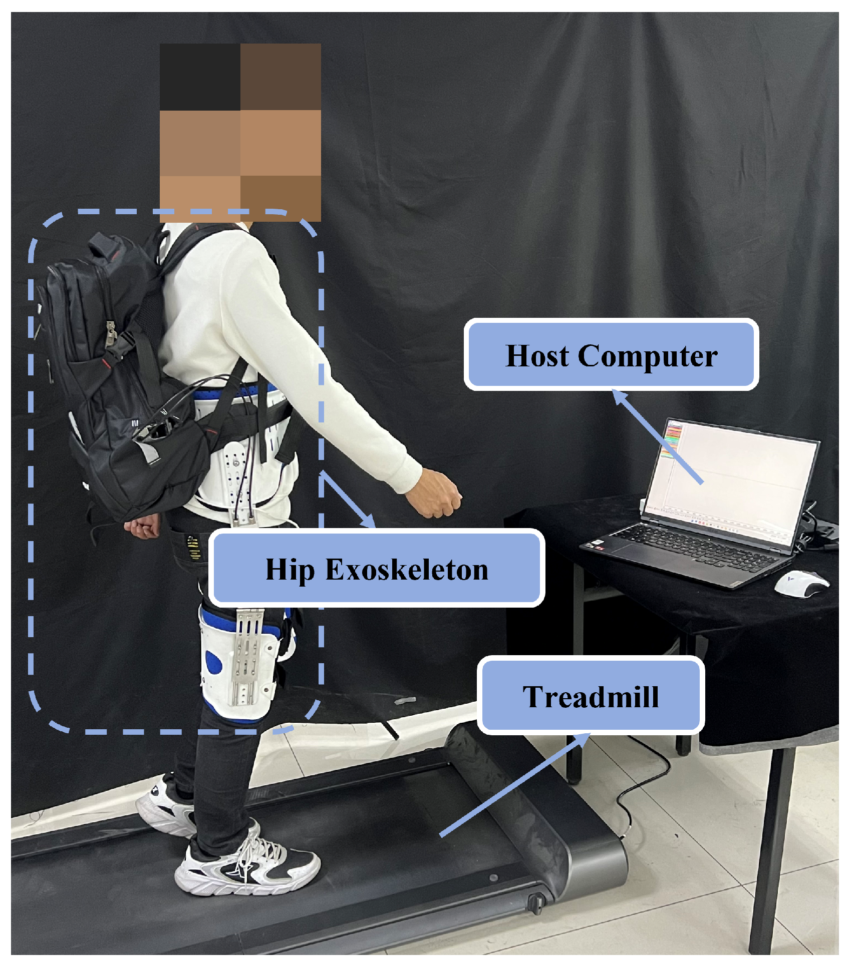
5. Preliminary Human Subject Experiments

5.1. Controllers for Comparison

This study conducts a comparative analysis of the proposed CSMC+ESO control strategy against both PID control and ADRC schemes. The parameters of these controllers are selected as follows:

(a) The parameters of the CSMC+ESO is given as follows: The gains for ESO are selected as ${\lambda }_1=3{\lambda }_0$, ${\lambda }_2=3{{\lambda }_0}^2$, and ${\lambda }_3={{\lambda }_0}^3$, where ${\lambda }_0=200$, and the CSMC parameters are selected as $c_1=22500,c_2=300$, and $\kappa =1\times {10}^5$. To ensure rigorous experimental comparison, the control parameters of ADRC are kept identical to those of CSMC+ESO.

(b) The structure of the PID is given as follows:

$$u=J_{m0}{K}^{-1}(k_p{e}_1+k_d{e}_2+k_i\underset{0}{\overset{t}{\int }}{e}_{1}dt)$$

(46)

The PID parameters are set to $k_p=22500,k_i=1\times {10}^5,k_d=300$. The parameters of adaptive phase oscillator are set to $\psi =6.5$, $\epsilon =0.7$, $K_{\phi }=5$. The Parameterized assistive torque curve are set to ${\phi }_{st}=0.55$, ${\phi }_{rs}=0.2$, $\gamma =6$.

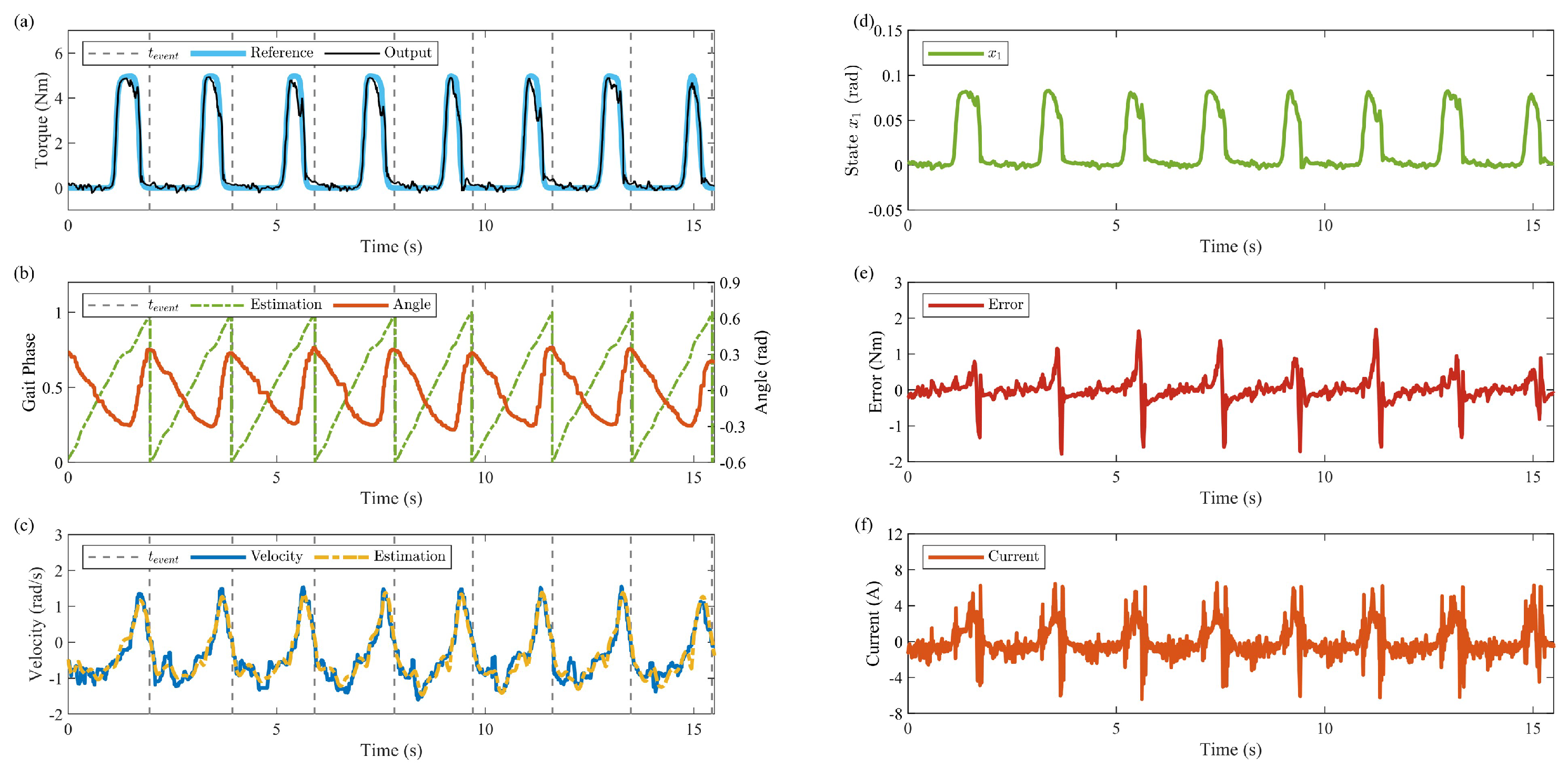
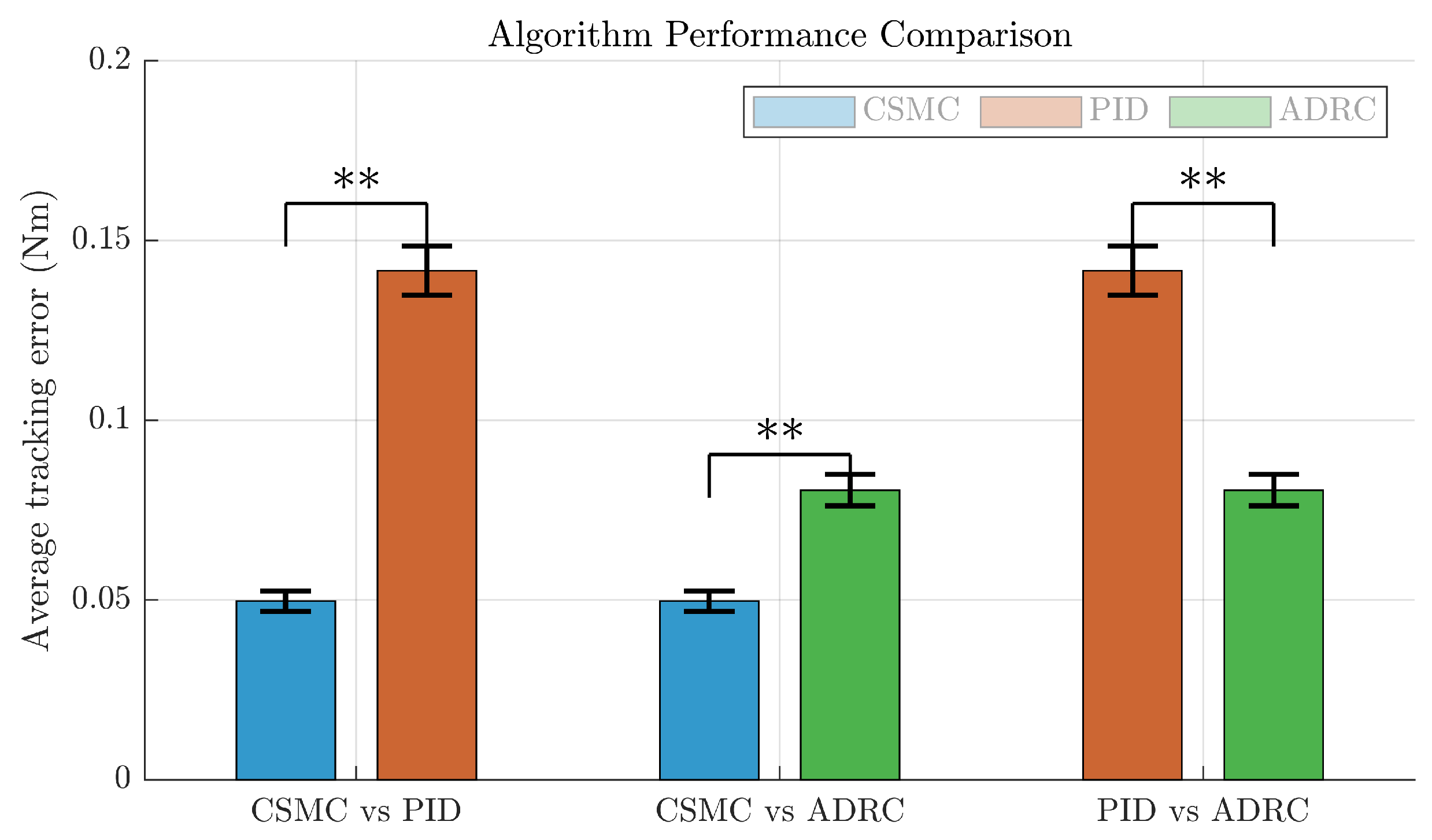
5.2. Results and Analysis

As shown in Figure 11, Figure 11a indicates that the output torque accurately tracks the reference torque during actual walking, demonstrating that the low-level controller performs as designed and aligns with the simulation results. Figure 11b illustrates the operation of the adaptive oscillator, which outputs a phase with good linearity and uses characteristic gait events for mismatch correction to match the gait phase. From the initial stage, it can be seen that, as the adaptive phase oscillator converges, the estimation of the gait phase by the adaptive phase oscillator gradually agrees with the actual gait phase, thus improving the tracking effect. Figure 11c presents the actual angular velocity and the controller’s estimated value, showing that the estimation is accurate and reliable for controller use. Figure 11d shows the deflection angle observed by the ESO for the SEA, which is precisely tracked and can be used to enhance system robustness. Figure 11e depicts the error during the experiment, which is maintained within a low range (lower than $1.05$). Figure 11f illustrates the motor control current of the system, which remains smooth and stable throughout the experiment, meeting the requirements for practical applications.

Figure 12 and Figure 13 present the experimental data of the exoskeleton under ADRC and PID strategies, respectively.

Table 2. Indicators for each of the two control strategies.

Control Strategy	ATE	SDE	MAE
$CSMC+ESO$	0.0501	0.0553	0.4735
$ADRC$	0.0956	0.1228	0.8468
$PID$	0.1502	0.2860	0.9496

lists three statistical indicators for the these control methods, where ATE, SDE, and MAE are calculated using tracking errors during 0 s $\le t\le$ 15 s. Figure 14 compares the average tracking accuracy of the three control methods, with each method evaluated on 20 independent datasets. Specifically, Figure 12a and Figure 13a demonstrate the output torque tracking performance relative to reference torque under ADRC and PID control, respectively. Figure 12b and Figure 13b illustrate the adaptive phase oscillator’s response to subject gait during ADRC and PID experiments. Figure 12c and Figure 13c compare the controller’s estimated angular velocity with the true values, showing the estimated values generally meet the requirements and closely fit the true values in both experiments. Figure 12d and Figure 13d display the deflection angle of the SEA during the ADRC and PID experiment, revealing jitter phenomena compared to the curve in Figure 11, which indicates that the CSMC+ESO control strategy designed in this study outperforms the ADRC and PID algorithms in terms of robustness. The overall tracking accuracy of PID is lower, confirming its limited robustness against uncertainties and external disturbances. In contrast, the high robustness of the proposed control strategy is verified by the MAE metric, consistent with the results shown in Figure 11, Figure 12 and Figure 13. Figure 12e and Figure 13e depict the tracking error of the ADRC and PID algorithms, showing that it is inferior to the proposed algorithm in terms of tracking accuracy, maximum error, and average error. Notice that the ATE metrics also indicate that the proposed control strategy in the experiment converges faster, proving that the CSMC+ESO control strategy indeed has higher accuracy. Table 2 can illustrates this more precisely. Figure 12f and Figure 13f show the motor input current during the ADRC and PID experiments, with larger extreme values, higher instantaneous rates of change, and more jitter compared to Figure 11. The conclusion is also shown in the SDE metric, which verifies that the proposed improvement reduces jitter vibration in the control process, making it less demanding on the controller and motor and more favorable for practical applications.

The effectiveness of the control strategy and mechanism improvements designed in this paper has been confirmed through simulation experiments on a treadmill. The graphical results and data demonstrate that the exoskeleton system can apply precise and comfortable assisting torque to the user. Additionally, the system is adaptive, capable of adjusting its phase in accordance with the user’s gait. Participants reported experiencing a clear and effective assisting torque during the walking process.

6. Conclusions

This paper proposed a real-time assistive torque controller based on sliding-mode control for an SEA-driven lower limb exoskeleton. A novel variable stiffness SEA consisting of two sets of elastic elements, with excellent cushioning properties and smooth torque output, was designed for the hip joint. A robust composite control strategy, combining an adaptive phase oscillator, a single-peak curve, and a low-level CSMC+ESO controller, was developed to enhance torque tracking performance under uncertainties. Experiments confirmed that the exoskeleton could provide precise and adaptive assisting torque, with participants reporting a clear and effective assistive experience.

References

1. Sheng, J.; Ding, R.; Yang, H. Corporate green innovation in an aging population: Evidence from Chinese listed companies. Technol. Forecast. Soc. Chang. 2024, 202, 123307. [Google Scholar] [CrossRef]
2. Krahn, G.L. WHO World Report on Disability: A review. Disabil. Health J. 2011, 4, 141–142. [Google Scholar] [CrossRef] [PubMed]
3. World Health Organization. The Global Burden of Disease: 2004 Update; World Health Organization: Geneva, Switzerland, 2008; Volume 14. [Google Scholar]
4. Sun, D.; Ma, J.; Ding, Y.; Luo, D. Human-exoskeleton oscillation model and qualitative analysis of interaction and functional practicality of exoskeletons. Appl. Math. Model. 2023, 120, 40–56. [Google Scholar] [CrossRef]
5. Ding, T.J.; Kang, C.C.; Han, W.; Ariannejad, M.; Kang, L.Y.; Ren, C.K. Development trend of robotic exoskeletons. In Proceedings of the 2023 IEEE International Conference on Cybernetics and Intelligent Systems (CIS) and IEEE Conference on Robotics, Automation and Mechatronics (RAM), Penang, Malaysia, 9–12 June 2023; pp. 114–121. [Google Scholar]
6. Qiu, S.; Pei, Z.; Wang, C.; Tang, Z. Systematic review on wearable lower extremity robotic exoskeletons for assisted locomotion. J. Bionic Eng. 2023, 20, 436–469. [Google Scholar] [CrossRef]
7. Hasan, S.K.; Dhingra, A.K. State of the art technologies for exoskeleton human lower extremity rehabilitation robots. J. Mechatron. Robot. 2020, 4, 211–235. [Google Scholar] [CrossRef]
8. Shin, Y.J.; Kim, G.T.; Kim, Y. Optimal design of multi-linked knee joint for lower limb wearable robot. Int. J. Precis. Eng. Manuf. 2023, 24, 967–976. [Google Scholar] [CrossRef]
9. Qian, Y.; Han, S.; Wang, Y.; Yu, H.; Fu, C. Toward improving actuation transparency and safety of a hip exoskeleton with a novel nonlinear series elastic actuator. IEEE/ASME Trans. Mechatron. 2022, 28, 417–428. [Google Scholar] [CrossRef]
10. Lee, Y.; Kim, Y.J.; Lee, J.; Lee, M.; Choi, B.; Kim, J.; Park, Y.J.; Choi, J. Biomechanical design of a novel flexible exoskeleton for lower extremities. IEEE/ASME Trans. Mechatron. 2017, 22, 2058–2069. [Google Scholar] [CrossRef]
11. Zhou, L.; Chen, W.; Wang, J.; Bai, S.; Yu, H.; Zhang, Y. A novel precision measuring parallel mechanism for the closed-loop control of a biologically inspired lower limb exoskeleton. IEEE/ASME Trans. Mechatron. 2018, 23, 2693–2703. [Google Scholar] [CrossRef]
12. Xi, R.; Zhu, Z.; Du, F.; Yang, M.; Wang, X.; Wu, Q. Design concept of the quasi-passive energy-efficient power-assisted lower-limb exoskeleton based on the theory of passive dynamic walking. In Proceedings of the 2016 23rd International Conference on Mechatronics and Machine Vision in Practice (M2VIP), Nanjing, China, 28–30 November 2016; pp. 1–5. [Google Scholar]
13. Gams, A.; Petrič, T.; Debevec, T.; Babič, J. Effects of robotic knee exoskeleton on human energy expenditure. IEEE Trans. Biomed. Eng. 2013, 60, 1636–1644. [Google Scholar] [CrossRef]
14. Arazpour, M.; Chitsazan, A.; Bani, M.A.; Rouhi, G.; Ghomshe, F.T.; Hutchins, S.W. The effect of a knee ankle foot orthosis incorporating an active knee mechanism on gait of a person with poliomyelitis. Prosthet. Orthot. Int. 2013, 37, 411–414. [Google Scholar] [CrossRef] [PubMed]
15. Jin, X.; Cui, X.; Agrawal, S.K. Design of a cable-driven active leg exoskeleton (C-ALEX) and gait training experiments with human subjects. In Proceedings of the 2015 IEEE International Conference on Robotics and Automation (ICRA), Seattle, WA, USA, 26–30 May 2015; pp. 5578–5583. [Google Scholar]
16. Ortiz, J.; Di Natali, C.; Caldwell, D.G. XoSoft-iterative design of a modular soft lower limb exoskeleton. In Proceedings of the International Symposium on Wearable Robotics, Pisa, Italy, 16–20 October 2018; Springer: Cham, Switzerland, 2018; pp. 351–355. [Google Scholar]
17. Dingan, S.; Hua, J.; Lia, Y. Research on Assisting Control and Oxygen Metabolism Testing of Rope Driven Flexible Exoskeleton. Mater. Sci. Eng. Appl. 2023, 40, 517–525. [Google Scholar]
18. Xu, D.; Liu, X.; Wang, Q. Knee exoskeleton assistive torque control based on real-time gait event detection. IEEE Trans. Med Robot. Bionics 2019, 1, 158–168. [Google Scholar] [CrossRef]
19. Li, C.; He, Y.; Chen, T.; Chen, X.; Tian, S. Real-time gait event detection for a lower extremity exoskeleton robot by infrared distance sensors. IEEE Sens. J. 2021, 21, 27116–27123. [Google Scholar] [CrossRef]
20. Huang, B.; Chen, M.; Shi, X.; Xu, Y. Gait event detection with intelligent shoes. In Proceedings of the 2007 International Conference on Information Acquisition, Seogwipo, Republic of Korea, 8–11 July 2007; pp. 579–584. [Google Scholar]
21. Zhang, J.; Fiers, P.; Witte, K.A.; Jackson, R.W.; Poggensee, K.L.; Atkeson, C.G.; Collins, S.H. Human-in-the-loop optimization of exoskeleton assistance during walking. Science 2017, 356, 1280–1284. [Google Scholar] [CrossRef]
22. Wen, Y.; Si, J.; Brandt, A.; Gao, X.; Huang, H.H. Online reinforcement learning control for the personalization of a robotic knee prosthesis. IEEE Trans. Cybern. 2019, 50, 2346–2356. [Google Scholar] [CrossRef]
23. Li, M.; Wen, Y.; Gao, X.; Si, J.; Huang, H. Toward expedited impedance tuning of a robotic prosthesis for personalized gait assistance by reinforcement learning control. IEEE Trans. Robot. 2021, 38, 407–420. [Google Scholar] [CrossRef]
24. Yang, X.; Fu, Z.; Yi, S.; Qi, B.; Guo, Z. Adaptive Oscillator-Based Gait Event Detection and Trajectory Planning for Lower Limb Exoskeleton. In Proceedings of the 2024 World Rehabilitation Robot Convention (WRRC), Shanghai, China, 23–26 August 2024; pp. 1–6. [Google Scholar]
25. Xue, T.; Wang, Z.; Zhang, T.; Zhang, M. Adaptive oscillator-based robust control for flexible hip assistive exoskeleton. IEEE Robot. Autom. Lett. 2019, 4, 3318–3323. [Google Scholar] [CrossRef]
26. Qian, Y.; Yu, H.; Fu, C. Adaptive oscillator-based assistive torque control for gait asymmetry correction with a nSEA-driven hip exoskeleton. IEEE Trans. Neural Syst. Rehabil. Eng. 2022, 30, 2906–2915. [Google Scholar] [CrossRef]
27. Zhang, T.; Li, Y.; Ning, C.; Zeng, B. Development and adaptive assistance control of the robotic hip exoskeleton to improve gait symmetry and restore normal gait. IEEE Trans. Autom. Sci. Eng. 2022, 21, 799–809. [Google Scholar] [CrossRef]
28. Suzuki, K.; Mito, G.; Kawamoto, H.; Hasegawa, Y.; Sankai, Y. Intention-based walking support for paraplegia patients with Robot Suit HAL. Adv. Robot. 2007, 21, 1441–1469. [Google Scholar] [CrossRef]
29. Farris, R.J.; Quintero, H.A.; Goldfarb, M. Preliminary evaluation of a powered lower limb orthosis to aid walking in paraplegic individuals. IEEE Trans. Neural Syst. Rehabil. Eng. 2011, 19, 652–659. [Google Scholar] [CrossRef] [PubMed]
30. Zhang, Y.; Cao, G.; Li, L.; Diao, D. AEKF-based trajectory-error compensation of knee exoskeleton for human–exoskeleton interaction control. Robot. Intell. Autom. 2024, 44, 84–95. [Google Scholar] [CrossRef]
31. Chen, Y.; Liang, L.; Wu, M.; Wang, Y.; Liu, C. Experimental verification study on trajectory tracking of a novel rehabilitation exoskeleton shoulder joint. J. Mech. Med. Biol. 2019, 19, 1940037. [Google Scholar] [CrossRef]
32. Khan, R.F.A.; Rsetam, K.; Cao, Z.; Man, Z. Singular perturbation-based adaptive integral sliding mode control for flexible joint robots. IEEE Trans. Ind. Electron. 2022, 70, 10516–10525. [Google Scholar] [CrossRef]
33. Pan, Y.; Li, X.; Wang, H.; Yu, H. Continuous sliding mode control of compliant robot arms: A singularly perturbed approach. Mechatronics 2018, 52, 127–134. [Google Scholar] [CrossRef]
34. Korayem, M.; Nekoo, S.R.; Kazemi, S. Finite-time feedback linearization (FTFL) controller considering optimal gains on mobile mechanical manipulators. J. Intell. Robot. Syst. 2019, 94, 727–744. [Google Scholar] [CrossRef]
35. Abdul-Adheem, W.R.; Ibraheem, I.K.; Humaidi, A.J.; Azar, A.T. Model-free active input–output feedback linearization of a single-link flexible joint manipulator: An improved active disturbance rejection control approach. Meas. Control 2021, 54, 856–871. [Google Scholar] [CrossRef]
36. Cheng, X.; Zhang, Y.; Liu, H.; Wollherr, D.; Buss, M. Adaptive neural backstepping control for flexible-joint robot manipulator with bounded torque inputs. Neurocomputing 2021, 458, 70–86. [Google Scholar] [CrossRef]
37. Chang, W.; Li, Y.; Tong, S. Adaptive fuzzy backstepping tracking control for flexible robotic manipulator. IEEE/CAA J. Autom. Sin. 2018, 8, 1923–1930. [Google Scholar] [CrossRef]
38. Gao, H.; He, W.; Zhou, C.; Sun, C. Neural network control of a two-link flexible robotic manipulator using assumed mode method. IEEE Trans. Ind. Inform. 2018, 15, 755–765. [Google Scholar] [CrossRef]
39. Diao, S.; Sun, W.; Su, S.F.; Zhao, X.; Xu, N. Novel adaptive control for flexible-joint robots with unknown measurement sensitivity. IEEE Trans. Autom. Sci. Eng. 2023, 21, 1445–1456. [Google Scholar] [CrossRef]
40. Tafrishi, S.A.; Hirata, Y. SPIRO: A Compliant Spiral Spring–Damper Joint Actuator With Energy-Based Sliding-Mode Controller. IEEE/ASME Trans. Mechatron. 2024, 29, 947–959. [Google Scholar] [CrossRef]
41. Suryawanshi, P.V.; Shendge, P.D.; Phadke, S.B. A boundary layer sliding mode control design for chatter reduction using uncertainty and disturbance estimator. Int. J. Dyn. Control 2016, 4, 456–465. [Google Scholar] [CrossRef]
42. Lu, B.; Fang, Y.; Sun, N. Continuous sliding mode control strategy for a class of nonlinear underactuated systems. IEEE Trans. Autom. Control 2018, 63, 3471–3478. [Google Scholar] [CrossRef]
43. Ginoya, D.; Shendge, P.; Phadke, S. Sliding mode control for mismatched uncertain systems using an extended disturbance observer. IEEE Trans. Ind. Electron. 2013, 61, 1983–1992. [Google Scholar] [CrossRef]
44. Wang, H.; Zhang, Z.; Tang, X.; Zhao, Z.; Yan, Y. Continuous output feedback sliding mode control for underactuated flexible-joint robot. J. Frankl. Inst. 2022, 359, 7847–7865. [Google Scholar] [CrossRef]
45. Zaare, S.; Soltanpour, M.R. Continuous fuzzy nonsingular terminal sliding mode control of flexible joints robot manipulators based on nonlinear finite time observer in the presence of matched and mismatched uncertainties. J. Frankl. Inst. 2020, 357, 6539–6570. [Google Scholar] [CrossRef]
46. Qian, Y.; Wang, Y.; Chen, C.; Xiong, J.; Leng, Y.; Yu, H.; Fu, C. Predictive locomotion mode recognition and accurate gait phase estimation for hip exoskeleton on various terrains. IEEE Robot. Autom. Lett. 2022, 7, 6439–6446. [Google Scholar] [CrossRef]
47. Qian, Y.; Chen, C.; Xiong, J.; Wang, Y.; Leng, Y.; Yu, H.; Fu, C. Terrain-Adaptive Exoskeleton Control With Predictive Gait Mode Recognition: A Pilot Study During Level Walking and Stair Ascent. IEEE Trans. Med. Robot. Bionics 2024, 6, 281–291. [Google Scholar] [CrossRef]
48. Chen, C.; Du, Z.; Zhang, H.; Dong, W. Double-mode switching control of a lower limb exoskeleton based on flexible drive joint. Jiqiren/Robot 2021, 43, 513–525. [Google Scholar]
Figure 1. Schematic of the mechanical design of the proposed SEA.
Actuators 14 00239 g001
Figure 2. Schematic diagram of the structure of a rotary series elastic element.
Actuators 14 00239 g002
Figure 3. Stiffness characteristic curve.
Actuators 14 00239 g003
Figure 4. The block diagram of the exoskeleton system.
Actuators 14 00239 g004
Figure 5. Architecture of the terrain-adaptive exoskeleton control.
Actuators 14 00239 g005
Figure 6. The schema of the parametric single-peak curve.
Actuators 14 00239 g006
Figure 7. The working process of adaptive phase oscillator.
Actuators 14 00239 g007
Figure 8. Simulation results of the CSMC+ESO control strategy.
Actuators 14 00239 g008
Figure 9. Simulation results of the three control strategies. (a1) Output response using the CSMC algorithm. (a2) Tracking error using the CSMC algorithm. (b1) Output response using the ADRC algorithm. (b2) Tracking error using the ADRC algorithm. (c1) Output response using the PID algorithm. (c2) Tracking error using the PID algorithm.
Actuators 14 00239 g009
Figure 10. The test platform of exoskeleton system.
Actuators 14 00239 g010
Figure 11. Experimental results based on the CSMC+ESO control strategy.
Actuators 14 00239 g011
Figure 12. Experimental results based on the ADRC strategy.
Actuators 14 00239 g012
Figure 13. Experimental results based on the PID control strategy.
Actuators 14 00239 g013
Figure 14. Comparison of average tracking errors across the three control algorithms. Error bars represent ± 1 SEM, and ** indicate statistically significant difference (p < 0.05).
Actuators 14 00239 g014