Article

Composite Adaptive Control of Robot Manipulators with Friction as Additive Disturbance

by
Daniel Gamez-Herrera
,
Juan Sifuentes-Mijares
,
Victor Santibañez
* and
Isaac Gandarilla
Instituto Tecnológico de La Laguna, Tecnológico Nacional de México, Blvd. Revolución y Av. Instituto Tecnológico de La Laguna S/N, Torreón C.P. 27000, Coahuila, Mexico
*
Author to whom correspondence should be addressed.
Actuators 2025, 14(5), 237; https://doi.org/10.3390/act14050237
Submission received: 21 March 2025 / Revised: 23 April 2025 / Accepted: 6 May 2025 / Published: 8 May 2025
(This article belongs to the Special Issue Nonlinear Control of Mechanical and Robotic Systems)

Abstract

:
In this paper, an adaptive control scheme composed of an estimated feed-forward compensation and a PD control law with three mutually independent estimators is proposed for the tracking of desired trajectories in joint space for a robotic arm. One of the estimators is used to identify inertial and geometrical parameters, while the others determine the two principal components of the friction phenomenon: the part whose magnitude is position-dependent but velocity-independent and the part whose magnitude is proportional to velocity. Next, the persistently exciting condition is satisfied for each regression matrix of the estimators in a way that is easier to prove than the classical structure. Then, uniform global asymptotic stability can be concluded for the tracking error, regardless of parametric convergence, by applying the direct Lyapunov theorem. This scheme has been applied experimentally for a robotic arm to verify the theoretical results. The experimental results yielded a better performance in both estimating the parameters and tracking, with a much simpler overall analysis than the alternatives consulted.

1. Introduction

Most applications of robot manipulators require at least partial knowledge of the relation of input variables to output variables. When such a relation is determined analytically, it is established in a set of ordinary differential equations. Such a set is called the dynamic model, and its behavior is characterized by the parameters it includes. Non-linear model-based control techniques require full knowledge of these parameters to design a controller. Computed torque is one of the main techniques used to undertake the tracking of desired trajectories in joint space for robot manipulators as it allows for feedback linearization, which consists of a form of transformation that leads to some linear closed-loop dynamics, which are not necessarily stable but are controllable [1]. However, it presents a significant drawback, namely, that all the parameters in the dynamic model must be known, which is not the case; at the modeling stage, only the structure of the dynamic model can be assumed to be known exactly.
A complementary approach in these cases is the so-called adaptive control theory, whose methodologies involve the field of system identification; this theory considers a set of differential equations as a grey box model, assuming its structure a priori knowledge and then estimating the model parameters [2]. Subsequent to the modeling stage is the parametric identification stage wherein the linear parametrization of robot dynamics is often used, and an identification algorithm is implemented to estimate the unknown parameters [3]. This approach is not only useful in a situation where the constant parameters are not known a priori, but they can vary as the robot dynamics evolves [4]. This implies that at least one parameter may be time-variant and that if the controller is not continuously redesigned, it may not properly control the changing plant.
The last case is the most realistic proposal as even gravitational interaction is not constant; it is a distributed parameter over spacetime. A nominal mid-range value on Earth is defined as it is greater at the poles than at the Equator [5]; however, variation in its magnitude can be neglected as it is small. On the other had, the phenomenon of friction cannot be neglected as its contribution can affect the dynamic behavior of a mechanical system such as a robot manipulator [6]; even in theory, it may change the stability conclusions because of its dissipative effect. Extensive research concerning the friction phenomenon has been carried out since the work of Coulomb and Amontons, who established some dependencies of the coefficient of friction on conditions such as the normal force, the size of the contact area, the sliding velocity, and atmospheric variables [7].
The need for a friction model that takes into account the fact that the friction force at zero velocity is higher than the friction in motion, and that the decrease from static to kinetic friction is a continuous process, led to some more complex models such as the Armstrong–Hélouvry model [8]. This model incorporates the Stribeck effect, which describes the decrease in friction force with an increase in velocity close to null velocity as a non-linear function of velocity, i.e., as a transition between the maximum static friction and the typical Coulomb friction, and as a viscous friction, i.e., a regime proportional to the velocity. A conceptual representation is depicted in Figure 1.
Despite the successful application of this kind of static model, it is indisputable that friction as a phenomenon possesses its own dynamics. Some time later, dynamic friction models appeared, such as the Dahl model [9], and a generalization of it, the LuGre model [10], with the former being a one-state variable model whose behavior is similar to that of a non-linear spring in the elastoplastic domain. For small deflections, this is governed by Hooke’s law and is approximately linear, but for large deflections, non-reversible changes appear, which reveals a frictional lag between velocity reversals. Its importance lies in the discovery of the existence of a hysteresis between the necessary force before the sliding occurs and the related displacement [11]. The latter is an extension of Dahl model. The LuGre model introduces a velocity-dependent exponential function instead of a constant inside the dynamics of the internal state; since the steady state of the Dahl model is equivalent to the Coulomb friction, it does not take into account the Stribeck effect [12]. This strategy is not only useful in considering the Stribeck effect; it is fundamental when it comes to handling anisotropy, i.e., the fact that friction force is not uniform in all directions. The LuGre model has been extensively used for friction compensation in control applications because of two key factors: that the model state possesses a simple physical interpretation as the average deflection of a bristle, and its continuous first-order bounded dynamics [13]. Nonetheless, the experimental parameters introduced in this model, the fact that the model’s internal states are not measurable, and its time-varying nature suggest that much more a priori knowledge is required [14].
Other main alternative approach based on control theory is to compensate any deviation from the nominal dynamics with some control strategy using the data acquired from sensors. Representative approaches, such as neuronal networks [15], fuzzy logic [16], fault tolerant schemes [17], and Bayesian optimization [18], have been researched throughout this past decade, but they have been found to be too complex in structure, to be computationally inefficient, and to involve more sensors, and their stability has also proven hard to prove. A control scheme that overcomes the drawbacks identified in recent research is proposed in the present work.

Contributions

In this work, a technical proposal for estimating friction coefficients online is presented, using a key modularity feature in the design of the controller. The regression matrix of the identifier achieves some useful boundedness properties independently of the controller. The proposed scheme possesses the following novelties and advantages:
  • A decomposition of the robot manipulator model into an adequate linear parametrization for the conservative part and another for the non-conservative part is presented.
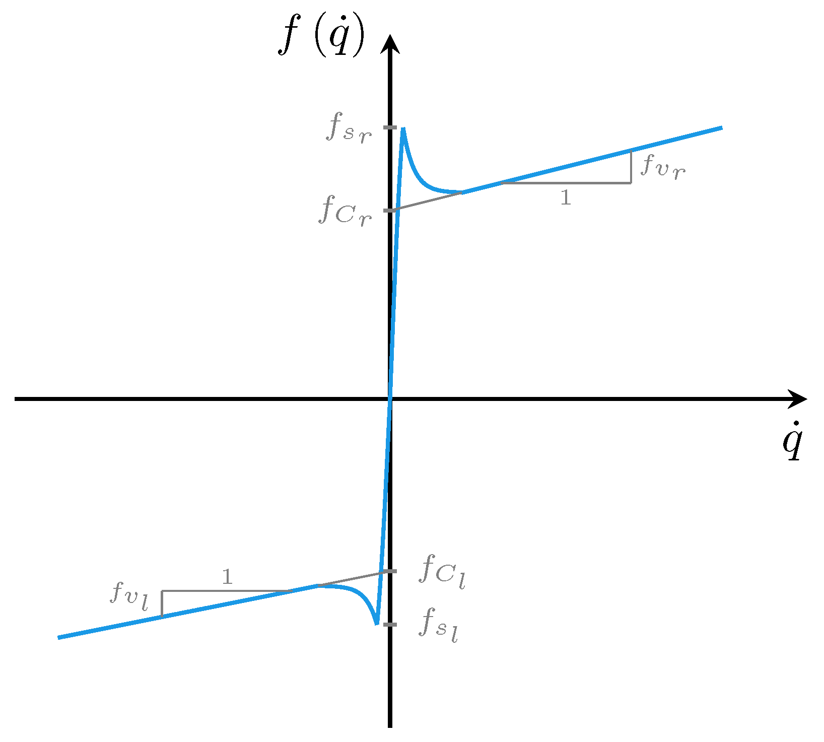
  • The friction phenomenon is characterized as two independent additive disturbances that can be linearly parametrized in terms of the physical coefficients of friction with a quiet simple regression matrix.
  • A separation into three simpler regression matrices is performed, which allows us to deal with them one by one and to find the upper and lower bounds that satisfy the persistent excitation condition for each of them.
  • A relaxation in the persistent excitation condition is made for the overall regression matrix that arises when the well-known swapping technique is applied. Both concepts are presented in detail in Section 3.3.
  • Lyapunov analysis is developed to support the fact that the robust control methodology in the designing stage of the controller is compensating for the disturbances while guaranteeing that the tracking position and velocity errors converge asymptotically to zero.
  • An effective practical compensation for friction, not involving a cumbersome dynamic model of friction and staying as simple as possible in stability analysis within a passivity framework, is presented, performing the tracking of the desired trajectories in joint space successfully.

2. Problem Formulation

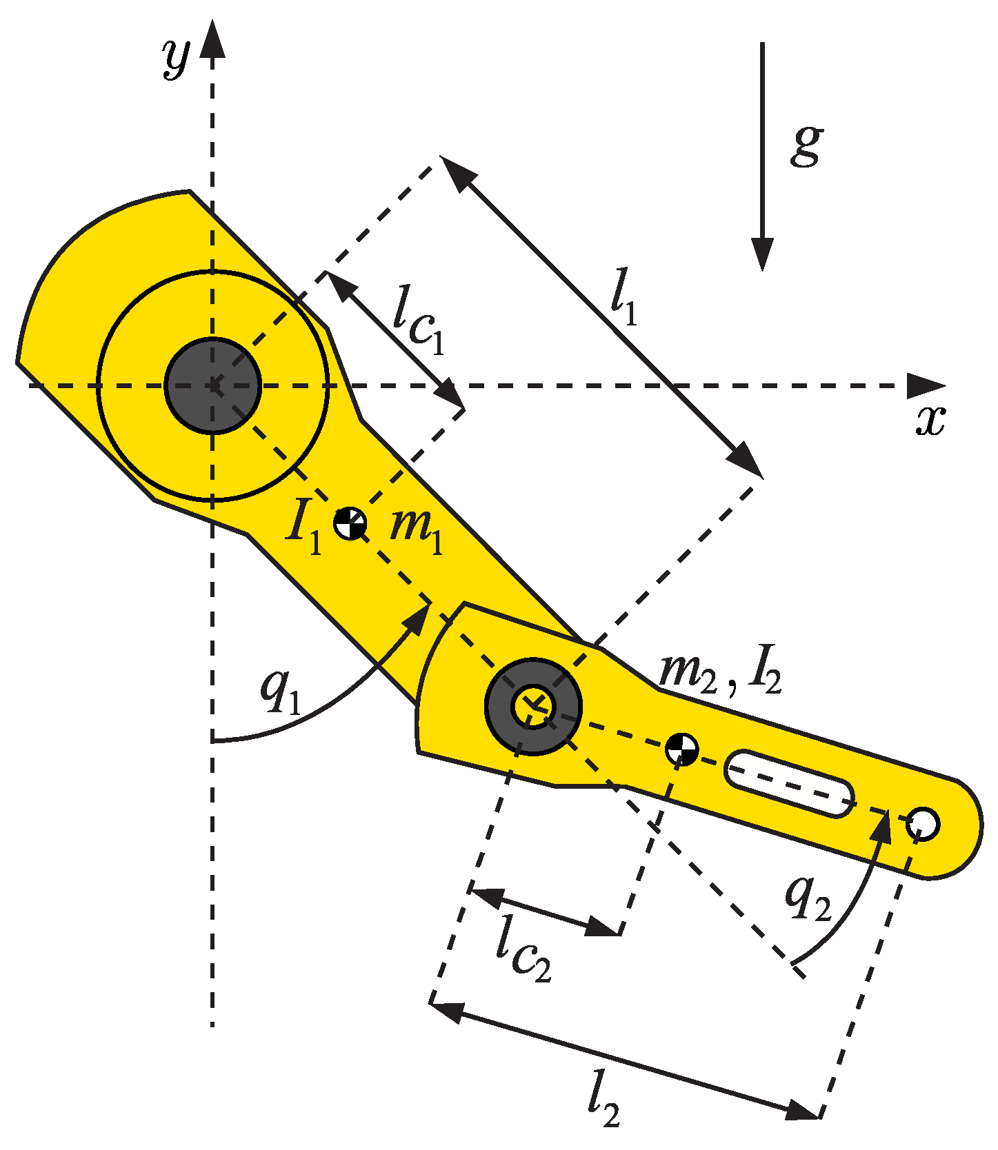
2.1. Robot Manipulator Model

The dynamic model in the joint-space of a general n-degrees-of-freedom robot manipulator with rigid links considering friction in the joints can be written in the compact vectorial form [19,20]:
M q q ¨ + C q , q ˙ q ˙ + g q + f q ˙ , t = τ ,
where the joint positions, velocities, and acceleration vectors are indicated as q , q ˙ , q ¨ R n × 1 , respectively. M R n × n denotes the inertia matrix, and C R n × n denotes a centripetal-Coriolis matrix. The vector of generalized forces due to gravity is represented as g R n × 1 , the vector of non-conservative forces due to friction is designated as f R n × 1 , and τ R n × 1 denotes the vector of exogenous torques.
In regards to the vector of non-conservative forces due to friction, a time-variant model is taken into account to describe two major contribution components of this phenomenon with non-lumped elements, exhibiting regimes of transition. These include the one that considers the anisotropy of the Coulomb-like friction coefficients and the one that considers the transition threshold due to the non-linearity close to zero velocity in the viscous-like friction coefficients. Thus, the model of f is composed as follows:
f q ˙ , t = F C t tanh k q ˙ + F v t q ˙ ,
where F C t R n × n is a diagonal matrix whose elements are the coefficients of the Coulomb-like friction, the first term of (2), and F v t R n × n is a diagonal matrix whose elements are the coefficients of the viscous-like friction, the second term of (2). On the other hand, the hyperbolic tangent function in its vectorial form is denoted as tanh k q ˙ R n × 1 , with k > 0 , and it is used as a regularization of the typical discontinuous sign function, i.e., as a continuous relation dependent of the joint velocity [21]. Furthermore, the election of time-varying coefficients at the Coulomb-like friction term aims to describe the change in the magnitude of the non-conservative force contribution when the joint changes its direction of rotation; i.e., friction exhibits an anisotropic behavior since its effects do not have the same magnitude in all directions. Moreover, the use of time-varying coefficients at the viscous-like friction term is a technical proposal introduced to facilitate the transition from the static regime to the dynamic regimen.

2.2. Properties of the Dynamic Model

All the dynamics of the specific kind of robotic manipulator previously described have been captured in model (1), i.e., when no other unmodeled dynamic or perturbation is involved in the plant. Some fundamental properties of the dynamic model for this manipulator are presented in this section for its use in the control design stage. All of the properties and their proofs can be consulted in [19,20,22].
Property 1. 
The dependence of the conservative part of the manipulator model on the dynamic parameters of each of its individual terms is linearly parametrizable in terms of a new set of unknown parameters θ * R p × 1 in the form
M q , θ * q ¨ + C q , q ˙ , θ * q ˙ + g q , θ * = Y q , q ˙ , q ¨ θ * ,
where Y q , q ˙ , q ¨ R n × p is the regressor matrix, which is only dependent on the trajectories.
Property 2. 
The centripetal Coriolis matrix C q , q ˙ is related to the inertia matrix M q by the identity
q T M ˙ q 2 C q , q ˙ q = 0 , q , q ˙ R n × 1
since the matrix M ˙ q 2 C q , q ˙ is skew-symmetric.
Property 3. 
The inertia matrix M = M T R n × n is a symmetric, uniformly positive definite M q > 0 for all q and uniformly bounded above and below by
μ 1 I M q μ 2 I < , μ 1 , μ 2 > 0 , I R n × n .
Furthermore, in order to exploit the dissipative characteristic of friction, the vector f q ˙ , t in (2) will be treated as an additive disturbance. First, a convenient linear reparametrization in friction coefficients is presented:
f q ˙ , t = diag tanh k q ˙ diag F C t + diag q ˙ diag F v t ,
where, for the present work, the diagonal operator takes a matrix of n × n and returns a n × 1 vector, whose elements are the matrix diagonal elements; alternatively, it takes a n × 1 vector and returns a diagonal matrix of n × n , whose elements are the elements of the vector.
Property 4. 
For a robot manipulator with anisotropic friction and continuous transition regimens around zero velocity in its joints, a reparametrization in terms of the friction coefficient can be express as
f q ˙ , t = Y C q ˙ θ C t + Y v q ˙ θ v t ,
where Y C q ˙ R n × n is the regressor matrix associated with the time-varying Coulomb-like friction coefficients θ C t R n × 1 . Similarly, Y v q ˙ R n × n is the regressor matrix associated with the time-varying viscous-like friction coefficients θ v t R n × 1 .

2.3. Control Objective and Identification Objective

Consider the robot model (1): the control objective is that the joint positions of the robot q track the desired position trajectories q d t asymptotically, i.e.,
lim t q d t q t = 0 R n ,
for all initial configurations q 0 , q d 0 , where q d t is an arbitrarily chosen continuous function and at least once differentiable. Moreover, it is supposed that q d t and q ˙ d t are known bounded vector functions, but the inertial and geometric parameter vector θ * , the Coulomb-like friction coefficients vector θ C t , and the viscous-like friction coefficients vector θ v t are not exactly known. Thus, the identification objective is that the estimation of the parameter vectors θ t , θ ^ C t , and θ ^ v t track the nominal parameter vectors θ * , θ C t , and θ v t asymptotically:
lim t θ * θ t = 0 R p × 1 , lim t θ C t θ ^ C t = 0 R n × 1 , lim t θ v t θ ^ v t = 0 R n × 1 .

2.4. Motivation of the Proposed Scheme

Considering the major drawbacks of existing dynamic friction models, a more practical scheme is desired for robotics applications, i.e., one that does not require the further empirical investigation of any other interdisciplinary fields, such as tribology, materials science, or solid mechanics, but one that is entirely based in control theory and the properties of the robot manipulator as a mechanical system. Inspired by the fact that the friction phenomenon must be characterized by a dissipative behavior, as well as previous results [23,24], the passivity framework seems reasonable to explore. As an alternative to the model-based methods used to describe friction, a straightforward method for friction compensation can be implemented by assuming the basic structure of the friction phenomenon, introducing time-varying coefficients to estimate the amplitude and timing of the contribution of each of the two major components of friction and determining an identification algorithm that satisfies this purpose using adaptive control theory.
This approach of treating friction allows us to parameterize the dynamic model in a novel way, and, combined with the passivity framework, it allows us to deal with the non-conservative part of the dynamics in the stability analysis and the identification algorithm analysis to guarantee the control objective and parametric convergence. For the former, it allows us to propose simple quadratic Lyapunov functions for each estimator and then only to add them, making the analysis as simple as it can be. For the latter, it simplifies the process of finding the bounds of the regressor matrix of each estimator and the proof that they satisfy the persistent excitation condition. All of this leads to a complete estimated feed-forward compensation that, along with an in-disguise PD controller using a sliding mode variable s , is sufficient to prove, to the best of the authors’ knowledge, the control objective and the identification objective previously stated in the easiest way, demonstrating quite-good experimental performance with a two-degree-of-freedom robotic arm.
The main benefits from the choice of the sliding mode control approach are the following:
  • It makes the control objective straightforward to conclude since the variable s conveys enough information of q and q ˙ in order to show that its boundedness and convergence to zero imply those of q ˜ and q ˜ ˙ .
  • It removes the computational complexity from the computed torque as the inverse inertia matrix does not have to be determined.
  • Since it is a robust control method, and since the two major components of friction are considered as disturbances, it rejects the small changes in the disturbances, i.e., the transition between static and dynamic regimes.
The latter phenomenon is always present in most applications with an inherently digital controller as the physical realization of the controller is established in a discrete time domain via two processes: amplitude discretization, referred to as quantization, and time discretization, referred to as sampling [25]. This induces (frequently underestimated) non-linear unmodeled dynamics, ubiquitous in the triggering of all actuators, since every time the actuator is activated, there is small interval of time at which the friction force transitions between a quasistatic state, in which movement is set to stand-by, and a motion state after overcoming a threshold to break the equilibrium of internal conservative forces, i.e., a state where the elastic deformation between the surfaces is present without sliding.

3. Preliminaries

3.1. Lyapunov Stability

Some basic concepts to prove the uniform global asymptotic stability of a dynamic system are presented next [22]. Consider a general dynamical system described by
x ˙ t = f t , x t , x 0 R n , t 0 ,
where the vector x t R n refers to the state of the dynamical system in (8), and x 0 R n is called the initial condition. A constant vector x e R n is an equilibrium or equilibrium state of the system (8) if
f t , x e = 0 t 0 .
A function V : R + × R n R + is a Lyapunov function for the equilibrium x = 0 of the equation (8) if the following apply:
  • V t , 0 = 0 , t 0
  • V t , x > 0 , x 0 R n , t 0
  • Its partial derivatives are continuous.
  • Its total time derivative along the trajectories of (8) satisfies V ˙ t , x 0 , x R n , t 0 .
A function W : R n R is said to be radially unbounded if
lim x W x .
A continuous function V : [ 0 , ) × R n R is decrescent if there exists a positive definite function W : R n [ 0 , ) such that
V t , x W x t 0 , x R n .
Finally, the origin x = 0 R n is the only globally uniformly asymptotically stable equilibrium state of (8) if there exists a radially unbounded and decrescent Lyapunov function such that its time derivative is negative definite.

3.2. Case of Study

Consider the fully actuated serial-link robot manipulator with two degrees of freedom in Figure 2, whose position q R 2 × 1 can be described by the measurement of the angles associated with each joint, and whose physical inputs τ R 2 × 1 are given by the torques of two actuators, one in each joint of the manipulator. The physical parameters of the robotic arm are summarized in Table 1.
The dynamic model of the robot manipulator in (1) can be explicitly written as
M 11 ( q ) M 12 ( q ) M 21 ( q ) M 22 ( q ) q ¨ + C 11 ( q , q ˙ ) C 12 ( q , q ˙ ) C 21 ( q , q ˙ ) C 22 ( q , q ˙ ) q ˙ + g 1 ( q ) g 2 ( q ) + f q ˙ , t = τ
where
M 11 ( q ) = m 1 l c 1 2 + m 2 [ l 1 2 + l c 1 2 + 2 l 1 l c 2 cos ( q 2 ) ] + I 1 + I 2 , M 12 q = m 2 l c 2 2 + l 1 l c 2 cos q 2 + I 2 , M 21 q = m 2 l c 2 2 + l 1 l c 2 cos q 2 + I 2 , M 22 ( q ) = m 2 l c 2 2 + I 2 , C 11 ( q , q ˙ ) = m 2 l 1 l c 2 sin ( q 2 ) q ˙ 2 , C 12 ( q , q ˙ ) = m 2 l 1 l c 2 sin ( q 2 ) q ˙ 1 + q ˙ 2 , C 21 ( q , q ˙ ) = m 2 l 1 l c 2 sin ( q 2 ) q ˙ 1 , C 22 ( q , q ˙ ) = 0 , g 1 ( q ) = [ m 1 l c 1 + m 2 l 1 ] g sin ( q 1 ) + m 2 l c 2 g sin ( q 1 + q 2 ) , g 2 ( q ) = m 2 l c 2 g sin ( q 1 + q 2 ) .
For a two link robot manipulator with only revolute joints, Property 4 in (10) can be explicitly written as follows
Y C q ˙ θ C t + Y v q ˙ θ v t = tanh k q ˙ 1 0 0 tanh k q ˙ 2 f C 1 t f C 2 t + q ˙ 1 0 0 q ˙ 2 f v 1 t f v 2 t .
Thus, by choosing a vector θ * R 4 × 1 of unknown but constant parameters composed of a non-linear combination of physical inertia and geometric parameters, the robot manipulator in (9) can be parameterized as Properties 1 and 4, indicated by
τ = Y 11 Y 12 Y 13 Y 14 Y 21 Y 22 Y 23 Y 24 θ 1 θ 2 θ 3 θ 4 + tanh k q ˙ 1 0 0 tanh k q ˙ 2 f C 1 t f C 2 t + q ˙ 1 0 0 q ˙ 2 f v 1 t f v 2 t
where
Y 11 = q ¨ 1 , Y 12 = l 1 cos q 2 2 q ¨ 1 + q ¨ 2 l 1 sin q 2 2 q ˙ 1 q ˙ 2 + q ˙ 2 2 + g sin q 1 + q 2 , Y 13 = q ¨ 2 , Y 14 = g sin q 1 , Y 21 = 0 , Y 22 = l 1 cos q 2 q ¨ 1 + l 1 sin q 2 q ˙ 1 2 + g sin q 1 + q 2 , Y 23 = q ¨ 1 + q ¨ 2 , Y 24 = 0 , θ 1 = I 1 + m 1 l c 1 2 + I 2 + m 2 l c 2 2 + m 2 l 1 2 , θ 2 = m 2 l c 2 , θ 3 = I 2 + m 2 l c 2 2 , θ 4 = m 1 l c 1 + m 2 l 1 .
It is worth noting that this parametrization has no prior knowledge other than the acceleration due to gravity and the length of the first link, i.e., l 1 .

3.3. Identification Algorithm

In order to derive an algorithm to estimate the unknown parameters of Properties 1 and 4, first, the model at (1) can be expressed as
τ = Y q , q ˙ , q ¨ θ * + Y C q ˙ θ C t + Y v q ˙ θ v t .
As the first regressor matrix Y depends on the joint acceleration q ¨ , the swapping technique can be used to avoid the measurement of the acceleration signal in the experimental implementation [27]; this consists in filtering both parts of (12) with a stable first-order filter w t = λ f e λ f t with positive adaptive gain λ f . Focusing on the first term in (12), such avoidance can be derived as follows:
W q , q ˙ θ * = w t Y q , q ˙ , q ¨ θ * , = 0 t λ f e λ f t σ M q σ q ¨ σ + C q σ , q ˙ σ q ˙ σ + g q σ d σ , = 0 t λ f e λ f t σ d M q ˙ d σ M ˙ q ˙ + C q ˙ + g d σ , = 0 t λ f e λ f t σ d M q ˙ + 0 t λ f e λ f t σ M ˙ q ˙ + C q ˙ + g d σ , = λ f e λ f t σ M q σ q ˙ σ 0 t + 0 t λ f e λ f t σ g C + λ f M q ˙ d σ , = λ f M q ˙ + λ f e λ f t g C + λ f M q ˙ λ f e λ f t M q 0 q ˙ 0 , = δ t w λ f M q , θ * q ˙ + w g q , θ * C q , q ˙ , θ q ˙ M q 0 q ˙ 0 δ t .
where q 0 = q 0 , q ˙ 0 = q ˙ 0 , and δ t denote the delta distribution. Finally, it can be seen that all the terms depend linearly on θ * , and the remaining linear operator can be written as a matrix W only depending on q and q ˙ . Now, this linear relation may be written in such a way that the new regressor matrix of inertial and geometry parameters is given by
W q , q ˙ = λ f e λ f t Y q , q ˙ , q ¨ .
Thus, filtering both sides of (12) in a similar fashion leads to
y t = W q , q ˙ θ * + W C q ˙ r θ C t + W v q ˙ r θ v t ,
where the filtered torque is denoted as y = w t τ ,
W C q ˙ r = λ f e λ f t Y C q ˙ ,
W v q ˙ r = λ f e λ f t Y v q ˙ ,
and q ˙ r is a reference velocity resulting from shifting the desired velocities q ˙ d according to the position error, as will be formally defined later on. Then, defining the identification error as the difference between the estimate of the filtered torque and the actual filtered torque, it can be expressed as follows:
e i t = W θ t + W C θ ^ C t + W v θ ^ v t y t = W θ ˜ t + W C θ ˜ C t + W v θ ˜ v t .
Furthermore, it is intuitive that the identification error in (15) will decrease if each of its terms is close to zero; for instance, if θ ˜ t is zero, then the inertial and geometric estimated parameters will be exactly the nominal parameters since these would exactly generate the response of the plant. Thus, it is essential to find an update law that minimizes this error according to some criterion. In this work, the criterion used is the minimization of the integral of the squared error. For the first term, the criterion is
J τ t , q t , t = 0 t W τ θ ˜ τ 2 d τ .
Then, it can be proven that the update law of the parametric estimates that minimizes the functional in (16) is the gradient update law:
θ ˙ t = γ W T t W t θ ˜ t ,
since θ ˜ ˙ t = θ ˙ t , defining A t = γ W t W T t with γ > 0 and A t 0 R p × p , t > 0 . Then, equation (17) can be expressed as the time-varying first-order differential equation:
θ ˜ ˙ t = A t θ ˜ t .
By way of linear time-varying system theory, it can be concluded that if the time-varying coefficient A t in (18) can be bounded above and below by a positive definite constant matrix over a finite interval, then the system described by (18) is asymptotically stable; this leads to the fundamental definition of the persistent excitation of a matrix given in [28]. A matrix W : 0 , R n × p is persistently exciting if there exists α 1 , α 2 , δ 1 > 0 such that
α 1 I t 0 t 0 + δ 1 W T t W t d t α 2 I , t 0 0 ,
where I R n × n .
Similar arguments can be applied to the rest of terms in (15), and this leads to the following conditions. A matrix W C : 0 , R n × n is persistently exciting if there exists β 1 0 and β 2 , δ 2 > 0 such that
β 1 I t 0 t 0 + δ 2 W C q ˙ r t T W C q ˙ r t d t β 2 I , t 0 0 .
While a matrix W v : 0 , R n × n is persistently exciting if there exists γ 1 0 and γ 2 , δ 3 > 0 such that
γ 1 I t 0 t 0 + δ 3 W v q ˙ r t T W v q ˙ r t d t γ 2 I , t 0 0 .
For a two-rigid-links robot manipulator with only revolute joints, some boundaries for the regressor matrices associated with the friction parameters can be obtained as follows:
W C q ˙ r λ f e λ f t tanh k q ˙ 1 0 0 λ f e λ f t tanh k q ˙ 2 λ f 1 0 0 1 ,
W v q ˙ r q ˙ d 1 λ f q ˜ 1 0 0 q ˙ d 2 λ f q ˜ 2 | q ˙ d 1 | + λ f 0 0 | q ˙ d 2 | + λ f .
This results in
0 0 0 0 t 0 t 0 + δ 2 W C q ˙ r t T W C q ˙ r t d t λ f 2 δ 2 1 0 0 1 ,
and
λ f 2 δ 3 1 0 0 1 t 0 t 0 + δ 3 W v q ˙ r t T W v q ˙ r t d t c 1 + λ f 2 δ 3 0 0 c 2 + λ f 2 δ 3 ,
since q ˙ d is bounded by some finite number by assumption. Thus, conditions (20) and (21) can be satisfied.

4. Controller Design

Given the robot manipulator model in (1), explicitly determined in (9) and (10), it is clear that its structure is non-linear and coupled as the dynamic of the first link affects the dynamic of the second one, and vice versa. Nevertheless, feedback linearization can be performed to obtain a transformation that leads to linear closed-loop dynamics by canceling the non-linearities of the model. This technique is frequently called computed torque, and it is indeed a global diffeomorphism guaranteed by Property 3, as proven in [29]. A general computed-torque control law is
τ = M q ν + C q , q ˙ q ˙ + g q + f q ˙ , t ,
with ν = q ¨ d 2 Λ q ˜ ˙ Λ 2 q ˜ . Then, the tracking error q ˜ = q q d satisfies the following closed-loop equation:
q ˜ ¨ + 2 Λ q ˜ ˙ + Λ 2 q ˜ = 0 , Λ R n × n > 0
Therefore, q ˜ converges to zero exponentially. Clearly, it is implicitly assumed that the dynamics in the computed torque at (26) are known perfectly, which is not the case in adaptive control theory. To overcome this parametric uncertainty while guaranteeing zero steady-state position errors, the residual tracking errors are restricted to lying on a sliding surface, as reported in [30].
A new variable s , called virtual velocity, is defined as the weighted sum of the position error and the velocity error.
s = q ˜ ˙ + Λ q ˜ , Λ = Λ T > 0 .
As this variable can be seen as a filtered tracking error if it converges to zero, q ˜ and q ˜ ˙ will both tend to zero as t , as proven in [30]. In order to achieve this, q ˙ will be replaced by s for the design of the controller, which implies that the desired velocity q ˙ d needs to be replaced by the virtual reference trajectory:
q ˙ r = q ˙ d Λ q ˜ .

4.1. Control Law and Composite Update Law by Lyapunov Stability Analysis

As the objective of this controller is to enhance performance in asymptotically tracking trajectories for robot manipulators in joint space, the central idea of control law design is to make use of the information of three independent estimators in both cases of parameter estimation, i.e., constant nominal parameters and time-varying parameters, while each parametric estimation error is bounded. First, the dynamical model of a robot manipulator (1) without non-conservative forces f q ˙ , t is considered, which is the conservative part:
M q q ¨ + C q , q ˙ q ˙ + g q = τ .
Further, in the next subsection, additive disturbances will be employed to determine the stability of (1). Now, applying Property 1 to (30), the design of the adaptive mechanism for this subsystem involves obtaining an update law for the estimation of the unknown constant vector θ * . For such a purpose, the Lyapunov method can be applied, considering the Lyapunov function:
V s , t = 1 2 s T M s + θ ˜ T Γ 1 1 θ ˜ , Γ 1 > 0 .
Taking the derivative of (31) with respect to time results,
V ˙ s , t = s T M s ˙ + 1 2 s T M ˙ s + θ ˙ T Γ 1 1 θ ˜ .
Now, from (28) and (29), it can be shown that s ˙ = q ¨ q ¨ r ; from this fact, in (30), it follows that
M q q ¨ = τ C q , q ˙ q ˙ g q = τ C q , q ˙ s + q ˙ r g q ,
and introducing this manipulation in (32) leads to
V ˙ = s T τ M q q ¨ r C q , q ˙ q ˙ r g q + 1 2 s T M ˙ q 2 C q , q ˙ s + θ ˙ T Γ 1 1 θ ˜ ,
but by Property 2, it can be written as
V ˙ s , t = s T τ M q q ¨ r C q , q ˙ q ˙ r g q + θ ˙ T Γ 1 1 θ ˜ .
Now, applying Property 1 in a similar fashion to (33), and using the fact that C q , q ˙ q ˙ r = C q , q ˙ r q ˙ , which implies that q ˙ can be replace by q ˙ r , a linear relationship in terms of its unknown parameters and the same structure of the regression matrix in (3) can be expressed as
M q q ¨ r + C q , q ˙ r q ˙ r + g q = Y q , q ˙ r , q ¨ r θ * .
Thus, the control law that determines the torques of the actuators of the robot manipulator can be chosen, being composed of an estimated feed-forward compensation and a PD controller as follows:
τ = Y q , q ˙ r , q ¨ r θ t K D s .
Finally, substituting (34) and the control law (35) yields the derivative of the Lyapunov function (33), expressed by
V ˙ s , t = s T Y θ ˜ s T K D s + θ ˙ T Γ 1 1 θ ˜ .

4.2. Composite Adaptation

A composite adaptation law extracts information about parameters not only from the tracking errors but also from the identification errors to achieve the parameter adaptation. Such a law was originally proposed in [1]. The following variant is proposed for the first estimator:
θ ˙ = Γ 1 Y T s + W T κ e i 1 ,
where α > 0 , κ = κ T > 0 R n × n denotes the weighting matrix of the parametric identification information based on the identification error, and Γ 1 = Γ 1 T > 0 R p × p denotes the gain matrix of the composite gradient algorithm.
Then, substituting (37) in (36) leads to
V ˙ s , t = s T K D s κ e i 1 T W θ ˜ .
Since e i 1 = W θ ˜ e i 1 T = θ ˜ T W T , the derivative of the Lyapunov function (38) becomes
V ˙ s , t = s T K D s e i 1 T κ e i 1 < 0 , s 0 , e i 0 .
This implies that V s t , t V s 0 , 0 ; therefore, s and θ ˜ are bounded above by the construction of (31), which indicates that V t will decrease whenever either the tracking error s or the identification error e i 1 is non-zero.

5. Additive Disturbances and Lyapunov Stability
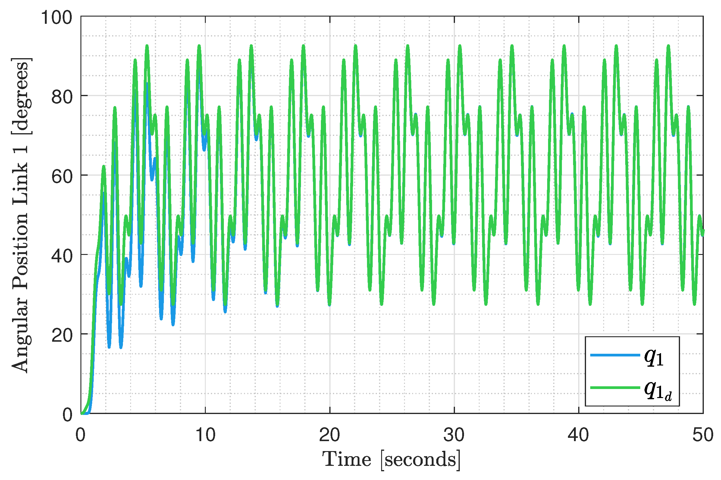
Lyapunov theory, as a formalism, generalizes the notion of energy in physical systems to any abstract dynamic set of differential equations via the so-called Lyapunov functions. Of course, this generalization preserves some properties, such as the total energy in a physical system being the sum of the individual energy in each of the subsystems that compose such a system. While passivity formalism established laws by which to obtain such a generalization of energy by conveniently performing combinations of the Lyapunov functions considered for each these subsystems. When a non-conservative force is considered, it can be treated as a bounded (not necessarily continuous) disturbance in feedback control. The fundamental result of such an approach is the fact that a Lyapunov function for a general system can be determined by solely adding the Lyapunov functions describing each of its subsystems. This approach is often referred to as an additive disturbance, and in this work, friction effects will be dealt with via two independent subsystems that identify time-varying coefficients, as described by (7). Now, considering the system in (1) with non-conservative forces due to friction model (2), as well as the results in the previous subsection, the proposed control law is given by
τ = Y q , q ˙ r , q ¨ r θ t + Y C q ˙ r θ ^ C t + Y v q ˙ r θ ^ v t K D s .
with update laws (37) for the first term and
θ ^ ˙ C t = Γ 2 Y C T q ˙ r s , Γ 2 = Γ 2 T > 0 ,
θ ^ ˙ v t = Γ 3 Y v T q ˙ r s , Γ 3 = Γ 3 T > 0 ,
for the second and third terms, respectively. Then, the election of the Lyapunov function is as follows:
V s , t = 1 2 s T M s + θ ˜ T Γ 1 θ ˜ + θ ˜ C T Γ 2 1 θ ˜ C + θ ˜ v T Γ 3 1 θ ˜ v .
The time derivative of (43) along the trajectories of the system results in
V ˙ s , t = s T τ Y q , q ˙ r , q ¨ r θ * f q ˙ , t + θ ˙ T Γ 1 1 θ ˜ + θ ˙ C T Γ 2 1 θ ˜ C + θ ˙ v T Γ 3 1 θ ˜ v .
Since f q ˙ , t ; q ˙ d = Y C q ˙ r θ C t + Y v q ˙ r θ v t , using (37), (41), and (42) leads to
V ˙ s , t = s T K D + F C t + F v t s e i 1 T κ e i 1 < 0 , s 0 , e i 0 .
Of course, the friction effects in (2) are physically bounded above and below by some finite constant because Coulomb-like friction effects are, at most equal, to the force causing movement. Mathematically, this translates into a saturation with a non-symmetric threshold given by
F C t = F C 1 , q ˙ t > 0 , 0 , q ˙ t = 0 , F C 2 , q ˙ t < 0 .
On the other hand, viscous-like friction effects are, at most, equal to a factor of the normal force that ensures static equilibrium, and are at least equal to the force sufficient to hold the movement of an object. Every value in between depends on the direction of movement, if it was already in movement or at rest, and the rate of velocity. Mathematically, the dependence of the state of a system on its history translates into a rate-dependent hysteresis. Thus, each time variant friction coefficient in (45) is bounded as follows:
k 1 = min F C 1 , F C 2 F C t max F C 1 , F C 2 = k 2
k 3 = inf t 0 t < F v t F v t sup t 0 t < F v t = k 4
Therefore, the time derivative in (39) satisfies
V ˙ s , t W 3 s = s T K D + k 2 + k 4 s < 0 .
Finally, since 0 < W 1 s V s , t W 2 s and V ˙ s , t W 3 s < 0 , the virtual velocity s tends to 0 as t . Now, from definition (28), q ˜ is exponentially bounded and will tend to 0 as t as well as q ˜ ˙ . This is sufficient to demonstrate that system
d d t q q ˙ = q ˙ M 1 q τ C q , q ˙ q ˙ g q f q ˙ , t ,
is uniformly asymptotically stable.

6. Results

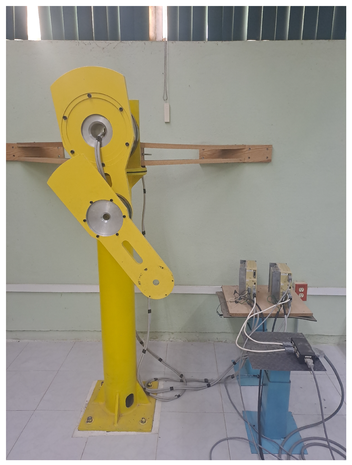
Experimental Test Implementation

The two-degree-of-freedom robot manipulator shown in Figure 3 was used as the physical plant for the experimental tests carried out using the following setup. All the links are actuated by direct-drive motors from Yokogawa Electric Corporation, model DM1A-200G for link 1 and model DM1B-030G for link 2. The motors are configured in torque mode, with a maximum torque of ± 200 N · m for link 1 and ± 30 N · m for link 2. The motors are equipped with relative encoders with a resolution of 1,024,000 and 655,360 pulses per revolution, respectively.
The digital implementation of the proposed controller and update law runs in MATLAB/Simulink using the Simulink Desktop Real-Time tool with a sampling period of 1 ms on a PC equipped with a Core i5 14,600K CPU, 32 gb of RAM, a RTX 3060 GPU, a 512 gb SSD M.2 for storage, and Windows 10 OS. The connection between the PC and the robot was carried out by a data acquisition card (DAQ) from Sensoray model 626 mounted on a PCI port on the motherboard of the PC and the drivers of each link from PARKER COMPUMOTOR, model DMG3-1200A for link 1 and DMG3-1030B for link 2. The DAQ sends a voltage signal representing each torque computed by the control law into analog inputs in the drivers. On the other hand, the drivers send a pulse train that replicates the signal from the encoders inside the motors to digital inputs in the DAQ. It is worth noting that the only custom-built devices in this setup are the links and the base stand of the robot; these were made by Centro de Investigación Científica y de Educación Superior de Ensenada for academic purposes.
The desired trajectories used in the experimental implementation tests are defined as follows:
q d 1 q d 2 = b 1 1 e d 1 t 3 + c 1 1 e d 1 t 3 sin ω 1 t + cos 3 ω 1 t + sin 5 ω 1 t b 2 1 e d 2 t 3 + c 2 1 e d 2 t 3 sin ω 2 t + cos 3 ω 2 t + sin 5 ω 2 t
where
b 1 = π 3 [ rad ] , b 2 = π 3 [ rad ] , c 1 = π 12 [ rad ] , c 2 = π 16 [ rad ]
d 1 = 0.3 1 s 3 , d 2 = 0.4 1 s 3 , ω 1 = 1.5 rad s , ω 2 = 1 rad s .
The choice on desired trajectories has two purposes: the first one is to provide a rather complicated tracking task and still show good performance compared to other controllers; the second one is to satisfy the persistent excitation for the first estimator in (19) by following the insight that three harmonics—i.e., at least three periodic functions with a common factor but different frequencies—are enough to excite all of the natural modes of a 2-DOF mechanical system; indeed, this is the physical meaning of persistent excitation. Of course, this excitation needs to be held for a finite period, but sine functions are periodic and harmonic; thus, experimentally, this condition is satisfied trivially after certain cycles. All the constant parameters in controller design are shown below:
Λ = 3 0 0 3 , λ f = 130 , Γ 1 = 0.23 0 0 0 0 0.86080155 0 0 0 0 0.65305335 0 0 0 0 0.3 .
κ = 1 0 0 1 , Γ 2 = 48 0 0 18.48 , Γ 3 = 36 0 0 6.15
Physical initial conditions were q 0 = 0 and q ˙ 0 = 0 , and the only prior information of the system is that l 1 = 0.313 [ m ] . The angular positions of each joint are shown in Figure 4 and Figure 5, respectively.
The angular position errors of each joint are shown in Figure 6 and Figure 7, respectively.
The torques applied at each joint are shown in Figure 8 and Figure 9, respectively.
Finally, the nominal vector of physical inertia and geometric parameters, i.e.,
θ * = θ 1 θ 2 θ 3 θ 4 = I 1 + m 1 l c 1 2 + I 2 + m 2 l c 2 2 + m 2 l 1 2 m 2 l c 2 I 2 + m 2 l c 2 2 m 1 l c 1 + m 2 l 1 ,
was estimated. The parameter estimates are shown in Figure 10, Figure 11, Figure 12 and Figure 13, respectively.
As seen in previous figures, all the elements in (52) tend to stay around their nominal constant values, respectively, since the desired trajectories in (51) were selected to satisfy (19), and their derivatives were bounded above by some finite number. Of course, the physical real parameters where known but were supposed to be unknown while designing the controller. On the other hand, friction coefficients were not exactly known a priori; instead, according to way the robot dynamics evolve when tracking the specific desired trajectories, both parts of (7) were determined by two independent estimators with their own update laws. The parameter estimates of Coulomb-like friction and viscous-like friction are shown in Figure 14 and Figure 15, respectively.
In both of the estimates, the coefficients associated with link 1 present a larger variation while tracking, this reflects the fact that the link has a significant threshold between the static regime compared to the dynamic regime due to a larger apparent area of contact that increases the adhesion between surfaces, while the second link only presents significant variation when a change in direction occurs at the maximum velocity of the link. A video of the experimental test was uploaded to YouTube: https://youtu.be/9AA2FeD3SRs (accessed on 20 March 2025).

7. Conclusions

In this manuscript, two important (but often underestimated) non-ideal non-linearities of friction phenomena are addressed to overcome the lack of a precise dynamic model of non-conservative forces in robot manipulators while preserving the passive mapping between the adaptation law and the parameter estimation error via additive disturbances theory. We put forward a technical proposal for two independent passive systems to take into account the anisotropy of typical Coulomb friction and the rate-dependent hysteresis generated in transition from one regime of viscous friction. Mathematical support for the decomposition of the conservative and non-conservative part into a novel linear parametrization is presented. This allows us to identify simple bounds for each regressor matrix and to satisfy the persistent excitation condition quite easily. Furthermore, simple quadratic Lyapunov functions for each estimator can be used in the stability analysis. The term of the adaptive computed torque used as control law, which can be seen in the in-disguise PD controller, uses the robust nature of the sliding mode approach to reject small changes in the additive disturbances, leading to a quite-good tracking performance in experimental tests. It is crucial to point out that in control theory applications, with the digital implementation of the controller, the discrete time domain is inherently induced and therefore a state transition between (quasi-)static and dynamic regimes. Finally, the proposed controller keeps the Lyapunov stability analysis simple as both friction phenomena are taken into account independently of each other and treated as additive disturbances that translate into an enhanced damping effect.

Author Contributions

Conceptualization, D.G.-H., J.S.-M. and V.S.; Software, D.G.-H. and I.G.; Validation, D.G.-H., J.S.-M. and V.S.; Formal analysis, D.G.-H.; Writing—original draft, D.G.-H.; Supervision, J.S.-M., V.S. and I.G. All authors have read and agreed to the published version of the manuscript.

Funding

This research was partially supported by Tecnologico Nacional de Mexico TecNM Projects 22483.25-P and LAGU-PYR-2025-23646, the net RICCA of TecNM, and PH.D. Student SECIHTI grant, CONACYT grant number 134534, postdoctoral fellow SECIHTI grant I1200/311/2023.

Data Availability Statement

Data are contained within the article.

Acknowledgments

This work was developed in the framework of the international network “Red internacional de control y cómputo aplicados” supported by Tecnológico Nacional de México (TecNM). This research was supported by “Secretaría de Ciencia, Humanidades, Tecnología e Innovación” and partially supported by TecNM Projects.

Conflicts of Interest

The authors declare no conflicts of interest.

References

  1. Slotine, J.J.E.; Li, W. Composite adaptive control of robot manipulators. Automatica 1989, 25, 509–519. [Google Scholar] [CrossRef]
  2. Nielsen, H.A.; Madsen, H. Modelling the heat consumption in district heating systems using a grey-box approach. Energy Build. 2006, 38, 63–71. [Google Scholar] [CrossRef]
  3. Slotine, J.J.E.; Li, W. On the Adaptive Control of Robot Manipulators. Int. J. Robot. Res. 1987, 6, 49–59. [Google Scholar] [CrossRef]
  4. Hastie, T.; Tibshirani, R. Varying-Coefficient Models. J. R. Stat. Soc. Ser. B (Methodol.) 1993, 55, 757–779. [Google Scholar] [CrossRef]
  5. Stokes, G. On the Variation of Gravity at the Surface of the Earth. In Mathematical and Physical Papers; Cambridge University Press: Cambridge, UK, 2009; pp. 131–171. [Google Scholar]
  6. Marques, F.; Flores, P.; Pimenta Claro, J.C.; Lankarani, H.M. A survey and comparison of several friction force models for dynamic analysis of multibody mechanical systems. Nonlinear Dyn. 2016, 86, 1407–1443. [Google Scholar] [CrossRef]
  7. Popova, E.; Popov, V.L. The research works of Coulomb and Amontons and generalized laws of friction. Friction 2015, 3, 183–190. [Google Scholar] [CrossRef]
  8. Armstrong-Hélouvry, B. Control of Machines with Friction, 1st ed.; Kluwer Academic Publishers: London, UK, 1991; pp. 24–35. [Google Scholar]
  9. Dahl, P.R. Solid Friction Damping of Mechanical Vibrations. AIAA J. 1976, 14, 1675–1682. [Google Scholar] [CrossRef]
  10. Olsson, H.; Åström, K.J.; Canudas de Wit, C.; Gäfvert, M.; Lischinsky, P. Friction Models and Friction Compensation. Eur. J. Control 1998, 4, 176–195. [Google Scholar] [CrossRef]
  11. Armstrong-Hélouvry, B.; Dupont, P.; Canudas de Wit, C. A Survey of Models, Analysis Tools and Compensation Methods for the Control of Machines with Friction. Automatica 1994, 30, 1083–1138. [Google Scholar] [CrossRef]
  12. Åström, K.J.; Canudas de Wit, C. Revisiting the LuGre Friction Model. IEEE Control Syst. Mag. 2008, 28, 101–114. [Google Scholar]
  13. Marques, F.; Woliński, Ł.; Wojtyra, M.; Flores, P.; Lankarani, H.M. An Investigation of a Novel LuGre-based Friction Force Model. Mech. Mach. Theory 2021, 166, 104493. [Google Scholar] [CrossRef]
  14. Niranjan, P.; Karinka, S.; Sairam, K.V.S.S.S.S.; Upadhya, A.; Shetty, S. Friction modeling in servo machines: A review. Int. J. Dynam. Control 2018, 6, 893–906. [Google Scholar] [CrossRef]
  15. Grami, S.; Okonkwo, P.C. Friction Compensation in Robot Manipulator Using Artificial Neural Network. In Advances in Automation, Signal Processing, Instrumentation, and Control; Komanapalli, V.L.N., Sivakumaran, N., Hampannavar, S., Eds.; Springer: Singapore, 2021; pp. 641–650. [Google Scholar]
  16. Sun, Y.; Liang, X.; Wan, Y. Tracking Control of Robot Manipulator with Friction Compensation Using Time-Delay Control and an Adaptive Fuzzy Logic System. Actuators 2023, 12, 184. [Google Scholar] [CrossRef]
  17. Ali, K.; Mehmood, A.; Iqbal, J. Fault-tolerant scheme for robotic manipulator—Nonlinear robust back-stepping control with friction compensation. PLoS ONE 2021, 16, e0256491. [Google Scholar] [CrossRef] [PubMed]
  18. Han, J.; Cheng, H.; Shan, X.; Liu, H.; Xiao, J.; Huang, T. A novel multi-pulse friction compensation strategy for hybrid robots. Mech. Mach. Theory 2024, 201, 105726. [Google Scholar] [CrossRef]
  19. Lewis, F.L.; Dawson, D.M.; Abdallah, C.T. Robot Manipulator Control: Theory and Practice, 2nd ed.; CRC Press: Boca Raton, FL, USA, 2003; pp. 125–136. [Google Scholar]
  20. Spong, M.W.; Hutchinson, S.; Vidyasagar, M. Robot Dynamics and Control, 2nd ed.; John Wiley & Sons, Inc.: Hoboken, NJ, USA, 2006; pp. 216–219. [Google Scholar]
  21. Rill, G.; Schaeffer, T.; Schuderer, M. LuGre or not LuGre. Multibody Syst. Dyn. 2024, 60, 191–218. [Google Scholar] [CrossRef]
  22. Kelly, R.; Santibáñez, V.; Loría, A. Control of Robot Manipulators in Joint Space, 1st ed.; Springer: London, UK, 2005; pp. 19–57, 95–101. [Google Scholar]
  23. Barahanov, N.; Ortega, R. Necessary and Sufficient Conditions for Passivity of the LuGre Friction Model. IEEE Trans. Autom. Control 2000, 45, 830–832. [Google Scholar] [CrossRef]
  24. Canudas-de-Wit, C.; Kelly, R. Passivity Analysis of a Motion Control for Robot Manipulators with Dynamic Friction. Asian J. Control 2007, 9, 30–36. [Google Scholar] [CrossRef]
  25. Istepanian, R.S.H.; Whidborne, J.F. Finite-Precision Computing for Digital Control Systems: Current Status and Future Paradigms. In Digital Controller Implementation and Fragility: A Modern Perspective; Istepanian, R.S.H., Whidborne, J.F., Eds.; Springer: London, UK, 2001; pp. 1–12. [Google Scholar]
  26. Soto, I.; Campa, R. Two-Loop Control of Redundant Manipulators: Analysis and Experiments on a 3-DOF Planar Arm. Int. J. Adv. Robot. Syst. 2013, 10, 85. [Google Scholar] [CrossRef]
  27. Sastry, S.S.; Boyd, M. Adaptive Control: Stability, Convergence and Robustness, 1st ed.; Prentice-Hall, Inc.: Englewood Cliffs, NJ, USA, 1989; p. 141. [Google Scholar]
  28. Boyd, S.; Sastry, S.S. Necessary and Sufficient Conditions for Parameter Convergence in Adaptive Control. Automatica 1986, 22, 629–639. [Google Scholar] [CrossRef]
  29. Gilbert, E.G.; Ha, I.J. An approach to nonlinear feedback control with applications to robotics. In Proceedings of the 22nd IEEE Conference on Decision and Control, San Antonio, TX, USA, 14–16 December 1983; pp. 879–884. [Google Scholar]
  30. Slotine, J.J.; Sastry, S.S. Tracking Control of Non-linear Systems Using Sliding Surfaces with Application to Robot Manipulators. In Proceedings of the 1983 American Control Conference, San Francisco, CA, USA, 22–24 June 1983; pp. 132–135. [Google Scholar]
Figure 1. Conceptual representation of friction phenomenon.
Actuators 14 00237 g001
Figure 2. Diagram of the 2-DOF robot manipulator [26].
Actuators 14 00237 g002
Figure 3. Two-degree-of-freedom robotic arm and motor drivers used for the experimental tests.
Actuators 14 00237 g003
Figure 4. Angular position for joint 1.
Actuators 14 00237 g004
Figure 5. Angular position for joint 2.
Actuators 14 00237 g005
Figure 6. Angular position error for joint 1.
Actuators 14 00237 g006
Figure 7. Angular position error for joint 2.
Actuators 14 00237 g007
Figure 8. Torque applied at joint 1.
Actuators 14 00237 g008
Figure 9. Torque applied at joint 2.
Actuators 14 00237 g009
Figure 10. Evolution of the estimated parameter θ 1 .
Actuators 14 00237 g010
Figure 11. Evolution of the estimated parameter θ 2 .
Actuators 14 00237 g011
Figure 12. Evolution of the estimated parameter θ 3 .
Actuators 14 00237 g012
Figure 13. Evolution of the estimated parameter θ 4 .
Actuators 14 00237 g013
Figure 14. Evolution of the estimated Coulomb-like friction coefficient f C 1 and f C 2 .
Actuators 14 00237 g014
Figure 15. Evolution of the estimated viscous-like friction coefficient f v 1 and f v 2 .
Actuators 14 00237 g015
Table 1. Physical parameters of the 2-DOF robot manipulator.
DescriptionNotationUnits
Length of link 1 l 1 m
Length of link 2 l 2 m
Distance to the center of mass of link 1 l c 1 m
Distance to the center of mass of link 2 l c 2 m
Mass of link 1 m 1 kg
Mass of link 2 m 2 kg
Inertia related to center of mass of link 1 I 1 kg · m 2
Inertia related to center of mass of link 2 I 2 kg · m 2
Acceleration due to gravityg m s 2
Disclaimer/Publisher’s Note: The statements, opinions and data contained in all publications are solely those of the individual author(s) and contributor(s) and not of MDPI and/or the editor(s). MDPI and/or the editor(s) disclaim responsibility for any injury to people or property resulting from any ideas, methods, instructions or products referred to in the content.

