Fixed-Time Adaptive Event-Triggered Control for Uncertain Nonlinear Systems Under Full-State Constraints

Abstract

The problem of adaptive event-triggered control for uncertain nonlinear systems with full-state constraints was investigated. State constraints can significantly affect system performance, especially when time-varying external disturbances are present, potentially leading to instability. Thus, a fixed-time disturbance observer was designed. It estimated unknown uncertainties within a predetermined time. Meanwhile, an asymmetric barrier Lyapunov function was developed. It ensured the stability of the system state under constraints. Furthermore, to reduce the utilization rate of the system’s communication resources, an adaptive event-triggered control scheme was proposed, and an integrated control method was established to preset the convergence time of the system’s state error, greatly improving the convergence speed. Theoretical analysis and simulations demonstrated the effectiveness of the proposed approach. The results show that the system achieved stable control within a fixed time, even under full-state constraints and external disturbances, while using fewer communication resources.

1. Introduction

In practical engineering, most mechanical systems can be modeled as nonlinear systems, including drones, standard systems, robotic arms, and underwater vehicles. Over the past two decades, the control of nonlinear systems [1,2,3,4,5,6] has been a significant area of research in modern control theory. These systems typically exhibit complex dynamic behaviors and are influenced by various uncertainties and external disturbances, making control tasks highly challenging. There are still numerous scientifically significant and practically valuable problems in this research field that need to be addressed. Many scholars have conducted various studies on the control of nonlinear systems [7,8,9]. Despite the progress made in these studies, conventional control methods still have limitations in dealing with system uncertainties and external disturbances. Wang et al. [10] considered continuous bounded switching for the finite-time attitude stabilisation control of spacecraft systems with actuator saturation problems. However, the limitations of finite-time stabilization control, which is affected by the initial state conditions, result in its inadequacy for certain practical engineering applications. To eliminate the effect of the initial state, in [11], Polyakov proposed a fixed-time stabilisation control method. The method ensures that the convergence time of the system under different initial conditions remains within a definite neighbourhood. Scholars have used this advantage of the method to propose classical fixed-time control methods for various system structures [12,13,14,15,16].

Although these studies have made some progress, the aforementioned methods still have limitations in dealing with uncertain gains. When machinery operates in a real environment, it inevitably encounters gain uncertainties, which are often nonlinear, time-varying, and unknowable functions. Several researchers have used different methods [17,18,19,20,21,22,23,24,25,26,27] to compensate for these unknown uncertainties to reduce or eliminate their effects on the system. Wang et al. [28] developed a fixed-time convergence method utilizing adaptive fuzzy control techniques. Zhuang et al. [29] designed an Adaptive Sliding-Mode Disturbance Observer (ASMDO) for uncertain robotic systems. Moreover, considering the actuator saturation problem in robotic systems, they developed a new adaptive fixed-time auxiliary system. This enabled faster fixed-time high-precision tracking control for uncertain robotic systems.

All of the above methods have achieved significant results in dealing with unknown perturbation disturbances, but they may no longer be applicable when the inputs and outputs of a system are generally constrained. State constraints are dictated by physical and safety requirements in many practical applications. The proper consideration and handling of these constraints can effectively improve the performance and safety of a system, thus ensuring that all design requirements are met during operation.

In addition, under the constraints on communication resources, traditional control strategies usually require the continuous updating of control signals, which not only increases the computational complexity but also leads to excessive communication bandwidth consumption. To overcome these limitations, event-triggered control strategies [30,31,32,33,34,35,36] have been proposed in recent years. These strategies aim to update the control signals only when necessary, thus reducing unnecessary computational and communication burdens. Zhou et al. [37] proposed self-triggered and event-triggered control methods and designed novel event-triggered sampling and self-triggered sampling based on dynamic quantisation parameters. Nonetheless, this method faces challenges when applied to uncertain nonlinear systems. Zhang et al. [38] addressed the issues of input saturation and unsaturation in discrete-time systems. They designed a low-frequency event-triggered mechanism based on cumulative errors and extended the looped functional method to achieve the collaborative design of control gains and event-triggered parameters. The effectiveness of this approach was verified using an unstable reactor system and an inverted pendulum system.

Inspired by previous studies, this paper investigated an adaptive event-triggered control strategy for uncertain nonlinear systems with complete state constraints. In this paper, we designed a fixed-time disturbance observer to estimate and compensate for unknown external disturbances in the system, ensuring that the control strategy remains effective despite these disturbances. Our approach employs a logarithmic barrier Lyapunov function to handle the state constraints, ensuring that the system state remains within a predetermined range throughout the control process. We then propose an adaptive event-triggering mechanism to save the system’s communication resources. The main contributions of this paper are as follows:

• To enhance the system’s robustness and stability, we innovatively designed a fixed-time disturbance observer to estimate and compensate for the uncertainty gain while employing a logarithmic barrier Lyapunov function to manage state constraints, thereby ensuring stability under these constraints.
• An adaptive event-triggering mechanism is proposed which significantly reduces the computational and communication burden by reducing the update frequency of the control signal.

The rest of this article is organized as follows. Section 2 introduces the system model and preparatory knowledge; Section 3 describes in detail the designed controller and its stability analysis; Section 4 describes how we verified the validity of the proposed methodology through simulation experiments; and Section 5 summarises the research work in this paper and proposes future research directions.

2. Model Description and Preliminaries

Model Description

Consider the following nonlinear system:

$$\left\{\begin{array}{c}{\dot{x}}_i=f_i\left({\overline{x}}_i\right)+g_i\left({\overline{x}}_i\right)x_{i+1}\hfill \\ ⋮\hfill \\ {\dot{x}}_n=f_n\left({\overline{x}}_n\right)+g_n\left({\overline{x}}_n\right)u\left(t\right)+d\hfill \\ y=x_1\hfill \end{array}\right.$$

(1)

where $i=1,2,\dots ,n-1$; ${\overline{x}}_i={[x_1,x_2,\dots ,x_j]}^T\in {\mathbb{R}}^j$$(j=1,2,\dots ,n)$ represents the state vector; d represents the total disturbance; $f_i\left({\overline{x}}_i\right)$ and $g_i\left({\overline{x}}_i\right)$ are unknown smooth functions; and u denotes the control input. The output $x_1$ and the desired value $x_d$ satisfy the asymmetric constraints $-k_{ax}<x_1<k_{bx}$ and $-k_{ad}<x_d<k_{bd}$, where $k_{ax}$ and $k_{ad}$ and $k_{bx}$ and $k_{bd}$ are known constants. Defining the error in $x_1$ as $e_1=x_d-x_1$, we have $-k_{a1}<e_1<k_{b1}$, where $k_{a1}=k_{ax}+x_{1d}$ and $k_{b1}=k_{bx}-x_{1d}$.

The objective of this paper was to address the combined effects of output constraints and external disturbances. By utilizing a fixed-time disturbance observer, logarithmic barrier Lyapunov function, and an adaptive event-triggered mechanism, we designed a fixed-time backstepping controller. This controller ensures the bounded stability of a system within a fixed time, allowing the output $x_1$ to track its reference command $x_d$ within a fixed time while satisfying the constraint conditions.

Before describing how we designed the controller, we provide the following Lemmas and Assumptions.

Lemma 1

(see [11]). Assume that there exists a continuously differentiable function, $V:{\mathbb{R}}^n\to {\mathbb{R}}_{+}\cup \left\{0\right\}$, that satisfies

$$V\left(x\right)=0\iff x=0$$

(2)

For any $x\left(t\right)$, the following inequality holds:

$$\dot{V}\left(x\right)\le -{\gamma }_1{V}^{\alpha }\left(x\right)-{\gamma }_2{V}^{\beta }\left(x\right)$$

(3)

Therefore, the system is globally stable at a fixed time. Where ${\gamma }_1,{\gamma }_2,\alpha ,\beta ,$ and ϑ are positive constants, $0<\alpha <1$, $\beta >1$, and $0<\vartheta <1$. Thus, the system achieves fixed-time stability, with the convergence time T bounded by

$$T\le T_{max}:={\displaystyle \frac{1}{{\gamma }_1(1-\alpha )}}+{\displaystyle \frac{1}{{\gamma }_2(\beta -1)}}$$

(4)

For any $x\left(t\right)$, the following inequality holds:

$$\dot{V}\left(x\right)\le -{\gamma }_1{V}^{\alpha }\left(x\right)-{\gamma }_2{V}^{\beta }\left(x\right)+\vartheta$$

(5)

Therefore, the system is actually stable at a fixed time, and the convergence time T is bounded by

$$T\le T_{max}:={\displaystyle \frac{1}{{\gamma }_1\theta (1-\alpha )}}+{\displaystyle \frac{1}{{\gamma }_2\theta (\beta -1)}}$$

(6)

The domain of convergence of the system is

$$\mathrm{\Xi }=\left\{V\left(x\right)\le min\left\{{\left[{\displaystyle \frac{\vartheta }{{\gamma }_1(1-\theta )}}\right]}^{{\displaystyle \frac{1}{\alpha }}},{\left[{\displaystyle \frac{\vartheta }{{\gamma }_2(1-\theta )}}\right]}^{{\displaystyle \frac{1}{\beta }}}\right\}\right\}$$

(7)

where θ is a positive constant satisfying $0<\theta <1$.

Lemma 2

(see [39]). For any $x,y\in \mathbb{R}$, if $q>0,a>1$, and $b>1$ such that ${\displaystyle \frac{1}{a}}+{\displaystyle \frac{1}{b}}=1$, the following inequality holds:

$$xy\le {\displaystyle \frac{q^a}{a}}{|x|}^a+{\displaystyle \frac{1}{b{q}^b}}{|y|}^b$$

(8)

Lemma 3

(see [40]). Let ${\xi }_1,\dots ,{\xi }_n\ge 0$. If $0<{\sigma }_1<1$ and ${\sigma }_2>1$, the following inequalities are satisfied:

$${\left(\sum _{\ell =1}^n{\xi }_{\ell }^{{\sigma }_1}\right)}^{{\displaystyle \frac{1}{{\sigma }_1}}}\ge \sum _{\ell =1}^n{\xi }_{\ell }$$

(9)

$${\left(\sum _{\ell =1}^n{\xi }_{\ell }^{{\sigma }_2}\right)}^{{\displaystyle \frac{1}{{\sigma }_2}}}\ge n^{1-{\displaystyle \frac{1}{{\sigma }_2}}}\sum _{\ell =1}^n{\xi }_{\ell }$$

(10)

Lemma 4

(see [41]). For any $|\eta |<1$ and any positive integer, m, the following inequality is satisfied:

$$log\left({\displaystyle \frac{1}{1-{\eta }^{2m}}}\right)\le {\displaystyle \frac{{\eta }^{2m}}{1-{\eta }^{2m}}}$$

(11)

Lemma 5

(see [42]). For any $\upsilon \in \mathbb{R}$ and $\tau >0$, the following inequalities hold:

$$\left\{\begin{array}{c}-\upsilon tanh\left({\displaystyle \frac{\upsilon }{\tau }}\right)\le 0,\hfill \\ 0\le |\upsilon |-\upsilon tanh\left({\displaystyle \frac{\upsilon }{\tau }}\right)\le 0.2785\tau \hfill \end{array}\right.$$

(12)

Assumption A1.

There exist positive constants, $g_{im}$ and $g_{iM}$, such that the following inequality holds:

$$0<g_{im}\le g_i\left({\overline{x}}_i\right)\le g_{iM}<\infty$$

(13)

Assumption A2.

The external disturbance $d\left(t\right)$ satisfies

$$|d\left(t\right)|\le D_0$$

(14)

$$|\dot{d}\left(t\right)|\le D_1$$

(15)

where $D_0$ and $D_1$ are unknown positive constants.

Assumption A3.

For the disturbance observer, there exists a valid range for the disturbance estimate $\widehat{d}$, such that $|\widehat{d}|<D_2$, where $D_2$ is unknown positive constant.

Assumption A4.

For the reference command $x_d\left(t\right)$, there exist known constraints, $k_{ad}$ and $k_{bd}$, such that

$$-k_{ad}<x_d\left(t\right)<k_{bd}$$

(16)

3. Developing Controllers and Analyzing Stability

3.1. The Construction of the FTDO

This section proposes a design method for a fixed-time disturbance observer to eliminate the influence of external mismatched disturbance signals with unknown upper bounds on the system.

The error of the bootstrap estimate is defined as

$$\tilde{d}=d-\widehat{d}$$

(17)

where d represents the actual unknown aggregate disturbance and $\widehat{d}$ is the estimated disturbance observed by the observer.

The design of the disturbance observer is as follows:

$$\dot{\widehat{d}}=k_d(c_1{sign}^{\iota }\left(\tilde{d}\right)+c_2{\tilde{d}}^{\varsigma })$$

(18)

where $k_d$, $c_1$, and $c_2$ are positive parameters to be designed, and $0<\iota <1$ and $\varsigma >1$. The formula $sign$ is expressed as $sig{n}^{\iota }\left(a\right)=sig\left(a\right){|a|}^{\iota }$.

3.2. The Stability Analysis of the FTDO

Theorem 1.

If the fixed-time perturbation observer (18) is used in the system, the estimation error of the observer regarding the set total perturbation in the system is guaranteed to converge within a fixed time, $T_1$.

Proof. 

Define the first Lyapunov function candidate as follows:

$$V_d={\displaystyle \frac{1}{2}}{\tilde{d}}^2$$

(19)

and the time derivative is expressed as

$${\dot{V}}_d=\tilde{d}\dot{\tilde{d}}$$

(20)

By combining this with Equations (17) and (18), the following expression is obtained:

$$\begin{array}{cc}\hfill {\dot{V}}_d& =\tilde{d}\dot{\tilde{d}}\hfill \\ \hfill & =\tilde{d}(\dot{d}-\dot{\widehat{d}})\hfill \\ \hfill & =\tilde{d}(\dot{d}-k_d(c_1{sign}^{\iota }\left(\tilde{d}\right)+c_2{\tilde{d}}^{\varsigma }))\hfill \\ \hfill & =\tilde{d}\dot{d}-k_d{c}_1{sign}^{\iota }\left(\tilde{d}\right)\tilde{d}-k_d{c}_2{\tilde{d}}^{1+\varsigma }\hfill \end{array}$$

(21)

Using the inequality $\tilde{d}\dot{d}\le |\tilde{d}||\dot{d}|$ and Assumption 2, we obtain the following results:

$$\tilde{d}\dot{d}\le |\tilde{d}|D_1$$

(22)

Substituting Equation (21) into Equation (22), we obtain

$$\begin{array}{cc}\hfill {\dot{V}}_d& \le |\tilde{d}|D_1-k_d{c}_1{sign}^{\iota }\left(\tilde{d}\right)\tilde{d}-k_d{c}_2{sign}^{\varsigma }\left(\tilde{d}\right)\tilde{d}\hfill \\ \hfill & \le |\tilde{d}|D_1-k_d{c}_{1}sig\left(\tilde{d}\right)|\tilde{d}{|}^{\iota }\tilde{d}-k_d{c}_{2}sig\left(\tilde{d}\right){|\tilde{d}|}^{\varsigma }\tilde{d}\hfill \\ \hfill & \le |\tilde{d}|D_1-k_d{c}_1|\tilde{d}{|}^{\iota +1}-k_d{c}_2{|\tilde{d}|}^{1+\varsigma }\hfill \\ \hfill & \le |\tilde{d}|D_1-k_d{c}_1{\left({\tilde{d}}^2\right)}^{{\displaystyle \frac{\iota +1}{2}}}-k_d{c}_2{\left({\tilde{d}}^2\right)}^{{\displaystyle \frac{1+\varsigma }{2}}}\hfill \\ \hfill & \le -k_d{c}_1{\left({\displaystyle \frac{1}{2}}{\tilde{d}}^2\right)}^{{\displaystyle \frac{\iota +1}{2}}}-k_d{c}_2{\left({\displaystyle \frac{1}{2}}{\tilde{d}}^2\right)}^{{\displaystyle \frac{1+\varsigma }{2}}}+\vartheta \hfill \\ \hfill & \le -2^{{\displaystyle \frac{\iota +1}{2}}}{k}_d{c}_1{\left({\displaystyle \frac{1}{2}}{\tilde{d}}^2\right)}^{{\displaystyle \frac{\iota +1}{2}}}-2^{{\displaystyle \frac{1+\varsigma }{2}}}{k}_d{c}_2{\left({\displaystyle \frac{1}{2}}{\tilde{d}}^2\right)}^{{\displaystyle \frac{1+\varsigma }{2}}}+\vartheta \hfill \end{array}$$

(23)

According to Lemma 1, it can be concluded that $\tilde{d}$ exhibits fixed-time stability, with the convergence time $T_1$ satisfying the following condition:

$$T_1\le {\displaystyle \frac{2^{\frac{1-\iota }{2}}}{k_d{c}_1\theta (1-\iota )}}+{\displaystyle \frac{2^{\frac{1-\varsigma }{2}}}{k_d{c}_1\theta (\varsigma -1)}}$$

(24)

The domain of convergence of $\tilde{d}$ is given by

$$V\left(\tilde{d}\right)=\left\{V\left(x\right)\le min\left\{{\left[{\displaystyle \frac{\vartheta }{2^{\frac{\iota +1}{2}}{k}_d{c}_1(1-\theta )}}\right]}^{{\displaystyle \frac{2}{\iota +1}}},{\left[{\displaystyle \frac{\vartheta }{2^{\frac{\varsigma +1}{2}}{k}_d{c}_2(1-\theta )}}\right]}^{{\displaystyle \frac{2}{\zeta +1}}}\right\}\right\}$$

(25)

Therefore, when $t\ge T_1$, the observer’s estimation error $\tilde{d}$ converges within a predetermined fixed time.

Hence, Theorem 1 is proved. □

3.3. Design of Event-Driven Fixed-Time Controller

Utilizing the backstepping technique, a fixed-time controller for a nonlinear system was expertly designed to ensure precise reference path tracking and the fixed-time convergence of the tracking error. To minimize communication resource consumption and avoid the Zeno phenomenon, an event-triggered mechanism was incorporated into the controller.

The error system is initially defined as follows:

$$\left\{\begin{array}{c}{e}_1=x_1-x_d\hfill \\ e_2=x_2-{\alpha }_1\hfill \\ ⋮\hfill \\ e_n=x_n-{\alpha }_{n-1}\hfill \end{array}\right.$$

(26)

where $\alpha ={[{\alpha }_1,{\alpha }_2,\dots ,{\alpha }_{n-1}]}^{\mathrm{T}}$ represents the virtual control law to be constructed. From Equations (1) and (26), we can derive the following:

$$\begin{array}{cc}\hfill {\dot{e}}_1& ={\dot{x}}_1-{\dot{x}}_d\hfill \\ \hfill & =f_1+g_1{x}_2-{\dot{x}}_d\hfill \end{array}$$

(27)

Step 1: The following logarithmic barrier Lyapunov function is selected:

$$V_1={\displaystyle \frac{q\left(e_1\right)}{2r}}ln{\displaystyle \frac{k_b^{2r}}{k_b^{2r}-e_1^{2r}}}+{\displaystyle \frac{1-q\left(e_1\right)}{2r}}ln{\displaystyle \frac{k_a^{2r}}{k_a^{2r}-e_1^{2r}}}$$

(28)

where r is a positive integer and $2r\ge n$, and the function $q\left(e_1\right)$ is defined as

$$q\left(e_1\right)=\left\{\begin{array}{cc}1,\hfill & e_1>0\hfill \\ 0,\hfill & e_1\le 0\hfill \end{array}\right.$$

(29)

Differentiating $V_1$ yields the following result:

$$\begin{array}{cc}\hfill {\dot{V}}_1=& {\displaystyle \frac{q\left(e_1\right)e_1^{2r-1}}{k_b^{2r}-e_1^{2r}}}[f_1+g_1{x}_2-{\dot{x}}_{1d}]\hfill \\ \hfill & +{\displaystyle \frac{(1-q\left(e_1\right))e_1^{2r-1}}{k_a^{2r}-e_1^{2r}}}[f_1+g_1{x}_2-{\dot{x}}_{1d}]\hfill \end{array}$$

(30)

Let ${\mathrm{\Omega }}_i$ be defined as follows:

$${\mathrm{\Omega }}_i={\displaystyle \frac{q\left(e_i\right)}{k_b^{2r}-e_i^{2r}}}+{\displaystyle \frac{1-q\left(e_i\right)}{k_a^{2r}-e_i^{2r}}}$$

(31)

Then, the expression for ${\alpha }_1$ is given by

$$\begin{array}{cc}\hfill {\alpha }_1=& -g_1^{-1}(k_{11}{\mathrm{\Omega }}_1^{{\displaystyle \frac{v-1}{2}}}{e}_1^{r(v-1)+1}+k_{12}{\mathrm{\Omega }}_1^{{\displaystyle \frac{w-1}{2}}}{e}_1^{r(w-1)+1}\hfill \\ \hfill & +g_1{e}_1^{{\displaystyle \frac{2r-1}{2r}}}+f_1-{\dot{x}}_{1d})\hfill \end{array}$$

(32)

where $0<v<1$, $w>1$, and $k_{11}$ and $k_{12}$ are parameters to be designed. By substituting Equations (31) and (32) into $\dot{V_1}$, the following result is obtained:

$$\begin{array}{cc}\hfill {\dot{V}}_1=& {\mathrm{\Omega }}_1{g}_1{e}_1^{2r-1}{e}_2-{\displaystyle \frac{2r-1}{2r}}{\mathrm{\Omega }}_1{g}_1{e}_1^{2r}\hfill \\ \hfill & -k_{11}{\mathrm{\Omega }}_1^{{\displaystyle \frac{v+1}{2}}}{e}_1^{r(v+1)}-k_{12}{\mathrm{\Omega }}_1^{{\displaystyle \frac{w+1}{2}}}{e}_1^{r(w+1)}\hfill \end{array}$$

(33)

According to Lemma 2, it follows that

$$\begin{array}{cc}\hfill {\dot{V}}_1\le & -k_{11}{\mathrm{\Omega }}_1^{{\displaystyle \frac{v+1}{2}}}{e}_1^{r(v+1)}-k_{12}{\mathrm{\Omega }}_1^{{\displaystyle \frac{w+1}{2}}}{e}_1^{r(w+1)}\hfill \\ \hfill & +{\displaystyle \frac{1}{2r}}{\mathrm{\Omega }}_1{g}_1{e}_2^{2r}\hfill \end{array}$$

(34)

Step 2: According to Equation (26), the time derivative of $e_2$ is given by

$$\begin{array}{c}\hfill {\dot{e}}_2=f_2+g_2{x}_3-{\dot{\alpha }}_1\end{array}$$

(35)

Then, the following logarithmic barrier Lyapunov function is selected:

$$V_2=V_1+{\displaystyle \frac{q\left(e_2\right)}{2r}}ln{\displaystyle \frac{k_b^{2r}}{k_b^{2r}-e_2^{2r}}}+{\displaystyle \frac{1-q\left(e_2\right)}{2r}}ln{\displaystyle \frac{k_a^{2r}}{k_a^{2r}-e_2^{2r}}}$$

(36)

Its time derivative is given by

$$\begin{array}{cc}\hfill {\dot{V}}_2=& {\dot{V}}_1+{\displaystyle \frac{q\left(e_2\right)e_2^{2r-1}}{k_b^{2r}-e_2^{2r}}}[f_2+g_2{x}_3-{\dot{\alpha }}_1]\hfill \\ \hfill & +{\displaystyle \frac{\left(1-q\left(e_2\right)\right)e_2^{2r-1}}{k_a^{2r}-e_2^{2r}}}[f_2+g_2{x}_3-{\dot{\alpha }}_1]\hfill \end{array}$$

(37)

Based on Equation (26), $e_3=x_3-{\alpha }_2$, and the virtual control law ${\alpha }_2$ is designed as follows:

$$\begin{array}{cc}\hfill {\alpha }_2=& -g_2^{-1}(k_{21}{\mathrm{\Omega }}_2^{{\displaystyle \frac{v-1}{2}}}{e}_2^{r(v-1)+1}+k_{22}{\mathrm{\Omega }}_2^{{\displaystyle \frac{w-1}{2}}}{e}_2^{r(w-1)+1}\hfill \\ \hfill & +{\displaystyle \frac{2r-1}{2r}}{g}_2{e}_2+f_2-{\dot{\alpha }}_1+{\displaystyle \frac{1}{2r}}{\mathrm{\Omega }}_2^{-1}{\mathrm{\Omega }}_1{g}_1{e}_2)\hfill \end{array}$$

(38)

Then, using ${\alpha }_2$ and Lemma 2, ${\dot{V}}_2$ can be expressed as

$$\begin{array}{cc}\hfill {\dot{V}}_2\le & {\displaystyle \frac{1}{2r}}{\mathrm{\Omega }}_2{g}_2{e}_3^{2r}-k_{11}{\mathrm{\Omega }}_1^{{\displaystyle \frac{v+1}{2}}}{e}_1^{r(v+1)}-k_{12}{\mathrm{\Omega }}_1^{{\displaystyle \frac{w+1}{2}}}{e}_1^{r(w+1)}\hfill \\ \hfill & -k_{21}{\mathrm{\Omega }}_2^{{\displaystyle \frac{v+1}{2}}}{e}_2^{r(v+1)}-k_{22}{\mathrm{\Omega }}_2^{{\displaystyle \frac{w+1}{2}}}{e}_2^{r(w+1)}\hfill \end{array}$$

(39)

Step i $(3\le i\le n-1)$: According to Equation (26), the time derivative of $e_i$ is given by

$$\begin{array}{c}\hfill {\dot{e}}_i=f_i+g_i{x}_{i+1}-{\dot{\alpha }}_i\end{array}$$

(40)

and the virtual control law ${\alpha }_i$ is designed as follows:

$$\begin{array}{cc}\hfill {\alpha }_i=& -g_i^{-1}(k_{i1}{\mathrm{\Omega }}_i^{{\displaystyle \frac{v-1}{2}}}{e}_i^{r(v-1)+1}+k_{i2}{\mathrm{\Omega }}_i^{{\displaystyle \frac{w-1}{2}}}{e}_i^{r(w-1)+1}\hfill \\ \hfill & +{\displaystyle \frac{2r-1}{2r}}{g}_i{e}_i+f_i-{\dot{\alpha }}_{i-1}+{\displaystyle \frac{1}{2r}}{\mathrm{\Omega }}_i^{-1}{\mathrm{\Omega }}_{i-1}{g}_{i-1}{e}_i)\hfill \end{array}$$

(41)

The following logarithmic barrier Lyapunov function is selected:

$$\begin{array}{cc}\hfill V_i=& V_{i-1}+{\displaystyle \frac{q\left(e_i\right)}{2r}}ln{\displaystyle \frac{k_b^{2r}}{k_b^{2r}-e_i^{2r}}}\hfill \\ \hfill & +{\displaystyle \frac{1-q\left(e_i\right)}{2r}}ln{\displaystyle \frac{k_a^{2r}}{k_a^{2r}-e_i^{2r}}}\hfill \end{array}$$

(42)

Applying ${\alpha }_i$ and Lemma 2, the relationship for the $V_i$ derivative can be obtained as follows:

$$\begin{array}{cc}\hfill {\dot{V}}_i\le & {\displaystyle \frac{1}{2r}}{\mathrm{\Omega }}_i{g}_i{e}_{i+1}^{2r}-\sum _{j=1}^i{k}_{j1}{\mathrm{\Omega }}_j^{{\displaystyle \frac{v+1}{2}}}{e}_j^{r(v+1)}\hfill \\ \hfill & -\sum _{j=1}^i{k}_{j2}{\mathrm{\Omega }}_j^{{\displaystyle \frac{w+1}{2}}}{e}_j^{r(w+1)}\hfill \end{array}$$

(43)

Step n: In this step, the virtual control input $\overline{u}\left(t\right)$ and the actual control input $u\left(t\right)$ will be designed. The time derivative of $e_n$ is given by

$$\begin{array}{c}\hfill {\dot{e}}_n=f_n+g_{n}u+d-{\dot{\alpha }}_{n-1}\end{array}$$

(44)

The following logarithmic barrier Lyapunov function is selected:

$$\begin{array}{cc}\hfill V_n=& V_{n-1}+{\displaystyle \frac{q\left(e_n\right)}{2r}}ln{\displaystyle \frac{k_b^{2r}}{k_b^{2r}-e_n^{2r}}}\hfill \\ \hfill & +{\displaystyle \frac{1-q\left(e_n\right)}{2r}}ln{\displaystyle \frac{k_a^{2r}}{k_a^{2r}-e_n^{2r}}}\hfill \end{array}$$

(45)

Differentiating $V_n$ yields the following result:

$$\begin{array}{cc}\hfill {\dot{V}}_n=& {\dot{V}}_{n-1}+{\mathrm{\Omega }}_n{e}_n^{2r-1}\left[f_n+g_{n}u+d-{\dot{\alpha }}_{n-1}\right]\hfill \end{array}$$

(46)

The event-triggered mechanism is designed as follows:

$$\left\{\begin{array}{c}\varpi =-\overline{u}tanh\left({\displaystyle \frac{e_n\overline{u}}{\kappa }}\right)(1+\rho )-{\displaystyle \frac{(1+\rho )e_n}{2{(1-\rho )}^2}}\hfill \\ u=\varpi \left(t_{i,k}\right),\forall t\in [t_{i,k},t_{i,k+1})\hfill \\ t_{i,k+1}=inf\left\{t\in R|\left|e_m\left(t\right)\right|\ge \rho u+h\right\}\hfill \end{array}\right.$$

(47)

where, inf {·} denotes the infimum, $e_m\left(t\right)=\varpi \left(t\right)-u\left(t\right)$ represents the measurement error, $\overline{u}$ is the designed virtual control law, and the design parameters of the control law satisfy $\kappa >0$, and $\rho$ and h satisfy the following equations:

$$\rho =\left\{\begin{array}{cc}{\lambda }_1-ϵsign\left(\mathrm{\Delta }\left(e_n\right)\right),\hfill & |e_n|>\mathrm{\Phi }\hfill \\ {\lambda }_2-ϵsign\left(\mathrm{\Delta }\left(e_n\right)\right),\hfill & |e_n|\le \mathrm{\Phi }\hfill \end{array}\right.$$

(48)

$$h=\left\{\begin{array}{cc}{\lambda }_3-ϵsign\left(\mathrm{\Delta }\left(e_n\right)\right),\hfill & |e_n|>\mathrm{\Phi }\hfill \\ {\lambda }_4-ϵsign\left(\mathrm{\Delta }\left(e_n\right)\right),\hfill & |e_n|\le \mathrm{\Phi }\hfill \end{array}\right.$$

(49)

where $0<{\lambda }_1,{\lambda }_2,ϵ<1$ and ${\lambda }_3,{\lambda }_4>0$, $\mathrm{\Delta }\left(e_n\right)$ is expressed as the rate of change of $e_n$, and $\mathrm{\Phi }$ is expressed as a threshold value of the error to be set. The event trigger times are denoted as $t_{i,k+1}$, with $K\in {\mathbb{Z}}^{+}$. The event-triggered mechanism is defined as follows: From the trigger time $t_{i,k}$ to the next trigger time $t_{i,k+1}$, the control input $\overline{u}$ remains at its value at $t_{i,k}$ until the next trigger time when the system updates the control input. The control input is updated only if the condition $|e_m\left(t\right)|\ge \rho u+h$ is satisfied. Selecting appropriate parameters can reduce the frequency of control input updates, thereby reducing resource consumption. Based on Equation (47), it follows that

$$\varpi =(1+{\xi }_2\left(t\right)\rho )u\left(t\right)+{\xi }_1\left(t\right)h$$

(50)

where $t\in [t_{i,k},t_{i,k+1})$ and $|{\xi }_1|,|{\xi }_2|\le 1$ are time-varying parameters. Furthermore, the following equation can be derived:

$$u={\displaystyle \frac{\varpi \left(t\right)-{\xi }_1\left(t\right)h}{1+{\xi }_2\left(t\right)\rho }}$$

(51)

Thus, the following relationship holds:

$$\begin{array}{cc}\hfill e_n^{2r-1}u=& -e_n^{2r-1}\left\{{\displaystyle \frac{1+\rho }{1+{\xi }_2\rho }}\left[\overline{u}tanh({\displaystyle \frac{e_n^{2r-1}\overline{u}}{\kappa }})\right]\right\}\hfill \\ \hfill & -{\displaystyle \frac{(1+\rho )e_n^{2r}}{2[1+{\xi }_2\left(t\right)\rho ]{(1-\rho )}^2}}-{\displaystyle \frac{{\xi }_1\left(t\right)h{e}_n^{2r-1}}{1+{\xi }_2\left(t\right)\rho }}\hfill \end{array}$$

(52)

Based on Lemmas 4 and 5, the following inequalities can be obtained:

$$\begin{array}{cc}\hfill e_n^{2r-1}u\le & -e_n^{2r-1}\overline{u}tanh({\displaystyle \frac{e_n^{2r-1}\overline{u}}{\kappa }})\hfill \\ \hfill & -{\displaystyle \frac{e_n^{2r}}{2{(1-\rho )}^2}}+\left|{\displaystyle \frac{h{e}_n^{2r-1}}{1-\rho }}\right|\hfill \\ \hfill \le & \left|e_n^{2r-1}\overline{u}\right|-e_n^{2r-1}\overline{u}tanh({\displaystyle \frac{e_n^{2r-1}\overline{u}}{\kappa }})\hfill \\ \hfill & -\left|e_n^{2r-1}\overline{u}\right|-{\displaystyle \frac{e_n^{2r}}{2{(1-\rho )}^2}}\hfill \\ \hfill & +{\displaystyle \frac{e_n^{2(2r-1)}}{{(1-\rho )}^2}}+{\displaystyle \frac{h^2}{2}}\hfill \\ \hfill \le & e_n^{2r-1}\overline{u}+0.2785\kappa +{\displaystyle \frac{h^2}{2}}\hfill \end{array}$$

(53)

By utilizing the above equation and Equation (46), the following result can be obtained:

$$\begin{array}{c}\hfill {\mathrm{\Omega }}_n{g}_n{e}_n^{2r-1}u\le {\mathrm{\Omega }}_n{g}_n\left(e_n^{2r-1}\overline{u}+0.2785\kappa +{\displaystyle \frac{h^2}{2}}\right)\end{array}$$

(54)

The virtual control input $\overline{u}$ is designed as follows:

$$\begin{array}{cc}\hfill \overline{u}=& -g_n^{-1}(k_{n1}{\mathrm{\Omega }}_n^{{\displaystyle \frac{v-1}{2}}}{e}_n^{r(v-1)+1}+k_{n2}{\mathrm{\Omega }}_n^{{\displaystyle \frac{w-1}{2}}}{e}_n^{r(w-1)+1}\hfill \\ \hfill & +f_n-{\dot{\alpha }}_{n-1}+{\displaystyle \frac{1}{2r}}{\mathrm{\Omega }}_n^{-1}{\mathrm{\Omega }}_{n-1}{g}_{n-1}{e}_n+\widehat{d})\hfill \end{array}$$

(55)

Combining Equations (54) and (55), it follows that

$$\begin{array}{cc}\hfill {\dot{V}}_n=& {\dot{V}}_{n-1}+{\mathrm{\Omega }}_n{e}_n^{2r-1}{f}_n+{\mathrm{\Omega }}_n{e}_n^{2r-1}{g}_{n}u\hfill \\ \hfill & +{\mathrm{\Omega }}_n{e}_n^{2r-1}d-{\mathrm{\Omega }}_n{e}_n^{2r-1}{\dot{\alpha }}_{n-1}\hfill \\ \hfill \le & {\dot{V}}_{n-1}+{\mathrm{\Omega }}_n{e}_n^{2r-1}{f}_n\hfill \\ \hfill & +{\mathrm{\Omega }}_n{g}_n\left(e_n^{2r-1}\overline{u}+0.2785\kappa +{\displaystyle \frac{h^2}{2}}\right)\hfill \\ \hfill & +{\mathrm{\Omega }}_n{e}_n^{2r-1}d-{\mathrm{\Omega }}_n{e}_n^{2r-1}{\dot{\alpha }}_{n-1}\hfill \end{array}$$

(56)

Further, it can be obtained that

$$\begin{array}{cc}\hfill {\dot{V}}_n\le & -\sum _{i=1}^n{k}_{i1}{\mathrm{\Omega }}_i^{{\displaystyle \frac{v+1}{2}}}{e}_i^{r(v+1)}-\sum _{i=1}^n{k}_{i2}{\mathrm{\Omega }}_i^{{\displaystyle \frac{w+1}{2}}}{e}_i^{r(w+1)}\hfill \\ \hfill & +{\mathrm{\Omega }}_n{e}_n^{2r-1}\tilde{d}+{\mathrm{\Omega }}_n{g}_n\left(0.2785\kappa +{\displaystyle \frac{h^2}{2}}\right)\hfill \end{array}$$

(57)

It follows from Theorem 1 that the estimation error $\tilde{d}$ is convergent in fixed time when $t\ge T_1$. Thus, it can be further obtained

$$\begin{array}{cc}\hfill {\dot{V}}_n\le & -\sum _{i=1}^n{k}_{i1}{\mathrm{\Omega }}_i^{{\displaystyle \frac{v+1}{2}}}{e}_i^{r(v+1)}-\sum _{i=1}^n{k}_{i2}{\mathrm{\Omega }}_i^{{\displaystyle \frac{w+1}{2}}}{e}_i^{r(w+1)}\hfill \\ \hfill & +{\mathrm{\Omega }}_n{g}_n\left(0.2785\kappa +{\displaystyle \frac{h^2}{2}}\right)\hfill \end{array}$$

(58)

Based on Equation (1) and Assumption 1, it is known that the function ${\mathrm{\Omega }}_n,g_n$ is $>0$ and bounded, so there exists a constant, $\varrho$, such that ${\mathrm{\Omega }}_n{g}_n\left(0.2785\kappa +{\displaystyle \frac{h^2}{2}}\right)<\varrho$. Eventually, it can be obtained that

$$\begin{array}{cc}\hfill {\dot{V}}_n\le & -\sum _{i=1}^n{k}_{i1}{\mathrm{\Omega }}_i^{{\displaystyle \frac{v+1}{2}}}{e}_i^{r(v+1)}-\sum _{i=1}^n{k}_{i2}{\mathrm{\Omega }}_i^{{\displaystyle \frac{w+1}{2}}}{e}_i^{r(w+1)}+\varrho \hfill \end{array}$$

(59)

3.4. Analysis of Controller Stability

Based on the foregoing analysis, the overall Lyapunov function V is defined as follows

$$\begin{array}{cc}\hfill V& =V_n\hfill \end{array}$$

(60)

According to (59), the derivative of V is

$$\dot{V}\le -\sum _{i=1}^n{k}_{i1}{\mathrm{\Omega }}_i^{{\displaystyle \frac{v+1}{2}}}{e}_i^{r(v+1)}-\sum _{i=1}^n{k}_{i2}{\mathrm{\Omega }}_i^{{\displaystyle \frac{w+1}{2}}}{e}_i^{r(w+1)}+\varrho$$

(61)

Let $\mathrm{\Omega }=min\left\{{\mathrm{\Omega }}_i\right\}$; then, there is

$$\dot{V}\le -\sum _{i=1}^n{k}_{i1}{\mathrm{\Omega }}^{{\displaystyle \frac{v+1}{2}}}{e}_i^{r(v+1)}-\sum _{i=1}^n{k}_{i2}{\mathrm{\Omega }}^{{\displaystyle \frac{w+1}{2}}}{e}_i^{r(w+1)}+\varrho$$

(62)

The variables are transformed as follows:

$$\left\{\begin{array}{c}{m}_{aj}={\displaystyle \frac{e_j}{k_a}}\hfill \\ m_{bj}={\displaystyle \frac{e_j}{k_b}}\hfill \\ m_j=q\left(e_j\right)m_{bj}+(1-q\left(e_j\right))m_{aj}\hfill \end{array}\right.$$

(63)

where $e_j$ represents the error value of e in $\mathrm{\Omega }$. Equation (62) can then be expressed as

$$\dot{V}\le -\sum _{i=1}^n{k}_{i1}{\left({\displaystyle \frac{m_i^{2r}}{1-m_i^{2r}}}\right)}^{{\displaystyle \frac{v+1}{2}}}-\sum _{i=1}^n{k}_{i2}{\left({\displaystyle \frac{m_i^{2r}}{1-m_i^{2r}}}\right)}^{{\displaystyle \frac{w+1}{2}}}+\varrho$$

(64)

Define $A=min\left\{k_{i1}\right\}$ and $B=min\left\{k_{i1}\right\}$. Then, there is

$$\dot{V}\le -A\sum _{i=1}^n{\left({\displaystyle \frac{m_i^{2r}}{1-m_i^{2r}}}\right)}^{{\displaystyle \frac{v+1}{2}}}-B\sum _{i=1}^n{\left({\displaystyle \frac{m_i^{2r}}{1-m_i^{2r}}}\right)}^{{\displaystyle \frac{w+1}{2}}}+\varrho$$

(65)

According to Lemmas 3 and 4, it can finally be obtained that

$$\dot{V}\le -A{V}^{{\displaystyle \frac{v+1}{2}}}-B{V}^{{\displaystyle \frac{w+1}{2}}}+\varrho$$

(66)

In summary, after theoretical derivation, the following Theorem can be obtained.

Theorem 2.

For a nonlinear system (1) with state constraints, under Assumptions 1, 2, and 4, based on a fixed-time perturbation observer (18) as well as controllers based on adaptive event-triggering mechanisms (47) (48) (49) and virtual control laws (41) (55), according to Lemma 1, the tracking error $e={[e_1,e_2,\dots ,e_n]}^T$ converges in a fixed time, meaning the following:

(1) All the signals in the system are bounded, and the tracking error converges in a fixed time independent of the initial state of the system;

(2) No Zeno phenomenon occurs.

Proof. 

According to Equation (66) and Lemma 1, the systematic tracking error $E={[e_1,e_2,\dots ,e_n,\tilde{d}]}^T$ converges to the following tight set in a fixed time:

$$\begin{array}{cc}\hfill & \Xi =\hfill \\ \hfill & \left\{V\left(E\right)\le min\left\{{\left[{\displaystyle \frac{\varrho }{{\gamma }_1(1-\theta )}}\right]}^{{\displaystyle \frac{2}{v+1}}},{\left[{\displaystyle \frac{\varrho }{{\gamma }_2(1-\theta )}}\right]}^{{\displaystyle \frac{2}{w+1}}}\right\}\right\}\hfill \end{array}$$

(67)

The convergence time satisfies the following inequality:

$$T\le {\displaystyle \frac{2}{{\gamma }_2\theta (1-v)}}+{\displaystyle \frac{2}{{\gamma }_1\theta (w-1)}}$$

(68)

Simultaneously, due to the boundedness of the tracking signal $x_d$, it holds that $-k_{ad}<x_d<k_{bd}$. Therefore, $-(k_a+k_{ad})<x_1<k_b+k_{bd}$, where $k_{ad},k_{bd}>0$ and $-k_a<e_1<k_b$ with $e_1=x_1-x_d$. The analysis shows that the output satisfies the constraints. According to Equation (50), it can be obtained that ${\dot{e}}_m\left(t\right)\le |\dot{\varpi }\left(t\right)|$. Since $\dot{\varpi }\left(t\right)$ is continuously bounded, there exists a constant, $\overline{\varpi }$, such that $|\dot{\varpi }\left(t\right)|\le \overline{\varpi }$. Given the initial condition $e_m\left(t_k\right)=0$ and as $t⟶t_{k+1}$ and $e_m=\rho |u|+h$, it follows that the time interval $t^{*}$ between event triggers satisfies the following inequality:

$$t^{*}\ge {\displaystyle \frac{\rho |u|+h}{\overline{\varpi }}}$$

(69)

In summary, the event-triggered control system designed in this paper does not exhibit Zeno behaviour.

Hence, Theorem 2 is proved. □

Remark 1.

Zeno behaviour refers to a phenomenon in which the introduction of an event-triggering scheme in a system leads to an infinite number of control actions being triggered within a finite time interval. This causes the control method to fail and results in system instability. Therefore, to successfully design an event-triggered controller, it is crucial to eliminate Zeno behaviour from the system. To ensure that the designed event-triggered controller did not exhibit Zeno behaviour, it had to be shown that the time interval between any two consecutive triggering events,$\{t_{k+1}-t_k,k\in \mathbb{N}\}$, had a positive lower bound.

Remark 2.

Through the above-detailed theoretical derivation and rigorous stability analysis, the significant advantages of the proposed method in addressing uncertainties, external disturbances, and full-state constraints in nonlinear systems have been fully verified. Moreover, the proposed approach ensures fixed-time convergence, thereby significantly enhancing the system performance under resource-constrained conditions.

4. Simulation

To validate the effectiveness of the control method designed in this paper, numerical examples and simulations of a single-link robotic arm system were analysed and conducted, respectively.

4.1. Numerical Simulation

Consider the following uncertain nonlinear system with lumped disturbances and full-state constraints:

$$\left\{\begin{array}{c}{\dot{x}}_1\left(t\right)=f_1\left({\overline{x}}_1\right)+g_1\left({\overline{x}}_1\right)x_2\hfill \\ {\dot{x}}_2\left(t\right)=f_2\left({\overline{x}}_2\right)+g_2\left({\overline{x}}_2\right)u\left(t\right)+d\hfill \\ y=x_1\hfill \end{array}\right.$$

(70)

where $f_1\left({\overline{x}}_1\right)=sin\left(x_1\right)+0.1cos\left(x_1\right)$, $f_2\left({\overline{x}}_2\right)=0.3sin\left(x_2\right)+0.2cos\left(x_2\right)$, $g_1\left({\overline{x}}_1\right)=1+0.3sin\left(x_1\right)+0.5cos\left(x_1\right)$, and $g_2\left({\overline{x}}_2\right)=1+0.2sin\left(x_2\right)+0.4cos\left(x_2\right)$; the full-state constraint intervals were $-k_{a1}<e_1<k_{b1}$, $-k_{a2}<e_2<k_{b2}$, $-(k_{a1}-x_d)<x_1<(k_{b1}+x_d)$, and $-(k_{a2}-{\dot{x}}_d)<x_2<(k_{b2}+{\dot{x}}_d)$; and the initial state of the system was $x_1\left(0\right)=0.6,x_2\left(0\right)=0,d\left(0\right)=0.5,$ and $\widehat{d}\left(0\right)=0$. The desired signal and aggregate disturbance were $x_d=sin\left(t\right)$ and $d=0.1sin\left(0.4\pi t\right)+0.1cos\left(0.7\pi t\right)$.The parameters related to state constraints, observers, control laws, and adaptive event-triggering mechanisms were designed as follows: $k_{a1}=k_{b1}=0.9$, $k_{a2}=k_{b2}=6$, $k_{11}=5$, $k_{12}=7$, $k_{21}=4$, $k_{22}=4$, $r=1$, $v=0.7$, $w=2$, $k_d=15$, $c_1=c_2=2$, $\rho =0.2$, $\kappa =0.6$, $h=0.4$, and $\mathrm{\Phi }=0.01$.

To further validate the effectiveness of the proposed control method, comparative experiments were conducted using two additional approaches: Radial Basis Function Neural Networks (RBFNNs) [25] and finite-time stability (FTS) [10] and a Fixed-Time Extended State Observer (FTESO) [13]. RBFNNs are widely used for nonlinear system approximation, while FTS and the FTESO ensure rapid convergence within a finite or fixed time horizon. The results of these comparisons are presented in Figure 1, Figure 2, Figure 3, Figure 4, Figure 5 and Figure 6, which demonstrate the advantages of the proposed method in terms of the tracking performance and error convergence.

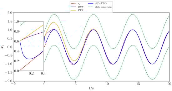
Figure 1. Trajectory tracking of state $x_1$ in different methods under state constraints.

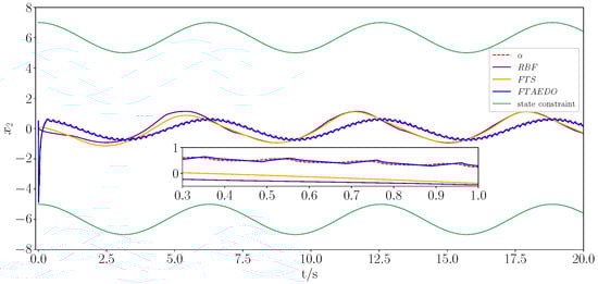
Figure 2. Trajectory tracking of state $x_2$ in different methods under state constraints.

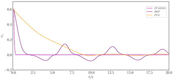
Figure 3. Trajectory tracking of the error $e_1$ under different methods.

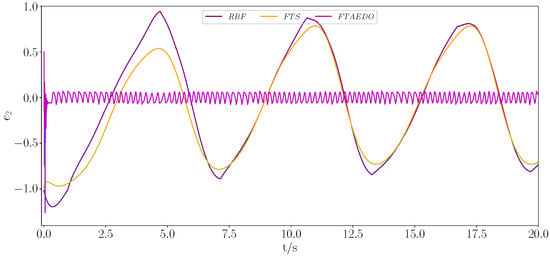
Figure 4. Trajectory tracking of the error $e_2$ under different methods.

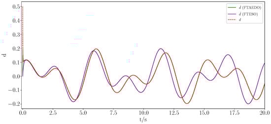
Figure 5. Observation curves of unknown disturbances under different methods.

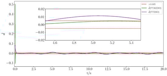
Figure 6. Observation error curves of unknown disturbances under different methods.

The simulation results are presented in Figure 1, Figure 2, Figure 3, Figure 4, Figure 5, Figure 6, Figure 7 and Figure 8. Figure 1 and Figure 2 show the trajectory tracking of states $x_1$ and $x_2$ under the constraints using different methods, while Figure 3 and Figure 4 demonstrate the tracking errors $e_1$ and $e_2$ for different methods, respectively. The figures clearly show that the proposed method outperformed both the RBFNN and FTS in terms of the convergence speed and tracking accuracy. While the RBFNN-based approach suffered from slow convergence due to its reliance on iterative learning, the FTS-based method, despite ensuring finite-time stability, failed to achieve rapid convergence and effective error reduction. In contrast, the proposed method consistently maintained a smooth and stable tracking performance throughout the simulation, achieving faster convergence and significantly lower tracking errors. Figure 5 and Figure 6 depict the observation of positional perturbations by the observer and its performance regarding its errors. Figure 7 demonstrates the variations in the control input signals, and Figure 8 illustrates the time intervals of the event triggers.

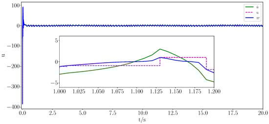
Figure 7. Control input signal.

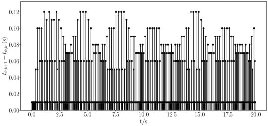
Figure 8. Event trigger interval.

From Figure 1, Figure 2, Figure 3, Figure 4, Figure 5, Figure 6, Figure 7 and Figure 8, it is evident that all signals were bounded. From Figure 1 and Figure 3, it is clear that the actual trajectory of $x_1$ tracked the expected trajectory well, and its error could be stabilized within 0.5%, indicating that the proposed control method can guarantee excellent tracking performance. From Figure 2 and Figure 4, it is evident that the actual trajectory of $x_2$ tracked the expected trajectory well, even under constraints. The estimation of the positional perturbation by the observer is clearly demonstrated in Figure 5, and in Figure 6, it is shown that the observer reached a steady state by 0.2 s and the error was maintained within a 0.5% error band, reflecting the excellent performance of the designed FTDO. Figure 7 presents the control input signals, indicating that the control signals were accurate and remained within the bounded range after the system stabilized. Figure 8 presents the event-triggering interval graph, showing that the total number of triggers for the adaptive event-triggering mechanism (AETM) and Time-Triggering Mechanism (TTM) was 715 and 2000, respectively (with a fixed simulation step of 0.01 s), implying a saving of 64.25% of the communication resources. Notably, as seen in Figure 8, there was no Zeno phenomenon. In conclusion, this part of the simulation demonstrated the effectiveness of the proposed control method.

4.2. Example Simulation of Single-Link Robotic Arm System

In order to verify the effectiveness of the control method designed above in a real system, the following single-link robotic arm system was considered:

$$J\ddot{q}+B\dot{q}+mglsin\left(q\right)=u+d$$

(71)

where $x_1=q$ and $x_2=\dot{q}$ denote the joint angles and angular velocities, respectively, u denotes the input torque, and d is the unknown perturbation. Then, the system can be rewritten as

$$\left\{\begin{array}{c}{\dot{x}}_1\left(t\right)=x_2\hfill \\ {\dot{x}}_2\left(t\right)=-{\displaystyle \frac{mglsin\left(x_1\right)+B{x}_2}{J}}+{\displaystyle \frac{u+d}{J}}\hfill \end{array}\right.$$

(72)

The parameters of the robotic arm system were $J=0.5$, $B=1$, and $mgl=9.8$; the parameter design was the same as the numerical simulation parameter design except for the initial state of $x_1\left(0\right)=0.5$ for $x_1$.

Figure 9, Figure 10, Figure 11, Figure 12, Figure 13, Figure 14, Figure 15 and Figure 16 show the simulation results for the single-link robotic arm system, which was analysed similarly to the numerical simulation. By utilizing the above control method, the desired tracking performance and the boundedness of all the signals were guaranteed, and the predefined constraint intervals were not violated. In addition, it was guaranteed that the Zeno phenomenon would not occur.

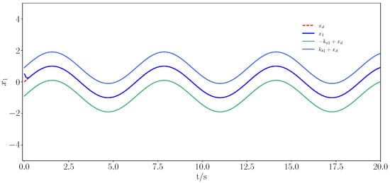
Figure 9. Trajectory tracking under constraints for state $x_1$.

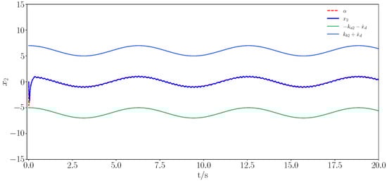
Figure 10. Trajectory tracking under constraints for state $x_2$.

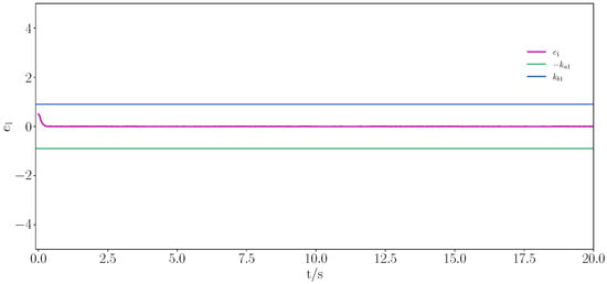
Figure 11. Trajectory tracking under constraints for error $e_1$.

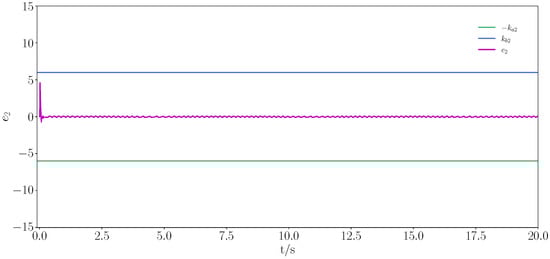
Figure 12. Trajectory tracking under constraints for error $e_2$.

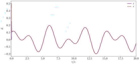
Figure 13. Unknown disturbance observation curve.

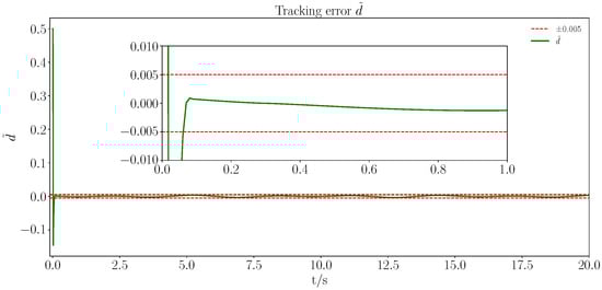
Figure 14. Unknown disturbance observation error curve.

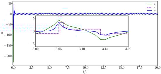
Figure 15. Control input signal.

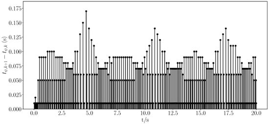
Figure 16. Event trigger interval.

5. Conclusions

In this paper, the fixed-time control problem for uncertain nonlinear systems with full-state constraints and unknown time-varying external perturbations was investigated. Using adaptive parameters, an adaptive event-triggering mechanism scheme was proposed to save communication resources. In addition, a fixed-time disturbance observer was designed to compensate for the effects of external disturbances. Using the proposed method, the system could be stabilised in a fixed time with arbitrary initial conditions. This was verified using examples given in the Simulation Section. In future work, we will focus on how to achieve the stable control of the system at a predefined time while examining the performance of the system and investigating the proposed method to achieve stability under conditions with time-varying constraints.

References

- Liu, S.; Zuo, Y.; Li, T.; Wang, H.; Gao, X.; Xiao, Y. Adaptive fixed-time PID-based control of uncertain nonlinear systems and its application to unmanned surface vehicles. Int. J. Syst. Sci. 2024, 55, 2815–2824. [Google Scholar] [CrossRef]
- Pi, W.; Liu, W. Event-triggered finite-time neural control for uncertain nonlinear systems with unknown disturbances and its application in SVC. Trans. Inst. Meas. Control 2024, 46, 1803–1814. [Google Scholar] [CrossRef]
- Han, H.G.; Feng, C.C.; Sun, H.Y.; Qiao, J.F. Hierarchical Self-Organizing Fuzzy Control for Uncertain Nonlinear Systems. IEEE Trans. Fuzzy Syst. 2024, 32, 2471–2482. [Google Scholar] [CrossRef]
- Lü, S.; Shen, H. Adaptive Fuzzy Asymptotic Tracking Control of Uncertain Nonlinear Systems with Full State Constraints. IEEE Trans. Fuzzy Syst. 2024, 32, 2750–2761. [Google Scholar] [CrossRef]
- Sun, Z.; Hua, C. Logic-Based Fixed-Time Control for Uncertain Nonlinear Systems with Unknown Control Directions. IEEE Trans. Cybern. 2024, 54, 5337–5346. [Google Scholar] [CrossRef] [PubMed]
- Huang, G.; Zhao, X.; Zhao, B.; Han, L.; Yu, P. Disturbance Rejection Approach for Nonlinear Systems Using Kalman-Filter-Based Equivalent-Input-Disturbance Estimator. Actuators 2025, 14, 189. [Google Scholar] [CrossRef]
- Gao, X.; Li, X.; Xiao, J.; Hao, L. Robust PI-Type Output Feedback Control of Unknown Nonlinear Systems. IEEE Trans. Ind. Electron. 2022, 69, 9396–9405. [Google Scholar] [CrossRef]
- Greene, M.L.; Bell, Z.I.; Nivison, S.; Dixon, W.E. Deep Neural Network-Based Approximate Optimal Tracking for Unknown Nonlinear Systems. IEEE Trans. Autom. Control 2023, 68, 3171–3177. [Google Scholar] [CrossRef]
- Shen, X.; Liu, G.; Liu, J.; Gao, Y.; Leon, J.I.; Wu, L.; Franquelo, L.G. Fixed-Time Sliding Mode Control for NPC Converters with Improved Disturbance Rejection Performance. IEEE Trans. Ind. Inform. 2025, 1–12. [Google Scholar] [CrossRef]
- Wang, Z.; Guo, Z.; Li, S. Finite-Time Disturbance Rejection Control for Rigid Spacecraft Attitude Set Stabilization with Actuator Saturation. IEEE Trans. Aerosp. Electron. Syst. 2024, 60, 4910–4922. [Google Scholar] [CrossRef]
- Polyakov, A. Nonlinear Feedback Design for Fixed-Time Stabilization of Linear Control Systems. IEEE Trans. Autom. Control 2012, 57, 2106–2110. [Google Scholar] [CrossRef]
- Wei, Y.; Xie, C.; Zhang, X.; Xu, Y. Finite/Fixed-Time Synchronization for Stochastic Multilayer Networks with Pinning Control. IEEE Access 2024, 12, 79667–79674. [Google Scholar] [CrossRef]
- Cui, L.; Jin, N.; Chang, S.; Zuo, Z.; Zhao, Z. Fixed-time ESO based fixed-time integral terminal sliding mode controller design for a missile. ISA Trans. 2022, 125, 237–251. [Google Scholar] [CrossRef]
- Zhang, Y.; Pang, K.; Zhou, J.; Yang, Y.; Hua, C. Fixed-Time Composite Learning Control of Robots with Prescribed Time Error Constraints. IEEE/ASME Trans. Mechatronics 2024, 30, 426–435. [Google Scholar] [CrossRef]
- Mi, Z.; Kong, Z.; Huang, T.; Shi, P.; Yu, Z.; Ding, L. Fixed-Time Hierarchical Distributed Control for Flexible Thermostatically Controlled Loads. IEEE Syst. J. 2024, 18, 1344–1355. [Google Scholar] [CrossRef]
- Cao, L.; Xiao, B.; Golestani, M.; Ran, D. Faster Fixed-Time Control of Flexible Spacecraft Attitude Stabilization. IEEE Trans. Ind. Inform. 2020, 16, 1281–1290. [Google Scholar] [CrossRef]
- Li, L.J.; Chang, X.; Chao, F.; Lin, C.M.; Huỳnh, T.T.; Yang, L.; Shang, C.; Shen, Q. Self-Organizing Type-2 Fuzzy Double Loop Recurrent Neural Network for Uncertain Nonlinear System Control. IEEE Trans. Neural Netw. Learn. Syst. 2024, 36, 6451–6465. [Google Scholar] [CrossRef]
- Qian, W.; Wu, Y.; Shen, B. Novel Adaptive Memory Event-Triggered-Based Fuzzy Robust Control for Nonlinear Networked Systems via the Differential Evolution Algorithm. IEEE/CAA J. Autom. Sin. 2024, 11, 1836–1848. [Google Scholar] [CrossRef]
- Khan, G.D. Adaptive Neural Network Control Framework for Industrial Robot Manipulators. IEEE Access 2024, 12, 63477–63483. [Google Scholar] [CrossRef]
- Wei, M.; Zheng, L.; Li, H.; Cheng, H. Adaptive Neural Network-Based Model Path-Following Contouring Control for Quadrotor Under Diversely Uncertain Disturbances. IEEE Robot. Autom. Lett. 2024, 9, 3751–3758. [Google Scholar] [CrossRef]
- Gao, N.; Tang, J.; Lin, J.; Sheng, G.; Chen, H. Nonlinear Dynamic Observer Design for Uncertain Vehicle Systems with Disturbances. IEEE Access 2024, 12, 48394–48403. [Google Scholar] [CrossRef]
- Nurminen, T.; Mourouvin, R.; Hinkkanen, M.; Kukkola, J. Multifunctional Grid-Forming Converter Control Based on a Disturbance Observer. IEEE Trans. Power Electron. 2024, 39, 13023–13032. [Google Scholar] [CrossRef]
- Zhang, Z.; Wang, Q.; Sang, Y.; Ge, S.S. Globally Adaptive Neural Network Output-Feedback Control for Uncertain Nonlinear Systems. IEEE Trans. Neural Netw. Learn. Syst. 2023, 34, 9078–9087. [Google Scholar] [CrossRef]
- Hou, Q.; Ding, S. Finite-Time Extended State Observer-Based Super-Twisting Sliding Mode Controller for PMSM Drives with Inertia Identification. IEEE Trans. Transp. Electrif. 2022, 8, 1918–1929. [Google Scholar] [CrossRef]
- Li, S.; Wang, Y.; Tan, J.; Zheng, Y. Adaptive RBFNNs/integral sliding mode control for a quadrotor aircraft. Neurocomputing 2016, 216, 126–134. [Google Scholar] [CrossRef]
- Liu, Z.; Zhao, Y.; Zhang, O.; Chen, W.; Wang, J.; Gao, Y.; Liu, J. A Novel Faster Fixed-Time Adaptive Control for Robotic Systems with Input Saturation. IEEE Trans. Ind. Electron. 2024, 71, 5215–5223. [Google Scholar] [CrossRef]
- Zhou, Z.; Shen, Y.; Chen, M. Finite-Time Control for Maneuvering Aircraft with Input Constraints and Disturbances. Actuators 2025, 14, 194. [Google Scholar] [CrossRef]
- Wang, J.; Li, Y.; Wu, Y.; Liu, Z.; Chen, K.; Chen, C.L.P. Fixed-Time Formation Control for Uncertain Nonlinear Multiagent Systems with Time-Varying Actuator Failures. IEEE Trans. Fuzzy Syst. 2024, 32, 1965–1977. [Google Scholar] [CrossRef]
- Liu, Z.; Liu, J.; Zhang, O.; Zhao, Y.; Chen, W.; Gao, Y. Adaptive Disturbance Observer-Based Fixed-Time Tracking Control for Uncertain Robotic Systems. IEEE Trans. Ind. Electron. 2024, 71, 14823–14831. [Google Scholar] [CrossRef]
- Chen, H.; Zong, G.; Zhao, X. Asynchronous Secure Control of Fuzzy MJSs with Time Delays: A Multi-Level Probabilistic Event-Triggered Mechanism. IEEE Trans. Autom. Sci. Eng. 2024, 22, 5436–5447. [Google Scholar] [CrossRef]
- He, J.; Liao, J. Formation tracking control with disturbance rejection in leader-follower multi-agent systems under dynamic event-triggered mechanism. Eng. Appl. Artif. Intell. 2024, 133, 108441. [Google Scholar] [CrossRef]
- Wang, Y.; Sun, Y.; Zhang, Y.; Huang, J. Predefined-Time Adaptive Neural Tracking Control for a Single Link Manipulator with an Event-Triggered Mechanism. Sensors 2024, 24, 4573. [Google Scholar] [CrossRef] [PubMed]
- Hao, P.W.; Feng, G.C.; Li, J.W. Leader-Follower Formation Tracking Control and Stabilization of Underactuated Unmanned Surface Vessels via Event-Triggered Mechanism. IEEE Access 2024, 12, 80359–80372. [Google Scholar] [CrossRef]
- Yuan, Y.; He, W.; Du, W.; Tian, Y.C.; Han, Q.L.; Qian, F. Distributed Gradient Tracking for Differentially Private Multi-Agent Optimization with a Dynamic Event-Triggered Mechanism. IEEE Trans. Syst. Man, Cybern. Syst. 2024, 54, 3044–3055. [Google Scholar] [CrossRef]
- Zhang, X.M.; Han, Q.L.; Zhang, B.L.; Ge, X.; Zhang, D. Accumulated-state-error-based event-triggered sampling scheme and its application to H∞ control of sampled-data systems. Sci. China Inf. Sci. 2024, 67, 162206. [Google Scholar] [CrossRef]
- Xiao, C.; Tang, L.; Wang, F.; You, S.; Xu, H.; Chen, M.; Lu, Z. Event-Triggered Control for Flapping-Wing Robot Aircraft System Based on High-Gain Observers. Actuators 2025, 14, 190. [Google Scholar] [CrossRef]
- Zhou, T.; Zuo, Z.; Wang, Y. Self-Triggered and Event-Triggered Control for Linear Systems with Quantization. IEEE Trans. Syst. Man, Cybern. Syst. 2020, 50, 3136–3144. [Google Scholar] [CrossRef]
- Zhang, X.M.; Han, Q.L.; Ge, X.; Zhang, B.L. Accumulative-Error-Based Event-Triggered Control for Discrete-Time Linear Systems: A Discrete-Time Looped Functional Method. IEEE/CAA J. Autom. Sin. 2025, 12, 683–693. [Google Scholar] [CrossRef]
- Wang, J.; Zhang, H.; Ma, K.; Liu, Z.; Chen, C.L.P. Neural Adaptive Self-Triggered Control for Uncertain Nonlinear Systems with Input Hysteresis. IEEE Trans. Neural Netw. Learn. Syst. 2022, 33, 6206–6214. [Google Scholar] [CrossRef]
- Hu, X.; Li, Y.X.; Hou, Z. Event-Triggered Fuzzy Adaptive Fixed-Time Tracking Control for Nonlinear Systems. IEEE Trans. Cybern. 2022, 52, 7206–7217. [Google Scholar] [CrossRef]
- Tee, K.P.; Ge, S.S.; Li, H.; Ren, B. Control of Nonlinear Systems with Time-Varying Output Constraints. In Proceedings of the IEEE International Conference on Control & Automation, Christchurch, New Zealand, 9–11 December 2009. [Google Scholar]
- Li, Y.X.; Hu, X.; Che, W.; Hou, Z. Event-Based Adaptive Fuzzy Asymptotic Tracking Control of Uncertain Nonlinear Systems. IEEE Trans. Fuzzy Syst. 2021, 29, 3003–3013. [Google Scholar] [CrossRef]
Disclaimer/Publisher’s Note: The statements, opinions and data contained in all publications are solely those of the individual author(s) and contributor(s) and not of MDPI and/or the editor(s). MDPI and/or the editor(s) disclaim responsibility for any injury to people or property resulting from any ideas, methods, instructions or products referred to in the content. |
© 2025 by the authors. Licensee MDPI, Basel, Switzerland. This article is an open access article distributed under the terms and conditions of the Creative Commons Attribution (CC BY) license (https://creativecommons.org/licenses/by/4.0/).