Article

Fault Diagnosis of Rolling Element Bearing Based on BiTCN-Attention and OCSSA Mechanism

1
School of Mechatronics Engineering, Qiqihar University, Qiqihar 161006, China
2
Department of Control Science and Engineering, Harbin Institute of Technology, Harbin 150001, China
3
School of Science, Qiqihar University, Qiqihar 161006, China
4
School of Electrical and Information Engineering, North Minzu University, Yinchuan 750030, China
*
Author to whom correspondence should be addressed.
Actuators 2025, 14(5), 218; https://doi.org/10.3390/act14050218
Submission received: 27 February 2025 / Revised: 1 April 2025 / Accepted: 25 April 2025 / Published: 28 April 2025
(This article belongs to the Special Issue Intelligent Sensing, Control and Actuation in Networked Systems)

Abstract

:
This paper proposes a novel fault diagnosis framework that integrates the Osprey–Cauchy–Sparrow Search Algorithm (OCSSA) optimized Variational Mode Decomposition (VMD) with a Bidirectional Temporal Convolutional Network-Attention mechanism (BiTCN-Attention). To address the limitations of empirical parameter selection in VMD, OCSSA adaptively optimizes the decomposition parameters (penalty factor α and mode number K) through a hybrid strategy that combines chaotic initialization, Osprey-inspired global search, and Cauchy mutation. Subsequently, the BiTCN captures bidirectional temporal dependencies from vibration signals, while the attention mechanism dynamically filters critical fault features, constructing an end-to-end diagnostic model. Experiments on the CWRU dataset demonstrate that the proposed method achieves an average accuracy of 99.44% across 10 fault categories, outperforming state-of-the-art models (e.g., VMD-TCN: 97.5%, CNN-BiLSTM: 84.72%).

1. Introduction

The rapid evolution of industrial automation and intelligent manufacturing has significantly raised the performance standards for fault detection and diagnosis in rotating machinery [1]. As vital transmission components in electromechanical systems, rolling element bearings have a direct impact on equipment reliability and operational integrity [2]. Severe bearing failures can trigger complete system breakdowns, resulting in operational disruptions and considerable economic losses, and safety hazards [3]. This imperative has propelled the development of sophisticated bearing fault diagnostic methodologies to the forefront of contemporary engineering research, constituting a shared priority across academic inquiry and industrial practice [4].
Vibration signal-based diagnostic methodologies for rolling element bearing failures have emerged as one of the most prevalent diagnostic modalities in industrial applications, owing to their non-invasive nature and operational efficiency. Vibration signatures provide essential health indicators of bearing operational states, making them especially useful for diagnosing incipient failure problems [5]. Consequently, the dual challenge of extracting discriminative fault features from intricate vibrational waveforms and achieving precise diagnostic interpretation constitutes a pivotal research frontier in fault detection [6]. Although vibration signal-based fault diagnosis methods have been widely adopted, existing techniques still face the following challenges: (1) Inadequate handling of non-stationary signals: traditional methods (e.g., FFT, Wavelet Transform) rely on stationarity assumptions, failing to decompose non-stationary vibration signals under real-world conditions effectively; (2) Parameter sensitivity: advanced decomposition methods (e.g., VMD) heavily depend on empirical parameter settings (mode number K, penalty factor α ), leading to unstable decomposition results; (3) Limitations in temporal modeling: existing deep learning models (e.g., LSTM, TCN) inadequately capture bidirectional temporal dependencies, restricting the diagnosis accuracy for weak faults under complex operating conditions.
Traditional vibration signal-processing methods primarily rely on frequency-domain or time–frequency analysis tools [7]. Wavelet Transform (WT), Empirical Mode Decomposition (EMD), Short-Time Fourier Transform (STFT), and Fast Fourier Transform (FFT) are popular feature-extraction methods. These methods analyze the frequency components or time–frequency characteristics of vibration signals to extract critical fault-related information. For instance, Atoui et al. (2013) investigated the application of FFT and WT in rotating machinery imbalance fault detection. They highlighted FFT’s efficiency in extracting frequency-domain components but noted its limitations in analyzing non-stationary signals. By adding time frames, STFT increases the resolution of short-time signals; nevertheless, there is a trade-off between frequency and time resolution [8]. Rai and Upadhyay (2016) examined signal-processing strategies for detecting rolling bearing faults, emphasizing WT’s flexibility in handling complex and non-stationary signals and enabling multi-scale analysis. In contrast, EMD adaptively decomposes signals and is appropriate for extracting features from complex and non-stationary signals, yet this method is subject to end effects [9]. Li, DY et al. propose a novel adaptive fault detection framework that synergizes STFT enhanced stationary feature extraction with dynamic model updating, effectively addressing non-stationary signal masking and training-test distribution discrepancies in wind turbines [10]. Wu and Qu (2009) investigated the use of EMD in subharmonic fault diagnostics for big rotating machinery. By decomposing complex vibration signals using EMD and integrating time–frequency analysis, they effectively captured underlying fault characteristics [11]. Shifat and Hur (2020) introduced a model combining Ensemble Empirical Mode Decomposition (EEMD) with supervised learning for fault diagnosis in brushless DC motors. EEMD reduces mode mixing and enhances the stability of Intrinsic Mode Functions (IMFs), resulting in more robust signal processing [12]. But many of these documents use trial and error methods to determine VMD parameters, lacking adaptive optimization mechanisms.
Despite the significant success of these classic methods in practical applications, their efficacy frequently depends on the proficiency of seasoned specialists for signal analysis and feature extraction. Furthermore, these approaches exhibit inherent limitations when dealing with complex, non-stationary, and nonlinear signals. For example, whereas FFT is ideally suited for frequency-domain analysis of stationary signals, its capability for deriving fault features from non-stationary data is constrained. Both STFT and WT, while capable of processing non-stationary signals, are hampered by a fixed time–frequency resolution, potentially resulting in the loss of vital fault-related information. Dragomiretskiy et al. devised VMD to tackle these issues [13]. This technique adaptively decomposes intricate signals into a collection of IMFs, facilitating the extraction of more accurate fault characteristics without sacrificing time–frequency resolution. VMD demonstrates significant advantages in processing non-stationary signals; however, its diagnostic performance is highly sensitive to the selection of decomposition parameters. Consequently, optimizing VMD parameters has become a critical focus of research.
In the past few years, with the quick growth of deep learning technology, data-driven fault diagnosis methods have acquired substantial interest [14]. These approaches harness the excellent feature-extraction skills of deep learning models to eliminate the dependency on manual expertise and past knowledge inherent in traditional signal-processing methods. Among these, Convolutional Neural Networks (CNNs) have emerged as a widely adopted deep learning model, capable of automatically extracting local features from signals through convolutional operations. In a study by Q. Shen and Z. Zhang, a network architecture combining multi-scale convolution and residual connections was proposed to enhance the deep learning capabilities for bearing fault diagnosis. The multi-scale convolution design enables the model to properly collect characteristics at many sizes, while the residual connections ease the vanishing gradient problem in deep networks, enhancing both learning efficiency and diagnostic performance [15]. Wen et al. introduced an innovative LeNet-5-adapted convolutional neural network with automated signal-to-image conversion capability, which innovates a novel spatiotemporal transformation mechanism that systematically encodes 1-D vibration signals into diagnosable 2-D texture representations, enabling end-to-end feature learning while obviating manual feature engineering in rotating machinery fault diagnosis [16]. Ding et al. developed an intelligent fault identification framework employing enhanced CEEMDAN coupled with distance evaluation-driven feature distillation, which creates a novel dual-stage feature refinement strategy that performs multi-scale decomposition of rolling bearing vibration signals into optimized IMFs while autonomously distilling salient fault signatures through adaptive resonance component selection [17].
Although previous studies have attempted to combine signal decomposition with deep learning, there are still significant gaps: (1) lack of parameter optimization—most literature uses trial and error methods to determine VMD parameters, lacking adaptive optimization mechanisms, resulting in decomposition quality limited by expert experience (such as literature [8]); (2) insufficient feature fusion—existing models (such as VMD-CNN-LSTM) do not fully utilize the decomposed multi-scale features and lack dynamic feature-filtering mechanisms.
Beyond CNNs, Recurrent Neural Networks (RNNs), particularly Long Short-Term Memory (LSTM) networks, have shown an extraordinary ability to process sequential signals. LSTMs are adept at capturing long-term dependencies within signals, making them widely applicable for time-series fault diagnosis. Chen et al. proposed an LSTM-based bearing fault diagnosis method that leverages CNNs for extracting local spatial features while utilizing LSTMs to capture temporal information, significantly enhancing diagnostic accuracy and robustness [18]. Pan et al. pioneered a hybrid deep diagnostic architecture featuring hierarchical CNN-LSTM integration with spatiotemporal feature fusion, which innovatively establishes an adaptive multisc [19]. Khorram et al. devised an end-to-end CNN-LSTM system that combines the feature collection skills of CNNs with the timing analysis capabilities of LSTMs, hence boosting fault diagnosis precision [20].
Over the past few years, following the advancements in RNNs, TCNs have emerged as a pivotal tool for processing time-series data. TCNs, a network architecture based on one-dimensional convolutions, employ causal and dilated convolutions to capture dependencies that endure within time-series data successfully. Unlike LSTMs, TCNs significantly enhance training efficiency through parallel computation while maintaining robust modeling capabilities for long-sequence dependencies. In the realm of fault diagnosis, TCNs have demonstrated exceptional performance. Their advantage lies in the ability to extract complex temporal patterns with relatively shallow network depths, a feat achieved through the expanded receptive fields enabled by dilated convolutions. Research indicates that, compared to LSTMs, TCNs not only reduce training time when handling high-dimensional temporal features but also exhibit more stable convergence. In certain tasks, TCNs further improve classification and prediction accuracy by mitigating the vanishing gradient problem. Additionally, the structural flexibility of TCNs makes them well suited for integration with other methodologies. For instance, Yan et al. provided a TCN-based time-series autoencoder for unsupervised anomaly detection, which significantly enhances the receptive field through dilated convolutions, effectively addressing challenges in long-sequence modeling [21]. Song et al. utilized a distributed attention approach paired with TCNs for RUL prediction, demonstrating outstanding performance in mechanical equipment health monitoring [22]. Shang et al. pioneered WD-ARCATCN an adaptive residual temporal convolutional network with broad primary-layer kernel configuration and cross-sensor feature amalgamation, establishing the first vibration signal cross-modal representation framework [23]. Xing et al. developed TCB-CNN, a temporal convolutional block network with a dual-path temporal learning architecture that fundamentally advanced time-series modeling [24]. Huang et al. proposed an ensemble learning method based on Complete Ensemble Empirical Mode Decomposition with Adaptive Noises (CEEMDAN) and deep temporal convolutional network (DeepTCN) for short-term photovoltaic power generation prediction [25].
Despite the remarkable achievements of existing deep learning methods in bearing fault diagnosis, these approaches often exhibit limitations in feature extraction and temporal information capture. For example, while CNNs excel at local feature extraction, they fall short in temporal modeling. Conversely, LSTMs, though proficient in handling sequential data, are less effective in local feature extraction compared to CNNs. As a result, a significant research topic includes combining CNNs’ local feature extraction skills with LSTMs’ temporal modeling powers to create an end-to-end unified fault diagnostic model.
To overcome these difficulties, this research provides a novel bearing failure detection approach that combines VMD enhanced by the OCSSA with a BiTCN-Attention. By optimizing VMD decomposition parameters using OCSSA, complex vibration signals can be more precisely decomposed, enabling the extraction of fault features across different frequency components. Subsequently, the BiTCN model extracts features from both past and future time steps of the vibration signal, while the attention mechanism focuses on key information, hence boosting diagnostic accuracy. Experimental validation reveals the efficacy of this method in rolling bearing failure diagnosis, with results suggesting strong diagnostic performance and generalization capabilities across varied operational situations.
The rest of this paper is arranged as follows: Section 2 elaborates on the OCSSA-VMD algorithm for optimized signal decomposition. Section 3 details the BiTCN-Attention prediction model. Section 4 presents experimental validation and comparative analysis using the CWRU dataset. The conclusions are given in Section 5.

2. Bearing Data Decomposition Based on OCSSA-VMD

2.1. Osprey–Cauchy–Sparrow Search Algorithm

The hunting behavior of sparrow populations naturally inspires an optimization process, which led to the development of the Sparrow Search Algorithm (SSA) [26]. The SSA demonstrates commendable stability and rapid convergence, offering a balanced ability for both global exploration and local exploitation. However, its reliance on the previous generation’s position update mechanism often results in an over-dependence on historical data and an increased risk of converging to local optima. To solve these limitations, we present an upgraded Sparrow Search Algorithm coupled with Osprey optimization and Cauchy mutation, incorporating the following three improvements:
(1) To boost the diversity of the starting population, logistic chaotic mapping is applied to achieve a uniform distribution of initial solutions over the solution space. The mathematical formulation is as follows:
x k + 1 = μ x k ( 1 x k )
where x k ( 0 , 1 ] represents a random number, and μ ( 0 , 4 ] denotes a tunable parameter. The term x k + 1 corresponds to the mapping function of x k . In this study, μ is set to 3.98 to ensure a uniform distribution of the initial sequence.
(2) The Osprey Optimization Algorithm (OOA) [27] is utilized to substitute the position update formula for the explorers in the original Sparrow Search Algorithm (SSA) during the early phase of global exploration. This integration addresses the SSA’s over-reliance on the position update mechanism of the previous generation. The OOA mimics the hunting behavior of ospreys, where a random prey position is identified and targeted. By simulating the osprey’s movement toward its prey, the position update mechanism for the explorers in the SSA is enhanced, thereby improving global exploration capabilities.
(3) The Cauchy mutation approach [28] is utilized to substitute the position update formula for the followers in the original SSA. The Cauchy distribution, a continuous probability distribution, generates larger perturbations compared to the Gaussian distribution, making it more effective in diversifying the population. Cauchy mutation is employed to broaden the search scope and avert the algorithm from converging to local optima by perturbing the positions of individuals throughout the update phase. The updated position of the sparrows is formulated as follows:
X i , j k + 1 = X best ( k ) + Cauchy ( 0 , 1 ) X best ( k )
where Cauchy (0, 1) signifies the usual Cauchy distribution function, and ⊕ indicates the multiplication operation.

2.2. Variational Mode Decomposition

The core principle of Variational Mode Decomposition (VMD) is that any signal can be regarded as a composition of sub-signals, each represented by a distinct Intrinsic Mode Function (IMF). VMD employs an iterative strategy to optimize the variational model. This methodology enables the precise estimation of each component’s center frequency and bandwidth, effectively mitigating issues such as endpoint effects and mode mixing. The primary objective of the VMD method is to ensure, through appropriate parameter configuration, that the deconstructed modal components are unaffected by frequency aliasing and can accurately recover the original frequency components. In VMD, each IMF is mathematically defined as an amplitude-modulated and frequency-modulated function:
u k ( t ) = A k ( t ) cos ϕ k ( t )
where the amplitude–frequency modulated signal u k ( t ) is the IMF component, A k ( t ) is the instantaneous amplitude, φ k ( t ) is the instantaneous phase.
To construct the limited variational model and determine each mode component’s frequency:
(1) The Hilbert transform is applied to each modal function u k ( t ) to derive its analytic signal:
δ ( t ) + j π t * u k ( t )
(2) Each fundamental frequency band is modulated via frequency shifting to align with the corresponding spectral components of the modal functions:
δ ( t ) + j π t * u k ( t ) * e j w t
(3) The restricted variational model is applied to estimate and demodulate the bandwidth of each modal function by Gaussian smoothing:
min u , w k t δ ( t ) + j π t * u k ( t ) * e j w t 2
s . t . k = 1 K u k ( t ) = f ( t )
where t denotes the partial derivative of a function with respect to time, f ( t ) represents the input signal, δ ( t ) is the unit impulse function, j represents the imaginary unit, and * refers for the convolution operator.
(4) Introduce penalty parameters α and Lagrange multipliers λ , and transform them into unconstrained variational problems:
L ( { u k } , { ω k } , λ ) = α k t δ ( t ) + j π t u k ( t ) e j ω k t 2 2 + f ( t ) k u k ( t ) 2 2 + λ ( t ) , f ( t ) k u k ( t )

2.3. Optimize VMD Parameters Using OCCSA

When employing the Osprey–Cauchy–Sparrow Search Algorithm (OCSSA) to optimize the penalty factor α and the number of decomposition modes K in VMD, it is crucial to define a fitness function as the evaluation metric. During each iteration, the fitness function is computed and updated until an optimal solution is achieved. The fitness function for the OCSSA, which incorporates the Osprey optimization and Cauchy mutation techniques, is chosen as follows:
(1) Minimum permutation entropy. Permutation entropy can effectively express the variety of time series, and after normalization, permutation entropy more accurately reflects the regularity of time series. The regularity of permutation entropy is directly proportional to the time series:
H ( x ) = i = 1 k p i lg ( p i ) lg ( m ! )
(2) Minimum information entropy. It describes the degree of uncertainty in system events. Due to the cyclical impact, the IMF obtained from decomposition exhibits higher orderliness in the fault information of pairs, resulting in lower entropy values:
H ( x ) = i = 1 N p i lg p i
(3) Minimum envelope spectral entropy. The envelope spectral entropy reflects the magnitude of signal envelope fluctuations and can quantitatively describe the degree of envelope differences between different signals. The lesser the entropy variety, the greater the stability of the signal, indicating a better decomposition effect of VMD:
H = f p ( f ) log p ( f )
This article combines two strategies, employing composite index permutation entropy and mutual information entropy as fitness functions, to search for the optimal decomposition level and penalty factor for each IMF component.
The optimization procedure is as follows:
Step 1: Choose the number of decomposition layers, denoted as k, with an initial value of 1, gradually increasing up to 10. After each iteration, VMD records the minimum permutation and information entropy for each mode component. Once the permutation and information entropy reach their minimum value, the corresponding amount of modes K is picked, and the iteration is terminated.
Step 2: Set the initial parameters for OCSSA and VMD, and initialize the sparrow population size.
Step 3: Based on Equations (1) and (2), find the positions of the newly added members and scouts in the population, calculate their fitness, and identify the most suitable position for the sparrow individual.
Step 4: Calculate the fitness of the optimal sparrow. If the stopping condition for the iteration is not met, return to Step 3.
Step 5: Extract the optimal IMF component for each sample using the criterion of minimizing the envelope entropy. Then, calculate the nine indicators for each component to form the feature matrix.

3. BiTCN-Attention Prediction Model

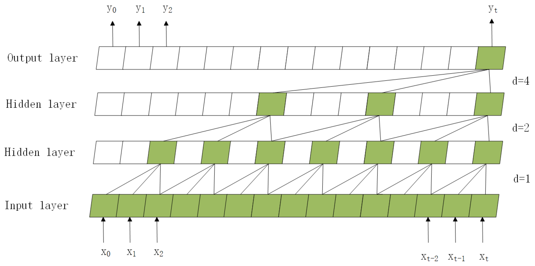
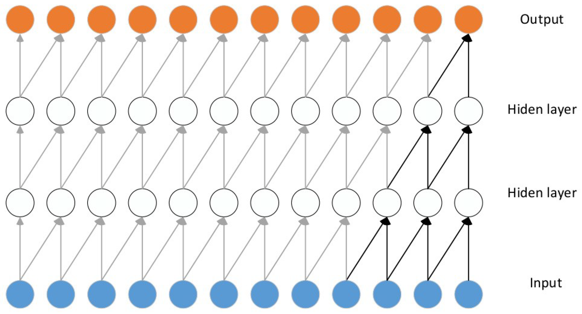
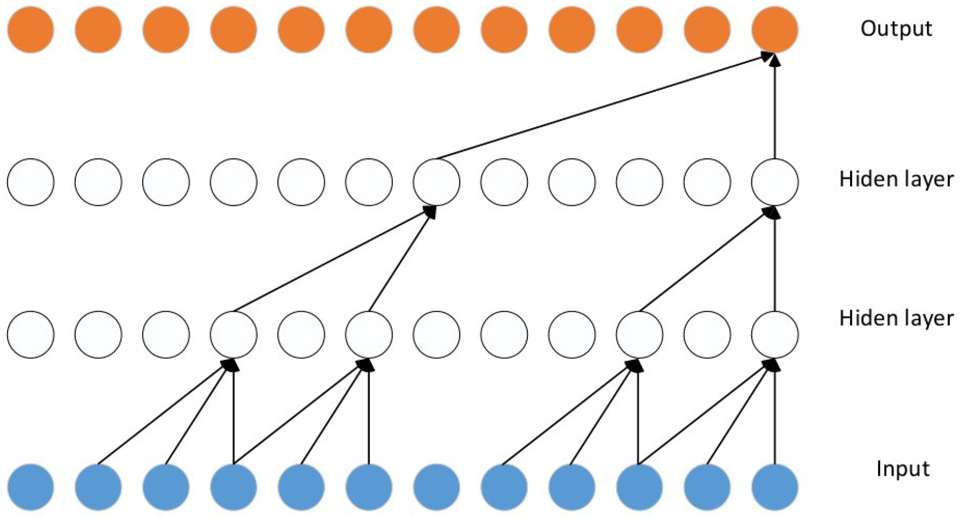
3.1. Temporal Convolutional Network

The traditional TCN comprises causal convolution, dilated convolution, and residual connections, as shown in Figure 1. Essentially, it is a one-dimensional convolution that preserves equal input and output lengths. With the introduction of dilated convolutions, TCNs achieve an enlarged receptive field without necessitating an increase in network depth. The dilation coefficients are set as [1, 2, 4], where each coefficient determines the spacing between the elements of the input sequence that are considered by the convolutional kernel. This spacing allows the network to capture dependencies over longer time intervals, effectively expanding the receptive field. The causality of causal convolution is reflected in the fact that the input sequence x = ( x 1 , x 2 , , x t ) is output as y = ( y 1 , y 2 , , y t ) after passing through the network, where the output y t at each time point depends solely on the inputs before the current time. The description of the dilated causal convolution and residual module in the TCN model is as follows:
For the input sequence x = ( x 1 , x 2 , , x t ) and the convolution kernel f : { 0 , , k 1 } R , the dilated convolution of an element s in the sequence is defined as follows:
F ( s ) = i = 0 k 1 f ( i ) · x s d · i
where s denotes the extent of the convolution kernel, reflecting the direction of the past. d is the dilation factor, which indicates the number of zero vectors inserted between adjacent convolution kernels. With each convolution layer, the dilation coefficient d increases exponentially.

3.1.1. Dilated Causal Convolution

Unlike typical convolutional neural networks, causal convolution is unable to use future data. Figure 2 illustrates a schematic of causal convolution. For the value of a neuron at time t, information can only be gathered from the present or past data at time t or earlier from the preceding layer’s neurons. For the input sequence X = ( x 1 , x 2 , , x T ) , if the convolution kernel is F = ( f 1 , f 2 , , f K ) , then the output of the causal convolution is the following:
( F * X ) ( x t ) = k = 1 K f k x t K + k
In Figure 2, each point represents a neuron. As the sequence signal is delivered from left to right, the neurons in the hidden and output layers only employ the current or previous sequence signals for calculation. Causal convolution collects features exclusively from past vibration information and is utilized for real-time diagnosis, allowing the trained model to swiftly detect defect characteristics and execute diagnosis. However, causal convolution results in a very limited receptive field, and to extract meaningful information from specific previous signals, the network must be deepened. These limitations will be addressed by other network structures.
The dilation factor is introduced in causal convolution. When connecting neurons from the previous layer, the dilated convolution layer does not fully connect; just one neuron from every several upper-layer neurons is coupled to the next layer neuron. Figure 3 illustrates a schematic of dilated convolution. For the input sequence X = ( x 1 , x 2 , , x T ) , if the convolution kernel is F = ( f 1 , f 2 , , f K ) , the output of the causal convolution is given as follows:
( F * d X ) ( x t ) = k = 1 K f k x t ( K k ) d

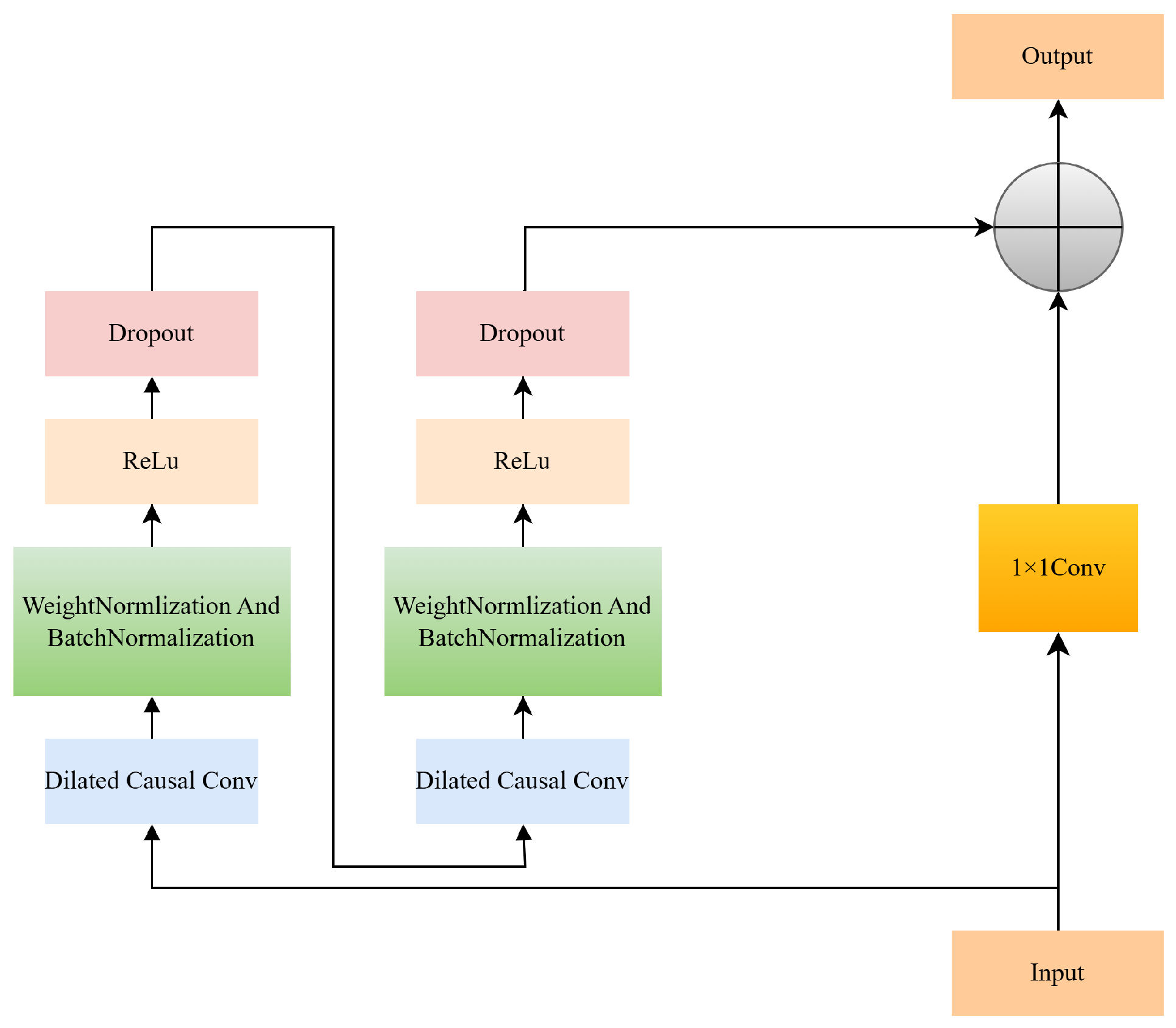
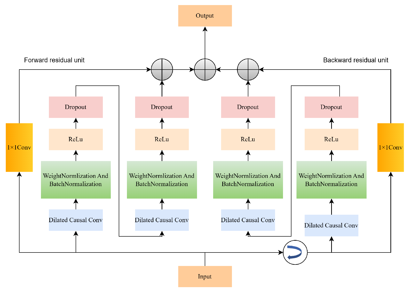
3.1.2. Residual Module

To deepen the network without encountering degradation issues during training, TCN introduces residual connections. These connections enable the input x to bypass several layers, thereby facilitating identity mapping and improving training stability. This assists the network in learning the residuals between the input and output, enhances training stability, and speeds up network convergence. Residual connections are combined with other network layers to form the residual module, ensuring that while the network depth increases, the gradient stability is maintained, and the model performance does not degrade rapidly with increased depth. The architecture of the residual module in TCN is depicted in Figure 4.
In the TCN residual block, the input data is split into two main paths. One path firstly passes through a dilated causal convolution layer, followed by weight normalization and batch normalization, then through an activation function layer and a dropout layer. The other path performs a 1 × 1 convolution operation. Finally, the outputs from both paths are added together to obtain the output of the residual module. The depth of the TCN network may be freely changed by varying the number of stacked residual blocks.
G ( x ) = f ( D ( x ) + x )
where f represents the activation function of the neural network, x signifies input data to the TCN residual module, and D is the function obtained after passing the data through a series of processing layers in the residual module.

3.2. Self-Attention Layer

The self-attention layer dynamically captures the correlations between different positions within the input data, thereby enabling global feature extraction and significantly enhancing the model’s ability to capture long-term dependencies. Its dynamic weight allocation mechanism assigns greater attention to key features while diminishing the interference of irrelevant information, thus improving the model’s diagnostic accuracy and robustness. At the same time, the self-attention layer eliminates the sequential dependencies of traditional recurrent networks, allowing parallel processing of the input sequence and greatly improving computational efficiency. Furthermore, its flexible feature-capturing ability enables it to adapt to the processing needs of complex, multidimensional signals, making it a critical component in increasing the performance of deep learning models.
Q = Q * W i Q ,
K = K * W i K ,
V = V * W i V .
where matrices Q, K, and V are composed of query vector, key vector, and value vector, respectively.
The layer receives the output H from the BiTCN network layer, as shown as follows:
Q = K = V = H .
The result is then obtained as follows:
M i = s o f t max Q K T d V .

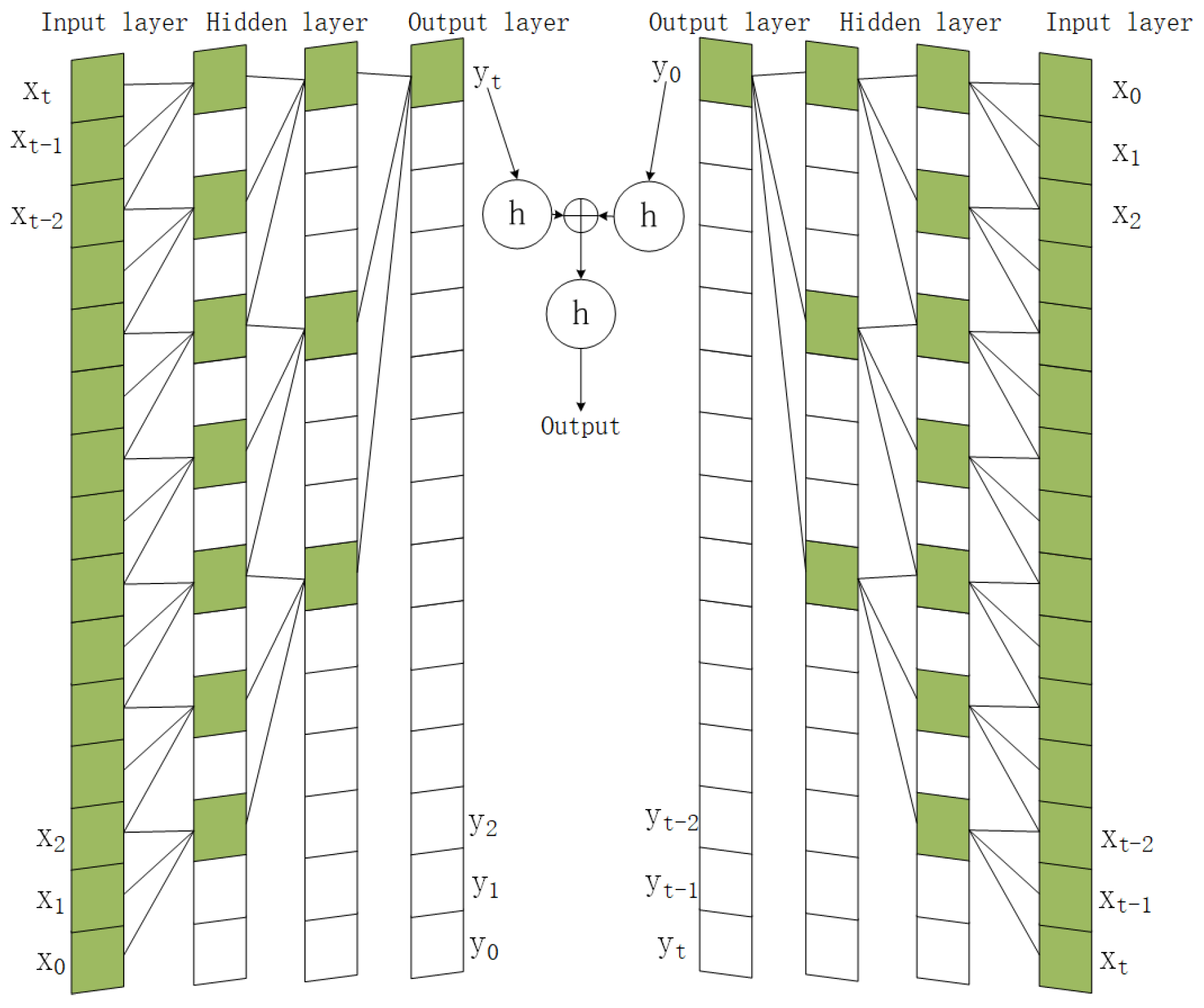
3.3. BiTCN-Attention

The conventional TCN operates unidirectionally, capturing only forward-moving data features and consequently neglecting valuable backward information. To overcome this limitation, we extend the TCN into a bidirectional form—BiTCN, thereby capturing both forward and backward temporal dependencies and fusing them to generate the final output. Furthermore, an attention mechanism is incorporated to selectively emphasize critical features, resulting in a comprehensive end-to-end diagnostic framework. The network topology of BiTCN is presented in Figure 5, and the residual block is presented in Figure 6. Two basic residual units are merged into one residual block. The forward processing of the incoming data is the responsibility of one residual block, while the backward processing is the responsibility of the other. A ReLU activation function is used after each residual block, and dropout regularization is applied to address the overfitting issue. Regarding data normalization, weight normalization is conducted on the data processed by the dilated causal convolution layer. Finally, a 1 × 1 convolution operation is added as a residual link, and the processed forward and backward data are fused to generate the final model output. The BiTCN architecture consists of two residual blocks for bidirectional temporal modeling. Each block includes dilated causal convolution with a kernel size of 3 and dilation rates of [1, 2, 4, 8], which increase exponentially across layers; weight normalization and batch normalization after convolution; and dropout (rate = 0.2) for regularization. ReLU activation is applied for nonlinear transformation. The model is trained using the Adam optimizer with a learning rate of 0.001.

4. Research Results and Analysis

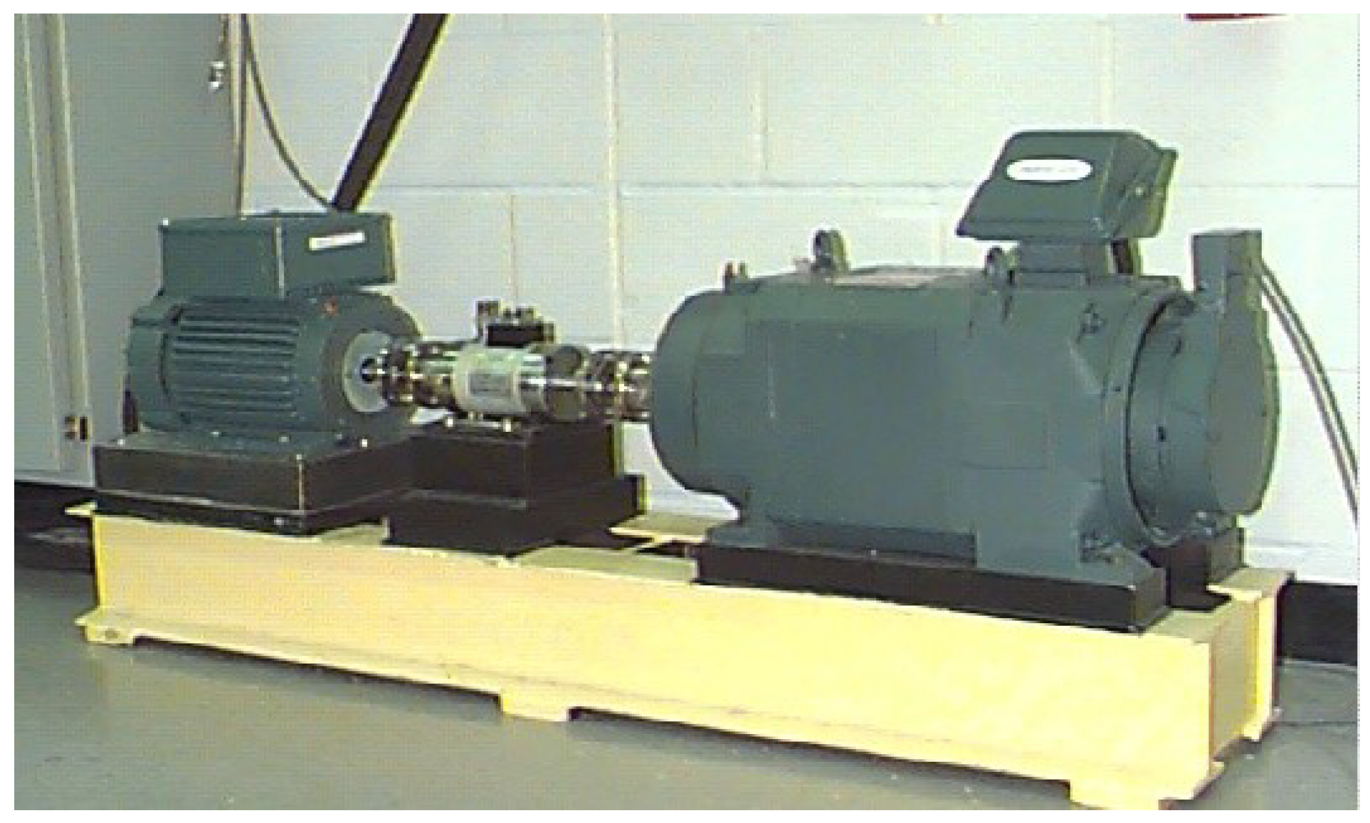
4.1. Data Source Selection

The vibration data were collected from the Case Western Reserve University (CWRU) bearing test rig [29], as shown in Figure 7. A 2-horsepower induction motor drives a shaft with a deep groove ball bearing (SKF6205) mounted on the drive end. Faults were introduced via EDM with controlled diameters (0.1778 mm, 0.3556 mm, 0.5334 mm). Accelerometers were mounted on the motor casing to gather vibration data at a sampling frequency of 12 kHz. For normal condition data, the bearings were undamaged and operated under identical mechanical configurations. Each fault type was tested under a motor load of 0 horsepower (1797 rpm), and 10-second continuous vibration signals were recorded for each condition. The raw signals were segmented into 2048-point samples using a sliding window (step size = 1024) to ensure temporal continuity and adequate sample diversity. Nonlinearity in the CWRU dataset arises from the dynamic interactions between bearing components (e.g., rolling elements, raceways) under fault conditions. Non-stationarity stems from time-varying statistical properties, and motor RPM varies slightly even under “constant” load.
The experiment establishes ten data categories, including the normal state and nine fault states based on fault diameters (0.1778 mm, 0.3556 mm, and 0.5334 mm). Each category has 120 samples, and all of them consist of 2048 data points. After feature extraction, the total sample size is 1200, divided into 840 training samples and 360 testing samples in a ratio of 70–30%. The final dataset forms a 1200 × 9 matrix, with each row containing labeled data. The labels from 1 to 10 correspond to the normal state and different fault types (such as inner race fault at 0.1778 mm, rolling element fault, outer race fault, and similar categories for 0.3556 mm and 0.5334 mm). The fault dataset partition is given in Table 1, and time-domain diagrams of some experimental vibration signals are shown in Figure 8. In this study, to perform frequency-domain analysis of the vibration signals, we applied the Fast Fourier Transform (FFT) directly on the raw signal. As a result, the obtained spectrum is the single-sided amplitude spectrum of the raw signal.
By comparing Figure 8a–d, it is evident that the change in operating conditions significantly affects the vibration characteristics. Under normal load conditions, the signal amplitude is small, and the vibration is stable with energy evenly distributed in the frequency spectrum, showing that the bearing is in optimal operating condition. Under inner race fault conditions, the time-domain signal exhibits distinct periodic impact characteristics, and the frequency-domain signal displays strong spikes at the inner race fault characteristic frequency and its harmonics, reflecting the periodic vibration enhancement caused by the inner race fault. The rolling element fault manifests as irregular impact characteristics in the time-domain signal, with a wider spectral distribution. Although the characteristic frequency spikes are still significant, the energy is more dispersed. Outer race fault results in the most intense vibration characteristics, with larger impact amplitudes and more pronounced periodicity in the time-domain signal.
Although the vibration signals for different faults are distinct, they represent idealized signals. In reality, some state waveforms are quite similar and impossible to discern. Therefore, it is important to conduct modal decomposition on each signal to further isolate and extract the properties of the vibration signals.

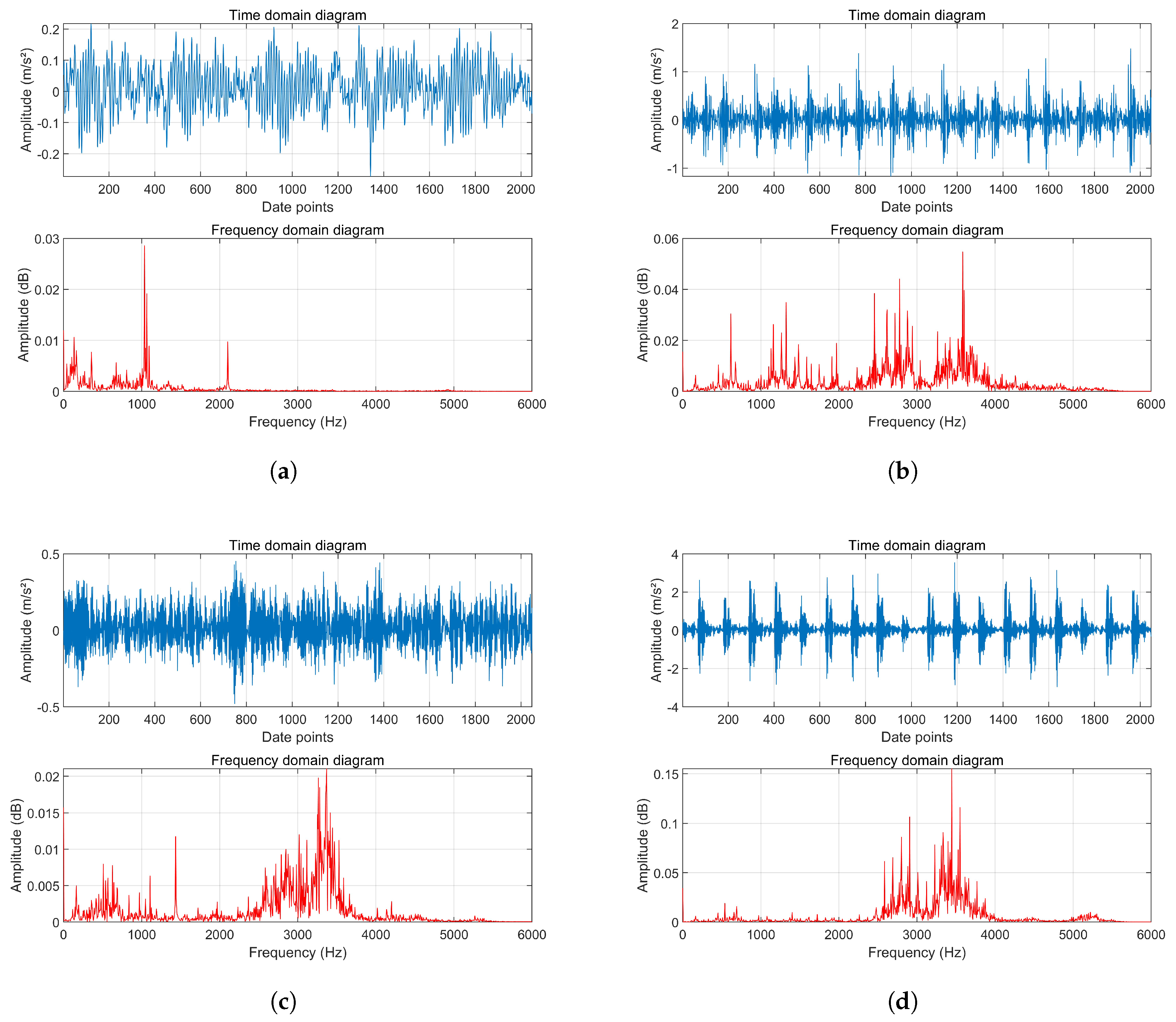
4.2. Signal Processing and Feature Extraction

The minimum permutation/information entropy of each component after VMD decomposition of the vibration signal is used as the fitness function, and OCSSA is employed to determine the parameters α and K in VMD. The ideal parameters selected by the algorithm are displayed in Table 2. The parameters acquired for different vibration signals are considerably scattered, with the decomposition layer number K and the quadratic penalty factor a showing corresponding variations. OCSSA requires 2.3 s per optimization run (Intel i7 CP) due to its population-based search and Cauchy mutation, making it suitable for offline parameter calibration. VMD decomposes a 2048-point signal in 0.02 s (GPU), achieving real-time capability with optimized K = 5–10. BiTCN-Attention achieves 4.8 ms inference latency (NVIDIA 2060 6G GPU) supporting >200 Hz diagnosis, far exceeding the 12 kHz CWRU sampling rate.
In VMD decomposition, since the optimization of the parameter K has a major impact on the decomposition outcome, to further increase the efficacy of the modal components and the accuracy of feature extraction, based on the minimal envelope entropy criterion, the modal function with the lowest envelope entropy number was chosen from the optimized modal components as the research object. Table 2 shows the optimal modal components based on the minimum envelope entropy criterion. Subsequently, nine typical time-domain features are calculated for this modal function, and the results are consolidated into a feature matrix, providing high-quality input features for subsequent fault diagnosis and model construction. This fully demonstrates the superiority of the optimized decomposition and the scientific nature of the feature extraction.

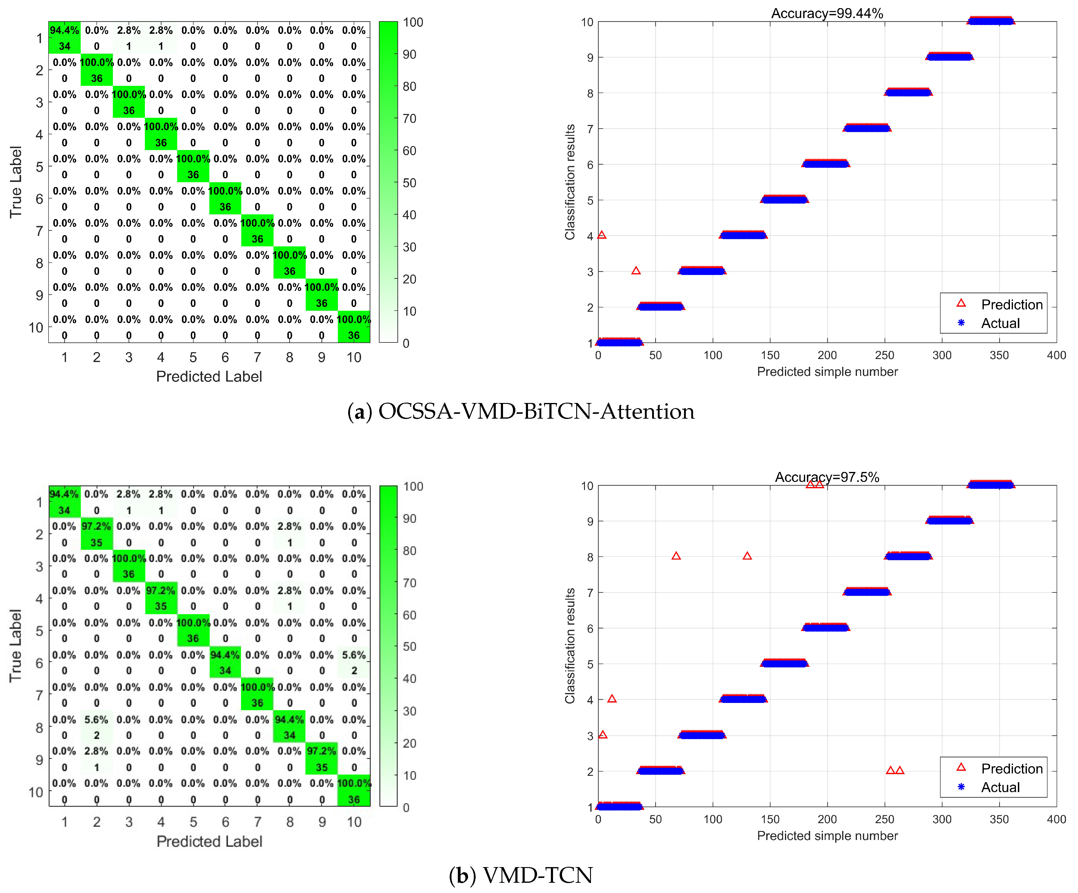
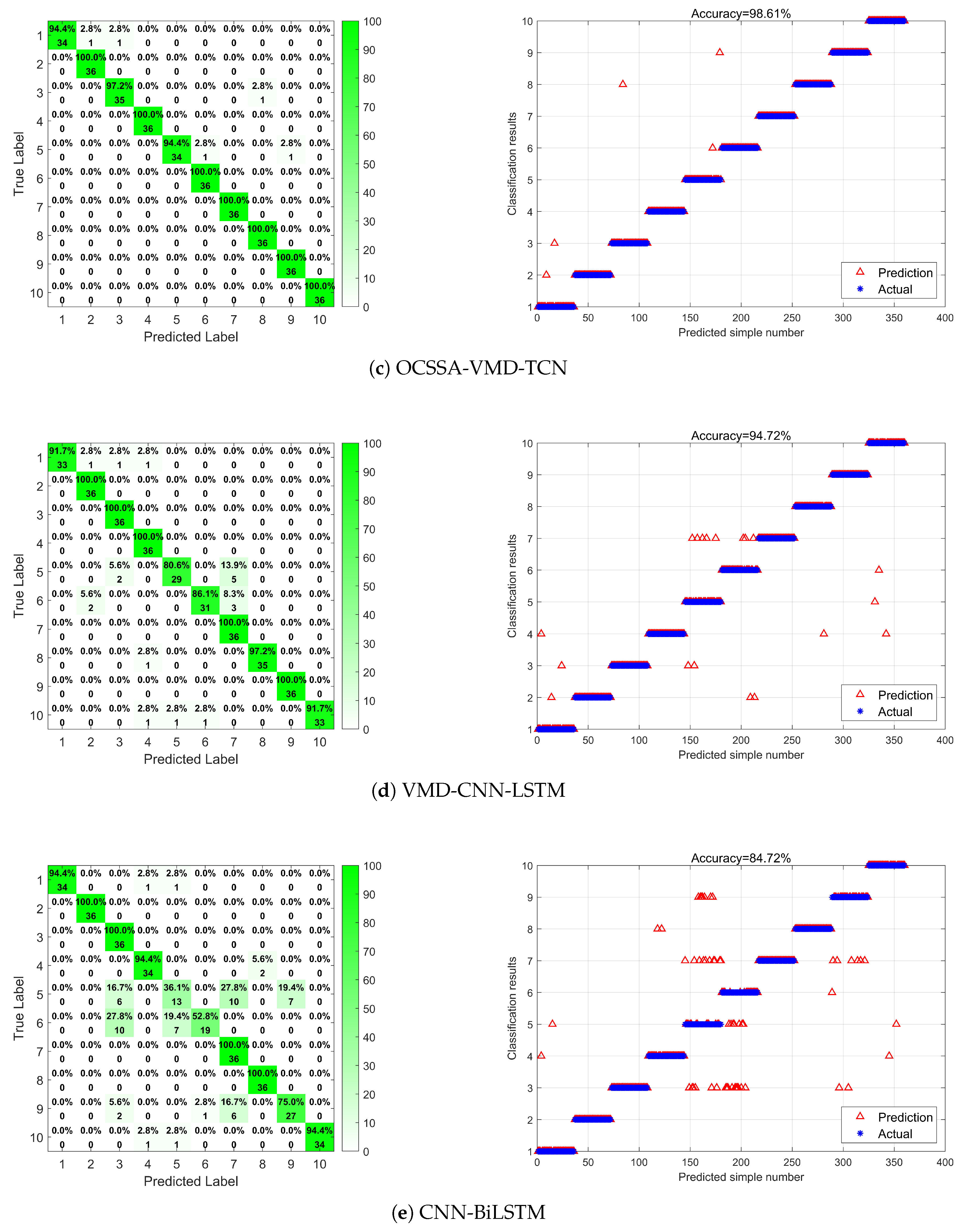
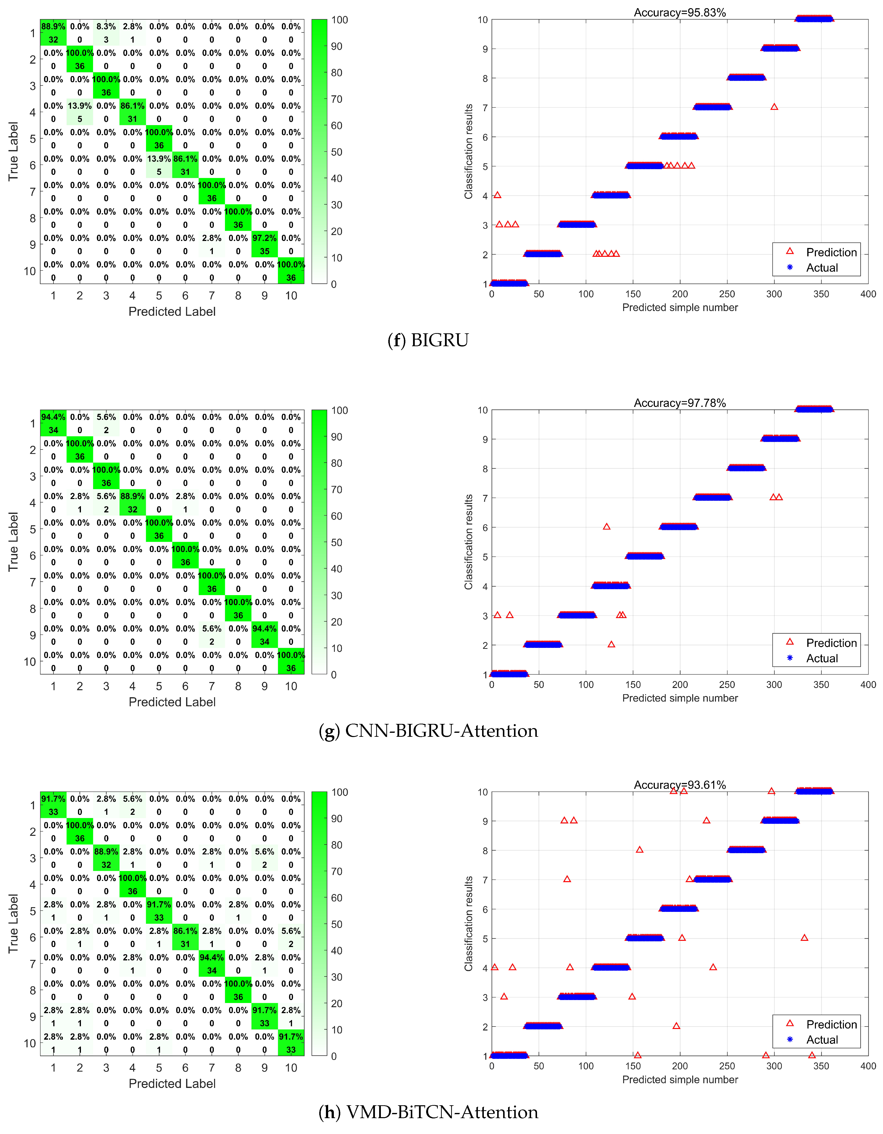
4.3. Comparison with Other Methods

To assess the performance of the OCSSA-VMD-BiTCN-Attention model, a comparison was made with other state-of-the-art fault diagnosis methods, including OCSSA-VMD-TCN, VMD-TCN, VMD-CNN-LSTM, CNN-BiLSTM, BIGRU, and CNN-BIGRU-Attention. The diagnostic conclusions are provided in Figure 9 and Table 3.
As shown in Figure 9 and Table 3, the CNN-BiLSTM and VMD-CNN-LSTM models exhibit limitations in handling complex bearing fault patterns due to insufficient long-term dependency capture and feature fusion, resulting in lower sensitivity (84.72% and 94.72% accuracy) and slower convergence compared to TCN. While the proposed VMD-TCN model improves diagnostic accuracy to 97.5%, its parameter-sensitive VMD decomposition generates disordered IMF components with modal aliasing and pseudo-features, introducing interference in time–frequency analysis. To address these challenges, the OCSSA-BiTCN-Attention framework integrates three innovations: (1) OCSSA optimizes VMD parameters to suppress pseudo-components; (2) BiTCN captures comprehensive temporal dependencies; (3) Attention mechanisms dynamically filter critical fault features. This synergistic approach achieves 99.44% accuracy by eliminating interference while preserving local–global signal characteristics, demonstrating superior robustness, faster detection, and computational efficiency improvement over conventional models, providing a reliable solution for high-precision fault diagnosis under complex industrial conditions.

5. Conclusions

This study proposes a rolling bearing fault diagnosis framework based on OCSSA-optimized VMD and BiTCN-Attention. By integrating OCSSA, VMD parameter adaptive optimization has been achieved, effectively suppressing mode aliasing. BiTCN uses dilated causal convolution to capture the bidirectional temporal features of vibration signals, combined with an attention mechanism to dynamically focus on key fault components, significantly improving the sensitivity of weak faults. The experiment on the CWRU dataset shows that the average diagnostic accuracy of this method for 10 types of faults is 99.44%, which meets the real-time monitoring requirements of industry. This research provides theoretical support and engineering solutions for high-precision fault diagnosis under complex working conditions. In the future, it will further expand to edge computing scenarios through multimodal signal fusion and model lightweight.

Author Contributions

Writing, Y.Y.; methodology, C.H.; validation, G.R.; supervision, T.M.; project administration, J.P. All authors have read and agreed to the published version of the manuscript.

Funding

This work was supported in part by the National Natural Science Foundation of China under Grant 62163002, in part by the Heilongjiang Province Natural Science Foundation under Grant LH2023F051, in part by the Fundamental Research Funds in Heilongjiang Provincial Universities of Qiqihar University under Grant 145409438, and in part by Heilongjiang Province Higher Education Teaching Reform Research Project under Grant SJGY20210946.

Data Availability Statement

The data that support the findings of this study are available from the corresponding author upon reasonable request.

Conflicts of Interest

The authors declare no conflicts of interest.

References

  1. Ran, G.; Chen, H.; Li, C.; Ma, G.; Jiang, B. A Hybrid Design of Fault Detection for Nonlinear Systems Based on Dynamic Optimization. IEEE Trans. Neural Netw. Learn. Syst. 2023, 34, 5244–5254. [Google Scholar] [CrossRef] [PubMed]
  2. Gundewar, S.K.; Kane, P.V. Condition monitoring and fault diagnosis of induction motor. J. Vib. Eng. Technol. 2021, 9, 643–674. [Google Scholar] [CrossRef]
  3. Liu, R.; Yang, B.; Zio, E.; Chen, X. Artificial intelligence for fault diagnosis of rotating machinery: A review. Mech. Syst. Signal Process. 2018, 108, 33–47. [Google Scholar] [CrossRef]
  4. Chen, H.; Luo, H.; Verma, N.; Jiang, B. Guest Editorial: Special Issue on Artificial Intelligence Methods for Maintenance and Safety of Automation Systems. IEEE Trans. Artif. Intell. 2023, 4, 589–591. [Google Scholar] [CrossRef]
  5. Cerrada, M.; Sanchez, R.-V.; Li, C.; Pacheco, F.; Cabrera, D.; de Oliveira, J.V.; Vasquez, R.E. A review on data-driven fault severity assessment in rolling bearings. Mech. Syst. Signal Process. 2018, 99, 169–196. [Google Scholar] [CrossRef]
  6. Pandiyan, M.; Babu, T.N. Systematic Review on Fault Diagnosis on Rolling-Element Bearing. J. Vib. Eng. Technol. 2024, 12, 8249–8283. [Google Scholar] [CrossRef]
  7. Ran, G.; Liu, J.; Li, C.; Lam, H.-K.; Li, D.; Chen, H. Fuzzy-Model-Based Asynchronous Fault Detection for Markov Jump Systems With Partially Unknown Transition Probabilities: An Adaptive Event-Triggered Approach. IEEE Trans. Fuzzy Syst. 2022, 30, 4679–4689. [Google Scholar] [CrossRef]
  8. Atoui, I.; Meradi, H.; Boulkroune, R.; Saidi, R.; Grid, A. Fault detection and diagnosis in rotating machinery by vibration monitoring using FFT and Wavelet techniques. Syst. Signal Process. Their Appl. 2013, 5, 401–406. [Google Scholar]
  9. Rai, A.; Upadhyay, S.H. A review on signal processing techniques utilized in the fault diagnosis of rolling element bearings. Tribol. Int. 2016, 96, 289–306. [Google Scholar] [CrossRef]
  10. Li, D.Y.; Dong, J.; Peng, K.X. Motor fault classification using hybrid short-time Fourier transform and wavelet transform with vibration signal and convolutional neural networkA Novel Adaptive STFT-SFA Based Fault Detection Method for Nonstationary Processes. IEEE Sens. J. 2023, 23, 10748–10757. [Google Scholar] [CrossRef]
  11. Wu, F.; Qu, L. Diagnosis of subharmonic faults of large rotating machinery based on EMD. Mech. Syst. Signal Process. 2009, 23, 467–475. [Google Scholar] [CrossRef]
  12. Shifat, T.A.; Hur, J.W. EEMD assisted supervised learning for the fault diagnosis of BLDC motor using vibration signal. J. Mech. Sci. Technol. 2020, 34, 3981–3990. [Google Scholar] [CrossRef]
  13. Dragomiretskiy, K.; Zosso, D. Variational Mode Decomposition. IEEE Trans. Signal Process. 2014, 62, 531–544. [Google Scholar] [CrossRef]
  14. Chen, H.; Zhong, K.; Ran, G.; Cheng, C. Deep Learning-Based Machinery Fault Diagnostics. Machines 2022, 10, 690. [Google Scholar] [CrossRef]
  15. Shen, Q.; Zhang, Z. Fault Diagnosis Method for Bearing Based on Attention Mechanism and Multi-Scale Convolutional Neural Network. IEEE Access 2024, 12, 12940–12952. [Google Scholar] [CrossRef]
  16. Wen, L.; Li, X.Y.; Gao, L.; Zhang, Y.Y. A New Convolutional Neural Network-Based Data-Driven Fault Diagnosis Method. IEEE Trans. Ind. Electron. 2018, 65, 5990–5998. [Google Scholar] [CrossRef]
  17. Ding, F.; Li, X.; Qu, J.X. ault diagnosis of rolling bearing based on improved CEEMDAN and distance evaluation technique. J. Vibroeng. 2017, 19, 260–275. [Google Scholar] [CrossRef]
  18. Chen, X.; Zhang, B.; Gao, D. Bearing fault diagnosis base on multi-scale CNN and LSTM model. J. Intell. Manuf. 2021, 32, 971–987. [Google Scholar] [CrossRef]
  19. Pan, H.H.; He, X.X.; Tang, S.; Meng, F.M. An Improved Bearing Fault Diagnosis Method using One-Dimensional CNN and LSTM. Stroj. Vestn. J. Mech. Eng. 2018, 64, 443–452. [Google Scholar]
  20. Khorram, A.; Khalooei, M.; Rezghi, M. End-to-end CNN+LSTM deep learning approach for bearing fault diagnosis. Appl. Intell. 2021, 51, 736–751. [Google Scholar] [CrossRef]
  21. Jiao, J.; Zhao, M.; Lin, J.; Liang, K. A comprehensive review on convolutional neural network in machine fault diagnosis. Neurocomputing 2020, 417, 36–63. [Google Scholar] [CrossRef]
  22. Song, Y.; Gao, S.; Li, Y.; Jia, L.; Li, Q.; Pang, F. Distributed Attention-Based Temporal Convolutional Network for Remaining Useful Life Prediction. IEEE Internet Things J. 2021, 8, 9594–9602. [Google Scholar] [CrossRef]
  23. Shang, Z.W.; Liu, H.; Zhang, B.R.; Feng, Z.H.; Li, W.X. Multi-view feature fusion fault diagnosis method based on an improved temporal convolutional network. Insight 2023, 65, 559–569. [Google Scholar] [CrossRef]
  24. Xing, J.Q.; Xu, J.X. An Improved Convolutional Neural Network for Recognition of Incipient Faults. IEEE Sens. J. 2022, 22, 16314–16322. [Google Scholar] [CrossRef]
  25. Huang, Y.; Wang, A.; Jiao, J.; Xie, J.; Chen, H. Short-Term PV Power Forecasting Based on CEEMDAN and Ensemble DeepTCN. IEEE Trans. Instrum. Meas. 2023, 72, 2526012. [Google Scholar] [CrossRef]
  26. Xue, J.; Shen, B. A novel swarm intelligence optimization approach: Sparrow search algorithm. Syst. Sci. Control Eng. 2020, 8, 22–34. [Google Scholar] [CrossRef]
  27. Wen, X.D.; Liu, X.D.; Yu, C.H.; Gao, H.N.; Wang, J.; Liang, Y.J.; Yu, J.L.; Bai, Y. IOOA: A multi-strategy fusion improved Osprey Optimization Algorithm forglobal optimization. Electron. Res. Arch. 2024, 32, 2033–2074. [Google Scholar] [CrossRef]
  28. Li, C.; Liu, Y.; Zhou, A.; Kang, L.; Wang, H. A Fast Particle Swarm Optimization Algorithm with Cauchy Mutation and Natural Selection Strategy. Adv. Comput. Intell. 2007, 1, 334–343. [Google Scholar]
  29. Case Western Reserve University Bearing Data Center. Bearing Data Set. Available online: https://engineering.case.edu/bearingdatacenter (accessed on 21 November 2024).
Figure 1. TCN network.
Actuators 14 00218 g001
Figure 2. Causal convolution.
Actuators 14 00218 g002
Figure 3. Extended convolution.
Actuators 14 00218 g003
Figure 4. Residual module architecture of TCN.
Actuators 14 00218 g004
Figure 5. BiTCN network.
Actuators 14 00218 g005
Figure 6. BiTCN residual block.
Actuators 14 00218 g006
Figure 7. CWRU motor bearing test bench.
Actuators 14 00218 g007
Figure 8. Time-frequency domain diagrams of vibration signals for different types of rolling bearings: (a) load normal, (b) inner race fault at 0.1778 mm, (c) rolling element fault at 0.1778 mm, (d) outer race fault at 0.1778 mm.
Actuators 14 00218 g008
Figure 9. Prediction accuracy plots for bearing fault prediction using different models: (a) OCSSA-VMD-BiTCN-Attention, (b) VMD-TCN, (c) OCSSA-VMD-TCN, (d) VMDCNN-LSTM, (e) CNN-BiLSTM, (f) BIGRU, (g) CNN-BIGRU-Attention, (h) VMD-BiTCN-Attention.
Actuators 14 00218 g009aActuators 14 00218 g009bActuators 14 00218 g009c
Table 1. Fault dataset.
Fault TypeFault Diameter (mm)Training SampleTest SampleSample Data SizeFault Label
Normal-84036020481
Inner ring fault0.177884036020482
Rolling ball fault0.355684036020483
Outer ring fault0.533484036020484
Inner ring fault0.177884036020485
Rolling ball fault0.355684036020486
Outer ring fault0.533484036020487
Inner ring fault0.177884036020488
Rolling ball fault0.355684036020489
Outer ring fault0.5334840360204810
Table 2. Optimal parameters.
Fault TypeFault Diameter (mm)Optimum Solutions α Optimum Solutions KOptimum Parameters
Normal-9051010
Inner ring fault0.17782000101
Rolling ball fault0.355635471
Outer ring fault0.533410091
Inner ring fault0.1778100101
Rolling ball fault0.35562144104
Outer ring fault0.53342500101
Inner ring fault0.17782491101
Rolling ball fault0.3556176851
Outer ring fault0.53342039101
Table 3. Accuracy of different methods.
MethodsType1Type2Type3Type4Type5Type6Type7Type8Type9Type10Average
OCSSA-VMD-BiTCN-Attention94.4%100%100%100%100%100%100%100%100%100%99.44%
OCSSA-VMD-TCN94.4%97.2%100%97.2%100%94.4%100%94.4%97.2%100%97.5%
VMD-TCN94.4%100%97.2%100%94.4%100%100%100%100%100%98.61%
VMD-CNN-LSTM91.7%100%100%100%80.6%86.1%100%97.2%100%91.7%94.72%
CNN-BiLSTM94.4%100%100%94.4%36.1%52.8%100%100%75%94.4%84.72%
BIGRU88.9%100%100%86.1%100%86.1%100%100%97.2%100%95.83%
CNN-BIGRU-Attention94.4%100%100%88.9%100%100%100%100%94.4%100%97.78%
VMD-BiTCN-Attention91.7%100%88.9%100%91.7%86.1%94.4%100%91.7%91.7%93.61%
Disclaimer/Publisher’s Note: The statements, opinions and data contained in all publications are solely those of the individual author(s) and contributor(s) and not of MDPI and/or the editor(s). MDPI and/or the editor(s) disclaim responsibility for any injury to people or property resulting from any ideas, methods, instructions or products referred to in the content.

