Three-Dimensional Modified Cross-Section Hydrofoil Design and Performance Study

Abstract

To improve the hydrodynamic performance of hydrofoils, this study combines the shape characteristics of flat and elliptical wings, uses parabolic function to fit the leading and trailing edges of hydrofoils, introduces the cross-section coefficient λ to characterize the cross-sectional size of hydrofoils along the spreading direction, and designs five hydrofoils with different cross-sections. The motion of the hydrofoil is simulated using the finite element analysis software Fluent to obtain the hydrodynamic performance curve of the hydrofoil and analyze the effect of different end face sizes on the performance of the hydrofoil. The results show that compared with the flat wing, the peak drag of the variable section hydrofoil with λ = 0.5 is reduced by 9.3%, the pitching moment is reduced by 23.1%, and the average power is raised by 17.4%. If the appropriate reduction in the cross-section coefficient is too small, it will exacerbate the wing tip vortex shedding, the hydrofoil surface pressure will be too concentrated, and the hydrofoil motion stability will be reduced. The lift coefficient, drag coefficient, and pitching moment coefficient of the hydrofoil are positively correlated with the cross-section coefficient λ, and positively correlated with the motion frequency.

1. Introduction

Against the backdrop of growing global energy demand, the increased global consumption of fossil fuels and increased carbon emissions are causing global warming and environmental damage. The development of new energy sources has become one of the most important initiatives to promote sustainable economic development. The ocean accounts for about 71% of the total area of the earth, nurturing a huge ecosystem, rich in mineral and energy resources; of which only 5% of the area has been explored, therefore, the ocean has a huge potential for development, and can provide a strong guarantee for human energy supply. Ocean energy mainly includes tidal energy, tidal energy, wave energy, seawater temperature difference energy, seawater salt difference energy [1,2].

Initially many scientists designed and built prototypes to simulate the feasibility of using hydrofoils to generate electricity. McKinney first proposed the theory about using airfoils to capture the energy of fluids in 1981 [3]. Kinsey gave the parameters about measuring the performance of hydrofoil energy capture. Subsequently, many scholars worked on the hydrofoil energy capture performance [4]. In 2003, a 150 kW oscillating hydrofoil tidal energy generator was tested in Scottish waters. Dag Herman et al. tested a turbine applying a new flexible wing, achieving a peak power coefficient of 0.37, and proved that the device had a self-starting capability at low flow velocities of $v=0.5$ m/s [5]. Zhen Liu and Hengliang Qu studied the performance of tandem hydrofoil devices made of aluminum alloy to capture energy from water flow. The peak power coefficients of the upstream and downstream hydrofoils increased by 65.7% and 48.0% compared to a single hydrofoil, and their efficiencies increased by 48.0% and 15.4%, respectively [6]. Laetitia Pernod and Antoine Ducoin et al. investigated the fluid–structure coupling and hydroelastic response of composite hydrofoils using an innovative joint experimental and numerical approach. They invented a novel material for making hydrofoils, which is designed as a sandwich composite structure, that is, a structure made of two thin skins attached on both sides of a lightweight core. The advantages of composites over metals for hydrofoil materials are that they are lightweight, strong, corrosion-resistant, and easy to shape, which provides superior hydrodynamic performance and longer service life [7]. Y. S. Zeng and Z. F. Yao et al. investigated the effect of trailing edge shape on the added mass and hydrodynamic damping of hydrofoils. The hydrofoil was tested at a flow rate of 20 m/s and a mean hydrofoil surface ${\mathrm{y}}^{+}$ value of 1.27, and the experimental and numerical results show that the hydrofoils have a strong hydroelasticity response. Hydrofoils vibrate periodically in the water, which is a dynamic response that gradually decays due to damping. Fluid–structure coupling and vortex shedding effects were observed and the result shows that collisions between the upper and lower trailing edge vortices lead to faster dissipation of the vortex strength, which increases the hydrodynamic damping ratio of the Donaldson trailing edge [8].

With the development of computational fluid dynamics, scientists are studying hydrofoils in a richer and more diverse way. According to the motion form of the hydrofoil, hydrofoil motion can be classified as active, semi-active, passive [7,8]. Xia Wu et al. used particle image velocimetry and computational fluid dynamics to study the effects of Reynolds number, motion frequency, and oscillation amplitude on the energy capture performance of hydrofoils. They concluded that the mean thrust coefficient increases with the increase in the dimensionless frequency, and that this law is independent of factors such as the blade motion pattern, the motion profile and flexibility [9]. Yubing Zhang et al. investigated the energy capture performance of a two-dimensional flexible hydrofoil in semi-active mode, and found that the average power coefficient of the flexible hydrofoil can be increased by as much as 36% at 20% flexible amplitude compared to a rigid hydrofoil [10]. Tuyen Quang Le et al. found that 3D flexible hydrofoils also improved the power extraction efficiency, but the enhancement was smaller than that of 2D hydrofoils, about 15%, because of the attenuating effects of 3D effects (e.g., end losses and spreading vortices) [11]. Zhen Liu et al. established and validated a two-dimensional numerical model of hydrofoils in shear flow by studying the hydrodynamic performance of semi-active hydrofoils. Two control methods are proposed: damping block control method and linear spring control method [12]. A non-sinusoidal waveform trajectory profile was proposed by Qin Xiao and Liao Wei for improving the energy extraction performance of hydrofoils. They combined the designed trapezoidal pitching motion with the sinusoidal waveform pitching motion to design a new trajectory, which maximized the energy extraction efficiency of the non-sinusoidal hydrofoil by 50% compared with the sinusoidal hydrofoil [13]. Derrick Custodio and Charles Henoch et al. investigated the cavitation characteristics and hydrodynamics of hydrofoils with wavy leading edges and showed that cavitation in the modified hydrofoils with larger amplitude was confined to the region directly behind the protruding slots, whereas the baseline model and the hydrofoils with smaller amplitudes exhibited piecewise cavitation throughout the entire span [14]. Jianxin Hu and Qing Xiao investigated the influence of three-dimensional effects on the hydrodynamic performance of hydrofoils, and found that the use of endplates can reduce the three-dimensional effects, and when the chord spread ratio is greater than 10, the energy capture efficiency of the hydrofoils can be reduced to less than 10% [15].

At this stage, wings can be classified into flat, elliptical, trapezoidal, delta, swept-back, variable swept-back, and forward-swept wings according to the shape of the plane when viewed from the top [16]. As shown in Figure 1, the flat wing construction is simple and easy to process; the wing produces higher lift power, but the drag torque is larger in order to ensure that the case of lift as low as possible drag. The flat wing can have a little bit of taper, from the inside to the outside of the gradual narrowing, which gives rise to trapezoidal wings, swept-back wings and other types of wing, but essentially is still a flat wing, and the disadvantages of higher drag and torque are still more apparent [17,18]. Elliptical wings generally have less drag and lift than flat wings but are not able to satisfy higher requirements of lift [18]. Compared with a straight wing, a hydrofoil with a leading edge bump has a higher lift-to-drag ratio and a larger stall angle, especially at large angles of attack, which reduces drag and saves energy more significantly [19]. ZHANG Zhi-jun and LI Tian-ge studied the laminar separation phenomenon and flow field structure of elliptical airfoils at low Reynolds numbers. The results show that at low Reynolds numbers, the laminar separation bubbles at the leading edge of thin elliptical airfoils at small angles of attack are the reason for their high lift coefficient and lift-to-drag ratio. As the Reynolds number increases, the separation bubbles appear at the leading edge of the thin elliptical airfoils, but the shape is reduced, while at lower Reynolds numbers, the thin elliptical airfoils do not have turning reattachment at small angles of attack; meanwhile, the appearance of laminar separation bubbles also has an important effect on the size and location of the separation vortices at the trailing edge of the airfoils. The relative thickness and Reynolds number change the aerodynamic characteristics of elliptical airfoils by affecting the size and position of laminar vesicles on the upper surface and the morphology of the trailing edge vortices [20,21]. At small angles of approach, the lift of the forward swept wing is small because the vortex of the wing tip of the sweptback wing is able to interfere favorably with the adherent flow on the surface of the wing, i.e., vortex lift: at medium angles of approach, the vortex breaks up as the wingtip separation of the backward swept wing intensifies, so that lift begins to fall, while at this time, the lift of the forward swept wing still maintains a slow growth; at large angles of approach, the forward swept wing has a large lift and a slow fall with good aerodynamic performance at large angles of approach [22]. Various types of airfoils are improved based on flat airfoils, and hydrofoils with different appearances can meet the demands of specific working conditions.

The study of hydrodynamics and energy capture performance of oscillating hydrofoils is the theoretical basis to guide the design of the oscillating hydrofoil energy capture system. Most of the existing hydrofoil research focuses on two-dimensional hydrofoils, flexible hydrofoils, and fixed-section hydrofoils, with less research on variable section hydrofoils [23]. The study of variable cross-section hydrofoils can provide guidance for future research on the three-dimensional effects of hydrofoils, and also references the selection of hydrofoil chord spread ratio.

Compared with flat hydrofoils, variable section hydrofoils have the following advantages and are more suitable for tidal energy generating devices. First, the mass of the variable section hydrofoil is lower, which can reduce the motion inertia of the device [24]. Second, the pitching moment of the variable section hydrofoil is lower, and the pressure distribution is more uniform, which effectively reduces the moment attached to the hydrofoil’s rotating axis by the water flow and makes the hydrofoil’s movement smoother [25]. Third, compared with ordinary fixed-section hydrofoils, variable section hydrofoils have higher energy capture efficiency, which can improve the efficiency of the device.

Unlike other studies, the hydrofoil designed in this paper focuses on the cross-sectional variation in the hydrofoil, and introduces a cross-sectional coefficient $\lambda$ to characterize the geometry of the hydrofoil. The designed geometry is able to reduce the projected area and mass of the hydrofoil while increasing the energy trapping efficiency of the hydrofoil, and decreasing the drag coefficient, and the pitch moment coefficient, which is a guideline for the design of future hydrofoil power generation devices.

This paper is organized as follows. Section 2 describes the kinematic model of the oscillating hydrofoil and the variable cross-section hydrofoil design scheme. Section 3 shows the validation process of the simulation model. Section 4 shows the simulation results of the variable section hydrofoil with different parameters. Section 5 shows the conclusions of the study.

2. Geometry and Models of Motion

2.1. Hydrofoil Motion Model

The non-stationary flow field around the oscillating hydrofoil is turbulent, the fluid in the turbulent field can be regarded as a continuous medium, and the instantaneous control equation of the flow field around the oscillating hydrofoil is the Navier–Stokes equation. The fluid around the oscillating hydrofoil is regarded as an incompressible fluid [4]. In this paper, the hydrofoil is assumed to be in the midst of a stable fluid with a characteristic velocity $U_{\infty }$. It is assumed that the density of the fluid remains constant under all conditions and the fluid is incompressible. The flow process has only liquid terms and the flow process does not involve heat transfer. The mass equation and momentum conservation equation in tensor form in the inertial coordinate system can be obtained as follows:

$$\partial u_i/\partial x_i=0,$$

(1)

$$\begin{array}{c}\partial u_i/\partial t+u_j·\partial u_i/\partial x_j=F_i-\partial p/\left(\partial x_i·\rho \right)+\nu {\nabla }^2{u}_i,\end{array}$$

(2)

where $\rho$ is the fluid density, $t$ is the time, $p$ is the static pressure, $x_i$ (for a three-dimensional flow field, i = 1, 2, 3) is the coordinate axis, $F_i$ is the component of the volume force in the i-direction, and $u_i$ is the component of the fluid velocity along the i-direction.

The static pressure $C_{po}$ is a dimensionless number that describes the relative pressure spread throughout the flow field in fluid dynamics, the static pressure $C_{po}$ can be calculated by the following equation:

$$\begin{array}{c}{C}_{po}=\left(P-P_{\infty }\right)/0.5\rho {U_{\infty }}^2=\left(P-P_{\infty }\right)/\left(P_0-P_{\infty }\right),\end{array}$$

(3)

where $P$ is the pressure on the surface of the object, $P_{\mathrm{\infty }}$ is the free-flow windward static pressure, and $U_{\mathrm{\infty }}$ is the inlet velocity. The hydrofoil motion model and force analysis are shown in Figure 2 [26,27]. The hydrofoil chord length is $c$. In this paper, it is assumed that the hydrofoil only performs heave and pitch motions. Under the action of the water current with horizontal velocity $U_{\infty }$, the hydrofoil bears the water current impact at a certain angle of attack, and is subjected to the combined force $F\left(t\right)$. This is decomposed into the lift force $L\left(t\right)$, the moment$M\left(t\right)$, and the drag force $D\left(t\right)$, with the center of the force distance and the point of force action at the point $O$, in which the drag force $D\left(t\right)$ is in the same direction of the incoming flow, and the lift force$L\left(t\right)$ is perpendicular to the direction of the incoming flow. The hydrofoil is constrained at point $O$ to having degrees of freedom in the spreading direction, so that it can move in the direction of lift and rotate around point $O$. The hydrofoil can move in the direction of lift and rotate around point $O$ under ideal conditions. Under ideal conditions, the lift $L\left(t\right)$ and torque $M\left(t\right)$ work and the drag$D\left(t\right)$ does not.

The motion of the hydrofoil in the water is synthesized by the pitching motion $\theta \left(t\right)$ around the pitch axis of the hydrofoil and the lifting and sinking motion $y\left(t\right)$ in the vertical direction, with the maximum displacement of the hydrofoil as $y_0$, the maximum angle of rotation as ${\theta }_0$, the movement frequency as $f$, and the phase difference between the pitching and lifting and sinking motions as $\phi$ [28].

$$\begin{array}{c}y\left(t\right)=y_{0}sin\left(2\pi ft+\phi \right),\end{array}$$

(4)

$$\begin{array}{c}\theta \left(t\right)={\theta }_0\sin \left(2\pi ft\right).\end{array}$$

(5)

In order to avoid the problems caused by different hydrofoil chord lengths and flow velocity variations, dimensionless reduced frequencies $f^{\mathrm{*}}$ are introduced and defined as [4,29]:

$$\begin{array}{c}{f}^{*}=fc/U_{\infty }.\end{array}$$

(6)

In the software Fluent 2020R1, the physical model is discretized into a finite number of grid units, and the finite element interpolation method is used to find the surface velocity distribution of the hydrofoil. Then, the instantaneous lift $L\left(t\right)$, instantaneous drag $D\left(t\right)$, and instantaneous moment $M\left(t\right)$ of the hydrofoil are obtained according to Bernoulli’s equation, and the dimensionless coefficient of the hydrofoil. The instantaneous lift coefficient $C_L\left(t\right)$, instantaneous drag coefficient $C_D\left(t\right)$, and instantaneous moment coefficient $C_M\left(t\right)$ are [27]:

$$C_L\left(t\right)=L\left(t\right)/{\displaystyle \frac{1}{2}}\rho U_{\infty }^{2}S,$$

(7)

$$C_D\left(t\right)=D\left(t\right)/{\displaystyle \frac{1}{2}}\rho U_{\infty }^{2}S,$$

(8)

$$C_M\left(t\right)=M\left(t\right)/{\displaystyle \frac{1}{2}}\rho U_{\infty }^{2}Sc,$$

(9)

where $\rho$ is the water density, $S$ is the projected area of the hydrofoil, $s=cd$ when the hydrofoil cross-section is constant, and $d$ is the hydrofoil spread length.

Define the power of the lifting and sinking motion of the hydrofoil as $P_L\left(t\right)$, and the power of the pitching motion as $P_M\left(t\right)$. Since the hydrofoil has no displacement in the direction of drag, the total power of the hydrofoil motion, $P\left(t\right)$, is the sum of the power of the lifting and sinking motion and the power of the pitching motion, and the equation is defined as follows [30]:

$$P_L\left(t\right)=L\left(t\right)\ast \dot{y\left(t\right),}$$

(10)

$$P_M\left(t\right)=M\left(t\right)\ast \dot{\theta \left(t\right),}$$

(11)

$$P\left(t\right)=P_L\left(t\right)+P_M\left(t\right).$$

(12)

The instantaneous power coefficients$C_P$, the average power coefficients ${\overline{C}}_P$, the average drag coefficient ${\overline{C}}_D$, and average lift coefficient ${\overline{C}}_L$ for hydrofoils are defined as follows [11]:

$$C_P=2\left[P_L\left(t\right)+P_M\left(t\right)\right]/\rho U_{\infty }^{3}S,$$

(13)

$${\overline{C}}_P={\overline{C}}_{PL}+{\overline{C}}_M=(1/T){\int }_0^T\left[C_L\left(t\right)\nu \left(t\right)/U_{\infty }\right]dt+(1/T){\int }_0^T\left[{cC}_M\left(t\right)\phi \left(t\right)/U_{\infty }\right]dt,$$

(14)

$${\overline{C}}_D=\left[{\int }_0^T{C}_D\left(t\right)dt\right]/T,$$

(15)

$${\overline{C}}_L=\left[{\int }_0^T{C}_L\left(t\right)dt\right]/T.$$

(16)

2.2. Hydrofoil Design

NACA 0015 is a very mature airfoil widely used in aerospace and marine applications and using this airfoil as a base can avoid some unnecessary mistakes [31]. Based on the existing NACA 0015 airfoil, this paper combines the characteristics of flat and elliptical airfoils, and controls the leading and trailing edges of the hydrofoils with parabolic function, which retains the shape characteristics of flat and elliptical airfoils, respectively. The profile of the variable section hydrofoil is shown in Figure 3. The variable section hydrofoil is a symmetric hydrofoil with the cross-sectional area gradually reduced from the middle to the ends, the chord length of the middle section hydrofoil chord is $c=0.24 \mathrm{m}$, the chord lengths of the left and right hydrofoil chords are $c_0=\lambda c$, and the position of the pitch axis of the hydrofoil is at the distance from the leading edge of the hydrofoil at the place of $1/3$. Respectively to the pitch axis of the hydrofoil, the horizontal projection line of the middle section for the x, y axis to establish a right-angle coordinate system, with a parabolic function to control the size of the hydrofoil cross-section, to obtain the curve equations such as Equations (17) and (18). In this study, the 3D engineering drawing software UG 12.0 is used to design the variable section hydrofoil, and the 3D hydrofoil is shown in Figure 3.

$$y_1\left(x\right)=4x^2(\lambda -1)/75c+{\displaystyle \frac{c}{3}},$$

(17)

$$y_2\left(x\right)={8x}^2(1-\lambda )/75c-{\displaystyle \frac{2c}{3}}.$$

(18)

The hydrofoil projection area $S$ is defined as follows:

$$S={\int }_{-2.5c}^{2.5c}\left[y_1\left(x\right)-y_2\left(x\right)\right]dx=5(\lambda +2)c^2/3.$$

(19)

By varying the value of λ, the hydrofoil areas at different end-states are obtained as shown in

Table 1. Projected area of hydrofoils with different end-states.

λ Value	Hydrofoil Projected Area S (m2)
1	0.288
0.9	0.2984
0.8	0.2688
0.7	0.2592
0.6	0.2496
0.5	0.2400

:

In the reference [4], A symmetrical watershed model of $75 c\times 70 c\times 30 c$ is selected, and the same size of the watershed is selected for simulation in this paper. As shown in Figure 4, using the overlapping grid technology, the model grid is divided into the background grid and the component grid. Each grid area overlaps spatially, but there is no connectivity. They are independent of each other and must be completed by the pre-processing software digging holes, matching interpolation points, and other operations, to establish a connectivity relationship. The preprocessor will overlap the grid into a cell unit, discrete (computational) units, and interpolation units. The fluid control equations in the background grid and parts of the respective grid for solving. The interpolation unit constitutes the internal boundary condition, which is used to transfer data, and ultimately obtain the entire computational information of domain of the flow field. The overlapping grid technique requires double precision processing, which has high requirements on the grid quality, and the grid division of the overlapping region must be meticulously planned to provide uniform, high-quality grids, or else it is prone to produce isolated cells, resulting in inaccurate data transfer [4]. The meshing details are shown in Figure 4. The Spalart–Allmaras model (S-A model for short) is mainly used to solve the wall-bound flow, which has good applications in the simulation of external flow field in aerospace and turbomachinery turbulence simulation [10]. The S-A model can be effective in solving the low Reynolds number flow, such as the viscous-influenced region in the boundary layer. In the reference [4], the S-A turbulence model is used in this study to turn on the mesh adaption to make the fluid parameters in the overlapping region smoothly distributed in order to achieve a better interpolation effect. Then, the pressure-based basin solver is used, the pressure-velocity coupling method uses coupled model. The discretization format of pressure, momentum, and turbulent viscous coefficients is chosen as second-order windward format, and the time discretization adopts the first-order implicit format, the continuity and velocity are used as the first-order discretization format. The absolute convergence criteria of continuity and velocity residuals are 10⁻⁴ and 10⁻⁵, respectively. The motion of the hydrofoil is controlled, and the moment data are extracted by writing a UDF file.

3. Algorithm Validation

3.1. Process Verification

In this paper, we refer to the reference [4] for the calculation of data. To verify the correctness of the selected computational model, the parameters of the computational model are: ${ \theta }_0=75°$, $y_0/c=1, f^{*}=0.14,\nu =1\times {10}^{-6}{\mathrm{m}}^2/\mathrm{s}, c=0.25 \mathrm{m}, {Re}_c=\mathrm{500,000}, X_P/c=1/3, \phi =90°, d/c=5$, the convergence error is${ 10}^{-5}$. Referring to Ref. [4], we set the number of the background grids for meshing to 960 thousand, the number of the part. The number of meshes was 4000 thousand, the time step t = T/1000, and five cycles were calculated. The comparison of the computational results with references for the third, fourth, and fifth cycles selected after the computational results reach periodicity is shown in

Table 2. Comparison of Literature Data.

		${\overline{\mathit{C}}}_{\mathit{D}}$	${\widehat{\mathit{C}}}_{\mathit{L}}$	${\widehat{\mathit{C}}}_{\mathit{M}}$	${\overline{\mathit{C}}}_{\mathit{P}}$
Results from the reference [4]		1.546	2.601	0.507	0.811
Results of this paper	Third cycle	1.544	2.609	0.505	0.815
	Fourth cycle	1.554	2.616	0.518	0.819
	Fifth cycle	1.548	2.613	0.513	0.814

. The results show that under the same parameter conditions, the calculation results of this paper are similar to those of the reference [4] with the same parameters, and the procedure is correct.

In order to verify the effects of different turbulence models on the hydrodynamic performance of 3D hydrofoils and to select a more suitable turbulence model, the S-A, k-$\mathsf{\omega }$, and SST models were initially selected for the simulation experiments under the same working conditions mentioned above. The coefficient values of the third, fourth, fifth, and sixth cycles after the hydrofoil motion is stabilized are selected for comparison, and the results are shown in

Table 3. Result of simulation coefficients for different turbulence models.

Turbulence Model	${\overline{\mathit{C}}}_{\mathit{D}}$				${\widehat{\mathit{C}}}_{\mathit{L}}$				${\overline{\mathit{C}}}_{\mathit{P}}$
	$3\mathbf{rd} \mathbf{T}$	$4\mathbf{th} \mathbf{T}$	$5\mathbf{th} \mathbf{T}$	$6\mathbf{th} \mathbf{T}$	$3\mathbf{rd} \mathbf{T}$	$4\mathbf{th} \mathbf{T}$	$5\mathbf{th} \mathbf{T}$	$6\mathbf{th} \mathbf{T}$	$3\mathbf{rd} \mathbf{T}$	$4\mathbf{th} \mathbf{T}$	$5\mathbf{th} \mathbf{T}$	$6\mathbf{th} \mathbf{T}$
S-A	1.52	1.52	1.51	1.53	2.60	2.61	2.61	2.62	0.81	0.80	0.81	0.81
k-$\mathsf{\omega }$	1.56	1.51	1.47	1.42	2.70	2.71	2.60	2.51	0.78	0.81	0.83	0.84
SST	1.61	1.55	1.50	1.51	2.51	2.54	2.63	2.67	0.82	0.81	0.81	0.85

. The experimental results show that the peak lift coefficient, average drag coefficient and average power coefficient of the k-w and SST models fluctuate greatly, while the coefficients of the S-A model are more stable. In addition, in the simulation parameter setting, the k-$\mathsf{\omega }$ model and SST model need to increase the convergence error to ${10}^{-2}$ to make the simulation converge, so the S-A turbulence model is selected for the subsequent experiments in this paper.

3.2. Grid Number and Time Step Validation

Near the hydrofoil boundary, the flow velocity varies greatly, and the grid resolution is required to be high, but too many grids not only improve the accuracy, but also prolong the solution time. To verify that the divided grid size has less influence on the simulation values, six models with different numbers of part grids are divided to verify the grid independence, and the experimental parameters are the same as those in Section 3.1. The following table shows the number of grids, and the ${y }^{+}$ value of the first layer of the hydrofoil wall in each grid model is controlled to remain around 1 as far as possible. The experimental parameters are the same, the time step is T/1000, and six cycle steps are calculated. After the calculation reaches periodicity, the result of the fifth cycle is selected for comparison. The calculation results are shown in

Table 4. Comparison of different grid quantity factors.

Number of Cells	${\overline{\mathit{C}}}_{\mathit{D}}$	${\widehat{\mathit{C}}}_{\mathit{L}}$	${\widehat{\mathit{C}}}_{\mathit{M}}$	${\overline{\mathit{C}}}_{\mathit{P}}$
3,000,000	1.541	2.615	0.511	0.812
3,500,000	1.555	2.616	0.518	0.794
4,000,000	1.561	2.621	0.523	0.811
4,700,000	1.552	2.612	0.519	0.809
8,000,000	1.553	2.619	0.521	0.810
12,000,000	1.550	2.620	0.520	0.811

.

The differences in the calculated coefficients for the six grid number models are 1.3% for the average drag ${\overline{C}}_D$, 0.03% for the peak lift coefficient ${\widehat{C}}_L$, 2.3% for the peak moment coefficient ${\widehat{C}}_M$, and 2.27% for the average power coefficient ${\widehat{C}}_M$. When the number of grids is lower than 4,000,000, there is a large difference in the calculated values of the coefficients. When the number of grids is gradually increased to 12,000,000, the values fluctuate within 0.5%, while the computer running time increases by a factor of three. Taken together, the subsequent experiments in this paper adopt the setup scheme with a grid number of 4,000,000. The number of grids is about 4,000,000, the time step of one cycle is taken as T/1000, and six cycles are calculated, and the results are shown in

Table 5. Comparison of Different Periodicity Factors.

	1 T	2 T	3 T	4 T	5 T	6 T
${\widehat{C}}_L$	2.623	2.615	2.581	2.579	2.569	2.573
${\widehat{C}}_M$	0.535	0.551	0.528	0.514	0.515	0.519
${\stackrel{-}{C}}_P$	0.916	0.851	0.836	0.821	0.816	0.822

.

The results show that although the residuals of fluent have reached the convergence standard in the first three cycles, the flow field around the hydrofoil has not been fully developed and shaped, the calculation results are unstable. The peak lift coefficient, the peak torque coefficient, the average power are on the large side, and the various types of coefficients are gradually reduced as the calculations proceed. The calculation results tend to be stable after the fourth cycle. The simulation is affected by the initialized flow field in a negligible way. In order to exclude the influence of the time step on the accuracy of the calculation results, three groups of simulations are setup: the inter-steps are T/1000, T/1600, and T/2000, respectively, and the results show that in the three cycles, the errors of the coefficients are within 2%, and when the time step is large enough, the change in the step size has less influence on the performance parameters of the hydrofoil (

Table 6. Comparison of coefficients for different time steps.

	${\overline{\mathit{C}}}_{\mathit{D}}$	${\widehat{\mathit{C}}}_{\mathit{L}}$	${\widehat{\mathit{C}}}_{\mathit{M}}$	${\stackrel{-}{\mathit{C}}}_{\mathit{P}}$
T/1000	1.549	2.609	0.515	0.816
T/1600	1.558	2.602	0.512	0.812
T/2000	1.562	2.593	0.505	0.819

).

Considering the performance of the computer and the hydrofoil grid resolution, the subsequent calculation divides the grid with reference to the number of the 4000 grid model, the time step is T/1000, and the data of the fifth cycle in the calculation process is selected as the experimental results.

4. Variable Section Hydrofoil Studies

4.1. Variable Section Hydrofoil Performance Studies

Due to the slight difference in the volume of the hydrofoils of different cross-sections, the number of meshes is not the same, and the results of the dividing the component meshes are shown in

Table 7. Mesh division results of variable section hydrofoil.

	Grid Quantity	The Number of Nodes on the Hydrofoil Wall
$\lambda =1.0$	4,000,000	25,100
$\lambda =0.9$	4,040,000	25,200
$\lambda =0.8$	4,090,000	25,600
$\lambda =0.7$	4,150,000	26,100
$\lambda =0.6$	4,210,000	26,500
$\lambda =0.5$	4,310,000	27,000

. The parameters of the calculation model are ${\theta }_0=75°$,${ y}_0/c=1, f^{*}=0.14 , \phi =90°, \nu =1\times {10}^{-6} {\mathrm{m}}^2/\mathrm{s}, c=0.25 \mathrm{m}, {Re}_c=\mathrm{500,000}, X_P/c=1/3$, $d/c=5$.

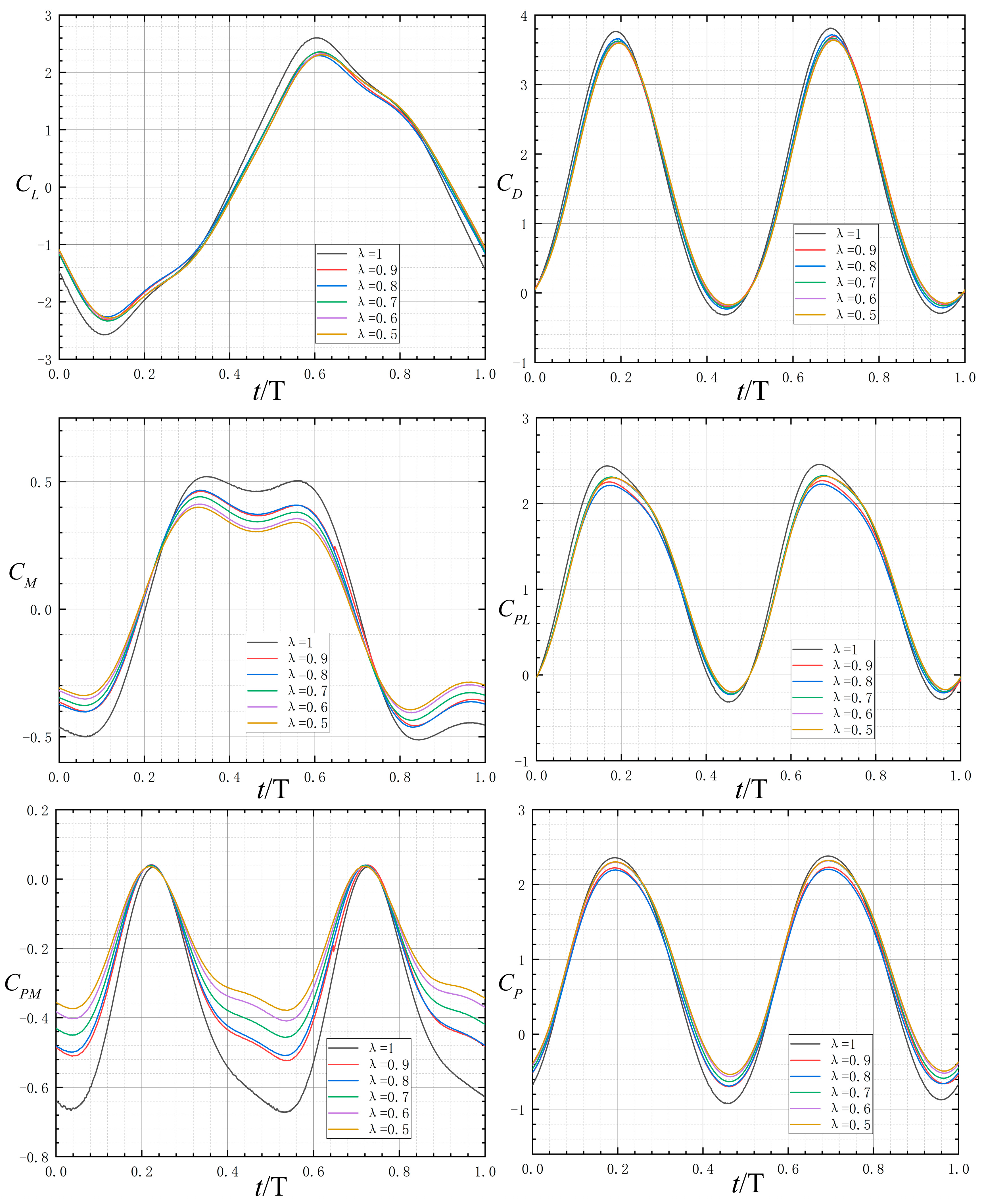
Figure 5 shows the coefficient curves of hydrofoils with different cross-sections. As can be seen from Figure 5, with the decrease in coefficient λ, the overall trend of the coefficient curves of the six hydrofoil models is consistent. The instantaneous lift coefficient $C_L$ and the instantaneous moment coefficient $C_M$ are reduced more obviously when the value of $\lambda$ is reduced from 1.0 to 0.9 at the time period of 0.4–0.7 T (i.e., near the horizontal position of the hydrofoil sinking to the horizontal position). The cross-sectional coefficient $\lambda$continues to be reduced subsequently, which has a small effect on the coefficient curves. The effect of decreasing the cross-sectional coefficient $\lambda$ on the drag coefficient $C_D$ is mainly reflected in the peak reduction.

Table 8. Comparison of calculated data with different cross-section parameters.

	${\overline{\mathit{C}}}_{\mathit{D}}$	${\widehat{\mathit{C}}}_{\mathit{L}}$	${\overline{\mathit{C}}}_{\mathit{P}\mathit{M}}$	${\overline{\mathit{C}}}_{\mathit{P}\mathit{L}}$	${\stackrel{-}{\mathit{C}}}_{\mathit{P}}$
$\lambda =1.0$	1.562	2.602	−0.371	1.175	0.804
$\lambda =0.9$	1.569	2.347	−0.296	1.145	0.849
$\lambda =0.8$	1.551	2.351	−0.278	1.141	0.864
$\lambda =0.7$	1.545	2.356	−0.257	1.148	0.891
$\lambda =0.6$	1.554	2.328	−0.219	1.143	0.922
$\lambda =0.5$	1.556	2.306	−0.211	1.148	0.944

shows the comparison of coefficients for hydrofoils with different cross-section parameters. Compared with the hydrofoil with$\lambda =1.0,$ the hydrofoil with $\lambda =0.5$ has a peak lift coefficient $C_L$ decreased by 11.4%, the peak moment coefficient $C_M$ decreased by 23.1%, the maximum drag $C_D$ decreased by 9.3%, and the average power coefficient ${\stackrel{-}{C}}_P$ increased by 17.4%. 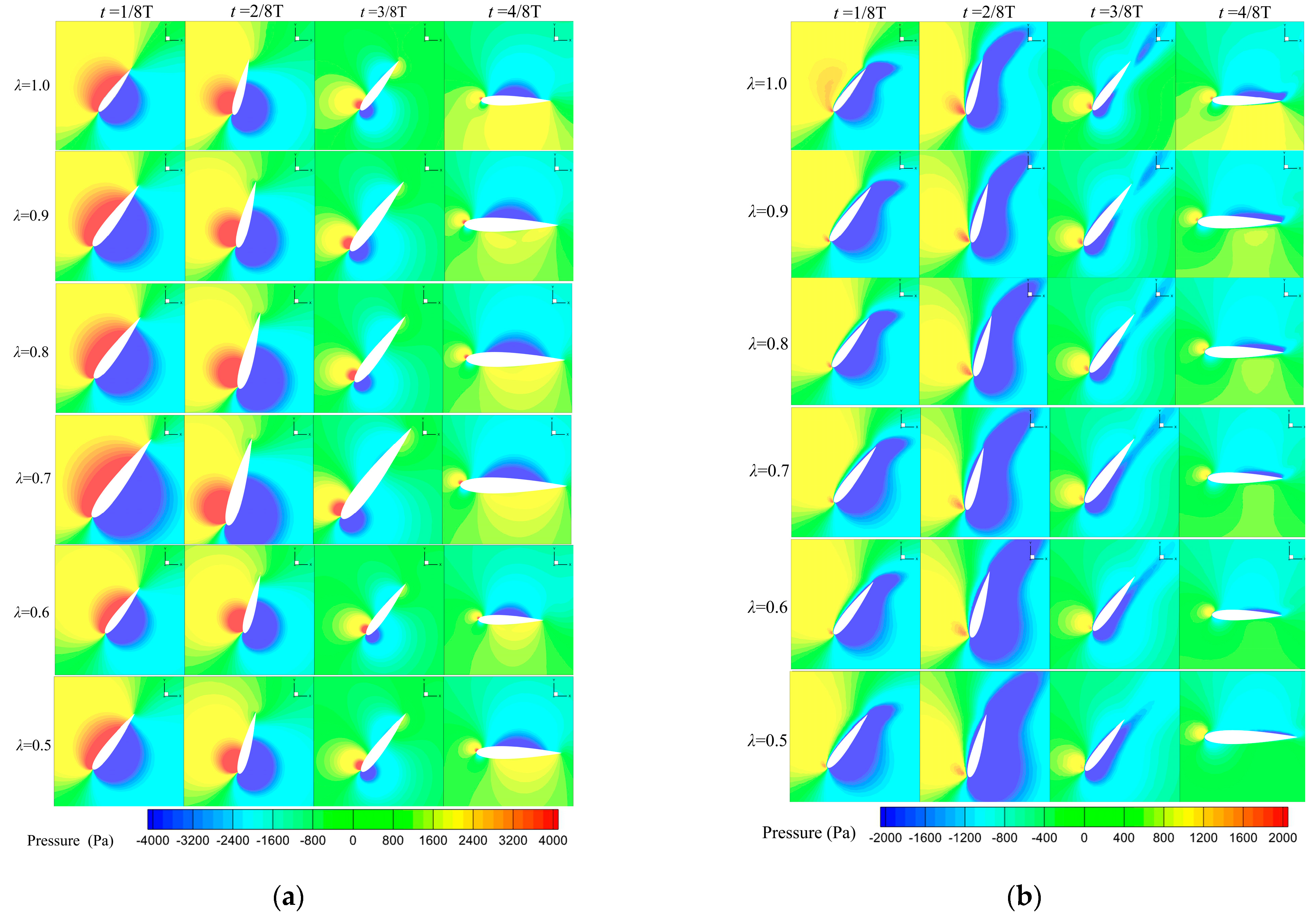Figure 6 shows the static pressure of hydrofoils with different cross-sections in a cloud diagram, which can be seen from Figure 6a. The pressure distribution at $z=0.0$ m is the same for each model, which are roughly semicircular.

This suggests that the largest difference in hydrodynamic performance around variable section hydrofoils compared to fixed-section hydrofoils is in the reduction in pitching moments, which is the main reason for the increased energy capture efficiency. This is different from previous studies about adding end plates, flexible hydrofoils, and adding trailing edges.

The hydrofoil moves from 1/8 T to 4/8 T, the high-pressure center on the upper surface gradually moves forward, the pressure at the trailing edge of the hydrofoil decreases, and the negative pressure center on the lower surface gradually decreases, and then gradually changes to a positive pressure state. From Figure 6b, it can be seen that during the downward movement of the hydrofoil, the low-pressure region appears near the upper surface at the cross-section z = 0.6 m, the low-pressure region on the lower surface of the hydrofoil is in the shape of a number “6”, and the low-pressure center near the wall decreases significantly with the decrease of $\lambda$ and approaches to the pitching axis of the hydrofoil. Combined with the hydrofoil power calculation formula, it can be seen that in one motion cycle, the direction of the lift force of the hydrofoil is the same as the direction of the velocity, the work performed by the lift force is positive, the direction of the moment is opposite to the direction of the hydrofoil rotating around the axis, and the work performed by the moment is negative. It can be seen in Figure 6 that, compared to the other time periods, the moment of the hydrofoil is larger when it is close to the pole, the power of the moment $C_{PM}$ is higher, and the reduction in the hydrofoil cross-section has a more obvious effect on the power of the moment $C_{PM}$. The effect of the reduced hydrofoil cross-section on the moment power $C_{PM}$ is more obvious. The decrease in moment power in this motion phase is larger than the decrease in lift and sink power, resulting in a higher average power coefficient of the hydrofoil and a lower average power coefficient change.

Compared to the hydrofoil with $\lambda =1.0, \lambda =0.9$ increases the average power coefficient by about 5%, and a decrease in $\lambda$ from 0.6 to 0.5 increases the average power coefficient by 2.38%. As the cross-sectional coefficient $\lambda$ decreases, the pressure center on the hydrofoil surface moves, with the high-pressure part concentrating more in the middle when $\lambda$ is small. This change affects lift and drag forces, and over-concentration may increase drag and reduce net power. Regarding tip vortex dynamics, $\lambda$ reduction shifts vortex shedding backward and increases tip vortex size and intensity, leading to more energy loss. In terms of energy extraction efficiency, while the reduction in pitching moment initially boosts the average power coefficient, the negative impacts of pressure distribution and tip vortex changes, like increased drag and vortex-related losses, gradually prevail. Consequently, the overall enhancement of the average power coefficient weakens as $\lambda$ continues to decrease. 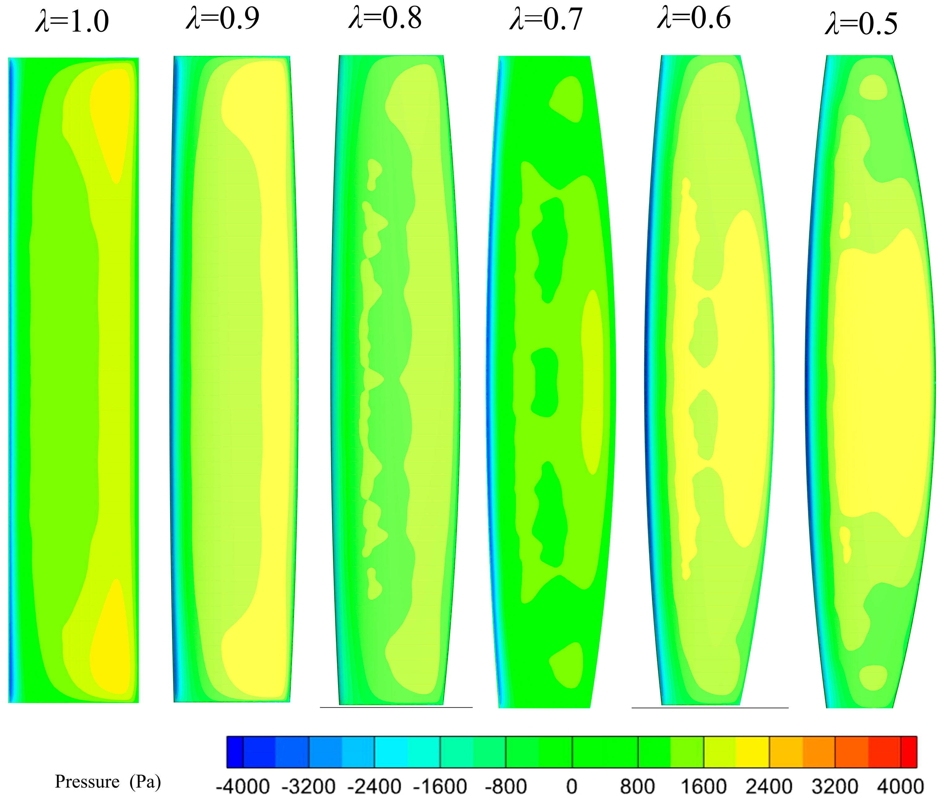Figure 7 shows the distribution of static pressure on the upper surface of the hydrofoil at t = 0.5 T. When $\lambda =1.0$, the wing end effect has a large influence, the pressure center is mainly distributed in the trailing edge of the hydrofoil and the tip portion of the hydrofoil, and the middle portion of the hydrofoil has a smaller pressure. With the decrease of $\lambda$, the pressure center on the surface of the hydrofoil is gradually divided. There are multiple high-pressure clusters, and the pressure center is gradually close to the leading edge and the middle. $\lambda =$ 0.8 and 0.7 have a small influence on the wing end effect. When $\lambda =0.5$, the high-pressure part is mainly distributed in the middle part of the hydrofoil, and the stability of the hydrofoil motion becomes worse instead.

Variable section hydrofoils can reduce the inertia of the tidal current power generation device and improve the overall efficiency of the device by improving the energy acquisition efficiency while reducing the self-weight. The reduction in pitching moment and the improvement of pressure distribution on the surface of the hydrofoils can improve the stability of the power generation device and prolong the working life, which are of significance in the research and development of the design of the power generation device.

Figure 8 shows the vortex contours at $z=0.0$ m of the hydrofoil cross-section. From Figure 8, the vortex shapes of the three hydrofoil models with$\lambda =$1.0, 0.9, and 0.5 are roughly the same at all moments, and the intensity of the vortex is slightly reduced as the value of $\lambda$ decreases. There is no obvious vortex shedding phenomenon on the upper and lower surfaces of the hydrofoils at the cross-section of $z=$0.0 m. There is no dynamic stall phenomenon, and the hydrofoils are subjected to the hydrofoil is subjected to the same water flow. 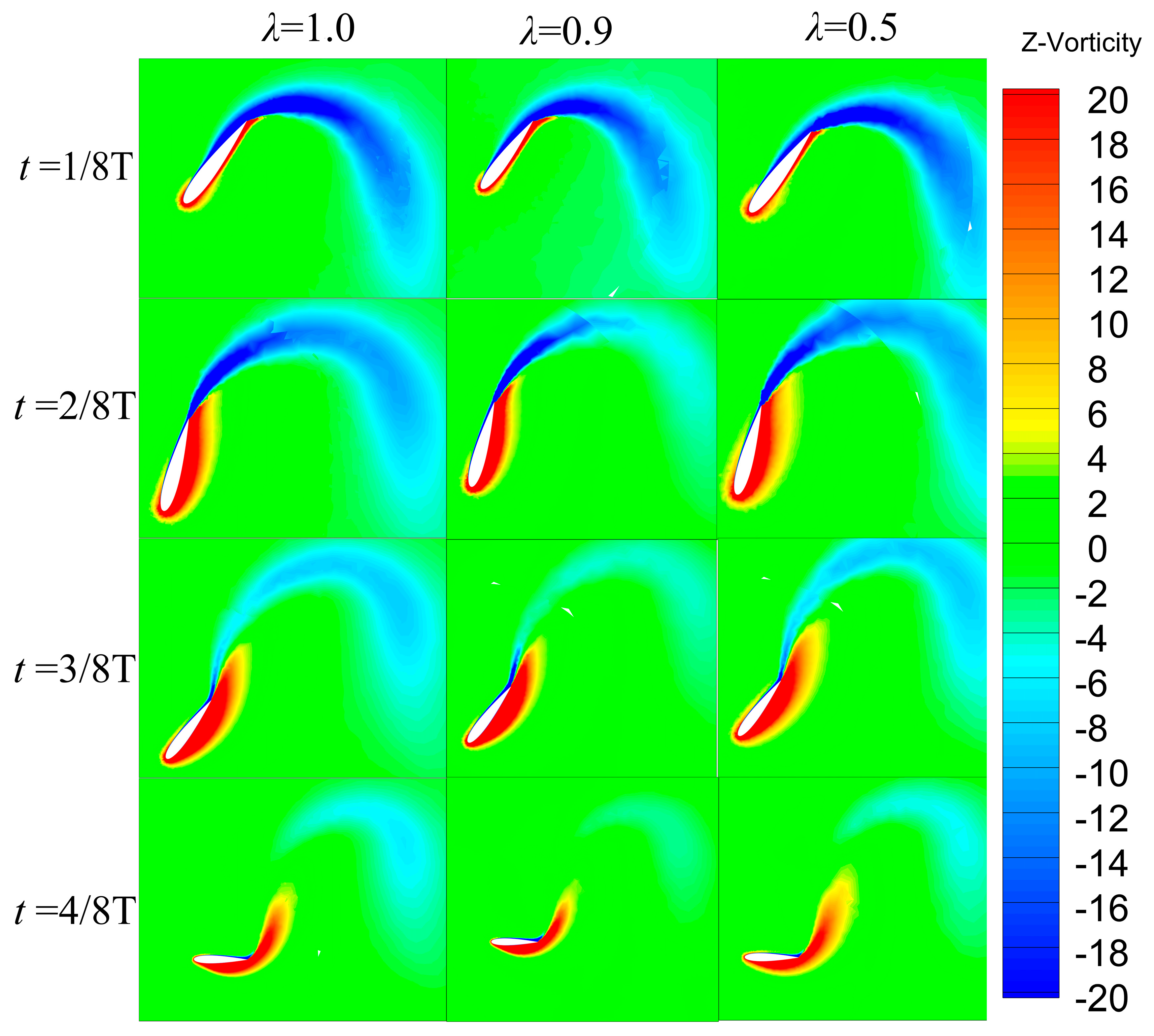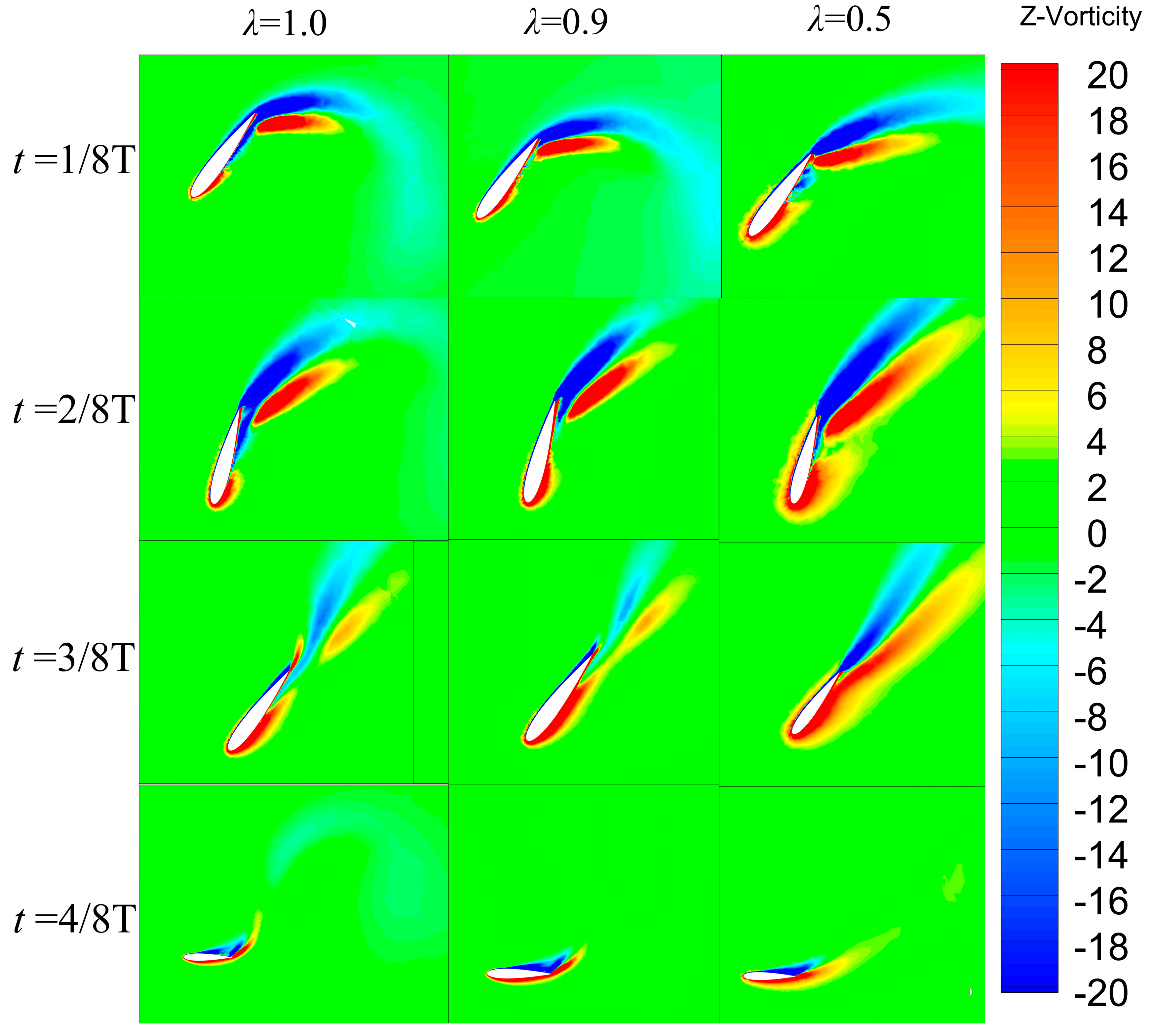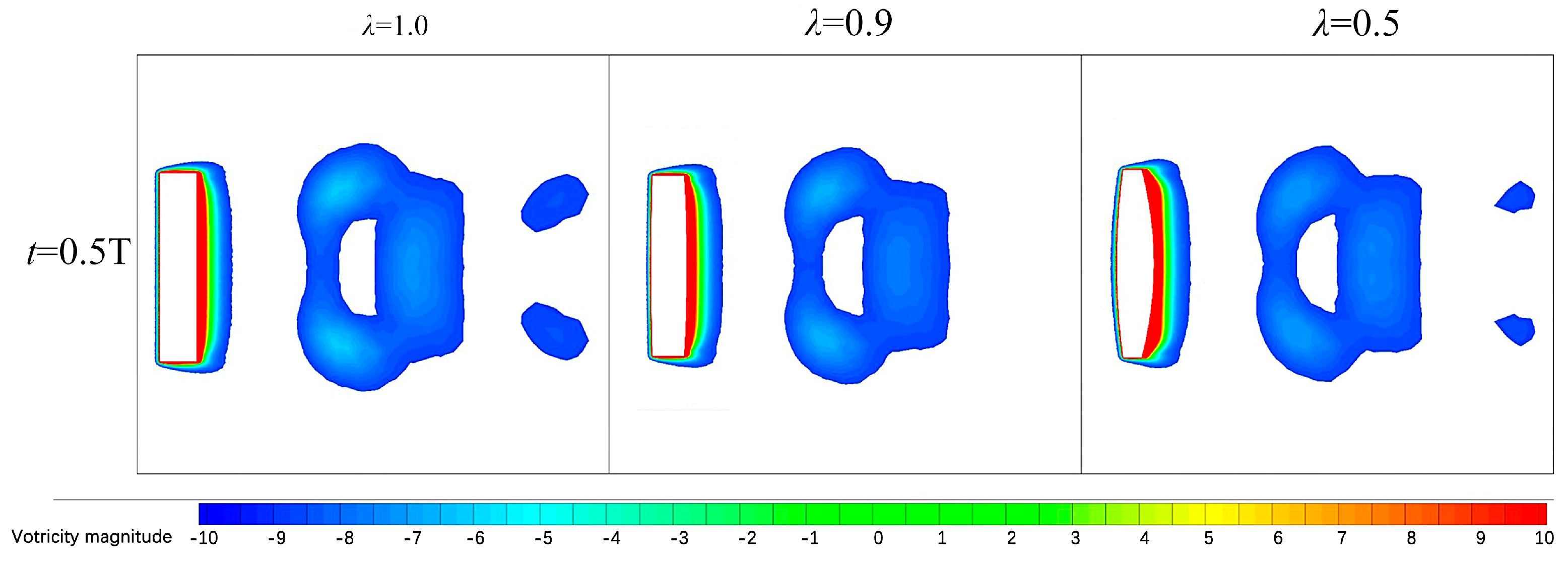Figure 9 shows the vortex contours at $\mathrm{z}=$0.6 m of the hydrofoil cross-section, and Figure 10 shows the wake vortex contours of the hydrofoil at the moment of t = 0.5 T. From Figure 9, it can be seen that the vortex of the hydrofoil model at $\lambda =$1.0 is shed along the hydrofoil wall, and as $\lambda$ decreases, the location of vortex shedding is gradually shifted backward. The three types of hydrofoils produce many tiny vortex quantities in the tips of the hydrofoils at the stage of 1/8 T to 2/8 T, and the hydrofoil wall is more prone to produce boundary separation with the increase of $\lambda$. When the vortex produced by the boundary layer separation is separated from the hydrofoil wall, the transient lift decreases, so the transient lift generated from 1/8 T to 2/8 T stage decreases. From the 1/8 T to 2/8 T stage, the hydrofoil model with $\lambda =$ 0.5 produces much larger vortex at the tip of the wing than the hydrofoil models with $\lambda =$ 1.0 and 0.9. From the vortex distribution in Figure 10, the hydrofoil cross-section decreases, the intensity of the vortex at the tail of the hydrofoil decreases slightly, and the wake vortex produced by the hydrofoil with $\lambda =$ 0.9 is smaller compared with that of $\lambda =$ 0.5. Therefore, it can be speculated that the reduction in hydrofoil cross-section reduces the tip flow and the vortex strength, reduces the hydrofoil instantaneous lifted by a small amount, and reduces the moment significantly, while too small a cross-section parameter will cause the hydrofoil to produce a larger vortex shedding, which will make the pressure overly concentrated and reduce the stability of the hydrofoil motion.

4.2. Effect of Different Dimensionless Reduced Frequencies on Hydrofoil Performance

In the process of hydrofoil motion, the angle of attack of the hydrofoil relative to the direction of the incoming flow has an important effect on the force on the hydrofoil. As the hydrofoil force is decomposed into the drag force parallel to the direction of incoming flow, the moment of rotation around the axis and the lift force perpendicular to the direction of incoming flow, the instantaneous effective angle of attack of the hydrofoil is not the pitch angle, and the effective angle of attack of the hydrofoil at this point in time is calculated by the following formula [32]:

$$\begin{array}{c}{\alpha }_{eff}\left(t\right)=\mathit{arctan}\left[-V_y\left(t\right)/U_{\infty }\right]-\theta \left(t\right).\end{array}$$

(20)

Hydrofoil lifting and sinking motion of the speed difference is not large, cannot be ignored, at this time the hydrofoil’s equivalent incoming velocity for the water velocity and lifting and sinking speed of the synthesis, the equivalent incoming velocity is defined as follows [10]:

$$U_t=\sqrt{U_{\infty }^2+{v\left(t\right)}^2}.$$

(21)

In the non-constant flow, it is not convenient to determine the relationship between the hydrodynamic performance of the hydrofoil and the angle of attack by the available experimental data. From the above, it is known that reducing the cross-section parameter λ can appropriately increase the average power, but continuing to reduce λ will reduce the stability of the hydrofoil movement frequency. Then, we try to select the variable cross-section airfoil with $\lambda =$ 0.5, the lift and sinking amplitude h is selected to be c, the pitch angle is 75°, and the dimensionless reduced frequency $f^{*}=$ 0.12, 0.14, 0.16, and study the relationship between the performance of the hydrofoil designed and the reduced frequency.

Table 9. Comparison of calculated coefficients for different dimensionless reduced frequencies.

${\mathit{f}}^{\mathit{*}}$	${\overline{\mathit{C}}}_{\mathit{D}}$	${\widehat{\mathit{C}}}_{\mathit{L}}$	${\overline{\mathit{C}}}_{\mathit{P}\mathit{M}}$	${\overline{\mathit{C}}}_{\mathit{P}\mathit{L}}$	${\overline{\mathit{C}}}_{\mathit{P}}$
0.12	1.564	2.230	−0.110	1.025	0.905
0.14	1.556	2.306	−0.211	1.148	0.944
0.16	1.559	2.563	−0.311	1.251	0.939

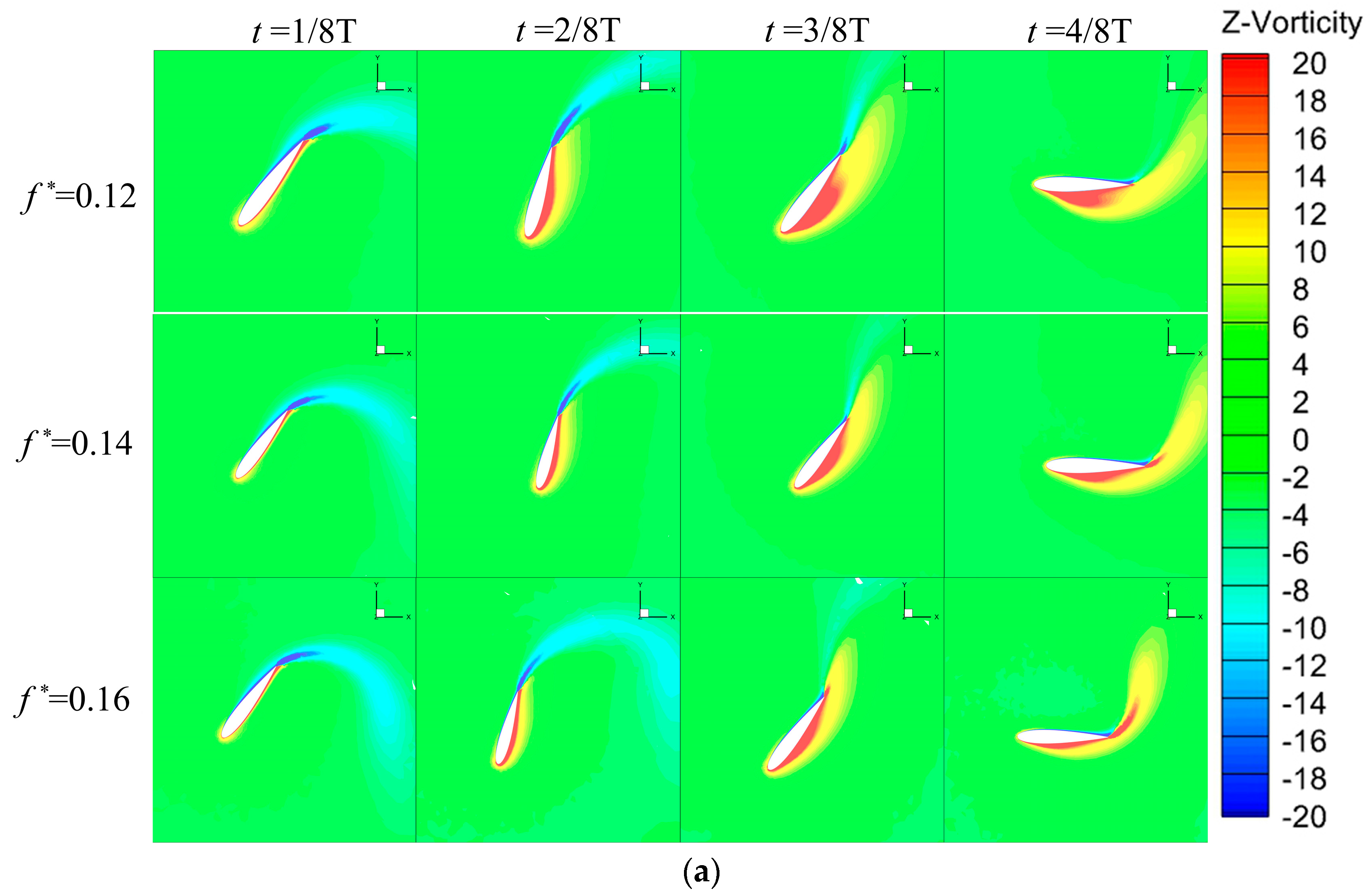
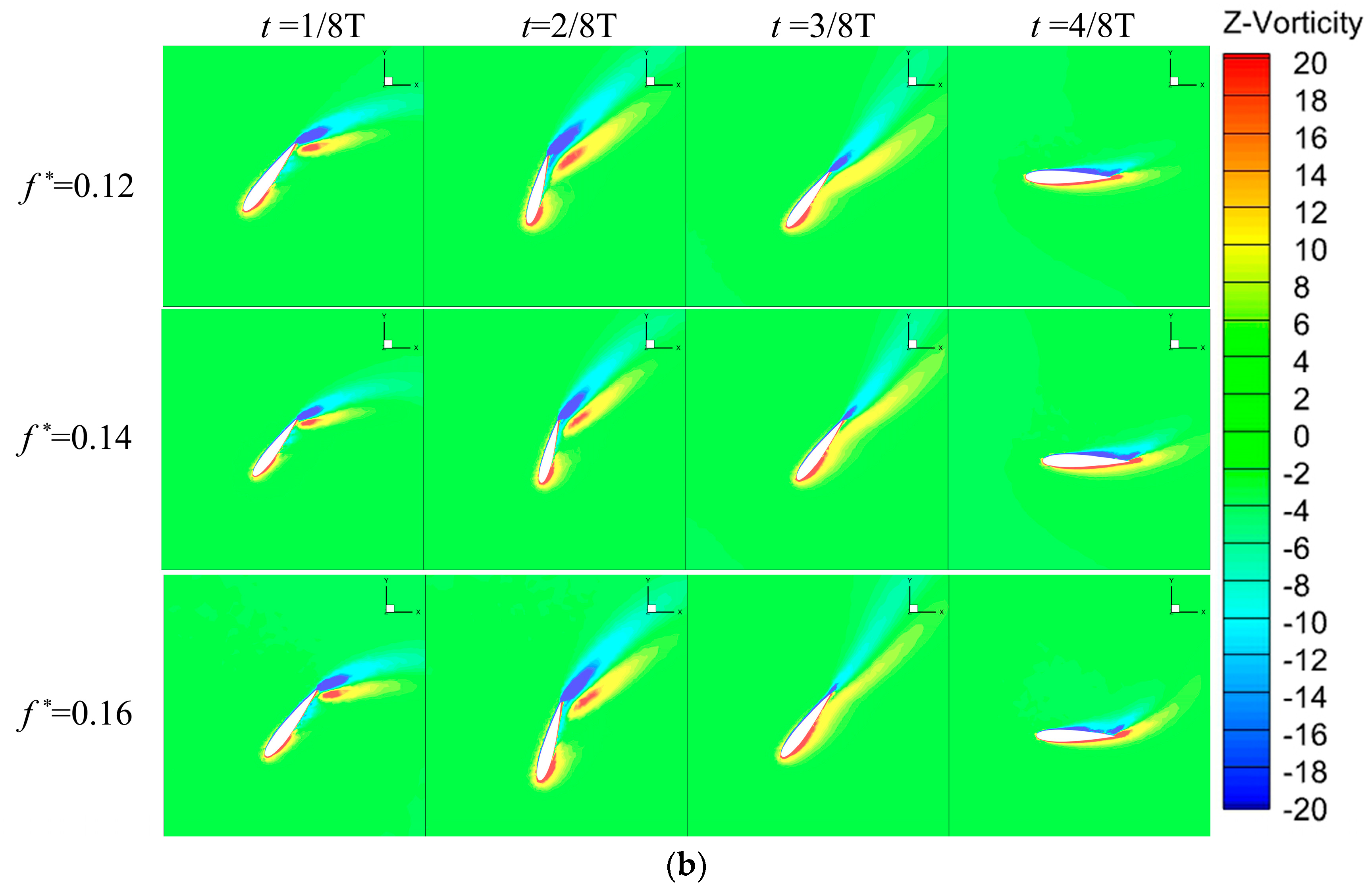
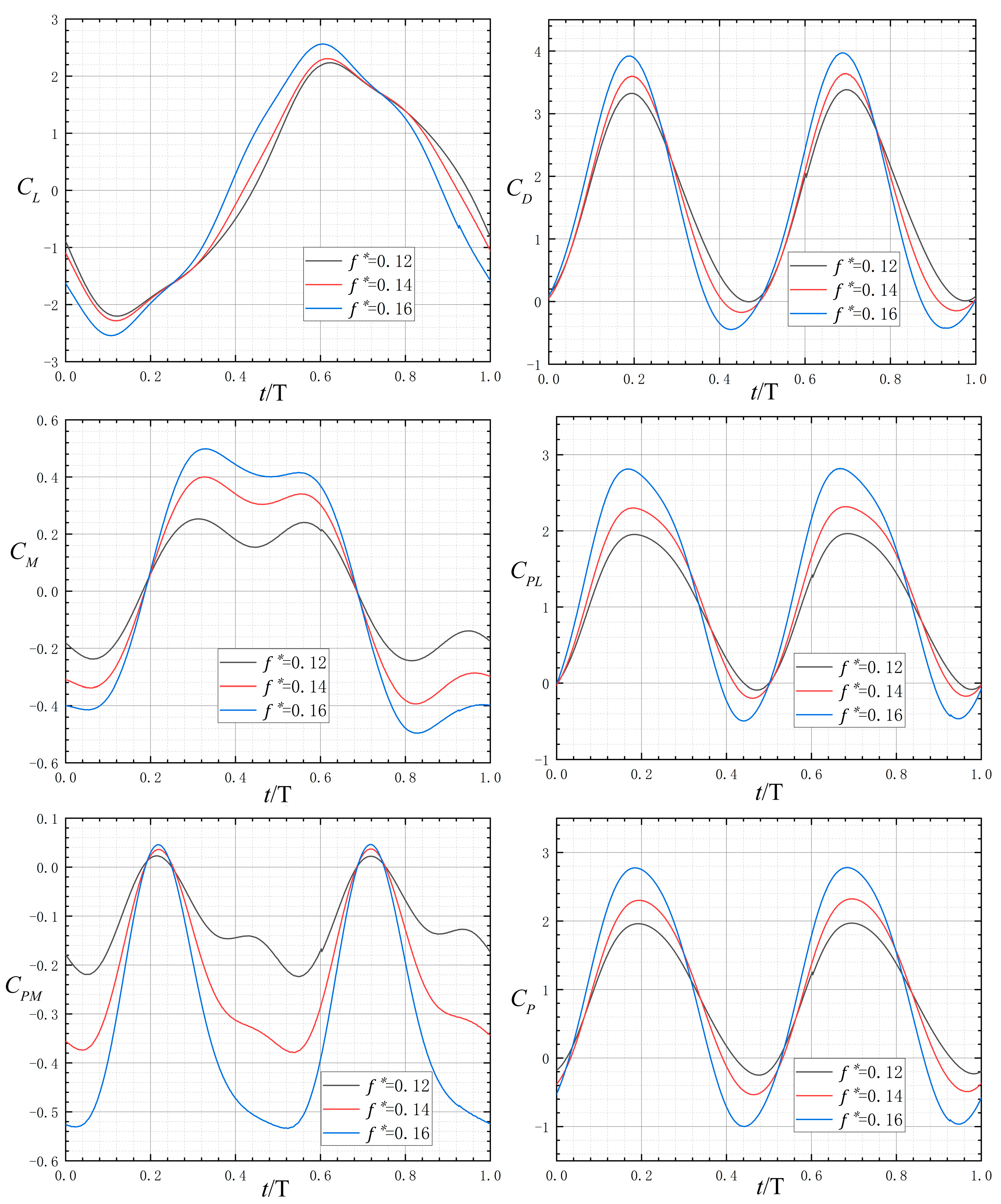
shows the comparison of the coefficients under different reduced frequencies, Figure 10 shows the dimensionless reduced frequency hydrofoil’s vorticity contours, and Figure 11 shows the coefficient curves under different reduced frequencies.

From Figure 12, the dimensionless reduced frequency $f^{\mathrm{*}}$ has a great influence on the peak value of each curve of coefficients, and the higher the reduced frequency, the larger the peak value. Combined with the data in Table 9, the increase in dimensionless reduced frequency $f^{\mathrm{*}}$ has little effect on the average resistance, the average lift power increases while the average moment power increases, and the average power first increases and then decreases due to the negative value of the work performed by the moment. From Figure 11, under three dimensionless reduced frequencies, there is no obvious phenomenon of vortex shedding caused by boundary layer separation on the hydrofoil wall, and from the stage of 3/8 T to 4/8 T, the vortex at the mid-section of the hydrofoil becomes smaller when the reduced frequency $f^{\mathrm{*}}$ is increased. Therefore, continuing to increase the dimensionless reduced frequency does not improve the average power of the hydrofoil, which is higher at $f^{\mathrm{*}}=$ 0.14.

5. Conclusions

In this study, we combined the characteristics of flat and elliptical wings and used parabolic fitting to the leading and trailing edges of the hydrofoil to obtain six hydrofoils with different sizes of section. We used the S-A Turbulence Model to simulate the pitching and ascending and descending motion of hydrofoil to obtain the coefficient curves of the models, and obtained the following conclusions by analyzing the vorticity and pressure distributions of the hydrofoils:

• The designed hydrofoil effectively reduces the peaks of the drag coefficient and moment coefficient of the hydrofoil, enhances the stability of the hydrofoil to the hydrofoil motion, and provides reference for the optimal design of the hydrofoil.
• By comparing the flat wing, it is found that by reducing the hydrofoil end surface will cut down the peaks of the instantaneous lift coefficient, instantaneous drag coefficient, and instantaneous moment coefficient curves, where the instantaneous moment coefficient reduction is greater than the instantaneous lift coefficient, and therefore the average power is higher.
• Under the same basin environment and working conditions, the selection of hydrofoils with smaller cross-sectional coefficient $\lambda$ can improve the hydrofoil surface pressure distribution and make the hydrofoil motion more stable, but the cross-sectional coefficient $\lambda$is too small will make the hydrofoil surface pressure too concentrated and reduce the stability of hydrofoil motion.
• By comparing the average power at different dimensionless reduced frequencies, it is obtained that for $\lambda =$ 0.5 there is a higher average power coefficient of 0.944 at the reduced frequency $f^{*}=$ 0.14.

This work will help to enrich the design of hydrofoil structures and increase the power of hydrofoil devices used to capture tidal energy. Future work should investigate the real hydrodynamic performance of variable section hydrofoils by conducting underwater tests in realistic conditions of the sea.

References

1. Daoxian, Y. Environmental Geology: Proceedings of the 30th International Geological Congress; CRC Press: Boca Raton, FL, USA, 1997; Volume 24. [Google Scholar]
2. Yin, H.; Wang, Y.; Sun, W.; Wang, L. Fault diagnosis of hydraulic system based on D-S evidence theory and SVM. Int. J. Hydromechatronics 2024, 7, 1–15. [Google Scholar] [CrossRef]
3. Mckineey, W.; DeLaurier, J. Thewingmill an oscillating-wing wingmill. J. Energy 1981, 5, 109–115. [Google Scholar] [CrossRef]
4. Kinsey, T.; Dumas, G. Computational Fluid Dynamics Analysis of a Hydrokinetic Turbine Based on Oscillating Hydrofoils. J. Fluids Eng. 2012, 134, 021104. [Google Scholar] [CrossRef]
5. Zeiner-Gundersen, D.H. A novel flexible foil vertical axis turbine for river, ocean, and tidal applications. Appl. Energy 2015, 151, 60–66. [Google Scholar] [CrossRef]
6. Liu, Z.; Qu, H.; Song, X.; Chen, Z.; Ni, H. Energy-harvesting performance of tandem coupled-pitching hydrofoils under the semi-activated mode: An experimental study. Energy 2023, 279, 128060. [Google Scholar] [CrossRef]
7. Pernod, L.; Ducoin, A.; Sourne, H.L.; Astolfi, J.-A.; Casari, P. Experimental and numerical investigation of the fluid-structure interaction on a flexible composite hydrofoil under viscous flows. Ocean. Eng. 2019, 194, 106647. [Google Scholar] [CrossRef]
8. Zeng, Y.S.; Yao, Z.F.; Zhou, P.J.; Wang, F.J.; Hong, Y.P. Numerical investigation into the effect of the trailing edge shape on added mass and hydrodynamic damping for a hydrofoil. J. Fluids Struct. 2019, 88, 167–184. [Google Scholar] [CrossRef]
9. Xiao, Q.; Zhu, Q. A review on flow energy harvesters based on flapping foils. J. Fluids Struct. 2014, 46, 174–191. [Google Scholar] [CrossRef]
10. Wu, X.; Zhang, X.; Tian, X.; Li, X.; Lu, W. A review on fluid dynamics of flapping foils. Ocean. Eng. 2020, 195, 106712. [Google Scholar] [CrossRef]
11. Zhang, Y.; Wang, Y.; Xie, Y.; Sun, G.; Han, J. Effects of flexibility on energy extraction performance of an oscillating hydrofoil under a semi-activated mode. Energy 2022, 242, 122940. [Google Scholar] [CrossRef]
12. Le, T.Q.; Ko, J.H. Effect of hydrofoil flexibility on the power extraction of a flapping tidal generator via two- and three-dimensional flow simulations. Renew. Energy 2015, 80, 275–285. [Google Scholar] [CrossRef]
13. Liu, Z.; Qu, H.; Shi, H. Performance evaluation and enhancement of a semi-activated flapping hydrofoil in shear flows. Energy 2019, 189, 116255. [Google Scholar] [CrossRef]
14. Xiao, Q.; Liao, W.; Yang, S.; Peng, Y. How motion trajectory affects energy extraction performance of a biomimic energy generator with an oscillating foil. Renew. Energy 2012, 37, 61–75. [Google Scholar] [CrossRef]
15. Custodio, D.; Henoch, C.; Johari, H. Cavitation on hydrofoils with leading edge protuberances. Ocean. Eng. 2018, 162, 196–208. [Google Scholar] [CrossRef]
16. Hu, J.; Xiao, Q. Three-dimensional effects on the translational locomotion of a passive heaving wing. J. Fluids Struct. 2014, 46, 77–88. [Google Scholar] [CrossRef]
17. Zhang, L. Aerodynamics Analysis of Space Shuttle, 1st ed.; Guo Fang Gong Ye Chu Ban She: Beijing, China, 2009. [Google Scholar]
18. Pan, Z.; Guan, J.; Yang, X.; Guo, A.; Wang, X. 3D profile-based pothole segmentation and quantification. Int. J. Hydromechatronics 2024, 7, 16–30. [Google Scholar] [CrossRef]
19. Meng, Y.-S.; Yan, L.; Huang, W. Structural design and analysis of a composite wing with high aspect ratio. J. Zhejiang Univ.-Sci. A 2019, 20, 781–793. [Google Scholar] [CrossRef]
20. Xiangru, C. Theoretical and Experimental Study on the Leading-edge Tubercle of Three-dimensional Airfoil. Harbin Eng. Univ. 2016, 37, 248–253. [Google Scholar]
21. Zhi-jun, Z.; Tian-ge, L.; Teng-fei, S.; Ji-yu, S. Study on Laminar Flow Separation of Elliptic Airfoils at Low Reynolds Numbers. J. Northeast. Univ. 2022, 43, 1753–1760. [Google Scholar]
22. Ning, H.; Qian, S.; Zhou, T. Applications of level set method in computational fhuid a review. Int. J. Hydromechatronics 2023, 6, 1–33. [Google Scholar] [CrossRef]
23. Hong, C.; Oiao, S.; Shah, A.A. Inflence of oil temperature on pressure distribution and flow force of valve core. Int. J. Hydromechatronics 2023, 6, 342–358. [Google Scholar] [CrossRef]
24. Kanitmozhi, T.; Jmarani, S. A comparative study of energy-efficient chustering protocols for WSN-internet-of things. Int. J. Hydromechatronics 2023, 2, 177–196. [Google Scholar] [CrossRef]
25. Liu, W.; Wang, X.; Mi, K. The Numerical Research on Flow Mechanism of Forward-Swept Wing and Backward-Swept Wing Configurations. J. Air Force Eng. Univ. 2008, 6, 11–15. [Google Scholar]
26. Hover, F.S.; Haugsdal, Ø.; Triantafyllou, M.S. Effect of angle of attack profiles in flapping foil propulsion. J. Fluids Struct. 2004, 19, 37–47. [Google Scholar] [CrossRef]
27. Zhu, Q.; Peng, Z. Mode coupling and flow energy harvesting by a flapping foil. Phys. Fluids 2009, 21, 033601. [Google Scholar] [CrossRef]
28. Shahsavari, A.; Nejat, A.; Climent, E.; Chini, S.F. Unexpected trends of lift for hydrofoils with superhydrophobic coating. Eur. J. Mech. B/Fluids 2023, 101, 219–226. [Google Scholar] [CrossRef]
29. Liu, Y.; Tan, L. Method of C groove on vortex suppression and energy performance improvement for a NACA0009 hydrofoil with tip clearance in tidal energy. Energy 2018, 155, 448–461. [Google Scholar] [CrossRef]
30. Heathcote, S.; Wang, Z.; Gursul, I. Effect of spanwise flexibility on flapping wing propulsion. J. Fluids Struct. 2008, 24, 183–199. [Google Scholar] [CrossRef]
31. Jin, S.; Peng, H.; Qiu, W.; Hunter, R.; Thompson, S. Numerical simulation of planing hull motions in calm water and waves with overset grid. Ocean. Eng. 2023, 287, 115858. [Google Scholar] [CrossRef]
32. Kinsey, T.; Dumas, G. Three-Dimensional Effects on an Oscillating-Foil Hydrokinetic Turbine. J. Fluids Eng. 2012, 134, 071105. [Google Scholar] [CrossRef]
Figure 1. Display of different wing profiles.
Actuators 14 00217 g001
Figure 2. Hydrofoil motion model and force analysis.
Actuators 14 00217 g002
Figure 3. Designed hydrofoil geometry.
Actuators 14 00217 g003
Figure 4. Watershed model and meshing.
Actuators 14 00217 g004
Figure 5. Coefficient profiles of hydrofoils with different cross-sectional coefficient parameters.
Actuators 14 00217 g005
Figure 6. Static pressure contours for hydrofoils with different cross-sectional coefficients (a) z = 0.0 m, (b) z =0.6 m.
Actuators 14 00217 g006
Figure 7. Contours of static pressure on the upper surface of hydrofoil at t =0.5 T.
Actuators 14 00217 g007
Figure 8. Contours of vorticity at z = 0.0 m of hydrofoil cross-section.
Actuators 14 00217 g008
Figure 9. Contours of vorticity at z = 0.6 m of hydrofoil cross-section.
Actuators 14 00217 g009
Figure 10. Tail vortex contours of hydrofoils with different cross-sections at t = 0.5 T.
Actuators 14 00217 g010
Figure 11. Vorticity plots of hydrofoils at different dimensionless reduced frequencies f * , (a) z = 0.0 m, (b) z = 0.6 m.
Actuators 14 00217 g011aActuators 14 00217 g011b
Figure 12. Coefficient curves for different dimensionless reduced frequencies f * .
Actuators 14 00217 g012