Non-Singular Fast Sliding Mode Control of Robot Manipulators Based on Integrated Dynamic Compensation

Abstract

In order to realize the problem of tracking control of the trajectory of robot manipulators under variable load conditions, this paper proposes a non-singular fast terminal sliding mode tracking control design for robot manipulators based on integrated dynamic compensation. First, in the model, the friction torque under the influence of speed is considered while combined with the joint torque estimation for integrated dynamic compensation. Second, a novel non-singular fast terminal sliding mode controller is proposed, which helps to overcome the singularity problem and has been analyzed for stability using the Lyapunov method. Finally, trajectory tracking experiments are conducted on an experimental platform and compared with the PID algorithm, demonstrating the superior control performance of the proposed algorithm.

1. Introduction

In the process of modern industrial automation and intelligent manufacturing, collaborative robot manipulators play a central role, and their trajectory tracking accuracy is directly related to the production efficiency, product quality, and operational safety. However, robot manipulator systems face challenges such as modeling errors, parameter uncertainties, and external disturbances. Achieving high-precision trajectory tracking control has been a challenging topic.

In order to improve the trajectory tracking control accuracy, researchers have proposed numerous advanced control algorithms, such as PID control [1,2], sliding mode control [3,4], adaptive control [5,6], iterative learning control [7,8], fuzzy control [9,10], and neural network control [11,12]. The common PID control has a simple structure, which is insensitive to parameter changes. Moreover, it cannot automatically adjust the parameters according to variable load conditions. Both fuzzy control and neural network control require the design of numerous parameters, which leads to a large computational load and high difficulty in engineering applications. Although iterative learning control, reinforcement learning, and neural network control do not rely on accurate models and have strong adaptability, they require a large amount of training data and may have generalization problems. In contrast, sliding mode control, with the advantages of handling uncertain parameters, fast response, and strong robustness, is widely applied in the fields of nonlinear and robust control [13].

However, traditional sliding mode control is not perfect. The initial SMC has two drawbacks: first, it is slower than the traditional linear SMC to converge to the equilibrium point when the system state is far away from the equilibrium point, and second, it suffers from the singularity problem. In order to ensure that the tracking error on the sliding mode surface can converge in a finite time, a nonlinear function is introduced into the sliding mode control, so researchers proposed the terminal siding mode control [14]. To avoid the issue of singularity, where the control law value tends to infinity as the system state variables approach zero, researchers have proposed the non-singular terminal sliding mode control algorithm [15,16]. To solve the above two problems at the same time, the designers proposed the non-singular fast terminal sliding mode control [17,18].

Load estimation is an important issue in robot manipulator control. Estimating the load contributes to improving the control accuracy of robot manipulators. Common methods used for the load estimation of robot manipulators include extended state observer [19,20], disturbance observer [21,22], and time-delay estimation [23,24]. The existing load estimation methods each have their own limitations. Disturbance observer depends on the system model. The observer parameters are difficult to adjust, requiring a lot of simulations and experiments for testing. Time-delay estimation is model-free but requires a large amount of data and has high computational complexity. Estimating the external force by utilizing the position information from the motor side and the joint side in combination with the harmonic drive model, and compensating for the estimated value of joint load torque in the robot manipulator model, provides a new approach for load estimation [25].

In view of the above discussion, this paper proposes a non-singular fast terminal sliding mode controller for robot manipulators based on integrated dynamic compensation of the friction and joint torque. Considering the effect of speed on friction, the model is compensated for friction. Meanwhile, the compliance model of the harmonic reducer’s flexible wheel torsional torque is represented by a cubic polynomial to estimate the torque, achieving comprehensive dynamic compensation. Finally, a novel sliding surface combined with adaptive dynamic gain adjustment is proposed to enhance the accuracy of the robot manipulators’ trajectory tracking control.

Section 2 of this paper focuses on the dynamic modeling of the robot and the integrated dynamic compensation modeling of the friction and joint torque. Section 3 proposes a non-singular fast terminal sliding mode tracking control design for robot manipulators based on integrated dynamic compensation. The stability of the controller is proven using the Lyapunov method. Section 4 describes the experimental setup and results. Section 5 summarizes the research achievements and outlines future work.

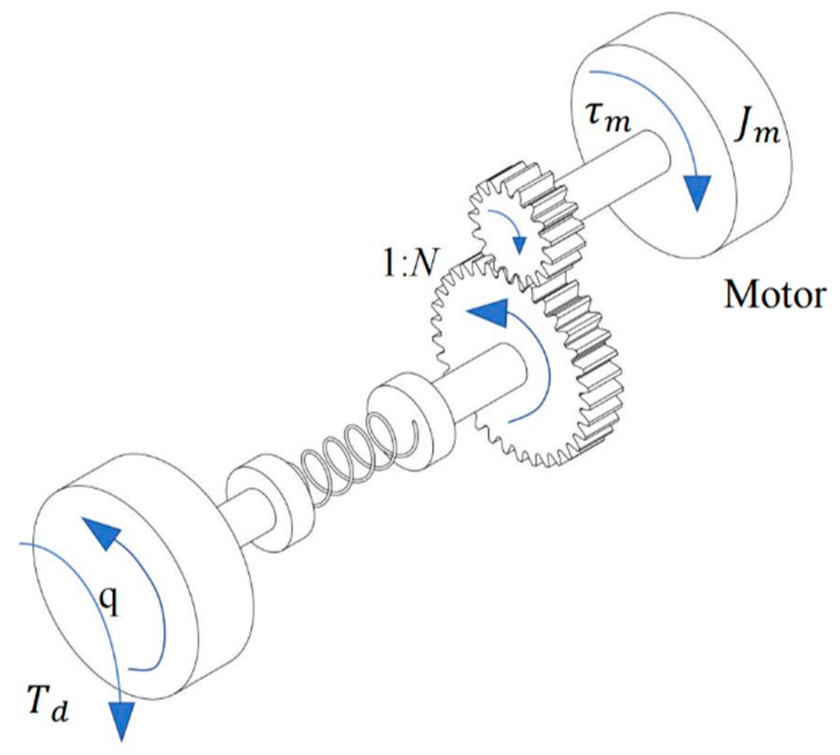
2. Robot Dynamics

2.1. Dynamics of n-DOF Robot Manipulators

As shown in Figure 1, the dynamic equation for an n-DOF robot manipulator can be expressed as follows:

$$N{\tau }_m=N^2{J}_m\ddot{q}+N{\tau }_{fm}+M\left(q\right)\ddot{q}+C\left(q,\dot{q}\right)\dot{q}+G\left(q\right)+{\tau }_{fl}+{\tau }_d,$$

(1)

where $J_m$ is the inertia of the motor; ${\tau }_m$ and ${\tau }_{fm}$ denote the motor torque vectors and the friction torque of the motor-side; $M(q)$, $C(q,\dot{q})$, $G(q)$ are the inertia matrix, Coriolis (centripetal) matrix, and gravity matrix of the robot manipulators; $q$ denotes the angular displacement vectors of the load-side; $\ddot{q}$ and $\dot{q}$ are the angular acceleration vectors and angular velocity vectors of the load-side, respectively; ${\tau }_s$, ${\tau }_{fl}$ and ${\tau }_d$ are the flex-wheel torsion torque, friction torque of the load-side, and the disturbance; and $N$ is the reduction ratio.

Simplify Equation (1) to:

$$T_M=J\ddot{q}+T_{\mathrm{f}}+T_{\mathrm{d}},$$

(2)

where $T_M$ is the output torque produced by the motor, $J$ is the moment of inertia of the motor-side converted to the load-side, and $T_{\mathrm{f}}$, $T_{\mathrm{d}}$ denote the total frictional torque and total disturbance torque, respectively.

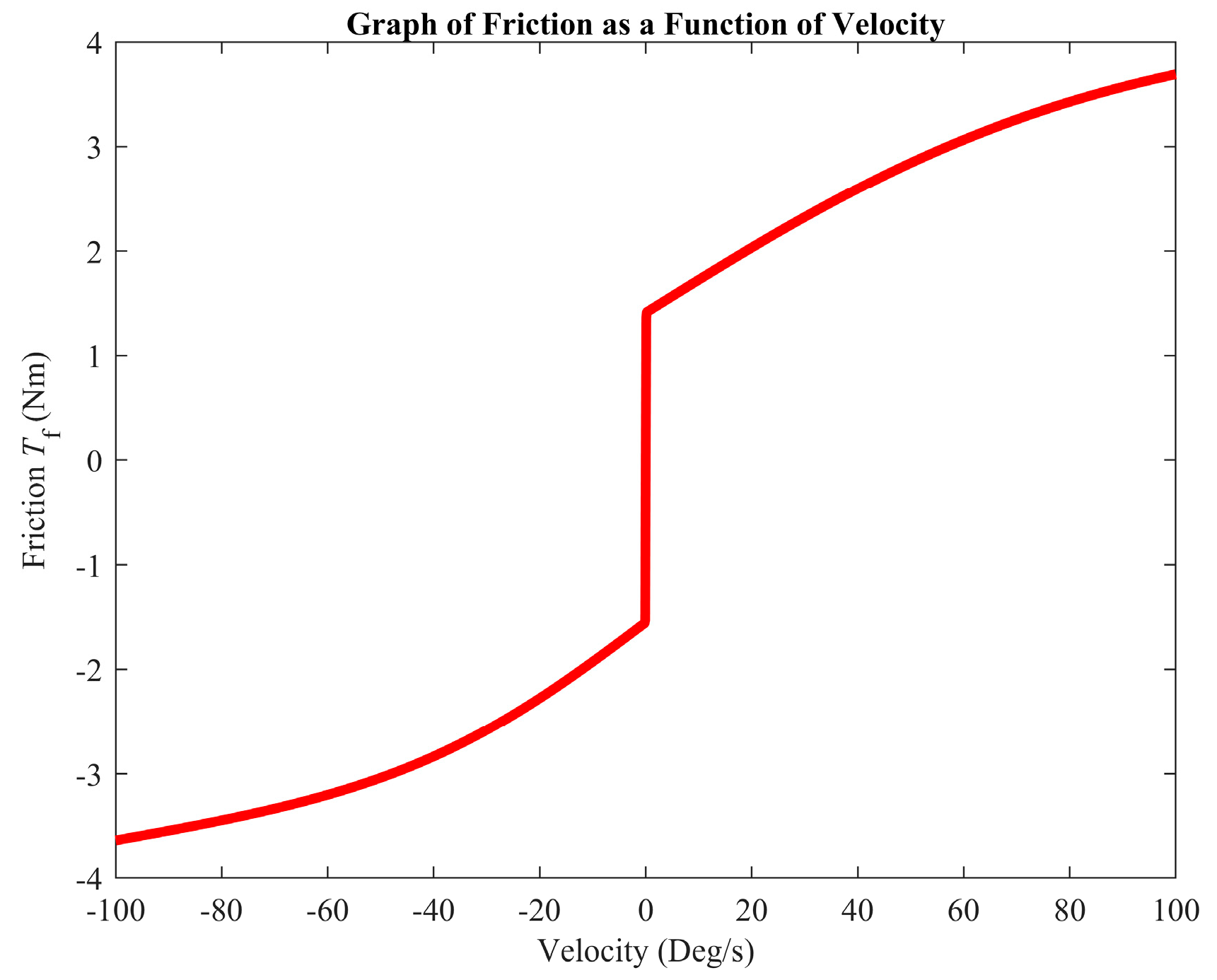
2.2. Integrated Friction and Joint Torque Dynamic Compensation

The integrated dynamic compensation includes friction compensation and joint torque compensation.

Firstly, friction modeling is conducted. When the robot manipulators are not loaded, static friction (such as Coulomb friction) can cause errors in the joints during startup or stoppage. Through friction compensation, these errors can be effectively reduced, thereby improving the positioning accuracy. During motion, dynamic friction (such as viscous friction) can affect the tracking accuracy of the velocity and acceleration. Friction compensation can mitigate these effects, making the motion of the robot manipulators smoother and reducing the velocity fluctuations. Considering the influence of velocity on friction torque [26,27,28], the following friction model is established:

$${\widehat{T}}_{\mathrm{f}}=a_1\left(tanh\left(a_2·\dot{q}\right)-tanh\left(a_3·\dot{q}\right)\right)+a_{4}tanh\left(a_5·\dot{q}\right)+a_6·\dot{q},$$

(3)

where ${\widehat{T}}_{\mathrm{f}}$ represents the estimated total frictional torque and $a_1$, $a_2$, $a_3$, $a_4$, $a_5$, $a_6$ are friction coefficients related to velocity.

During the experimental process, tests were conducted on different speeds for both clockwise and counterclockwise rotations to obtain the corresponding friction torque data. The least squares method was then applied to fit these data, resulting in the graph shown in Figure 2, which illustrates the variation of the friction torque with the velocity.

Table 1. Friction parameter results for clockwise rotation.

${\mathit{a}}_1$	${\mathit{a}}_2$	${\mathit{a}}_3$	${\mathit{a}}_4$	${\mathit{a}}_5$	${\mathit{a}}_6$
−1.477	−0.02592	−7.865	−2.967	−4.188	0.01478

and

Table 2. Friction parameter results for counterclockwise rotation.

${\mathit{a}}_1$	${\mathit{a}}_2$	${\mathit{a}}_3$	${\mathit{a}}_4$	${\mathit{a}}_5$	${\mathit{a}}_6$
−1.218	18.28	0.02605	2.692	18.62	0.01876

present the corresponding values of the friction coefficients.

The following is the joint torque compensation. Due to the material deformation during transmission, the flexible robot manipulators experience torque-induced torsional errors:

$$∆\theta =q-{\displaystyle \frac{\theta }{N}}.$$

(4)

Since the motion error varies periodically with the absolute angular velocity on the output side [29], the errors generated during forward and reverse rotation need to be identified. The motion error is defined as follows:

$$\vartheta =\left\{\begin{array}{c}\sum A_{+}sin({\omega }_{+}q+{\phi }_{+})\dot{q}\ge 0\\ \sum A_{-}sin({\omega }_{-}q+{\phi }_{-})\dot{q}<0\end{array}\right.,$$

(5)

where $A_{+}$ and $A_{-}$ represent the amplitudes of the motion errors during forward and reverse rotation, respectively; ${\omega }_{+}$ and ${\omega }_{-}$ represent the angular velocities of the errors during forward and reverse rotation, respectively; and ${\phi }_{+}$ and ${\phi }_{-}$ represent the phases of the errors during forward and reverse rotation, respectively.

The torsional torque of the flexible wheel based on the flexibility model of the harmonic drive can be represented by a cubic polynomial [30], thereby obtaining the relationship between the estimated torque and the torsion angle.

$${\tau }_s=K_{s1}\left(∆\theta -\vartheta \right)+K_{s2}{\left(∆\theta -\vartheta \right)}^3,$$

(6)

where ${\tau }_s$ represents the torsional torque of the flexspline, and $K_{s1}$ and $K_{s2}$ represent the nonlinear stiffness of the flexspline at the node.

Based on the influence of the friction and disturbance torques discussed above on the control of the robot manipulators, we define $\mathrm{T}$ as the integrated compensation torque. Meanwhile, the total external disturbance torque ${\mathrm{T}}_{\mathrm{d}}$ is estimated through the torsional torque of the flexspline ${\mathsf{\tau }}_{\mathrm{s}}$. Therefore, the integrated dynamic compensation torque is estimated as follows:

$$\widehat{T}={\widehat{T}}_{\mathrm{f}}+{\widehat{T}}_{\mathrm{d}},$$

(7)

where $\widehat{T}$ represents the estimated integrated compensation torque and ${\widehat{T}}_{\mathrm{d}}$ denotes the total disturbance torque.

By varying the magnitude of the load torque, different torsion angles and estimated torques can be obtained through experiments. Using the least squares method to fit the relationship between them, the joint torque estimation parameters are obtained as $K_{s1}$ = −0.1005 and $K_{s2}$ = −2.6 × 10⁻⁶.

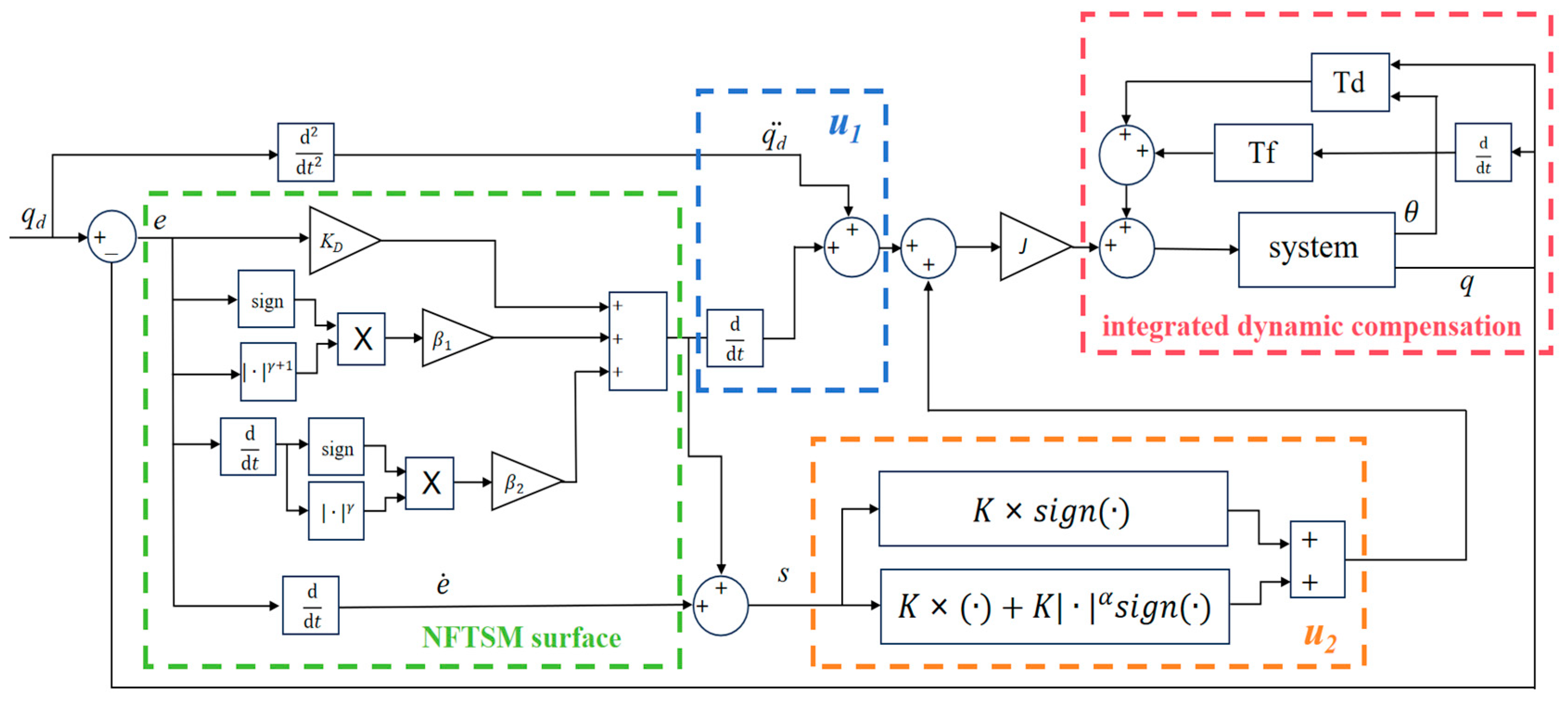
3. Controller Design and Stability Analysis

3.1. Control Design

As shown in Figure 3, we propose an enhanced sliding variable and reaching law of the non-singular fast terminal sliding mode. First, the NFTSM surface and reaching law are designed as follows:

$$s=\dot{e}+K_{D}e+{\beta }_1{|e|}^{\gamma +1}sign(e)+{\beta }_2{|\dot{e}|}^{\gamma }sign(\dot{e}),$$

(8)

where $e$ represents the tracking error and its time derivative is given as follows:

$$\dot{s}=\ddot{e}+K_D\dot{e}+{\beta }_1(\gamma +1){|e|}^{\gamma }\dot{e}+{\beta }_2\gamma {|\dot{e}|}^{\gamma -1}\ddot{e},$$

(9)

$$e=q_d-q,$$

(10)

where $q_d$ represents the ideal angular displacement, $K_D>0$, ${\beta }_1>0$, ${\beta }_2>0$ and $1<\gamma <$ 2.

The control law is designed as follows:

$$u_1=J\left({\ddot{q}}_d+K_D\dot{e}+{\beta }_1\left(\gamma +1\right){\left|e\right|}^{\gamma }\dot{e}+{\beta }_2\gamma {\left|\dot{e}\right|}^{\gamma -1}\ddot{e}\right),$$

(11)

$$u_2=J(Ks+K\times sign(s)+K{|s|}^{\alpha }sign(s)),$$

(12)

$$T_M=u_1+u_2+\widehat{T},$$

(13)

where $0<\alpha <1$.

The adaptive gain $K$ is designed as follows:

$$\dot{K}=\left\{\begin{array}{l}\lambda {|s|}^{sign(|s|-\delta K^2)}sign(|s|-\delta K^2),K>0\\ \lambda |s|,K=0\end{array}\right.,$$

(14)

where $\lambda >$ 0 and $\delta >0$.

For $K>0$, the adaptive law has two different forms: $|s|>\delta K^2$ and $|s|<\delta K^2$. When $|s|>\delta K^2$, the switching gain $K$ increases until $|s|<\delta K^2$. As the switching gain $\mathrm{K}$ becomes larger, the sliding variable $s$ reaches the vicinity of the sliding manifold faster. When $|s|<\delta K^2$, the switching gain $K$ decreases.

3.2. Stability Analysis

Theorem 1.

For an n-degree-of-freedom robot manipulator system, under the NFTSM surface and control law, a Lyapunov function is constructed and it is proven that its derivative is semi-negative definite, and the dynamic system corresponding to the algorithm is stable.

Proof. 

To demonstrate the stability of the proposed method (8), a Lyapunov-like function is defined as follows:

$$V={\displaystyle \frac{1}{2}}{s}^{{\rm T}}s+{\displaystyle \frac{1}{2}}{\sum }_{i=1}^n{\displaystyle \frac{1}{{\lambda }_i}}{(K_i-{J_i}^{-1}{{\mathit{\Delta }}_i}^{*})}^2,$$

(15)

where ${{\mathit{\Delta }}_i}^{*}$ is a constant, which is defined as follows:

$${{\mathit{\Delta }}_i}^{*}\ge {||{\mathit{\Delta }}_i||}_{\infty }={||T_i-{\widehat{T}}_i||}_{\infty }.$$

(16)

Based on (15), its time derivative is given as:

$$\dot{V}={\sum }_{i=1}^n{(s_i}^2+{\displaystyle \frac{1}{{\lambda }_i}}(K_i-{J_i}^{-1}{{\mathit{\Delta }}_i}^{*})\dot{\times K_i)}.$$

(17)

Substitute Equation (9) and ${\ddot{e}}_i={\ddot{q}}_{d,i}-{\ddot{q}}_i$ into (17):

$$\dot{V}={\sum }_{i=1}^n{s}_i({\ddot{q}}_{d,i}-{\ddot{q}}_i+K_D\dot{e_i}+{\beta }_{1i}{(\gamma }_i+1){|e_i|}^{{\gamma }_i}{\dot{e}}_i+{\beta }_{2i}{\gamma }_i{|{\dot{e}}_i|}^{{\gamma }_i-1}{\ddot{e}}_i)+{\sum }_{i=1}^n{\displaystyle \frac{1}{{\lambda }_i}}(K_i-{J_i}^{-1}{{\mathit{\Delta }}_i}^{*})\dot{K_i}.$$

(18)

Substitute Equations (2) and (13) into (18):

$$\dot{V}={\sum }_{i=1}^n{s}_i({\ddot{q}}_{d,i}-{J_i}^{-1}\left(T_{m,i}-T_{\mathrm{f},i}-T_{\mathrm{d},i}\right)+K_D\dot{e_i}+{\beta }_{1i}{(\gamma }_i+1){\left|e_i\right|}^{{\gamma }_i}{\dot{e}}_i+{\beta }_{2i}{\gamma }_i{\left|{\dot{e}}_i\right|}^{{\gamma }_i-1}{\ddot{e}}_i)+{\sum }_{i=1}^n{\displaystyle \frac{1}{{\lambda }_i}}(K_i-{J_i}^{-1}{{\mathit{\Delta }}_i}^{*})\dot{K_i}.$$

(19)

Substitute Equations (11)–(13) into (19):

$$\begin{array}{cc}& \dot{V}={\sum }_{i=1}^n{s}_i({\ddot{q}}_{d,i}-{J_i}^{-1}(J_i({\dot{q}}_{d,i}+K_D\dot{e_i}+{\beta }_{1i}{(\gamma }_i+1){|e_i|}^{{\gamma }_i}{\dot{e}}_i+{\beta }_{2i}{\gamma }_i{|{\dot{e}}_i|}^{{\gamma }_i-1}{\ddot{e}}_i+K_i{s}_i+K_{i}sign(s_i)+\\ & K_i{|s_i|}^{{\alpha }_i}sign(s_i))+{\widehat{T}}_i-T_i)+K_D\dot{e_i}+{\beta }_{1i}{(\gamma }_i+1){|e_i|}^{{\gamma }_i}{\dot{e}}_i+{\beta }_{2i}{\gamma }_i{|{\dot{e}}_i|}^{{\gamma }_i-1}{\ddot{e}}_i)+{\sum }_{i=1}^n{\displaystyle \frac{1}{{\lambda }_i}}(K_i-{J_i}^{-1}{{\mathit{\Delta }}_i}^{*})\dot{K_i}.\end{array}$$

(20)

Simplifying (20), we obtain the following by substituting (16):

$$\begin{array}{cc}& \dot{V}={\sum }_{i=1}^n{s}_i(-K_i{s}_i{{-K_{i}sign(s_i)-K_i{|s_i|}^{{\alpha }_i}sign(s_i)+J}_i}^{-1}{\mathit{\Delta }}_i)+{\sum }_{i=1}^n{\displaystyle \frac{1}{{\lambda }_i}}(K_i-{J_i}^{-1}{{\mathit{\Delta }}_i}^{*})\dot{K_i}=\\ & {\sum }_{i=1}^n(-K_i{s_i}^2)+{\sum }_{i=1}^n(-K_i{|s}_i|)+{\sum }_{i=1}^n{(-K}_i{|s_i|}^{{\alpha }_i+1})+{\sum }_{i=1}^n{J_i}^{-1}{\mathit{\Delta }}_i|s_i|+{\sum }_{i=1}^n{\displaystyle \frac{1}{{\lambda }_i}}(K_i-{J_i}^{-1}{{\mathit{\Delta }}_i}^{*})\dot{K_i}.\end{array}$$

(21)

When $K>0$

$$\begin{array}{cc}& \dot{V}={\sum }_{i=1}^n(-K_i{s_i}^2)+{\sum }_{i=1}^n(-K_i{|s}_i|)+{\sum }_{i=1}^n{(-K}_i{|s_i|}^{{\alpha }_i+1})+{\sum }_{i=1}^n{J_i}^{-1}{\mathit{\Delta }}_i|s_i|+{\sum }_{i=1}^n{\displaystyle \frac{1}{{\lambda }_i}}(K_i-\\ & {J_i}^{-1}{{\mathit{\Delta }}_i}^{*})\lambda {|s|}^{sign(|s|-\delta K^2)}sign(|s|-\delta K^2).\end{array}$$

(22)

In Equation (23), when $|s_i|>\delta K^2$:

$$\begin{array}{cc}& \dot{V}={\sum }_{i=1}^n(-K_i{s_i}^2-K_i{|s}_i|{-K}_i{|s_i|}^{{\alpha }_i+1}+{J_i}^{-1}{\mathit{\Delta }}_i|s_i|+K_i|s_i|-{J_i}^{-1}{{\mathit{\Delta }}_i}^{*}|s_i|)\le {\sum }_{i=1}^n(-K_i{s_i}^2-\\ & K_i{|s}_i|{-K}_i{|s_i|}^{{\alpha }_i+1}+K_i|s_i|)={\sum }_{i=1}^n(-K_i{s_i}^2{{-K}_i|s_i|}^{{\alpha }_i+1}).\end{array}$$

(23)

Therefore, when $K>0\mathrm{a}\mathrm{n}\mathrm{d}|s_i|>\delta K^2$, $\dot{V}\le$ 0.

When $0<|s_i|\le \delta K^2$, $K$ must satisfy the following conditions:

$$\begin{array}{cc}& \dot{V}={\sum }_{i=1}^n(-K_i{s_i}^2-K_i{|s}_i|{-K}_i{|s_i|}^{{\alpha }_i+1}+{{J_i}^{-1}\mathit{\Delta }}_i|s_i|{-K_i|s_i|}^{-1}+{J_i}^{-1}{{\mathit{\Delta }}_i}^{*}{|s_i|}^{-1})\le {\sum }_{i=1}^n(-K_i{s_i}^2-\\ & K_i{|s}_i|{-K}_i{|s_i|}^{{\alpha }_i+1}+{J_i}^{-1}{{\mathit{\Delta }}_i}^{*}|s_i|-K_i{|s_i|}^{-1}+{J_i}^{-1}{{\mathit{\Delta }}_i}^{*}{|s_i|}^{-1}).\end{array}$$

(24)

In order to make $\dot{V}\le$ 0, $K$ must satisfy the following conditions:

$$K_i\ge {\displaystyle \frac{{J_i}^{-1}{{\mathit{\Delta }}_i}^{*}(|s_i|+{|s_i|}^{-1})}{{s_i}^2+|s_i|+{|s_i|}^{{\alpha }_i+1}+{|s_i|}^{-1}}}.$$

(25)

When $K=0$, $\dot{K}=\lambda |s|$:

$$\dot{V}={\sum }_{i=1}^n(-K_i{s_i}^2)+{\sum }_{i=1}^n(-K_i{|s}_i|)+{\sum }_{i=1}^n{(-K}_i{|s_i|}^{{\alpha }_i+1})+{\sum }_{i=1}^n{J_i}^{-1}{\mathit{\Delta }}_i|s_i|+{\sum }_{i=1}^n{\displaystyle \frac{1}{{\lambda }_i}}(K_i-{J_i}^{-1}{{\mathit{\Delta }}_i}^{*})\lambda |s|\le 0.$$

(26)

□

4. Experiments

4.1. Experimental Setup

To demonstrate the performance of the proposed scheme, the experiment employs a robot manipulator torque joint motor integrated performance development platform, as shown in Figure 4. The platform consists of a robot manipulator joint module, a torque sensor, an eddy current brake, a control system, and computer-based host software. The drive motor of the robot manipulator joint module has a rated voltage of 48 (V), a rated current of 2.7 (A), and a rated speed of 5000 (rpm). The motor’s moment of inertia is $J$ = 0.244 × 10⁻⁴ (kg·m²), and the gear ratio is N = 100.

In this set of experiments, the control algorithm proposed in this paper was modeled in a modular form using MATLAB 2020b and Simulink simulation software. After compilation, it was converted into the C language, which can be executed by the CSPACE controller to generate control signals. These signals are then sent to the motor driver to achieve real-time control of the motor.

To verify the tracking performance of the proposed control algorithm, comparative experiments were conducted with three control schemes: PID, NFTSM, and NFTSM combined with T_f. The three control schemes are as follows:

$$T_{PID}=K_{p}e+K_i\int edt+K_d\dot{e},$$

(27)

$$T_{NFTSM}=u_1+u_2,$$

(28)

$$T_{NFTSM+T\mathrm{f}}=u_1+u_2+{\widehat{T}}_{\mathrm{f}},$$

(29)

The desired trajectory for all the experiments was designed as $q_d$ = 30sin(πt/4), with a sampling time of 0.05(s). The PID control parameters were set as $K_p$ = 9500, $K_i$ = 1, $K_d$ = 80. The parameters for the NFTSM control algorithm were set as $K_D$ = 60, ${\beta }_1$ = 15, $\gamma$ = 1.3, ${\beta }_2$ = 1.2, $\lambda$ = 0.5, $\alpha$ = 0.4 and $\delta$ = 1.3.

The experiments were designed as follows:

• Experiment 1: Trajectory tracking experiments using the four control schemes mentioned above under zero load conditions.
• Experiment 2: Trajectory tracking experiments using the four control schemes under a 5 (N) constant load.
• Experiment 3: Trajectory tracking experiments using the four control schemes under a sinusoidal load.
• Experiment 4: Trajectory tracking experiments using the four control schemes under a step load.

In the experimental results, the control performance of the algorithms was quantitatively evaluated using two metrics: root mean square error and maximum error. The specific definitions are as follows:

$$\mathrm{RMSE}=\sqrt{{\displaystyle \frac{{\sum }_{\mathrm{i}=1}^{\mathrm{N}}{e}_i^2}{\mathrm{N}}}},$$

(30)

$$\mathrm{MAXE}=\mathrm{m}\mathrm{a}\mathrm{x}(|e_i|),$$

(31)

where N represents the number of samples.

4.2. Experimental Results

• Experiment 1: For all the control schemes, no load was applied. The actual position and tracking errors are shown in Figure 5a,b. Compared with the PID control scheme, the NFTSM scheme can significantly reduce the tracking error. The introduction of friction compensation further reduces the tracking error compared to using the NFTSM scheme alone. Under no-load conditions, friction exerts noticeable interference on the robot manipulators’ trajectory tracking. Adding friction compensation can reduce the tracking error. The motor input torque is shown in Figure 5c. When the system is not disturbed by external loads, the error mainly originates from internal factors of the system. The external torque estimation compensation has a negligible impact on the system dynamics. To simplify the control strategy, unnecessary compensation components are reduced under no-load conditions to lower the complexity and computational burden. As shown in Figure 5d, the dynamic changes in the adaptive factor indicate that when the system tracking error is large, the adaptive factor increases to enhance the control effect, thereby further reducing the error and improving the tracking accuracy. Conversely, when the system stabilizes or the control input is too large, the adaptive factor decreases to control the magnitude of the input, avoiding over-control or energy waste. As shown in

  Table 3. RMSE and MAXE for trajectory tracking under no-load conditions.

  Control Schemes	RMSE (Deg)	MAXE (Deg)
  PID	0.11380	0.20000
  NFTSM	0.07194	0.11000
  NFTSM+Tf	0.02923	0.07000

  , the experimental results of each algorithm in terms of the RMSE and MAXE for trajectory tracking under no-load conditions are presented. Comparisons reveal that the control algorithm proposed in this paper has smaller values for both the RMSE and MAXE compared to the other three control schemes. Therefore, the proposed algorithm can more accurately match the target trajectory, achieving a higher level of trajectory tracking performance.

2.

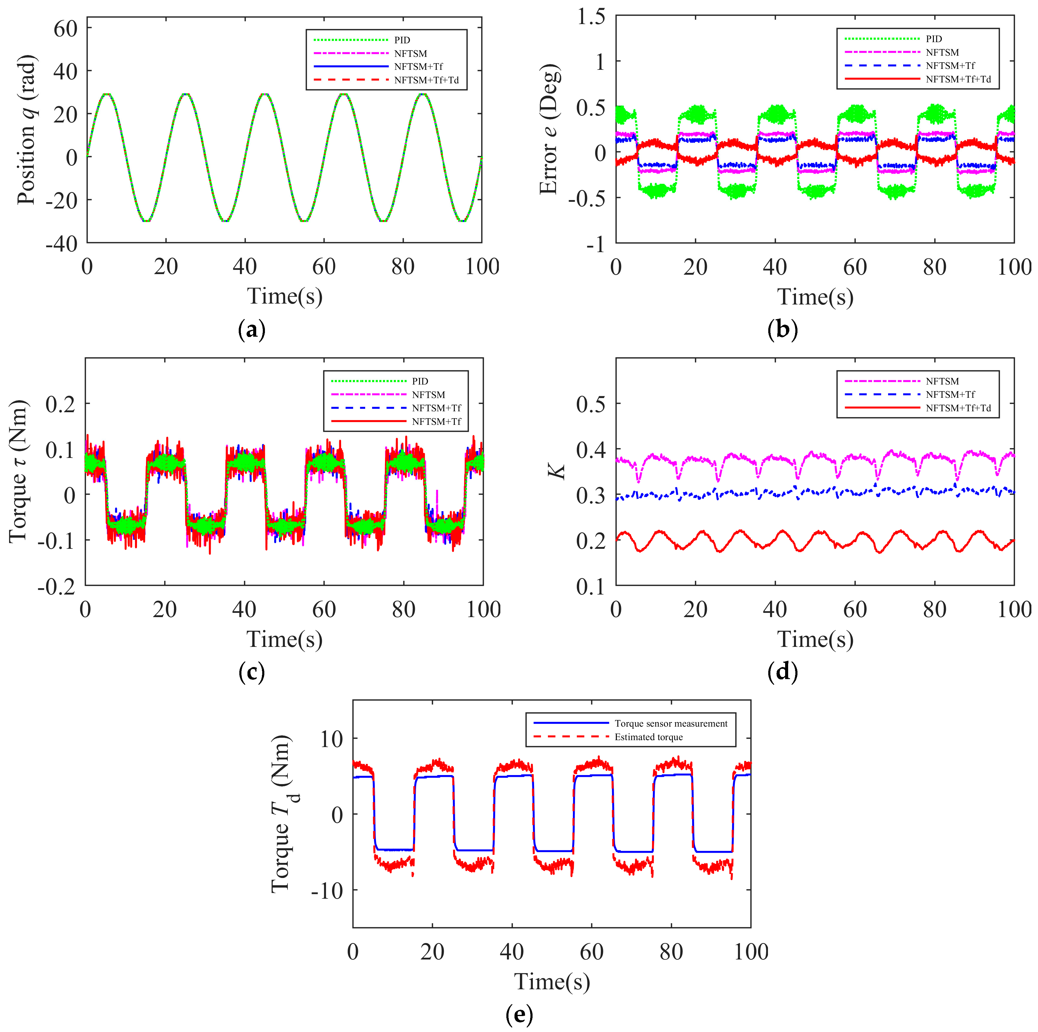
Experiment 2: A constant load (5 Nm) was applied to all the control schemes. The actual position and tracking errors are shown in Figure 6a,b. The experimental results demonstrate that, under a constant load, the NFTSM scheme can significantly reduce the tracking error compared with PID control. Under a constant load, the impact of friction interference on the system is relatively small, and the addition of friction compensation has little effect on improving the control accuracy. However, when the NFTSM scheme is combined with both friction compensation and joint torque compensation, the root mean square error and maximum error values are further reduced, achieving even smaller tracking errors. As shown in Figure 6c, the motor input torque increases after adding friction compensation and joint torque compensation. As shown in Figure 6d, the adaptive factor K decreases after adding friction compensation and joint torque compensation. As shown in Figure 6e, the estimated torque is close to the load torque, which justifies the joint torque compensation in the scheme. The RMSE and MAXE values for trajectory tracking under the condition of a constant load for each control algorithm are shown in

Table 4. RMSE and MAXE for trajectory tracking under constant load conditions.

Control Schemes	RMSE (Deg)	MAXE (Deg)
PID	0.40422	0.53000
NFTSM	0.19836	0.24000
NFTSM+Tf	0.14700	0.20000
NFTSM+Tf+Td	0.08138	0.18000

. Therefore, the proposed control algorithm can still maintain a higher level of trajectory tracking accuracy under constant load conditions.

3.

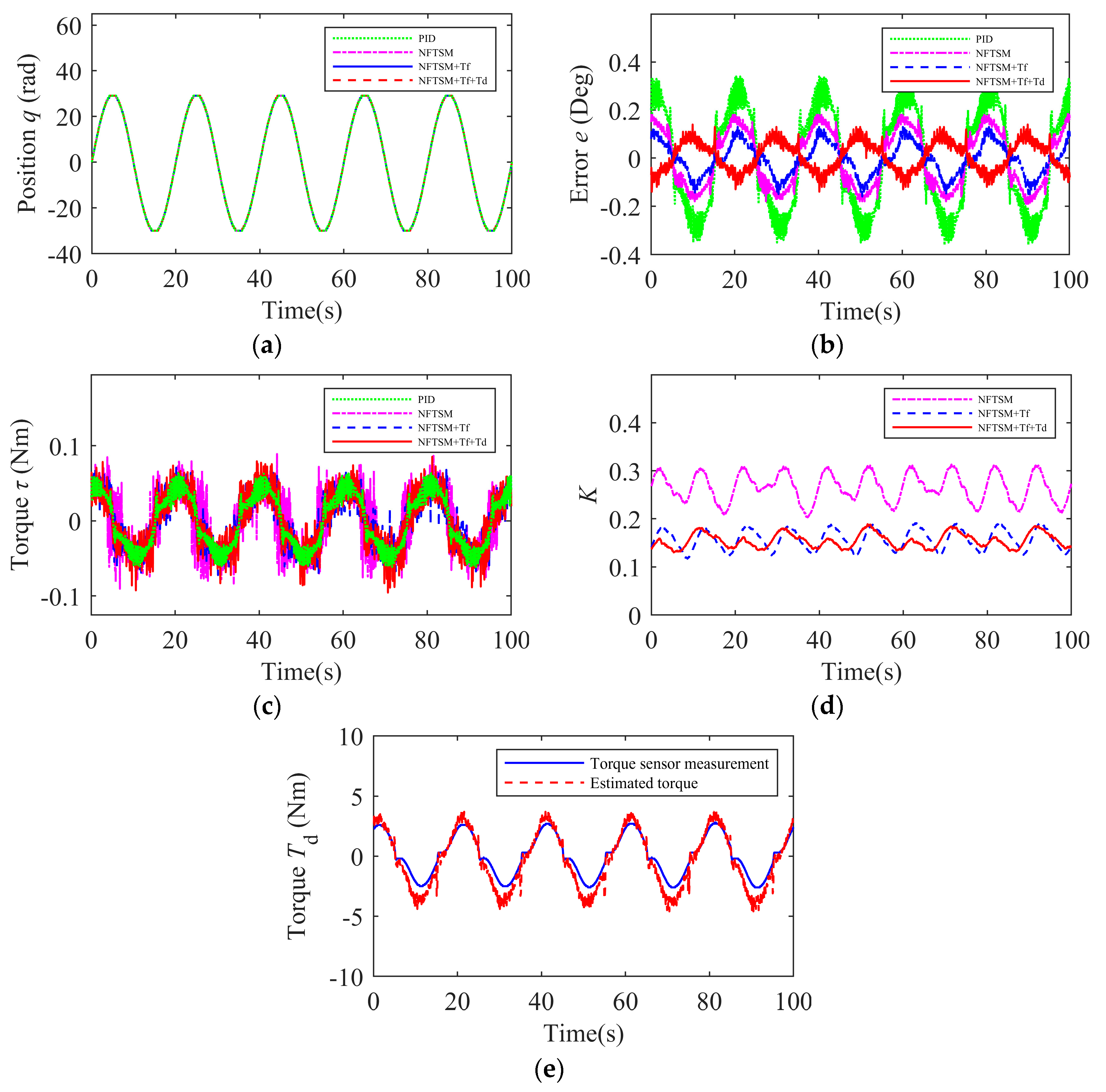
Experiment 3: A sinusoidal load was applied to all the control schemes. The actual position and tracking errors are shown in Figure 7a,b. Figure 7c displays the motor input torque, Figure 7d shows the variation of the adaptive gain, and Figure 7e presents the estimation results of the load torque. The root mean square error and maximum error values for trajectory tracking under sinusoidal load conditions for each control algorithm are shown in

Table 5. RMSE and MAXE for trajectory tracking under sinusoidal load conditions.

Control Schemes	RMSE (Deg)	MAXE (Deg)
PID	0.21029	0.36000
NFTSM	0.11978	0.19000
NFTSM+Tf	0.06694	0.16000
NFTSM+Tf+Td	0.05867	0.14000

. The experimental results indicate that, compared with the other three control schemes, the proposed control algorithm has smaller RMSE and MAXE values in terms of the tracking error. Therefore, it can be concluded that the proposed control algorithm can still maintain a higher level of trajectory tracking accuracy and rapid adaptability under sinusoidal load conditions.

4.

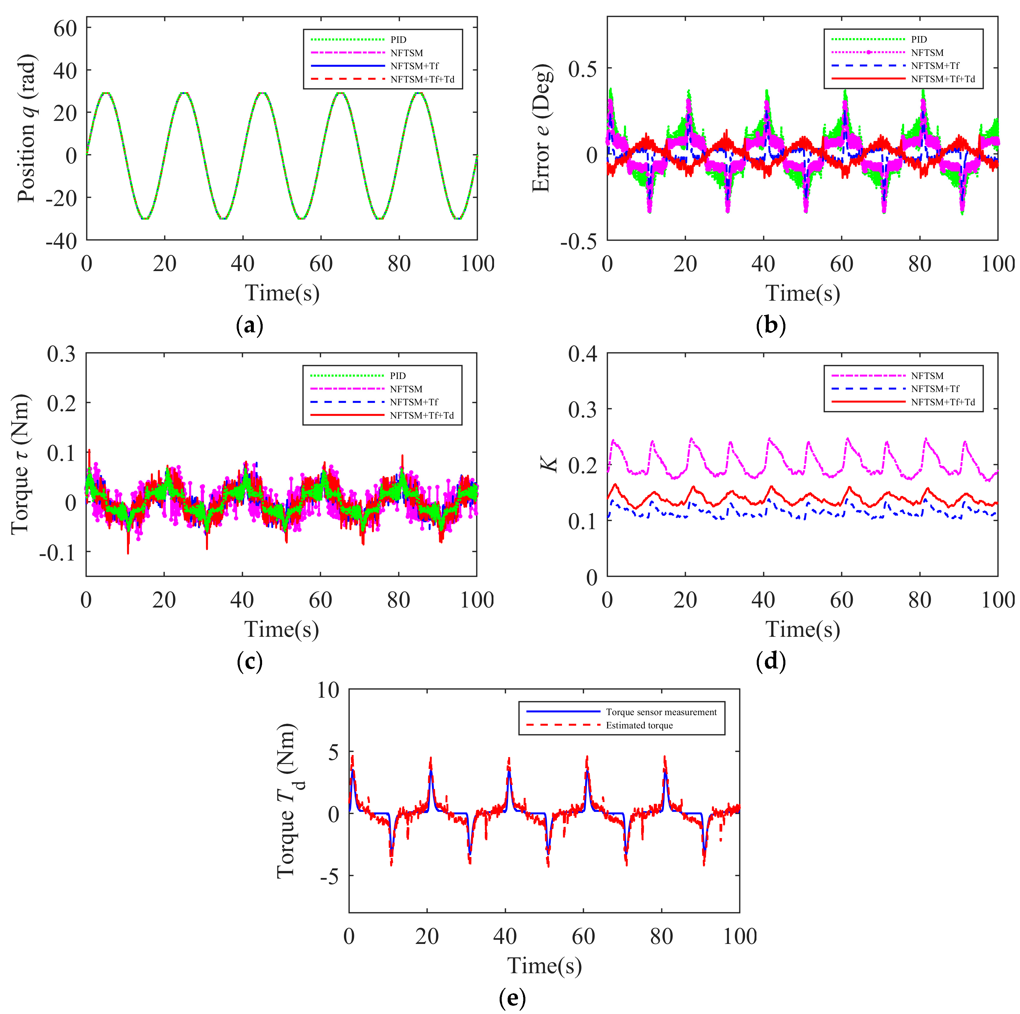
Experiment 4: A step load was applied to all the control schemes. The actual position and tracking errors are shown in Figure 8a,b. Figure 8c displays the motor input torque, Figure 8d shows the variation of the adaptive gain, and Figure 8e presents the estimation results of the load torque. The root mean square error and maximum error values for trajectory tracking under step load conditions for each control algorithm are shown in

Table 6. RMSE and MAXE for trajectory tracking under step load conditions.

Control Schemes	RMSE (Deg)	MAXE (Deg)
PID	0.14108	0.38000
NFTSM	0.10290	0.33000
NFTSM+Tf	0.05796	0.27000
NFTSM+Tf+Td	0.05213	0.14000

. The experimental results indicate that, compared with the other three control schemes, the proposed control algorithm has smaller RMSE and MAXE values in terms of the tracking error. Therefore, it can be concluded that the proposed control algorithm can still maintain a higher level of trajectory tracking accuracy and rapid adaptability under step load conditions.

5. Conclusions

This paper presents a non-singular fast terminal sliding mode tracking controller for robot manipulators and develops an integrated dynamic compensation control strategy involving friction compensation and joint torque compensation to improve the trajectory tracking accuracy of robot manipulators under variable load conditions. The friction compensation takes into account friction factors related to the velocity, while the joint torque compensation considers the torsional errors and motion errors of the flexible robot manipulators, thereby enhancing the compensation accuracy. The stability of the controller is guaranteed by Lyapunov’s theory. Comparative experiments were conducted using a robot manipulator torque joint motor integrated platform. The proposed control scheme demonstrated smaller root mean square error (RMSE) and maximum error (MAXE) values in terms of trajectory tracking, thereby validating the effectiveness of the control strategy.

References

- Li, Y.; Ang, K.H.; Chong, G.C. PID Control System Analysis and Design. IEEE Control Syst. Mag. 2006, 26, 32–41. [Google Scholar] [CrossRef]
- Zhao, Y.; Qi, J.; Li, W. Adaptive PID Feedback Tracking Control for 6-DOF Collaborative Robot. In Proceedings of the 2022 34th Chinese Control and Decision Conference (CCDC), Hefei, China, 15–17 August 2022; pp. 5525–5532. [Google Scholar] [CrossRef]
- Zhang, L.; Su, Y.; Wang, Z.; Wang, H. Fixed-Time Terminal Sliding Mode Control for Uncertain Robot Manipulators. ISA Trans. 2024, 144, 364–373. [Google Scholar] [CrossRef] [PubMed]
- Zhu, Y.; Qiao, J.; Guo, L. Adaptive Sliding Mode Disturbance Observer-Based Composite Control with Prescribed Performance of Space Manipulators for Target Capturing. IEEE Trans. Ind. Electron. 2019, 66, 1973–1983. [Google Scholar] [CrossRef]
- Spong, M.W.; Ortega, R.; Kelly, R. Comments on “Adaptive Manipulator Control: A Case Study” by J. Slotine and W. Li. IEEE Trans. Autom. Control 1990, 35, 761–762. [Google Scholar] [CrossRef]
- Wang, H.; Xu, K.; Zhang, H. Adaptive Finite-Time Tracking Control of Nonlinear Systems With Dynamics Uncertainties. IEEE Trans. Autom. Control 2023, 68, 5737–5744. [Google Scholar] [CrossRef]
- Bouakrif, F.; Zasadzinski, M. Trajectory Tracking Control for Perturbed Robot Manipulators Using Iterative Learning Method. Int. J. Adv. Manuf. Technol. 2016, 87, 2013–2022. [Google Scholar] [CrossRef]
- Kou, Z.; Sun, J. Test-Based Model-Free Adaptive Iterative Learning Control with Strong Robustness. Int. J. Syst. Sci. 2023, 54, 1213–1228. [Google Scholar] [CrossRef]
- Chaoui, H.; Gueaieb, W. Type-2 Fuzzy Logic Control of a Flexible-Joint Manipulator. J. Intell. Robot. Syst. 2008, 51, 159–186. [Google Scholar] [CrossRef]
- Van, M.; Sun, Y.; Mcllvanna, S.; Nguyen, M.-N.; Khyam, M.O.; Ceglarek, D. Adaptive Fuzzy Fault Tolerant Control for Robot Manipulators With Fixed-Time Convergence. IEEE Trans. Fuzzy Syst. 2023, 31, 3210–3219. [Google Scholar] [CrossRef]
- Peng, R.; Guo, R.; Zheng, B.; Miao, Z.; Zhou, J. Neural Network-Based Robust Consensus Tracking for Uncertain Networked Euler-Lagrange Systems with Time-Varying Delays and Output Constraints. Appl. Math. Comput. 2024, 468, 128522. [Google Scholar] [CrossRef]
- Zhu, C.; Jiang, Y.; Yang, C. Fixed-Time Neural Control of Robot Manipulator With Global Stability and Guaranteed Transient Performance. IEEE Trans. Ind. Electron. 2023, 70, 803–812. [Google Scholar] [CrossRef]
- Shi, D.; Zhang, J.; Sun, Z.; Xia, Y. Adaptive Sliding Mode Disturbance Observer-Based Composite Trajectory Tracking Control for Robot Manipulator with Prescribed Performance. Nonlinear Dyn. 2022, 109, 2693–2704. [Google Scholar] [CrossRef]
- Yu, S.; Yu, X.; Shirinzadeh, B.; Man, Z. Continuous Finite-Time Control for Robotic Manipulators with Terminal Sliding Mode. Automatica 2005, 41, 1957–1964. [Google Scholar] [CrossRef]
- Feng, Y.; Yu, X.; Man, Z. Non-Singular Terminal Sliding Mode Control of Rigid Manipulators. Automatica 2002, 38, 2159–2167. [Google Scholar] [CrossRef]
- Yin, S.; Shi, Z.; Liu, Y.; Xue, G.; You, H. Adaptive Non-Singular Terminal Sliding Mode Trajectory Tracking Control of Robotic Manipulators Based on Disturbance Observer Under Unknown Time-Varying Disturbance. Processes 2025, 13, 266. [Google Scholar] [CrossRef]
- Zhang, Y.; Fang, L.; Song, T.; Zhang, M. Adaptive Non-singular Fast Terminal Sliding Mode Based on Prescribed Performance for Robot Manipulators. Asian J. Control 2023, 25, 3253–3268. [Google Scholar] [CrossRef]
- Jiang, J.; Zhang, H.; Jin, D.; Wang, A.; Liu, L. Disturbance Observer Based Non-Singular Fast Terminal Sliding Mode Control of Permanent Magnet Synchronous Motors. J. Power Electron. 2024, 24, 249–257. [Google Scholar] [CrossRef]
- Zhuang, X.; Guo, Y.; Tian, Y.; Wang, H. A Sampled Delayed Output Extended State Observer-Based Adaptive Feedback Control of Robot Manipulator with Unknown Dynamics. Nonlinear Dyn. 2023, 111, 22283–22301. [Google Scholar] [CrossRef]
- Saleki, A.; Fateh, M.M. Model-Free Control of Electrically Driven Robot Manipulators Using an Extended State Observer. Comput. Electr. Eng. 2020, 87, 106768. [Google Scholar] [CrossRef]
- Zhang, Z.; Hu, X.; Huang, P. Disturbance Observer-Based Tracking Controller for n-Link Flexible-Joint Robots Subject to Time-Varying State Constraints. Electronics 2024, 13, 1773. [Google Scholar] [CrossRef]
- Zhang, D.; Hu, J.; Cheng, J.; Wu, Z.-G.; Yan, H. A Novel Disturbance Observer Based Fixed-Time Sliding Mode Control for Robotic Manipulators with Global Fast Convergence. IEEECAA J. Autom. Sin. 2024, 11, 661–672. [Google Scholar] [CrossRef]
- Lee, J.; Chang, P.H.; Jin, M. Adaptive Integral Sliding Mode Control with Time-Delay Estimation for Robot Manipulators. IEEE Trans. Ind. Electron. 2017, 64, 6796–6804. [Google Scholar] [CrossRef]
- Taefi, M.; Khosravi, M.A. A Model Free Adaptive-robust Design for Control of Robot Manipulators: Time Delay Estimation Approach. Int. J. Robust Nonlinear Control 2024, 34, 8227–8247. [Google Scholar] [CrossRef]
- Wang, G.; Wang, Z.; Huang, B.; Gan, Y.; Min, F. Active Compliance Control Based on EKF Torque Fusion for Robot Manipulators. IEEE Robot. Autom. Lett. 2023, 8, 2668–2675. [Google Scholar] [CrossRef]
- Bona, B.; Indri, M. Friction Compensation in Robotics: An Overview. In Proceedings of the 44th IEEE Conference on Decision and Control, Seville, Spain, 15 December 2005; pp. 4360–4367. [Google Scholar] [CrossRef]
- Liang, X.; Yao, Z.; Deng, W.; Yao, J. Adaptive Control of N-Link Hydraulic Manipulators with Gravity and Friction Identification. Nonlinear Dyn. 2023, 111, 19093–19109. [Google Scholar] [CrossRef]
- Thenozhi, S.; Sanchez, A.C.; Rodriguez-Resendiz, J. A Contraction Theory-Based Tracking Control Design with Friction Identification and Compensation. IEEE Trans. Ind. Electron. 2022, 69, 6111–6120. [Google Scholar] [CrossRef]
- Ghorbel, F.H.; Gandhi, P.S.; Alpeter, F. On the Kinematic Error in Harmonic Drive Gears. J. Mech. Des. 1998, 123, 90–97. [Google Scholar] [CrossRef]
- Song, Y.; Huang, H.; Liu, F.; Xi, F.; Zhou, D.; Li, B. Torque Estimation for Robotic Joint with Harmonic Reducer Based on Deformation Calibration. IEEE Sens. J. 2020, 20, 991–1002. [Google Scholar] [CrossRef]