Article

Disturbance Rejection Approach for Nonlinear Systems Using Kalman-Filter-Based Equivalent-Input-Disturbance Estimator

1
School of Information Science and Technology, Beijing University of Technology, Beijing 100124, China
2
Xi’an Modern Control Technology Research Institute, Xi’an 710065, China
*
Author to whom correspondence should be addressed.
Actuators 2025, 14(4), 189; https://doi.org/10.3390/act14040189
Submission received: 11 March 2025 / Revised: 6 April 2025 / Accepted: 10 April 2025 / Published: 11 April 2025
(This article belongs to the Section Control Systems)

Abstract

:
In this paper, a novel disturbance rejection approach is developed for a class of nonlinear systems, which incorporates the Kalman filter into the equivalent-input-disturbance (EID) structure. First, the EID-based control system and the configuration of the Kalman Filter are illustrated. Then, an optimal estimation theorem is obtained by analyzing the dynamic of the Kalman filter, and a special Kalman gain is derived. Next, the dynamics of the closed-loop system are deduced, and stability is guaranteed based on the Lyapunov function. Finally, simulations with comparison are carried out to demonstrate the excellent performance of both disturbance rejection and noise attenuation.

1. Introduction

Disturbances are ubiquitous in industrial systems, arising from factors such as sensor noise [1], load variations, and external disturbances [2]. These disturbances will degrade the control performance and even lead to system instability. Consequently, disturbance rejection continues to be a fundamental challenge in control engineering, particularly for nonlinear systems [3,4,5]. On the other hand, due to the inevitable noise, it is crucial to consider the noise effect in the controller design process. This limitation highlights the necessity for novel control methods that integrate disturbance estimation, state observation, and noise attenuation into a comprehensive framework.
To effectively reject disturbances, there are some active disturbance rejection (ADR) methods, such as the Extended State Observer (ESO), the Disturbance Observer (DOB), and the Equivalent-Input-Disturbance (EID) method. The ESO method treats the lumped disturbance (including system uncertainties, external disturbances, and nonlinearities) as an extended state [6], but the states require availability in controller design. The DOB method uses the inverse of a nominal plant to estimate and reduce the effect of disturbances [7], which may not be realizable in practice. The EID method, as an active disturbance rejection method, has been widely used in physical systems due to its simple structure [8,9,10,11]. It applies an artificial disturbance to the control input, which produces an equivalent effect to the real disturbance on the system output [12]. Recently, a convenient version of the EID method (CEID) has been developed, which uses a linear gain in the CEID-based estimator to tune the disturbance rejection performance [13]. However, a large estimator gain may lead to increased sensitivity to noise, which burdens the actuators and even unstabilizes the whole control system.
As a cornerstone of optimal state estimation, the Kalman filter provides a robust framework for state estimation under noise in dynamic systems [14,15,16]. For systems with partially known nonlinear mapping, conventional Kalman filters usually handle nonlinearities through linearization [17] or sigma-point transformations [18,19]. However, these approaches use the complex error covariance update policy to calculate the Kalman gain online, resulting in high computational costs and poor real-time performance. Recently, a steady-state Kalman filter was developed to address disturbance and noise with an ESO, which shows advantages in noise attenuation and other control performance [20]. In particular, its steady-state Kalman gain shows excellent advantages in computational efficiency instead of a time-varying one, making it ideal for real-time applications.
Enlightened by the above discussion, this paper proposed a novel Kalman-Filter-based Equivalent-Input-Disturbance-based Estimator (KF-EIDE) for a class of nonlinear systems with disturbances and measurement noise. The primary objective of this study is to bridge the gap between disturbance rejection and noise attenuation in nonlinear control systems by integrating CEID and steady-state Kalman filter, while explicitly incorporating prior knowledge of system nonlinearities.
Unlike existing methods, key contributions are made:
  • Novelty in methodology: a novel KF-EIDE scheme is organically proposed, which combines the disturbance rejection capability of CEID with the noise attenuation capability of the Kalman filter to improve the system tracking performance.
  • Improvement of structure: nonlinear dynamics and the Kalman filter are organically integrated with the CEID control scheme, enabling accurate state estimation.
  • Theoretical rigor: under the lumped disturbance, nonlinearity, and measurement noise, the stability of the closed-loop control system is guaranteed.
The rest of this paper is organized as follows: Section 2 demonstrates the problem and presents the nonlinear system model with disturbance dynamics. Section 3 details the design of the KF-EIDE and gives the related theorem, including nonlinearity incorporation mechanisms. Section 4 analyzes and proves the stability of the whole closed-loop control system. Section 5 validates the method through comparative simulations on a classic nonlinear system, while Section 6 gives the conclusion with future research directions.
In this paper, some mathematical symbols are first denoted as follows: R q × p presents the set of real matrices with q rows and p columns; W ( s ) stands for the Laplace transform of a continuous-time signal w ( t ) ; I denotes the identity matrix of appropriate dimensions; diag { · } refers to the diagonal matrix; | a | and A are the absolute value of a scalar a and the 2-norm of a matrix A, respectively; α ( t ) is the 2-norm of a vector α ( t ) ; and the time t will be excluded if the context provides clarity.

2. Methods and Materials

2.1. Problem Formulation

Consider a class of single-input single-output (SISO) nonlinear systems with measurement noise:
x ˙ ( t ) = A x ( t ) + f ( x ( t ) ) + B u ( t ) + B d d ( t ) y o ( t ) = C x ( t ) y ( t ) = C x ( t ) + v ( t )
where x ( t ) R n is the system state; u ( t ) R , y o ( t ) R , and y ( t ) R are the control input, control output, and measurement output, respectively; f ( · ) : R n R n is a known nonlinear mapping; v ( t ) is the measurement noise that is usually caused by sensors; d ( t ) R d is a lumped disturbance term incorporating both system parameter perturbation and environmental disturbances; B d R n × n d is the unknown disturbance input matrix subject to d ( t ) ; and A, B, and C are is the system parameter matrices with appropriate dimensions.
For the system in (1), some assumptions are made as follows.
Assumption  1.
The controllability of the pair ( A , B ) and the observability of the pair ( A , C ) hold.
Assumption  2.
The unknown lumped disturbance d ( t ) of the system has an upper bound, i.e.,
d ( t ) d m
where d m is an unknown positive constant.
Assumption  3.
The nonlinear mapping f ( · ) is obtained by some techniques and satisfies
f ( x 1 ) f ( x 2 ) f m x 1 x 2 f ( 0 ) = f 0
where x 1 , x 2 R n ; f m is a known positive constant number; and f 0 is a known constant.
Remark  1.
Assumption 1 usually holds in controller design, and the boundedness constraints in Assumption 2 are universally valid in engineering practice.
Remark  2.
The prior knowledge of f ( · ) can usually be known through system identification or other techniques. On the other hand, the lumped disturbance comprises identification errors, model simplification errors, system uncertainties, and external disturbances.
The control objective is to design a control law that tracks the reference trajectory r ( t ) in the presence of lumped disturbance and measurement noise.
The control scheme of the KF-EIDE disturbance rejection approach consists of five parts (as shown in Figure 1): the internal model controller, state feedback controller, state observer, EID-based estimator, and Kalman filter.

2.2. Conventional EID-Based Control System

According to the EID concept [12], an EID always exists in the input channel of the plant (1). Specifically, there exists an EID d e ( t ) that has an equivalent effect on the system output as the nonlinear function f ( x ) and the lumped disturbance d ( t ) do, i.e., [21]
x ˙ ( t ) = A x ( t ) + B [ u ( t ) + d e ( t ) ] y ( t ) = C x ( t ) + v ( t ) .
Given the reference input r ( t ) , an internal model controller is designed to ensure asymptotic tracking. The controller is designed as follows:
x ˙ R ( t ) = A R x R ( t ) + B R [ r ( t ) y ( t ) ]
where x R ( t ) denotes the state; A R and B R are parameters to be designed.
A standard state observer is designed to estimate the state of (4), which is described as follows:
x ^ ˙ ( t ) = A x ^ ( t ) + B u f ( t ) + L [ y ( t ) C x ^ ( t ) ] y ^ ( t ) = C x ^ ( t )
where x ^ ( t ) is the state of the observer; L is the observer gain to be determined; and u f ( t ) is the state feedback control law and is usually designed as follows:
u f ( t ) = K R x R ( t ) + K p x ^ ( t )
where K R and K p are controller gains to be chosen.
Define the observed errors as follows:
Δ x ( t ) = x ( t ) x ^ ( t ) , Δ y ( t ) = y ( t ) y ^ ( t ) .
Then, the conventional EID estimation d ^ e ( t ) is computed by [22]
d ^ e ( t ) = B L Δ y ( t ) + u f ( t ) u ( t )
where B is the pseudo-inverse matrix of B.
To have more freedom of disturbance rejection, a linear estimator gain K e is chosen instead of a fixed one B L , i.e., [13]
d ^ e ( t ) = K e Δ y ( t ) + u f ( t ) u ( t ) .
There is non-causality in (10); in other words, the computation of d ^ e ( t ) needs the control input u ( t ) . Therefore, the filter F ( s ) is designed to cope with this problem and satisfies
| F ( s ) | I ω [ 0 , ω r ]
where ω r presents the highest frequency of the estimation. Furthermore, F ( s ) can be given by a state space representation:
x ˙ F ( t ) = A F x F ( t ) + B F d ^ e ( t ) d ˜ e ( t ) = C F x F ( t )
where x F ( t ) denotes the state of F ( s ) ; ( A F , B F , C F ) are system parameters; and d ˜ e ( t ) is the filtered estimation of d ^ e ( t ) .
Then, the final control law is concluded to be
u ( t ) = u f ( t ) d ˜ e ( t ) = K R x R ( t ) + K p x ^ ( t ) d ˜ e ( t ) .

2.3. Configuration of the Kalman Filter

Considering the impact of measurement noise, a Kalman filter combined with known nonlinearity f ( x ) is designed as follows:
z ˙ ( t ) = A z ( t ) + B u f ( t ) + f ( z ) + K ( t ) [ y ( t ) y k ( t ) ] y k ( t ) = C z ( t )
where z ( t ) is the state of the Kalman filter, K ( t ) is the Kalman gain, and y k ( t ) is the estimation output.
Moreover, the filtered output y k ( t ) is applied in the conventional EID-based control scheme, and then the state observer is written as follows:
x ^ ˙ ( t ) = A x ^ ( t ) + B u f ( t ) + L ( y k ( t ) C x ^ ( t ) ) y ^ ( t ) = C x ^ ( t ) .
Remark  3.
Since some nonlinearities are known, unlike [20], the dynamic equations of the Kalman filter (14) include prior knowledge of nonlinearity. Instead of treating nonlinearity as a disturbance, this approach can reduce the burden on the state observer; that is, it allows for the design of a smaller observer gain, thereby avoiding the excessive amplification of measurement noise on control inputs.

3. Analysis of Kalman Filter

In this section, K ( t ) is to be designed through system analysis. Define the observed error of the Kalman filter and the estimated error of the EID-based estimator as follows:
x δ ( t ) = z ( t ) x ( t ) , Δ d e ( t ) = d ˜ e ( t ) d e ( t ) .
Since measurement noise is a stochastic process, to facilitate the analysis of system dynamics and stability, the following assumptions are considered first:
Assumption  4.
The noise v ( t ) is characterized as zero-mean Gaussian white noise [23], and the nonlinear term f ( z ) of the Kalman filter and the EID estimation error Δ d e ( t ) are independent of v ( t ) . Their covariance satisfies
E v t v T τ = R δ t τ E Δ d e t Δ d e T τ = Q d δ t τ E f ( z ) f T ( z ) = F δ t τ
where R, Q d , and F are the covariance matrices of v ( t ) , f ( z ) of (14), and Δ d e ( t ) , respectively; δ is the Dirac function. Moreover, the measurement noise has an upper bound and satisfies
v ( t ) v b
where v b is a positive constant.
Theorem  1.
Under Assumption 4, if the Kalman gain K ( t ) is designed as
K ( t ) = P K ( t ) C T R 1 P ˙ K t = A K t C P K t + P K t A K t C T + K ( t ) R K T ( t ) + B Q d B T F
where P K ( t ) is the covariance matrix
P K t = E x δ t x δ T t ,
then the state estimation of the Kalman filter is optimal.
Proof. 
According to (4) and (14), the estimation dynamics of the Kalman filter are derived as follows:
x ˙ δ ( t ) = A δ ( t ) x δ ( t ) + π ( t )
where
A δ ( t ) = A K ( t ) C , π ( t ) = K ( t ) v ( t ) + B Δ d e ( t ) f ( z ) .
Then, the solution of (21) can be written as
x δ ( t ) = Φ ( t , t 0 ) x δ ( t 0 ) + t 0 t Φ ( t , τ ) π ( t ) d τ
where Φ ( t , t 0 ) is the state transition matrix.
Invoking Assumption 4, we have
E π t π T τ = [ K ( t ) R K T ( t ) + B Q d B T F ] δ t τ .
Supposing x δ ( t 0 ) and π ( t ) are independent of each other and taking (23) into (20), we have
P K ( t ) = Φ ( t , t 0 ) P K ( t 0 ) Φ T ( t , t 0 ) + t 0 t Φ ( t , τ ) K ( τ ) R K T ( τ ) + B Q d B T F Φ T ( t , τ ) d τ .
The derivative of P K ( t ) with respect to t can be derived as follows:
P ˙ K ( t ) = Φ ( t , t 0 ) t P K ( t 0 ) Φ T ( t , t 0 ) + Φ ( t , t 0 ) P K ( t 0 ) Φ T ( t , t 0 ) t + t 0 t Φ ( t , τ ) t K ( τ ) R K T ( τ ) + B Q d B T F Φ T ( t , τ ) d τ + t 0 t Φ ( t , τ ) K ( τ ) R K T ( τ ) + B Q d B T F Φ T ( t , τ ) t d τ + Φ ( t , t ) K ( τ ) R K T ( τ ) + B Q d B T F Φ T ( t , t ) .
Since Φ ( t , t ) = I and
Φ ˙ ( t , t 0 ) = A δ ( t ) Φ ( t , t 0 ) ,
then (26) can be simplified as
P ˙ K t = A δ ( t ) P K t + P K t A δ T ( t ) + K ( t ) R K T ( t ) + B Q d B T F .
To obtain the Kalman gain K ( t ) , define the trace of P ˙ K ( t ) as the cost function:
J [ K ( t ) ] = tr P ˙ K ( t ) .
where tr ( · ) is the matrix trace operator.
Then, taking the derivative of J [ K ( t ) ] with respect to K ( t ) , we have
J K ( t ) = 2 K ( t ) R 2 P ( t ) C T .
Let J / K ( t ) = 0 ; finally K ( t ) is derived as
K ( t ) = P K ( t ) C T R 1 .
This completes the proof. □
To avoid online computation of the Kalman gain and keep the system steady-state analysis within the time-invariant domain, this paper will adopt the steady-state Kalman gain K s instead of the dynamic one K ( t ) . In a time-invariant system, the Kalman filter estimation error covariance P K ( t ) also quickly converges to a steady-state value [24]. For the convenience of computation, the steady-state P K ( t ) is denoted as P ; then, Equation (31) can be expressed as follows:
K s = P C T R 1 .
Remark  4.
By injecting the measurement noise v ( t ) , the state x δ ( t ) of (21) contains a stochastic process. Hence, we use the expectation P K ( t ) of (20) to evaluate the average effect of x δ T ( t ) x δ ( t ) . From (29), t r { P ˙ K ( t ) } , the rate of increase in P K ( t ) is expected to be minimized. On the other hand, the second derivative of (29) is a positive definite matrix R ( t ) , resulting in a minimization of t r { P ˙ K ( t ) } . Therefore, the optimal form of K ( t ) can be deduced as (31).

4. Stability Analysis of the Closed-Loop Control System

In the subsequent analysis, the steady-state Kalman gain K s is to be used. Moreover, since (4) is only used to design the controller, the stability analysis will be based on (1).
Combining (1) and (14), another version of Kalman filter estimation error dynamics is given as
x ˙ δ = A δ x δ + B C F x F + K s v + f ( z ) f ( x ) B d d
where
A δ = A K s C .
According to (1) and (15), the dynamic of state observer error is derived as
Δ x ˙ = A L Δ x + B C F x F + L C x δ B d d f ( x )
where
A L = A L C .
Invoking (10) and (13), (12) can be rewritten as follows:
x ˙ F = A e x F + B F K e C x δ B F K e C Δ x
where
A e = A F + B F C F .
Substituting (7) into (15), the dynamic of the state observer error can be written as
x ^ ˙ = A K x ^ + B K R x R + L C x δ L C Δ x
where
A K = A + B K p .
Likewise, the dynamic of internal model (5) can be expand as
x ˙ R = A R x R + B R C Δ x B R C x ^ + B R r B R v .
Define the generalized vector of the closed-loop control system as follows:
x ¯ = x δ T Δ x T x F T x ^ T x R T T .
According to (33), (35), (37), (39), and (41), the dynamic of the closed-loop control system is represented as
x ¯ ˙ = A ¯ x ¯ + B ¯ d d + B ¯ v v + B ¯ R r + f ¯ f ¯ 0 y = C ¯ x ¯
where
A ¯ = A δ 0 B C F 0 0 L C A L B C F 0 0 B F K e C B F K e C A e 0 0 L C L C 0 A K B K R 0 B R C 0 B R C A R
B ¯ d = B d B d 0 0 0 , B ¯ v = K v 0 0 0 B R , B ¯ R = 0 0 0 0 B R , f ¯ = f ( z ) f ( x ) f ( x ) + f ( 0 ) 0 0 0 , f ¯ 0 = 0 f ( 0 ) 0 0 0
C ¯ = C 0 0 0 0 .
Let
Θ = B ¯ d d + B ¯ v v + B ¯ R r f ¯ 0 .
In practice, the reference trajectory r ( t ) is bounded. Invoking Assumptions 2 and 4, the lumped disturbance d ( t ) and the measurement noise v ( t ) are bounded. Therefore, it is clear that Θ ( t ) is bounded, i.e.,
Θ Θ m
where Θ m is a positive constant. Then, (43) is represented as
x ¯ ˙ = A ¯ x ¯ + f ¯ + Θ y = C ¯ x ¯ .
Theorem  2.
Under the lumped disturbance, nonlinearity, and measurement noise described by Assumption 2–4, the closed-loop control system (42) is stable if there exists matrix P = P T > 0 and positive constants ε 1 , ε 2 such that the following equation holds:
P A ¯ + A ¯ T P + ε 1 P P T + ε 2 P P T + f m 2 ε 1 < 0 .
with A ¯ of (44) and f m of Assumption 4.
Proof. 
Choose a Lyapunov candidate function as
V = x ¯ T P x ¯
where P = P T is a positive definite matrix.
Under Assumption 3, the following inequality holds:
f ¯ = f ( z ) f ( x ) 2 + f ( x ) f ( 0 ) 2 f m x δ 2 + x ^ + Δ x 2 f m x ¯
According to (49), differentiate V in terms of t:
V ˙ = x ¯ T ( P A ¯ + A ¯ T P ) x ¯ + 2 x ¯ T P f ¯ + 2 x ¯ T P Θ .
By Yong’s inequality, we have
2 x ¯ T P f ¯ ε 1 x ¯ T P P T x ¯ + 1 ε 1 f ¯ T f ¯ 2 x ¯ T P Θ ( t ) ε 2 x ¯ T P P T x ¯ + 1 ε 2 Θ T Θ
where ε 1 , ε 2 > 0 are constant numbers.
Invoking (52) and (54), (53) can be scaled as
(55) V ˙ x ¯ T ( P A ¯ + A ¯ T P + ε 1 P P T + ε 2 P P T ) x ¯ + 1 ε 1 f ¯ 2 + 1 ε 2 Θ 2 (56) [ λ min ( Q ) f m 2 ε 1 ] x ¯ 2 + Θ m 2 ε 2 .
Since Θ m 2 / ε 2 is a bounded constant, and the term λ min ( Q ) f m 2 / ε 1 is positive, system (49) is input-to-state stable [25]. The proof is completed. □

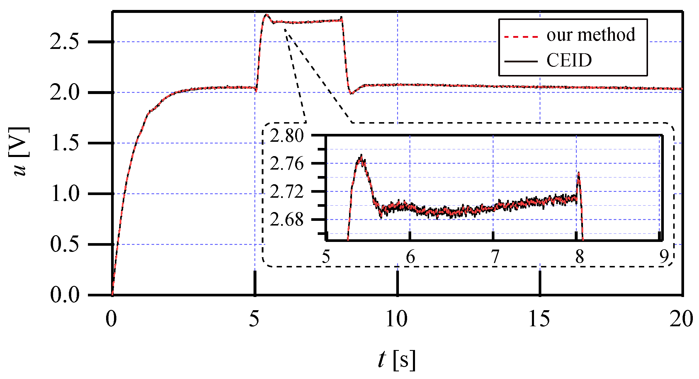
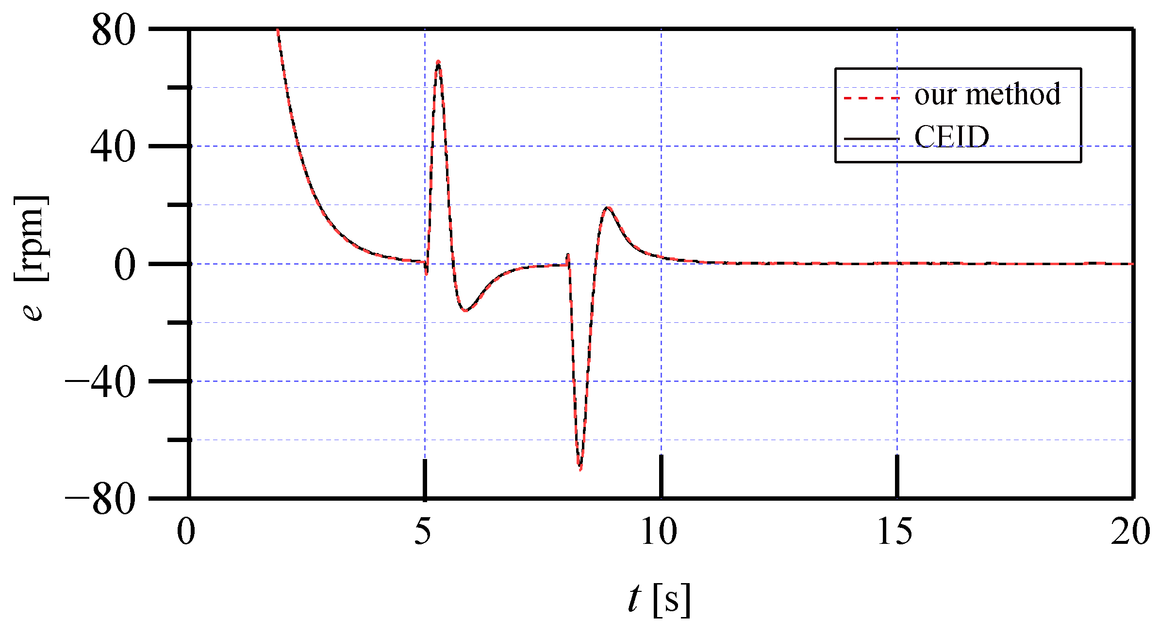
5. Simulation and Comparison Results

The system parameters of the plant described by
A = 8.807 4.225 0.4877 8 0 0 0 0.25 0 , B = 8 0 0 , B d = 12.94 5.88 6.072 , C = 7.328 31.71 3.969 T
are the same as [26] for the coupled rotational motor system.
To validate the effectiveness of the developed method, the nonlinearity f ( x ) is chosen as [27]
f ( x ) = 0 sin ( x 1 ) sin ( x 2 ) 0 T .
The lumped disturbance is given by
d ( t ) = 5 , 0 s < t < 8 s 0 , others .
The measurement noise v ( t ) is added by the Band-Limited White Noise module in MATLAB R2024a and is shown as Figure 2.
Set the reference as
r ( t ) = 1000 [ r / min ] .
Then, for the asymptotic tracking of the reference r ( t ) , set A R = 0.0001 and B R = 1 .
Commonly, F ( s ) is designed as a first-order low-pass filter and is selected here as
A F = 2.9 , B F = 2.5 , C F = 1 .
The linear quadratic regulation (LQR) method [28] is utilized to design observer gains for its simplicity, and it is utilized here to choose control parameters ( K p , K R ) , L, and K s .
Let a part of A ¯ in (44) be
A = A K B K R B R C A R .
Rewrite A as
A = A 0 B R C A R + B 0 K p K R .
Treat [ K p , K R ] of (63) as a state-feedback control gain [26]; then, we use the LQR method to select corresponding tunable matrices as follows:
Q 1 = 10 7 × diag { 1 , 1 , 1 , 100 } R 1 = 1
where diag presents the diagonal matrix. Then, K p = [ 0.0215 , 0.0227 , 0.0034 ] and K R = 0.0032 .
Likewise, the corresponding tunable matrices are selected as
Q 2 = 100 × diag { 1 , 1 , 1 } R 2 = 1
for state observer gain L, and finally L = [ 4.8350 , 8.7458 , 4.2950 ] T .
The corresponding tunable matrices are chosen as
Q 3 = diag { 1 , 1 , 1 } R 3 = 1 ,
and then the steady-state Kalman filter gain is K s = [ 0.3107 ,   0.9355 ,   0.4339 ] .
The estimator gain K e is designed to balance the performance of the speed of disturbance estimation and sensitivity to measurement noise in the estimator, which is finally set to be 1.
For the reference of (60), the simulation input and output results are illustrated in Figure 3 and Figure 4 under the disturbance of (59), which shows the robustness and rapid response to disturbances.
The disturbance estimation is shown in Figure 5, which demonstrates the lumped compensation of the simulation. When there is no disturbance, the estimator only compensates the nonlinearity f ( x ) ; when the disturbance d ( t ) is imposed, the estimator estimates the EID of both f ( x ) and d ( t ) .
To show the advancement of our method, a CEID approach is compared with the developed method. For fairness, except for the Kalman filter part, all parameters of the CEID approach are the same as those of the developed one.
The tracking errors of both methods, as shown in Figure 6 and Figure 7, are nearly identical. However, the control input in the CEID method is more sensitive to measurement noise, which could increase the burden on the actuators. In contrast, by incorporating the known nonlinearity into the Kalman filter, our control scheme shows improved performance, demonstrating the effectiveness of the KF-EIDE approach.

6. Conclusions

This study proposed a steady-state Kalman filter integrated with the EID method to address disturbance rejection and state estimation in nonlinear systems. Unlike conventional approaches, the proposed control framework unifies disturbance rejection and noise attenuation by using prior knowledge of system nonlinearities and the steady-state Kalman filter gain. This design avoids complex time-varying gain while retaining robustness against disturbances and measurement noise. Furthermore, the Kalman gain is rigorously derived to obtain an optimal one with the close-loop stability guaranteed. From simulation and comparisons, our method shows an excellent disturbance rejection and noise attenuation performance compared with the CEID method, validating the effectiveness of the KF-EIDE control scheme. Future research will focus on extending the framework to handle coupled multivariable disturbances and experimental validation under real-world noise conditions.

Author Contributions

Conceptualization, P.Y.; funding acquisition, G.H.; methodology, X.Z.; project administration, L.H.; software, B.Z.; supervision, G.H. and P.Y.; validation, B.Z.; writing—original draft, X.Z.; writing—review and editing, G.H. All authors have read and agreed to the published version of the manuscript.

Funding

This work was funded by the National Key Research and Development Project under Grant 2024YFB4710100.

Data Availability Statement

The datasets from this paper are accessible through the corresponding author with a reasonable request.

Conflicts of Interest

Author Lianqiang Han was employed by the company Xi’an Modern Control Technology Research Institute. The remaining authors declare that the research was conducted in the absence of any commercial or financial relationships that could be construed as a potential conflict of interest.

References

  1. Gurauskis, D.; Przystupa, K.; Kilikevičius, A.; Skowron, M.; Matijošius, J.; Caban, J.; Kilikevičienė, K. Development and Experimental Research of Different Mechanical Designs of an Optical Linear Encoder’s Reading Head. Sensors 2022, 22, 2977. [Google Scholar] [CrossRef] [PubMed]
  2. Cheng, M.; Zhou, J.; Qian, W.; Wang, B.; Zhao, C.; Han, P. Advanced Electrical Motors and Control Strategies for High-quality Servo Systems—A Comprehensive Review. Chin. J. Electr. Eng. 2024, 10, 63–85. [Google Scholar] [CrossRef]
  3. Hu, K.; Ma, Z.; Zou, S.; Li, J.; Ding, H. Impedance Sliding-Mode Control Based on Stiffness Scheduling for Rehabilitation Robot Systems. Cyborg Bionic Syst. 2024, 5, 0099. [Google Scholar] [CrossRef] [PubMed]
  4. Tu, Y.H.; Wang, R.F.; Su, W.H. Active Disturbance Rejection Control—New Trends in Agricultural Cybernetics in the Future: A Comprehensive Review. Machines 2025, 13, 111. [Google Scholar] [CrossRef]
  5. Gu, X.; Ren, H. A Survey of Transoral Robotic Mechanisms: Distal Dexterity, Variable Stiffness, and Triangulation. Cyborg Bionic Syst. 2023, 4, 0007. [Google Scholar] [CrossRef]
  6. Sun, X.; Lin, X.; Guo, D.; Lei, G.; Yao, M. Improved Deadbeat Predictive Current Control With Extended State Observer for Dual Three-Phase PMSMs. IEEE Trans. Power Electron. 2024, 39, 6769–6782. [Google Scholar] [CrossRef]
  7. Chen, W.H.; Yang, J.; Guo, L.; Li, S. Disturbance-Observer-Based Control and Related Methods—An Overview. IEEE Trans. Ind. Electron. 2016, 63, 1083–1095. [Google Scholar] [CrossRef]
  8. Zhou, L.; Jia, F.; She, J.; Li, M.; Xiao, W. Parallel-Equivalent-Input-Disturbance-Approach-Based Spatial Repetitive Control for Rotating Systems. IEEE Trans. Ind. Electron. 2025; early access. [Google Scholar] [CrossRef]
  9. Zhu, Y.; Bao, Z.; Teng, H.; Yang, Y.; Cui, Y. Disturbance Separation-Based Enhanced Antidisturbance Attitude Control for Flexible Spacecrafts with Composite Disturbances. IEEE Trans. Ind. Electron. 2024, 71, 13146–13156. [Google Scholar] [CrossRef]
  10. Yin, X.; She, J.; Liu, Z.T.; Xiong, Y. Disturbance Suppression and System Design Based on Parallel-Equivalent-Input-Disturbance Approach. IEEE Trans. Syst. Man Cybern. Syst. 2023, 53, 3654–3665. [Google Scholar] [CrossRef]
  11. Yin, X.; Shi, Y.; She, J.; Wang, H. Equivalent Input Disturbance-Based Control: Analysis, Development, and Applications. IEEE Trans. Cybern. 2024, 54, 2654–2667. [Google Scholar] [CrossRef]
  12. She, J.H.; Fang, M.; Ohyama, Y.; Hashimoto, H.; Wu, M. Improving Disturbance-Rejection Performance Based on an Equivalent-Input-Disturbance Approach. IEEE Trans. Ind. Electron. 2008, 55, 380–389. [Google Scholar] [CrossRef]
  13. Yu, P.; Liu, K.; Li, X.; Yokoyama, M. Robust control of pantograph-catenary system: Comparison of 1-DOF-based and 2-DOF-based control systems. IET Control Theory Appl. 2021, 15, 2258–2270. [Google Scholar] [CrossRef]
  14. Khodarahmi, M.; Maihami, V. A Review on Kalman Filter Models. Arch. Comput. Methods Eng. 2022, 30, 727–747. [Google Scholar] [CrossRef]
  15. Bian, Y.; Yang, Z.; Sun, X.; Wang, X. Speed Sensorless Control of a Bearingless Induction Motor Based on Modified Robust Kalman Filter. J. Electr. Eng. Technol. 2023, 19, 1179–1190. [Google Scholar] [CrossRef]
  16. Yu, K.; Li, S.; Zhu, W.; Wang, Z. Sensorless Control Scheme for PMSM Drive via Generalized Proportional Integral Observers and Kalman Filter. IEEE Trans. Power Electron. 2025, 40, 4020–4033. [Google Scholar] [CrossRef]
  17. Knox, J.; Blyth, M.; Hales, A. Advancing state estimation for lithium-ion batteries with hysteresis through systematic extended Kalman filter tuning. Sci. Rep. 2024, 14, 12472. [Google Scholar] [CrossRef]
  18. Park, G. Optimal vehicle position estimation using adaptive unscented Kalman filter based on sensor fusion. Mechatronics 2024, 99, 103144. [Google Scholar] [CrossRef]
  19. Lei, T.; Hou, M.; Li, L.; Cao, H. A State Estimation of Dynamic Parameters of Electric Drive Articulated Vehicles Based on the Forgetting Factor of Unscented Kalman Filter with Singular Value Decomposition. Actuators 2025, 14, 31. [Google Scholar] [CrossRef]
  20. Sun, H.; Madonski, R.; Li, S.; Zhang, Y.; Xue, W. Composite Control Design for Systems With Uncertainties and Noise Using Combined Extended State Observer and Kalman Filter. IEEE Trans. Ind. Electron. 2022, 69, 4119–4128. [Google Scholar] [CrossRef]
  21. Yin, X.; She, J.; Wu, M.; Sato, D.; Ohnishi, K. Disturbance rejection using SMC-based-equivalent-input-disturbance approach. Appl. Math. Comput. 2022, 418, 126839. [Google Scholar] [CrossRef]
  22. Zhou, Y.; She, J.; Wang, F.; Iwasaki, M. A Model-Predictive-Enabled Equivalent-Input-Disturbance Approach for Disturbance Rejection. In Proceedings of the 2023 IEEE 6th International Conference on Industrial Cyber-Physical Systems (ICPS), Wuhan, China, 8–11 May 2023; pp. 1–5. [Google Scholar] [CrossRef]
  23. Žvirblis, T.; Pikšrys, A.; Bzinkowski, D.; Rucki, M.; Kilikevičius, A.; Kurasova, O. Data Augmentation for Classification of Multi-Domain Tension Signals. Informatica 2024, 35, 883–908. [Google Scholar] [CrossRef]
  24. Crassidis, J.L.; Junkins, J.L. Optimal Estimation of Dynamic Systems; Chapman and Hall/CRC: New York, NY, USA, 2004. [Google Scholar] [CrossRef]
  25. Sontag, E.D. Input to State Stability: Basic Concepts and Results. In Nonlinear and Optimal Control Theory; Springer: Berlin/Heidelberg, Germany, 2008; pp. 163–220. [Google Scholar] [CrossRef]
  26. Yu, P.; Wu, Q.; Liu, K.Z.; She, J.; Li, X. Tunable Nonlinear-Function-Based Estimators for Mismatched Disturbances and Performance Analysis. IEEE Trans. Ind. Electron. 2024, 71, 11453–11464. [Google Scholar] [CrossRef]
  27. Yin, X.; Shi, Y.; She, J.; Xie, M.; Wang, Z. Nonlinearity and Disturbance Compensation Based on Improved Equivalent-Input-Disturbance Approach. IEEE/ASME Trans. Mechatron. 2024, 29, 703–714. [Google Scholar] [CrossRef]
  28. Yu, P.; Liu, K.Z.; Liu, X.; Li, X.; Wu, M.; She, J. Robust Consensus Tracking Control of Uncertain Multi-Agent Systems With Local Disturbance Rejection. IEEE/CAA J. Autom. Sin. 2023, 10, 427–438. [Google Scholar] [CrossRef]
Figure 1. The control scheme of the KF-EIDE approach.
Actuators 14 00189 g001
Figure 2. The measurement noise v ( t ) in the simulation.
Actuators 14 00189 g002
Figure 3. The control input u ( t ) of the simulation under the KF-EIDE approach.
Actuators 14 00189 g003
Figure 4. The control output y o ( t ) of the simulation under the KF-EIDE approach.
Actuators 14 00189 g004
Figure 5. The disturbance estimation d ˜ e ( t ) of the simulation with the KF-EIDE approach.
Actuators 14 00189 g005
Figure 6. The control inputs u ( t ) of the simulation using the CEID and our method.
Actuators 14 00189 g006
Figure 7. The tracking errors of e ( t ) = r ( t ) y o ( t ) of the simulation using the CEID and our method.
Actuators 14 00189 g007
Disclaimer/Publisher’s Note: The statements, opinions and data contained in all publications are solely those of the individual author(s) and contributor(s) and not of MDPI and/or the editor(s). MDPI and/or the editor(s) disclaim responsibility for any injury to people or property resulting from any ideas, methods, instructions or products referred to in the content.

