Article

Real-Time Data-Driven Method for Bolt Defect Detection and Size Measurement in Industrial Production

Department of Mechanical Engineering, Inha University, Incheon 22212, Republic of Korea
*
Author to whom correspondence should be addressed.
Actuators 2025, 14(4), 185; https://doi.org/10.3390/act14040185
Submission received: 28 February 2025 / Revised: 31 March 2025 / Accepted: 8 April 2025 / Published: 9 April 2025

Abstract

:
To enhance the automatic quality monitoring of bolt production, YOLOv10, Intel RealSense D435, and OpenCV were integrated to leverage GPU parallel computing capabilities for defect recognition and size measurement. To improve the model’s effectiveness across various industrial production environments, data augmentation techniques were employed, resulting in a trained model with notable precision, accuracy, and robustness. A high-precision camera calibration method was used, and image processing was accelerated through GPU parallel computing to ensure efficient and real-time target size measurement. In the real-time monitoring system, the average defect prediction time was 0.009241 s, achieving an accuracy of 99% and demonstrating high stability under varying lighting conditions. The average size measurement time was 0.021616 s, and increasing the light intensity could reduce the maximum error rate to 1%. These results demonstrated that the system excelled in real-time performance, accuracy, robustness, and efficiency, effectively addressing the demands of industrial production lines for rapid and precise defect detection and size measurement. In the dynamic and variable context of industrial applications, the system can be optimized and adjusted according to specific production environments and requirements, further enhancing the accuracy of defect detection and size measurement tasks.

1. Introduction

The human visual cortex processes visual information by receiving signals from the retina, enabling the observation, identification, and differentiation of objects. In the realm of artificial intelligence, artificial neural networks are employed to simulate human visual processing abilities [1,2]. Computational models that emulate neural networks form deep learning, specifically artificial neural networks (ANNs) [3,4,5]. The deep learning umbrella encompasses various computational frameworks, including convolutional neural networks (CNNs) [6] and recurrent neural networks (RNNs) [7], with CNNs specifically designed to replicate the structure of the visual cortex. As deep learning has advanced rapidly, the field of computer vision (CV) [8] has also progressed significantly, aiming to simulate human visual functions. The three core tasks in computer vision are image classification, object detection, and object segmentation. The achievement of these tasks typically relies on deep learning models, such as ResNet [9] for image classification, YOLO (You Only Look Once) [10,11] for object detection, and Mask R-CNN [12] for object segmentation.
The applications of artificial intelligence encompass various industries, including energy [13], security [14], healthcare [15], and education [16]. Notably, in the manufacturing sector, there is significant potential for automation and quality inspection through computer vision [17,18]. Traditional manual inspection methods often suffer from high error rates and low efficiency, making it challenging to detect scratches and cracks with the naked eye. In contrast, computer vision improves accuracy in these inspections. Key requirements for industrial inspection include rapid detection, high precision, multi-target detection, and efficient operation on constrained hardware. YOLO functions as a single-stage detector, allowing the model to perform all tasks (bounding box regression and classification) through a single forward propagation. This approach eliminates the need for candidate region generation and secondary classification, as seen in Faster R-CNN. Consequently, YOLO features a simpler structure, has faster training and inference speeds, and effectively meets the real-time monitoring requirements of high-speed automated production lines. The YOLO model, particularly its lighter versions such as YOLOv10, operates efficiently on devices with limited computational resources (e.g., edge devices or embedded systems). This efficiency allows for a balance between high precision and high performance with effective resource utilization. In complex industrial production environments, YOLO facilitates multi-target monitoring while maintaining high robustness and stability. Based on the aforementioned advantages and characteristics, YOLO demonstrates a broad spectrum of applications and efficient problem-solving capabilities in industrial detection, particularly in complex scenarios that necessitate real-time performance and precision. Consequently, the YOLO architecture has been selected to accomplish the task of real-time target monitoring.
The YOLO series of models has made notable advancements in the field of industrial defect detection. Wu et al. [19] proposed using K-means clustering to optimize candidate boxes, thereby enhancing the YOLOv3 algorithm. This approach achieved an accuracy of 93.5% in detecting defects in electrical connectors, surpassing both Faster R-CNN and the original YOLOv3, and satisfying industrial requirements. Yu et al. [20] utilized FPGA hardware acceleration to optimize the computational performance of the YOLO algorithm, addressing the real-time and efficiency challenges associated with visual defect detection in industrial contexts. Jung et al. [21] integrated YOLO (specifically YOLOv5) with ResNet models for the detection and classification of hot-pressing points, thereby enhancing both the efficiency and accuracy of quality inspections in automobile manufacturing. Li et al. [22] introduced the YOLO-RFF model, which employs deep separable convolution to reduce computational load, making it suitable for the industrial defect detection of steel and electronic components. Qi et al. [23] developed a product defect detection and classification system based on the YOLO framework, addressing the inefficiencies and inaccuracies of traditional quality inspection methods, which often fail to meet the demands of industrial automation. This system enabled real-time detection and significantly enhanced both detection efficiency and accuracy. Lastly et al. [24] applied the YOLO algorithm to detect welding surface defects, optimizing data processing and network structure, and successfully implementing it in surface quality control during the welding process. Improvements to the YOLO algorithm and its applications have enhanced detection efficiency and accuracy across various industries. However, existing studies primarily focus on specific industrial defects, such as welding and hot-pressing points, rather than addressing multi-target detection challenges encountered in real industrial production processes. Additionally, these studies often overlook the environmental impacts posed by complex industrial backgrounds, including variations in lighting and interference from surface reflections. Notably, there is a lack of research focused on the detection of bolt surface quality.
Bolts are one of the most used connection and fastening components in industrial equipment, machinery, and infrastructure. Defects in bolts can significantly reduce their load-bearing capacity and adversely affect the stability and service life of mechanical systems. In high-intensity applications, even small deviations or material defects can lead to equipment failure or catastrophic outcomes. Therefore, research on bolt size and defect detection utilizing deep learning techniques is essential. Among the YOLO model series, YOLOv10 offers higher detection accuracy, faster detection speed, and enhanced robustness, along with support for adaptive optimization. OpenCV [25,26], along with hardware like the Intel RealSense D435 and GPUs, enables efficient real-time image and video processing. These technologies are widely applied in various fields, including automated inspection, robotics, and intelligent monitoring for image acquisition. Compared to standard RGB cameras, the Intel RealSense D435 provides both RGB and depth data, maintaining stable data output even in low-light environments. Its infrared projector mitigates the impact of reflections on metal surfaces, enabling high-frame-rate real-time detection. Consequently, this study integrates YOLOv10, OpenCV, and the Intel RealSense D435 to leverage the real-time performance of YOLO, the powerful and user-friendly computer vision capabilities of OpenCV, and the depth information acquisition capabilities of the D435. This integration enhances the robustness and accuracy of detection in complex environments. The advantages of this study are significant. Existing research typically relies solely on RGB images for defect detection; however, this study innovatively enhances model robustness in low-light and complex backgrounds by incorporating depth information from the Intel RealSense D435. The integration of depth perception with the YOLOv10 model substantially improves the system’s adaptability in real industrial environments, allowing it to maintain high-precision detection even under challenging conditions, such as in the presence of reflections on metal surfaces. Furthermore, by optimizing and expanding the bolt defect detection dataset to include various bolt types, defect types, and diverse shooting angles and lighting conditions, this study not only enhances the model’s generalization ability but also ensures its wide applicability across different industrial scenarios. In contrast to the limitations of traditional fixed datasets, the diversity of this dataset offers a more accurate and flexible solution for industrial defect detection. Most existing studies, particularly those utilizing YOLO for target detection, primarily focus on testing with pre-existing image data, often neglecting real-time detection and verification. This study addresses this gap by conducting real-time detection tests on bolts, thereby ensuring the feasibility of the proposed solution.

2. Research Foundation

2.1. YOLO

In 2016, Joseph Redmon proposed a novel object detection method known as YOLO, which significantly transformed the approach to target detection. This approach replaced traditional classifier-based methodologies, instead framing target detection as a unified regression problem [27]. The entire detection process is executed in a single step, transforming the input image into output bounding box predictions and category probabilities using a single neural network. However, this method faces difficulties in effectively detecting small and densely packed targets. Following the initial development of YOLO, the primary objectives have focused on enhancing detection accuracy—particularly for small targets and in complex scenes—while also improving the efficiency and real-time performance of the grid structure and ensuring adaptability to various hardware environments. Table 1 summarizes the key advancements from YOLOv1 to YOLOv10. Compared to other models, YOLOv10 has undergone comprehensive optimization regarding detection performance, inference efficiency, training efficiency, and hardware adaptability, particularly compared to YOLOv8 and RT-DETR (Real-Time DEtection Transformer). Notably, the implementation of a Non-Maximum Suppression (NMS)-free design and lightweight enhancements has significantly improved the model’s real-time capabilities and its adaptability across multiple scenarios, establishing it as a leading solution in the realm of real-time target detection. NMS is a postprocessing algorithm utilized in target detection and computer vision tasks, primarily aimed at eliminating redundant candidate boxes.
The detailed network structure of YOLOv10 is illustrated in Figure 1. The primary innovations are described below.
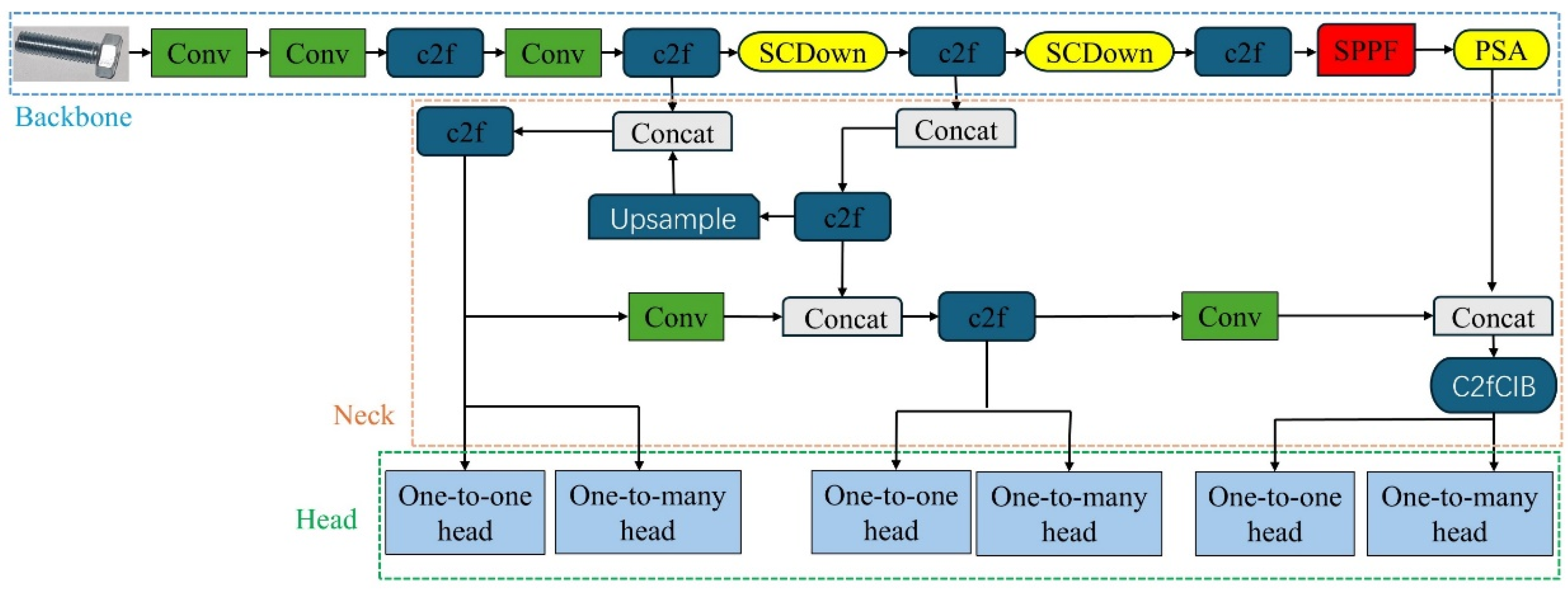
  • YOLOv10 utilizes an NMS training strategy and a consistent dual allocation strategy. The consistent dual allocation strategy refers to a method for optimizing feature allocation within the target detection framework. This approach ensures that both small and large targets can be effectively detected by maintaining consistency in target allocation across feature layers of varying scales and by employing a dual allocation mechanism. During the training process, multiple prediction boxes (Positive Predictions) are assigned to each ground truth (GT), implementing a one-to-many matching method (one-to-many head). This approach generates additional supervision signals during training, thereby enhancing both classification and localization capabilities. The one-to-one matching (one-to-one head) eliminates the necessity for NMS during the inference stage, resulting in the output of a singular prediction box. This significantly enhances inference efficiency and minimizes errors that may arise from redundant predictions and NMS. By employing consistent matching measurement formulas and hyperparameter adjustments, these two mechanisms can achieve synchronized optimization during the training phase.
  • Depthwise separable convolutions are utilized instead of traditional full convolution layers, along with lightweight classification heads, to alleviate computational and parameter burdens. Depthwise convolution facilitates spatial sampling from different regions, while pointwise convolution enables linear combinations within the channel dimension. This approach enhances feature representation capabilities, decouples downsampling operation, improves computational efficiency, and preserves more feature information.
  • Considering the high redundancy observed in the shallow stage, the CIB module is introduced. The CIB module enhances feature expression and discrimination capabilities through information compression and enhancement mechanisms, combining channel attention, depthwise separable convolution, and lightweight feature fusion. For the deeper stages, this module maintains sufficient expressive power while preventing excessive compression, thereby ensuring comprehensive feature extraction. Consequently, the overall performance of the model is enhanced while maintaining the integrity of feature extraction.
Figure 1. YOLOv10 network architecture diagram (note: CIB is Compact Information Block).
Actuators 14 00185 g001
Latency–accuracy and size–accuracy serve as critical indicators for comprehensively evaluating the performance and deployment adaptability of target detection models in practical applications. Latency refers to the time cost incurred by the model during the inference phase, which directly impacts real-time performance. In contrast to accuracy, latency illustrates the trade-off between speed and precision. Model size denotes the number of parameters or storage requirements of the model. When compared with accuracy, it assesses the model’s lightweight design capability. By concurrently evaluating these two indicators, one can gain a holistic understanding of the model’s practicality and deployment adaptability, aiding developers in achieving an optimal balance among accuracy, speed, and resource utilization. Wang, A. et al. [36] conducted a comparative analysis of YOLOv10 against YOLOv6-YOLOv9, PPYOLOE, RTMDet, YOLO-MS, Gold-YOLO, and RT-DETR. In addition to YOLO architectures, three mainstream target detection models, namely, PPYOLOE, RTMDet, and RT-DETR, were analyzed. The COCO dataset was employed for testing to evaluate the performance of various object detection models. The primary comparisons focus on the relationship between processing delay (speed) and average precision (AP) for each model, as well as the relationship between the number of parameters and average precision, as illustrated in Figure 2. According to Figure 2a, YOLOv10 achieves low-latency reasoning while maintaining high accuracy compared to the aforementioned three mainstream target detection models, fulfilling high-speed requirements and being suitable for real-time target detection scenarios. Figure 2b indicates that YOLOv10 maintains high accuracy with fewer parameters compared to the same models, achieving an effective balance between accuracy and model size. YOLOv10 has been optimized in terms of parameter count and exhibits a smaller model size, thus being lightweight. This framework strikes an efficient balance between accuracy and efficiency, reduces the requirements for computing resources and storage, effectively enhances reasoning speed, and meets real-time demands. The lightweight characteristic is particularly advantageous for deployment on devices with limited computing resources, such as mobile devices, embedded systems, and edge computing devices, while also reducing equipment costs. YOLOv11 and YOLOv12 represent optimized iterations within the YOLO series, showcasing advanced capabilities. However, model selection must prioritize actual usage, particularly in industrial deployments. Such deployments necessitate low computational resources and minimal power consumption; thus, lightweight models are preferred as they alleviate computational demands and facilitate integration into embedded systems, edge devices, and low-power GPUs or CPUs, thereby better addressing the real-time requirements of industrial production. While YOLOv11 enhances accuracy relative to Yolov10 through the incorporation of an attention mechanism, it incurs a reduction in inference speed, particularly when processing complex or large-scale backgrounds. This slowdown is especially pronounced in industrial settings with limited hardware resources. In contrast, YOLOv12 employs regional attention modules and a more hierarchical structure, resulting in significant improvements in accuracy and performance. However, this increase in model complexity necessitates robust computing resources and high-performance hardware support. For the real-time monitoring of bolt defects, YOLOv10 is more suitable for deployment on resource-constrained devices, enabling efficient real-time detection due to its streamlined architecture and lower computational requirements.

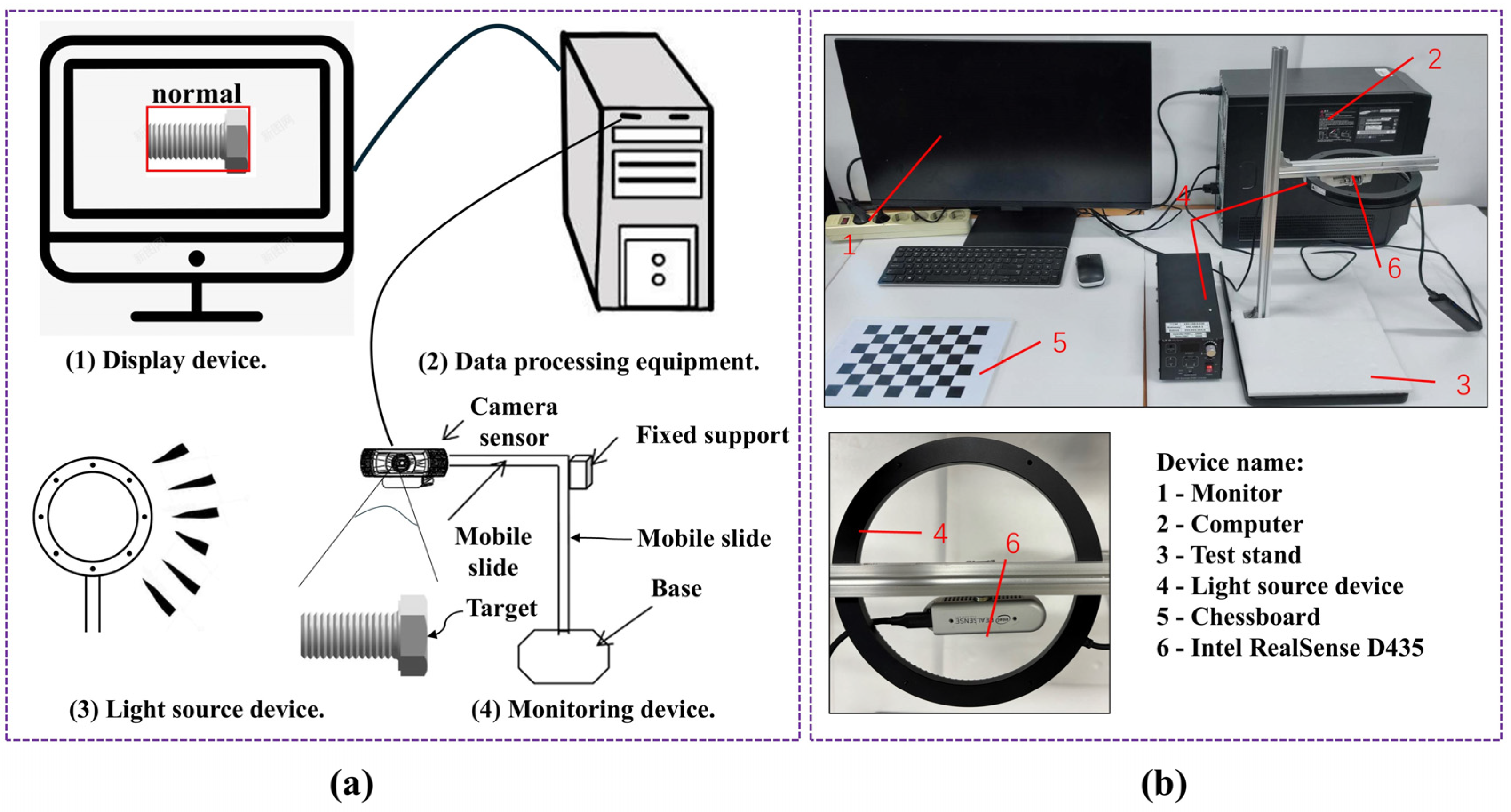
2.2. Intel RealSense D435

The Intel RealSense D435 is a versatile depth camera that employs stereo vision technology, with an optimal operating range of 0.3 to 3 m. It integrates an infrared sensor and an RGB camera to generate high-precision depth data alongside high-resolution color images, as illustrated in Figure 3. The left and right imagers capture infrared images, and the disparity data from these sensors are utilized to calculate depth information, thereby enabling accurate depth perception. Additionally, an infrared projector emits invisible infrared light patterns to improve performance in low-light conditions, allowing the camera to capture precise depth measurements on poorly lit or less textured surfaces, such as smooth walls. The RGB module captures color images at a resolution of 1920 × 1080 at 30 frames per second (fps). The depth camera offers a resolution of up to 1280 × 720 and can capture depth data at rates of up to 90 fps, ensuring high depth accuracy. This combined capability provides detailed depth and color data, making the D435 suitable for a wide range of applications that require precise 3D sensing and imaging.

3. Methods

3.1. Dataset

This study utilized the publicly available dataset “Screw Detection Test (v21)” provided by D. Beliuzhenko in 2024 [37]. This dataset, published on Roboflow, is specifically designed for detecting defects in screws and bolts, serving as a foundation for training and testing machine learning models focused on screw and bolt defect detection tasks. However, the uniform size and color of the bolts, along with the predominance of defects such as dents and scratches, may pose challenges for models trained on this dataset, as shown in Figure 4a,b. These models may struggle to detect defects beyond the categories included, thereby limiting their effectiveness in diverse industrial environments. Consequently, this database was utilized as a basis for further supplementation. To enhance the applicability of our study, we employed data augmentation techniques to expand the dataset. This expansion includes a greater variety of bolt types and sizes, as well as various defect types. By doing so, we aim to cover a broader range of both normal and defective bolt scenarios, thereby enriching the diversity of the dataset.
The application of data enhancement technology primarily aims to improve the adaptability of models within complex production environments, thereby enhancing their generalization ability and robustness to maintain stability during industrial production processes. Data enhancement is fundamentally based on actual application scenarios. To meet diverse market demands, various types of bolts must be produced, exhibiting differences in length, shape, and color. Additionally, there are significant variations in bolt defects encountered during actual production. In practice, due to the fixed position of the camera, angle discrepancies arise between detection targets located at different positions relative to the camera. Furthermore, the industrial production process involves substantial lighting, where distance and equipment occlusion can alter light intensity and direction. Different automated production lines also present considerable background variations. The use of various image acquisition devices, along with differing parameters such as focal length and exposure, can lead to significant discrepancies in the quality of the collected images. To effectively utilize the model, it is essential to simulate potential scenarios encountered in a quasi-real industrial environment and enhance data diversity through various technical means. The primary implementation methods include the following aspects:
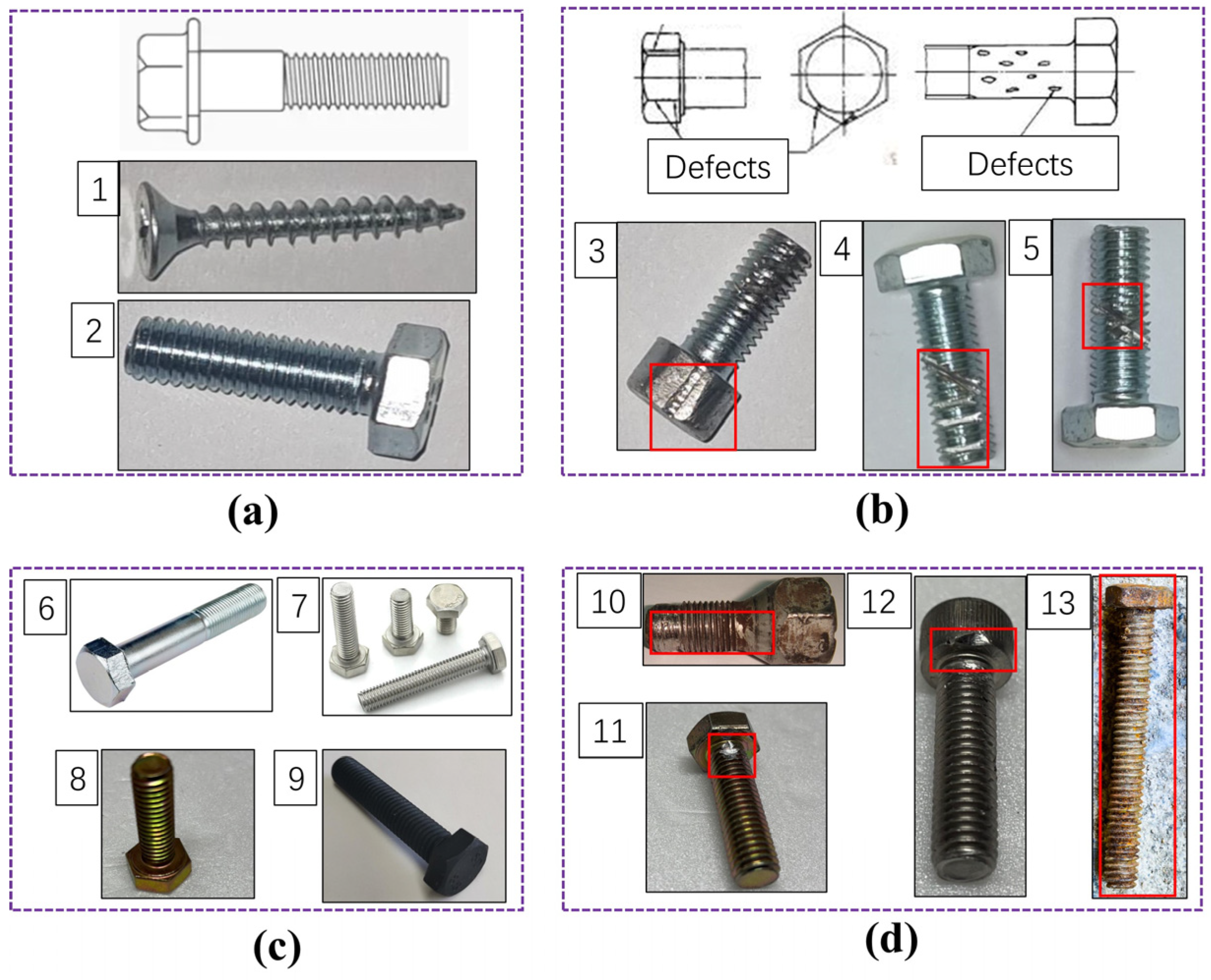
  • To address the impact of variations in bolt types, images of bolts with different colors and shapes were collected. The sizes of the bolts range from M4 to M45, thereby enhancing the diversity of the dataset.
  • Significant differences exist in the shapes of various bolt defect types. To monitor as many defective bolts as possible, it is essential to include a variety of defect types to enrich the database. In addition to the dents and scratches present in the original database, we added cracks, fractures, corrosion, and notches. The specific defect types and forms are detailed in Table 2.
  • Multiple variants were generated by altering the camera’s shooting angle (e.g., 45°, 90°, and 135°) to simulate the differences in image angles caused by positional variations during real-time detection. This approach aims to enhance the accuracy of model detection.
  • A fill light device was utilized to adjust light intensity and illumination direction, simulating the effects of light variations encountered in actual factory production processes. In the experiment, images with varying light intensities were collected, spanning a grayscale value range of 20 to 255, with increments of 20. The overall grayscale level range is from 0 to 255, where 255 indicates maximum intensity. This process aims to gather bolt image information under diverse lighting conditions, thereby improving the model’s stability and generalization ability across different lighting environments.
  • Given the significant variability in the surrounding environment during industrial production, it is essential to adapt to detection needs across various backgrounds. To achieve this, images were obtained against different backgrounds, including industrial production settings, engineering applications, and variations in background color. This strategy is intended to enhance the model’s adaptability in diverse production environments and bolster its robustness.
  • To improve the model’s adaptability to images captured by various camera devices, including standard RGB cameras, depth cameras, and mobile phone cameras with differing focal lengths and exposures, a comprehensive approach to bolt image collection was employed. These measures are designed to enhance data diversity and improve the model’s generalization ability.
Through data enhancement, a total of 412 bolt images of varying sizes, lighting conditions, colors, and backgrounds were obtained. This collection includes both normal and defective bolts, with defect types encompassing cracks, breakage, corrosion, and notches. When combined with the 2781 photos from the screw detection test training set, the final supplemented dataset comprises a total of 3193 bolt images, including 1286 normal bolts and 1607 defective bolts. During the training process, the division of datasets into training, validation, and test sets is fundamental to ensuring effective model training and evaluation. In scenarios involving relatively small datasets, it is beneficial to increase the proportion of the training set. This allows the model to learn from a sufficient number of samples, thereby capturing richer features and patterns. Consequently, the training set was allocated 90.6% of the data, amounting to 2893 images. To accommodate this increase, the proportions of the validation and test sets must be appropriately reduced. The validation set was set at 6.9% (220 images) to facilitate performance evaluation during training and parameter adjustment, and to mitigate overfitting. The test set was allocated 2.5% of the data, which is crucial for a fair assessment of the model’s generalization ability, as it does not participate in the training process.

3.2. Training Platform

We utilized an NVIDIA GTX 3060 GPU for training, configuring the image size to 640 × 640 pixels, the number of epochs to 200, and the batch size to 8. The Stochastic Gradient Descent (SGD) optimizer was employed, with the initial learning rate set to 0.01. The entire training process lasted a total of 2.931 h.

3.3. Performance Evaluation

Performance metrics are essential for assessing the accuracy and efficiency of object detection models, serving as a benchmark for their capability to identify and locate objects within images. Additionally, these metrics can enhance the model’s ability to manage false positives and false negatives, offering critical insights for evaluating and refining overall performance [38,39,40,41].
Precision = T P T P + F P
Recall = T P T P + F N
Accuracy = T P + T N T P + F P + T N + F N
where TP represents true positives, TN represents true negatives, FP represents false positives, and FN represents false negatives.
F 1 = 2 P r e c i s i o n R e c a l l P r e c i s i o n + R e c a l l
The F1 score is a more effective metric for evaluating the performance of imbalanced datasets, as it represents the harmonic means of precision and recall, thus offering a balanced assessment of both aspects. Additionally, evaluation metrics may include mean average precision (mAP). mAP is used to comprehensively evaluate the accuracy of the model at different recall rates.
Label distribution analysis is employed to optimize the dataset, ensuring fairness in training and enhancing the robustness of the model. Figure 5 presents the pair plot of bounding box attributes (x, y, width, and height) from the training dataset. The distribution characteristics and correlations of these bounding box attributes are examined through diagonal histograms and off-diagonal scatter plots.
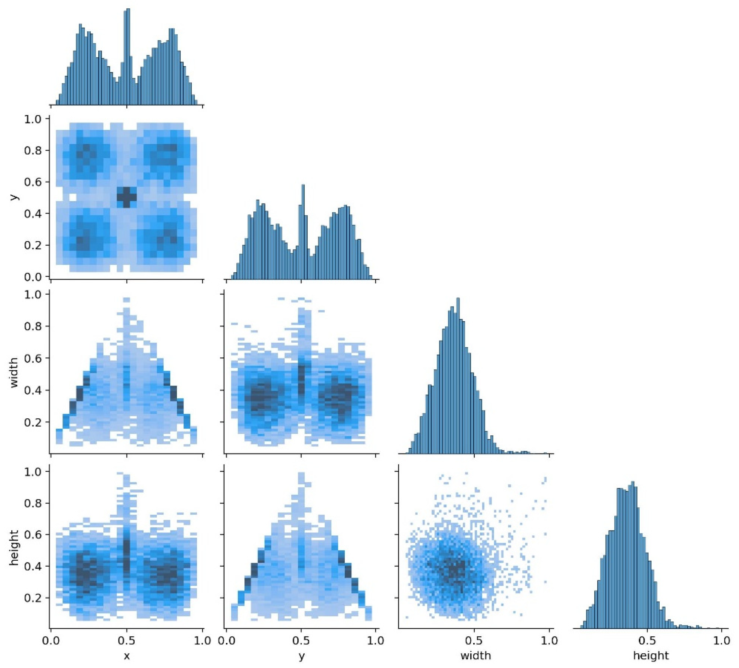
  • The histogram reveals that the x and y coordinates are evenly distributed across the image, indicating that the target locations cover the entire image area without bias toward any specific region. Conversely, the width and height histograms demonstrate that the sizes of most target boxes are concentrated in the medium-size range, with a slight concentration near the smaller sizes, as evidenced by the peak near the low end of the histogram.
  • The scatter plots of coordinates x and y are evenly distributed, further confirming that the objects are well distributed in both the horizontal and vertical directions of the image. The scatter plots of width against x and y coordinates exhibit a triangular distribution, while the scatter plots of height against x and y coordinates show a similar triangular pattern. This indicates a scarcity of objects with larger heights, with smaller heights being more prevalent. Additionally, the scatter plots of width and height reveal that smaller objects are concentrated, whereas larger objects are sparse. This suggests that the target size range in the training dataset is broad, but small and medium sizes are dominant.
  • The coordinates x and y are evenly distributed across the image, covering all areas and ensuring that the model can learn to detect targets at various locations. The distribution of width and height indicates that small- and medium-sized targets are predominant in the training set, while the number of large targets is limited.
Figure 5. Pair plot shows the distribution and relationships between the bounding box coordinates (x, y) and dimensions (width, height) in the training dataset.
Actuators 14 00185 g005
This dataset provides a solid foundation for bolt defect detection due to its uniform coordinate distribution, diverse target sizes, and proportional characteristics that align with actual needs. Consequently, the model trained on this dataset is well suited to meeting bolt detection requirements in industrial scenarios, particularly for tasks involving small- and medium-sized bolts and minor defects.
Figure 6a illustrates the variation in recall rate across different confidence thresholds. The recall rate approaches 1 at low confidence levels, indicating that the model can detect the majority of targets. Figure 6b presents the change in F1 score under varying confidence thresholds. Overall, the F1 curve remains close to 1, indicating that the model effectively balances precision and recall. The vertex of the curve represents the optimal F1 value and its corresponding confidence threshold, which is determined to be 0.308.
The training results are illustrated in Figure 7. All loss indicators, including box loss, classification loss, and distribution focal loss, exhibit a downward trend in both the training and validation sets. Notably, the validation loss closely approximates the training loss, suggesting that the model demonstrates strong learning and generalization capabilities in the regression and classification tasks associated with target detection. The model excels in both precision (as indicated by metrics/precision) and recall (as indicated by metrics/recall), achieving a high recall rate while maintaining substantial precision. Overall, the performance is well balanced, with no significant issues related to false detections or missed detections. The mean average precision at IoU (Intersection over Union) 0.50 (mAP50) increases rapidly and stabilizes at a high level, while the mAP50–95 curve is smoother, reflecting the model’s detection performance across various IoU thresholds. The continuous decline in the loss function signifies that the model training converges effectively, with no signs of overfitting. The precision, recall, and mAP curves collectively demonstrate that the model exhibits excellent detection performance.

3.4. Test

The trained model (best.pt) is utilized to evaluate the test set, which comprises 80 images. The testing process involves the following steps:
  • Each image in the test set is processed individually, with the total processing time recorded for each image, encompassing preprocessing, inference, and postprocessing phases;
  • The inference results are generated as visual images and subsequently stored in the designated output directory;
  • The categories and locations of the targets are extracted from the actual labels, which are then compared with the model’s detection results. This comparison allows for the quantification of errors in both classification and positioning, including instances of missed detections and false detections. The results are shown in Table 3.
The model comprises only 2.71 MB of parameters and exhibits a peak memory usage of 10.33 MB. This allows for deployment on mobile devices, embedded systems, edge computing devices, and other GPU-free embedded platforms. The average inference time per image on the CPU is 0.049 s (approximately 20 FPS), which is adequate for the detection requirements of automated production lines processing thousands of workpieces per minute. The model is characterized by efficient computing and real-time performance. With a lightweight model size of 5.5 MB, it is easily deployable on low-computing devices, significantly reducing hardware costs. The false alarm rate, defined as the proportion of actual targets that the model fails to detect, stands at 1.25%, indicating that most targets are accurately identified. The undetected defects are primarily due to occlusion; incomplete information in the defect images during the detection process adversely affects the model’s identification capabilities, leading to some defects being overlooked. To mitigate the false alarm rate, future datasets will include scenes with various occlusions of defects. Depending on the specific application scenario, this ratio may suffice to meet practical needs. The detection confidence ranges from 0.84 to 0.98, with the product defect box highlighting the suspected defect area. The model effectively captures complex details, and the detection box is accurately positioned, demonstrating a high level of certainty in classification results. In conclusion, the model is lightweight, efficient, and accurate, providing an effective solution for industrial automated detection and meeting the requirements for real-time bolt detection. Some prediction results are illustrated in Figure 8.

4. Real-Time Detection System Design and Testing
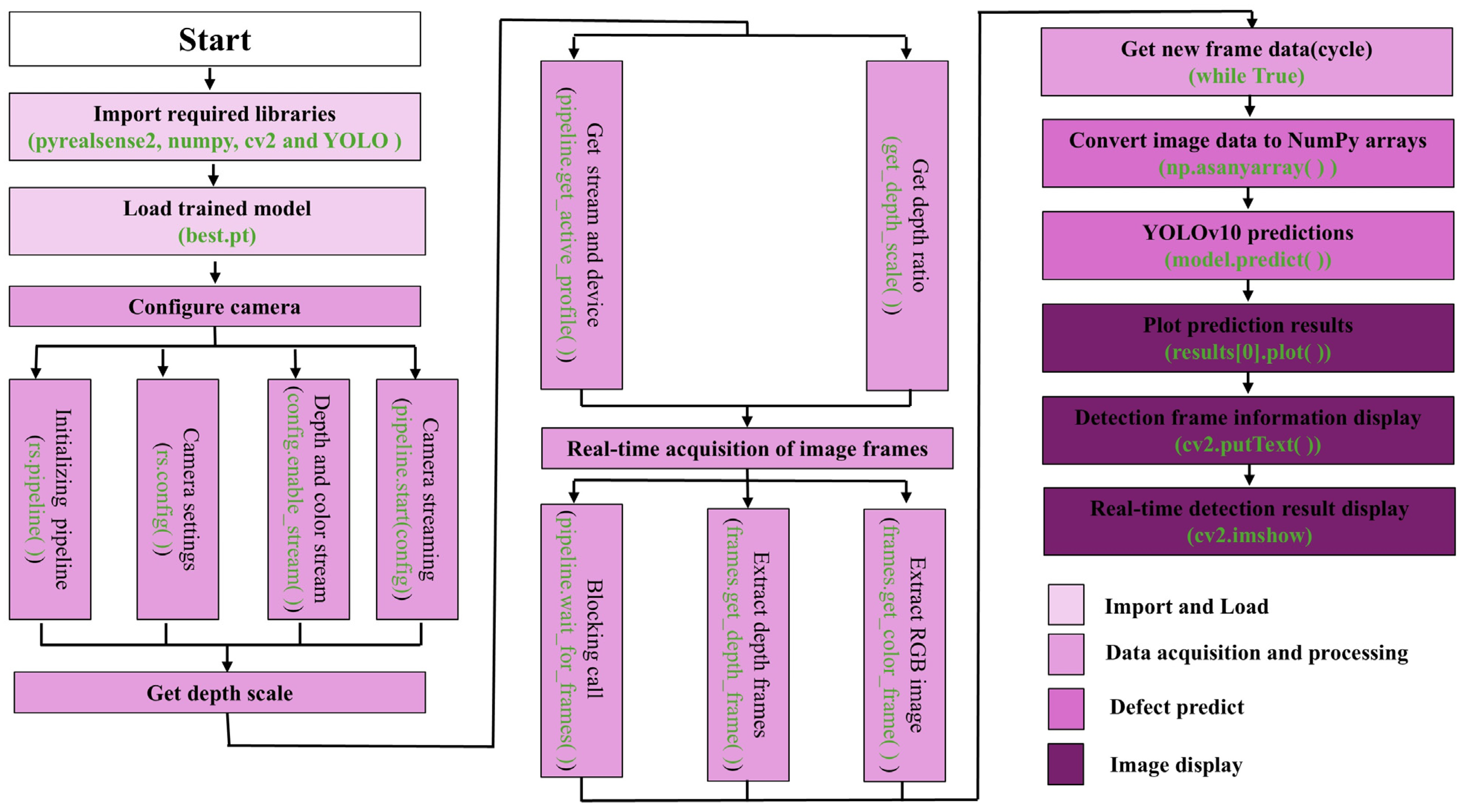
4.1. System Design

To facilitate the detection of bolt size and defects, a bolt detection system, as illustrated in Figure 9a, has been designed. This system primarily comprises a display device, a data processing device, a light source device, and a monitoring device. The display device is utilized to present monitoring results, including size and defect information, thereby streamlining the management of the inspection process. The data processing device consists of a dedicated computer that enhances image processing and analysis, enabling real-time processing and improving inspection accuracy. The light source device mimics the lighting conditions found in actual working environments, closely resembling the factory production setting. The inspection device primarily comprises a bracket and a camera, with an adjustable sliding mechanism that facilitates the modification of inspection height and position. This feature not only simplifies deployment but also ensures that the camera captures high-quality image data. An experimental test device has been constructed, as depicted in Figure 9b. The working computer is equipped with an Intel i7-8700 6-core CPU and an NVIDIA GeForce RTX 3060 GPU. The central processing unit (CPU) is produced by Intel Corporation, located in Santa Clara, CA, USA, while the graphics processing unit (GPU) is manufactured by NVIDIA Corporation, also based in Santa Clara, CA, USA. The light source device utilizes the EN-0212 controller for the lighting vision system (the gray value ranges from 0 to 255, with 255 representing the maximum). The gray value refers to the maximum value. The brightness of each pixel in a grayscale image ranges from 0 to 255, where 0 represents pure black and 255 represents pure white. The camera employed is the Intel RealSense D435. Each component is interconnected according to the data transmission interface requirements, and the remaining parts are processed and secured based on actual size specifications.

4.2. Size Measurement

4.2.1. Camera Calibration

Camera calibration [42] involves determining the internal and external parameters of a camera using mathematical models. The primary objective is to derive and compute the camera’s internal parameter matrix and distortion coefficients, aligning the image coordinate system with the actual world coordinate system to ensure the accuracy of the images and the reliability of depth information.
The camera calibration tool provided by ROS is utilized to calibrate the stereo camera (Intel RealSense D435). The Intel RealSense D435 is manufactured by Intel Corporation in Santa Clara, CA, USA. This method offers a high-precision, standardized calibration process that effectively eliminates distortion, reduces hardware configuration errors, enhances the robustness and stability of the system, and increases the reliability of stereo vision in various practical applications. Initially, an 8 × 6 chessboard grid is prepared, with each square having a side length of 0.025 m. Both the right and left cameras are activated, and the chessboard is moved (up and down, left and right, and rotated) according to the prompts. The corner points of the chessboard are identified and calibrated. Once sufficient data are collected, the calibration button is pressed, prompting the node to calculate the camera calibration parameters and obtain the intrinsic parameter matrix, distortion coefficients, and projection matrix, among other results, as shown in Table 4. The left camera’s focal lengths are fx = 442.8 and fy = 443.9, indicating that the focal lengths in the horizontal and vertical directions are closely aligned, and although the camera pixels are not perfectly square, they are very close. The principal point coordinates, cx = 441.7 and cy = 236.94, suggest that the principal point is near the center of the image. The distortion coefficient matrix reveals that both radial and tangential distortions are minimal. The rectangularization matrix, acting as the corrected rotation matrix, adjusts the imaging plane to remove distortion, ensuring the alignment of the left and right cameras’ fields of view. Following adjustments made through the projection matrix, the final corrected focal length is set to fx = fy = 529.3, while the position of the principal point (cx, cy) is slightly offset after correction to (623.6, 231.6). The parameters and adjustment result for the right camera are similar.

4.2.2. Measurement Method

The real-time object size measurement system based on the Intel RealSense camera is illustrated in Figure 10. To enhance the efficiency and performance of depth and RGB image processing, the system leverages the parallel computing capabilities of the GPU through data transmission, computing acceleration, and data return.
The measurement process can be described as follows:
1. For acquisition and alignment, the procedure is as follows: (1) The init_realsense() function initializes the RealSense camera by configuring the depth and RGB image streams with a resolution of 848 × 480 and a frame rate of 30 fps. This configuration utilizes rs.config() to set the resolution, frame rate, and format of the depth and color streams, ensuring efficient data capture. Subsequently, the camera pipeline is initiated to commence data streaming. (2) To address potential misalignment between depth and color data, the function employs rs.align() to ensure the spatial alignment of the depth and color images. Although the depth and RGB images are captured simultaneously, they may not always be spatially aligned due to the varying locations of the sensors. The alignment process in rs.align() rectifies this issue, ensuring that the depth measurements accurately correspond to specific color pixels, thereby providing synchronized and reliable data for further processing. (3) The pipeline.wait_for_frames() method is invoked to wait for and capture frames from the camera, while align.process(frames) guarantees that the frames are aligned. (4) Finally, the depth and color data are retrieved using depth_frame.get_data() and color_frame.get_data(), respectively, supplying the necessary information for tasks such as measurement and object detection. (5) The np.asanyarray() method is used to convert the image data into a NumPy array for further processing. Initially, the depth and color frames retrieved from the RealSense camera are not in NumPy array format. Converting them to NumPy arrays improves the efficiency and convenience of subsequent image processing operations such as edge detection.
2. For image preprocessing, the procedure is as follows: (1) RGB images are initially converted to grayscale images. This grayscale processing simplifies image data and reduces computational complexity by converting color images to grayscale. This conversion is achieved using the OpenCV function cv2.cvtColor(), which transforms the RGB (red, green, blue) channels into grayscale values, retaining only the brightness information of the pixels. (2) After conversion to grayscale, the image undergoes Gaussian blurring with the function cv2.GaussianBlur (gray, (7, 7), 0). The first parameter, (7, 7), specifies the size of the Gaussian kernel, while the second parameter, 0, indicates the standard deviation of the Gaussian kernel, which controls the degree of blur. (3) Edge detection is then performed using the cv2.Canny() method to extract the edges in the image. The resulting edge image undergoes dilation and erosion using cv2.dilate() and cv2.erode() to further enhance edge features.
3. For outlines and bounding boxes, the procedure is as follows: (1) The function cv2.findContours() is employed to detect contours in images processed through edge detection. These contours delineate the boundaries of objects or regions within the image and yield a list of contours that consist of a sequence of points defining the shape of each object. (2) Subsequently, cv2.minAreaRect() is utilized to compute the minimum bounding box surrounding each contour. This rectangular box is characterized by its center point, width, height, and angle, and serves to approximate the dimensions of the object represented by the contour. (3) Following this, perspective.order_points() reorganizes the corner points of the rectangle to ensure a consistent order (upper left, upper right, lower right, lower left), which is crucial for accurate geometric calculations and subsequent operations. (4) Finally, cv2.contourArea() determines the area of each contour and returns the pixel count contained within it, facilitating the exclusion of small, insignificant contours (e.g., those containing fewer than 100 pixels) to ensure that only relevant objects are processed.
4. For size calculation, the procedure is as follows: (1) The depth value of the rectangle’s center point is obtained by extracting depth information from the depth map through the depth_frame.get_distance() method, measured in meters and converted to millimeters. This depth information, along with the focal length and baseline length, is used to dynamically calculate the physical length per pixel (pixels per metric), which facilitates the conversion of pixel distances to actual physical sizes. In these industrial inspection environments, the object’s position is fixed or it is presented at a specific angle, minimizing the impact of perspective. Errors caused by factors other than the perspective effect are compensated for through depth calculations. (2) The actual physical size is dynamically calculated on the GPU using the calculate_pixels_per_metric_torch() method, which utilizes PyTorch for tensor calculations involving the depth map, focal length, and baseline. The actual object size (width and height) is computed using pixels_per_metric, which converts depth information and the physical size per pixel to yield the final dimensions in millimeters. (3) Additionally, the model uses torch.sqrt() to calculate the Euclidean distance between two points (such as opposite corners of the rectangle). PyTorch is a versatile deep learning framework that facilitates not only machine learning tasks but also efficient numerical computations. It represents data using tensors and leverages GPUs for acceleration, significantly enhancing the efficiency of large-scale computing tasks.
5. For results, the procedure is as follows: (1) The computed metrics (width, height, depth, pixels/unit, etc.) are recorded in a CSV file for further analysis and documentation. (2) The detected contours are rendered using cv2.drawContours(), and the measurement results are overlaid on the image with the cv2.putText() method. (3) All measurement outcomes are displayed in real time within the cv2.imshow() window.
Three sizes of bolts were selected for testing, with the results from tests conducted without external light sources illustrated in Figure 11. The measurement times for Test 1, Test 2, and Test 3 were 0.021319 s, 0.020833 s, and 0.021314 s, respectively, indicating a rapid measurement process at the millisecond level that meets the requirements for real-time monitoring. The measurement results showed a maximum error of 1.45 mm and a minimum error of 0.06 mm. Given the small range of measurement errors and the variability in bolt sizes, these errors are considered to be within a reasonable range.

4.2.3. Evaluation and Result Analysis

To accurately determine the measurement error, 100 bolts of varying sizes (with lengths ranging from 34.65 mm to 139.03 mm) were selected and measured without the use of an external light source. The measurement method involves sequentially placing individual bolts on the inspection base and measuring their dimensions. The actual sizes are determined using a vernier caliper with an accuracy of 0.01 mm, and the measurement results are recorded in order. The average measurement time was 0.021616 s. For statistical convenience, the error rate of the measurements was calculated based on the length dimension. The results are presented in Figure 12. As shown in Figure 12a, the error range of the measurement system was between −1.39 mm and +1.54 mm, with the majority of measurement errors concentrated around zero, indicating that the model can perform relatively accurate measurement in most instances. During the testing process, the error rate exhibited some fluctuations, reaching up to 4%, as shown in Figure 12b, which was associated with the varying sizes and shapes of the bolts. The measurement method demonstrated effectiveness without an external light source, with the error remaining within an acceptable range. The average measurement time of 0.021616 s reflects high efficiency, making it suitable for rapid detection in large-scale production environments. The short measurement duration is a significant advantage for industrial production and can enhance production line efficiency.
To evaluate the model comprehensively, we combined the measurement results from five groups exposed to different light intensities. The testing method was consistent with that used for the no-light group. The light intensities (gray values) were set at 50, 100, 150, 200, and 255, respectively. Gray values range from 0 to 255, with 255 representing the maximum. For each group, the maximum and average error rates were calculated, and the results are presented in Table 5. A fixed exposure was employed during the tests, which helped mitigate variations in image quality caused by light fluctuations, thereby enhancing the stability and robustness of the system in variable lighting conditions. Analysis revealed that the average relative error decreased from 1.1% to 0.41%, while the maximum relative error fell from 4% to 1%. This indicates that increased light intensity can enhance measurement accuracy and minimize errors. Higher light intensity improves signal quality, reduces noise interference, and enhances imaging quality, which collectively contribute to improved measurement accuracy and decreased relative measurement errors. The robustness of the system has been validated through experiments, demonstrating that it maintains high accuracy even under significant light variations. In practical industrial applications, increasing the intensity of the light source can further enhance the stability and reliability of the system.

4.3. Defect Detection

4.3.1. Defect Detection Test and Analysis

The defect detection process integrates the Intel RealSense D435 camera with the YOLOv10 model to facilitate real-time target detection and depth information extraction, as illustrated in Figure 13. Initially, the camera captures frame data from both the depth and color streams using the pyrealsense2 library. During camera configuration, it is essential to enable both the depth and color streams, setting the resolution to 640 × 480 and the frame rate to 30 FPS. The depth scale of the sensor is obtained via the get_depth_scale () function and is subsequently converted into actual distance units. Continuous depth and color frames are acquired using pipeline.wait_for_frames(), with the frames converted into NumPy arrays within a loop. The resulting color image is then fed into the YOLO model for inference on the GPU, utilizing the model.predict() function to process the image. Finally, the processed image is displayed in real time through OpenCV’s cv2.imshow() function, allowing for the convenient observation of the defect detection results.
A total of 100 bolts were selected for defect detection, including 90 normal bolts and 10 defective bolts. The detection method involved placing the bolts directly on the substrate of the detection system for real-time analysis, while recording key information such as detection time and results. The defective bolt is illustrated in Figure 14a, with some prediction results displayed in Figure 14b. The detection results indicate that all 90 normal bolts were accurately identified, while 9 out of the 10 defective bolts were detected, resulting in 1 defective bolt being missed (misclassified as normal). The missed detection can be attributed to the defect’s location at the bolt head, which was angled relative to the detection platform, causing partial occlusion and hindering detection. The placement method is based on the actual conditions of industrial production. During the testing process, the defect side of the bolt is positioned upwards as much as possible when placed on the inspection platform to appear within the field of view (placed only once). However, in some cases, due to the camera angle, it is not possible for the entire bolt to appear within the field of view. Consequently, the model’s accuracy is reported to be 99%, suggesting that the majority of samples were correctly classified. The precision rate is 100%, indicating that nearly all predictions aligned with the actual defects. The recall rate stands at 90%, signifying that most defective bolts were accurately detected. The F1 score is calculated to be 94.7%. The false detection rate is 0%, while the missed detection rate is 10%. Based on these results, the model’s performance can be deemed robust. Furthermore, the average prediction time of the model is 0.009241 s, demonstrating strong real-time detection capabilities. Overall, the model performs effectively in the bolt defect detection task. Although the missed detection rate is slightly elevated, the accuracy and false detection rate are commendable. The model exhibits strong practical application potential. However, for actual implementation, it is advisable to further optimize the dataset and incorporate a wider variety of defective bolt samples to better align with real-world requirements.

4.3.2. Influence of Lighting Changes on Model Performance

The purpose of comparing the changes in model prediction confidence under varying grayscale values is to evaluate and optimize the model’s performance across different lighting conditions, thereby ensuring its reliability and stability in practical applications. The test method involves using the same bolt while maintaining consistent conditions, with the sole variable being the light intensity, represented by gray values. The gray value ranges from 0 to 255, with 255 representing the maximum. The values are set at 0, 5, 10, 15, etc., up to 255.0. A fixed-exposure method was still used in the testing to reduce image quality variations caused by fluctuations in lighting, thereby improving the system’s stability and robustness in dynamic lighting environments. Key metrics, including confidence levels and prediction results, were recorded for each group. At lower grayscale values (indicating weaker lighting), the model’s confidence is approximately 0.75. Under lower lighting conditions, the model exhibits a low level of confidence in detecting defective bolts, although it remains relatively stable. As the grayscale value increases (indicating enhanced light intensity), the confidence gradually rises and tends to stabilize. Beyond a grayscale value of about 50, the confidence rapidly approaches 0.9 and remains stable. Under stronger lighting, the model demonstrates higher detection confidence, leading to the increasingly stable identification of defective bolts. Once the grayscale value reaches a certain intensity (approximately 80 and above), the confidence remains nearly constant with minimal fluctuation. The specific value changes are shown in Figure 15. The system’s robustness was validated in the experiment, especially under conditions of significant lighting variation, where it still maintained high accuracy. Under strong lighting conditions, the model can reliably identify defective bolts without being significantly affected by the lighting intensity. Overall, these results indicate that appropriately increasing lighting can enhance the model’s detection confidence.
Leveraging the advantages of GPUs for processing parallel computing-intensive tasks, along with the robust capabilities of OpenCV in computer vision and image processing, and the exceptional performance of YOLOv10 in enhancing accuracy and accelerating inference, the D435 camera captures video streams and depth information to facilitate real-time dimensional measurement and defect detection. The test results indicate that the measurement time is reduced to a millisecond level while preserving high precision and accuracy. Furthermore, the model demonstrates stability under varying light intensities, which can reduce the impact of lighting changes in complex industrial production environments.

5. Conclusions

To enhance the automatic monitoring of bolt production, it is crucial to improve the quality control of bolts and reduce the risk of equipment failure or safety incidents due to size discrepancies or defects. Leveraging the superior detection accuracy, faster processing speed, and increased robustness of YOLOv10, in conjunction with the Intel RealSense D435 and GPU, allows for the effective utilization of depth information and target detection capabilities. This combination significantly enhances accuracy, robustness, and real-time performance in various tasks, including target detection, defect identification, and size measurement. Furthermore, integrating OpenCV with compatible hardware such as the Intel RealSense D435 and GPU facilitates efficient and real-time image and video processing tasks. To ensure high-precision and efficient detection, data augmentation, model training, defect detection testing, and size measurement testing were performed. The results indicate the following:
  • To enhance data quality, addressing the issue of data uniformity within the original dataset, as well as incorporating a greater variety of bolt types and defect categories, can facilitate the model’s ability to learn more nuanced features. This, in turn, enhances its recognition capabilities for various bolt types and defect manifestations, thereby improving the model’s generalization ability, accuracy, and robustness. These improvements were crucial for overcoming the variability associated with different bolt types and defects, ensuring the model’s effectiveness across diverse industrial production environments.
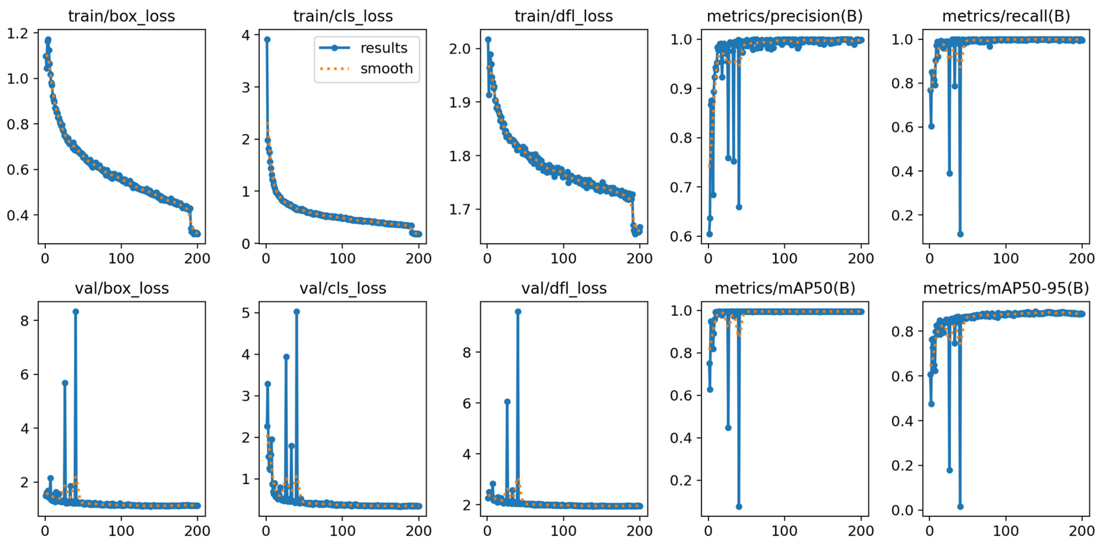
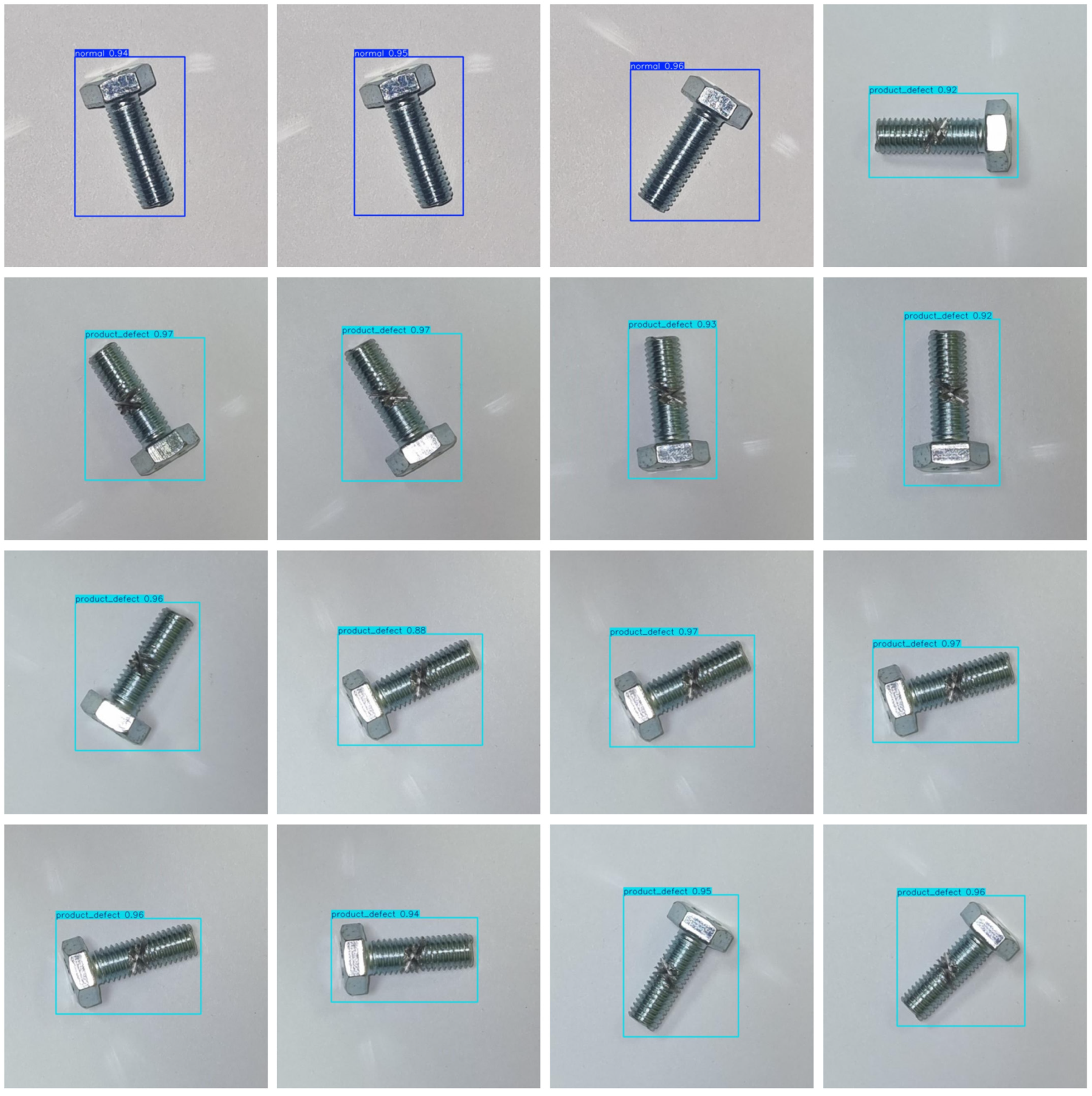
  • For the training and testing of the defect detection model, the data distribution was appropriate, and the model demonstrated a strong balance between precision and recall, as indicated by an F1 score that approaches 1. The optimal F1 value was reached at a confidence level of 0.308, where both precision and recall remain stable. The average inference time was 0.049 s, with a missed detection rate of 1.25%. The detection confidence exhibited a high range (0.84 to 0.98), allowing for the accurate capture of details related to bolt defects.
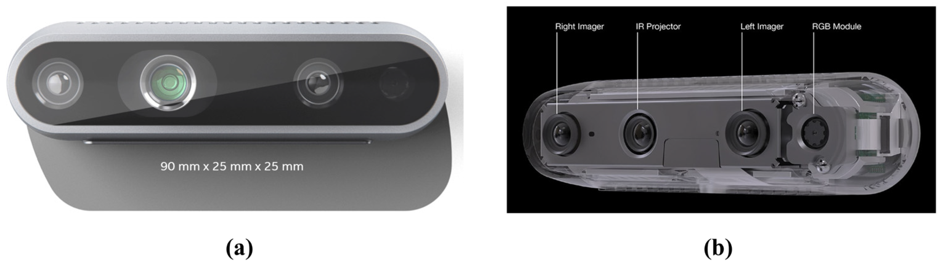
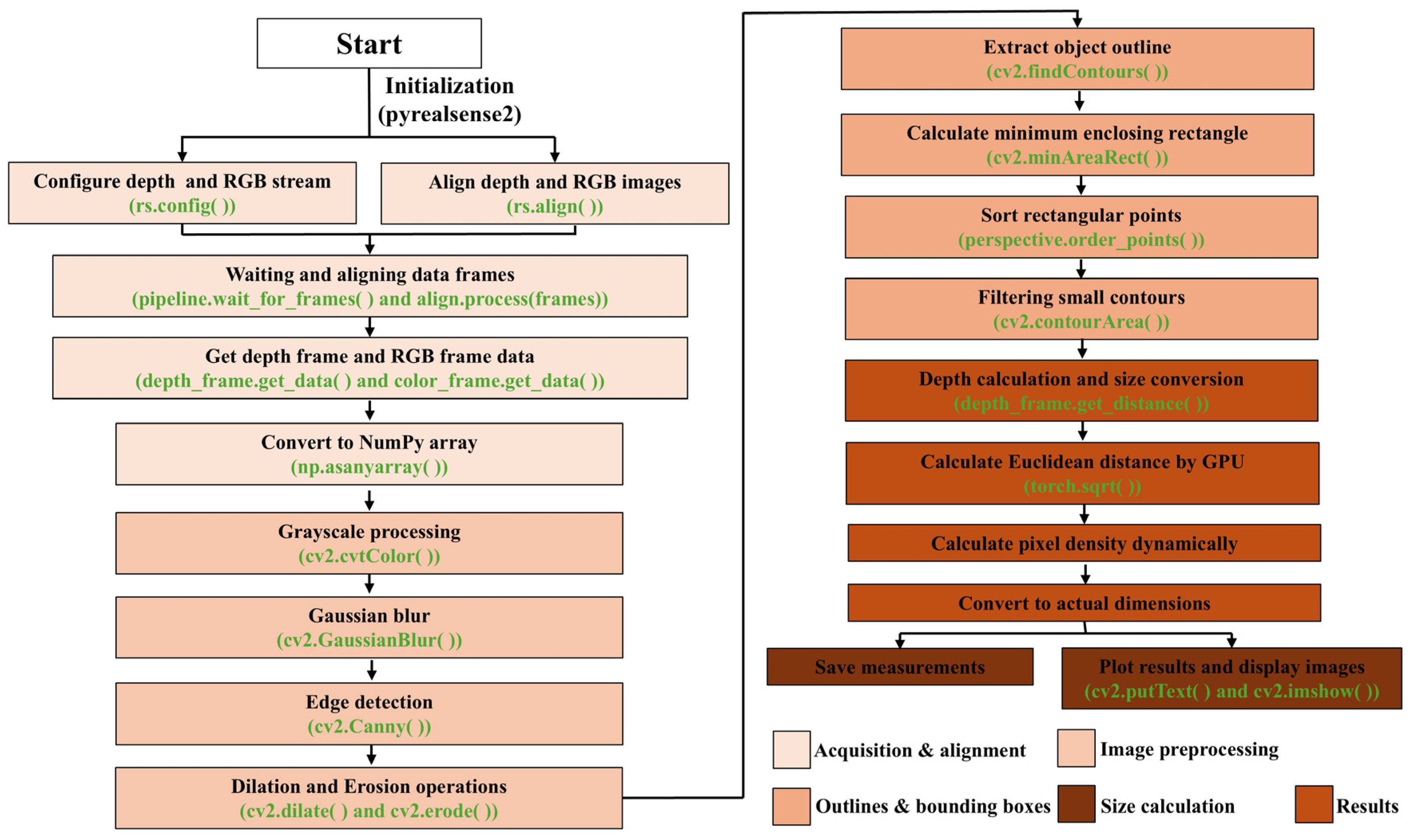
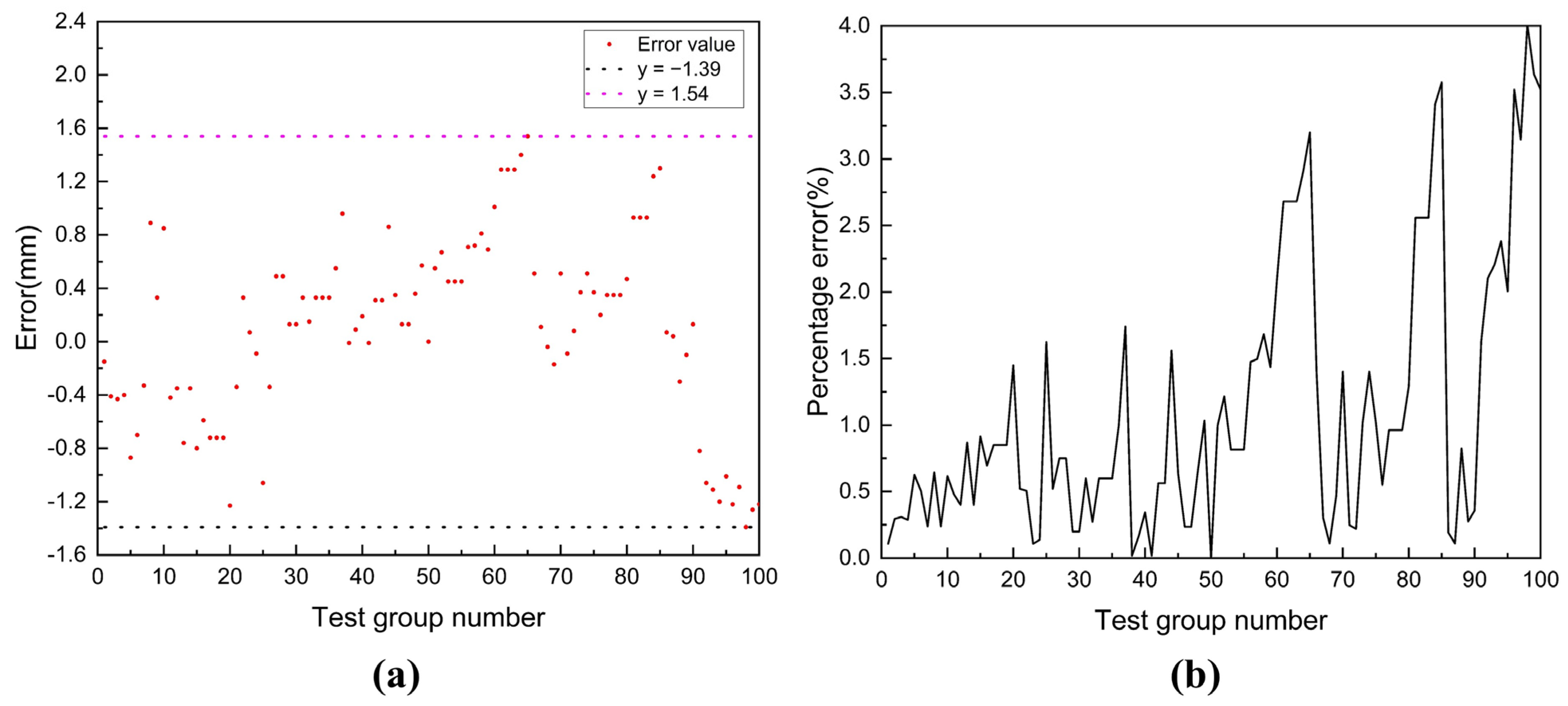
  • Based on the Intel RealSense D435 binocular camera, a high-precision camera calibration method was employed, and image processing was accelerated through GPU parallel computing to ensure efficient and real-time target size measurement. The test results indicated that the average measurement time was merely 0.021616 s, with an overall error range of −1.39 mm to +1.54 mm, and an error fluctuation of 4%. To evaluate the model more comprehensively, we calculated the average relative error rate, which decreased from 1.1% to 0.41%, and the maximum relative error rate, which dropped from 4% to 1%, under varying light intensities. Increasing the light intensity enhances signal quality, reduces noise interference, and improves image quality, thereby increasing measurement accuracy and decreasing relative measurement errors.
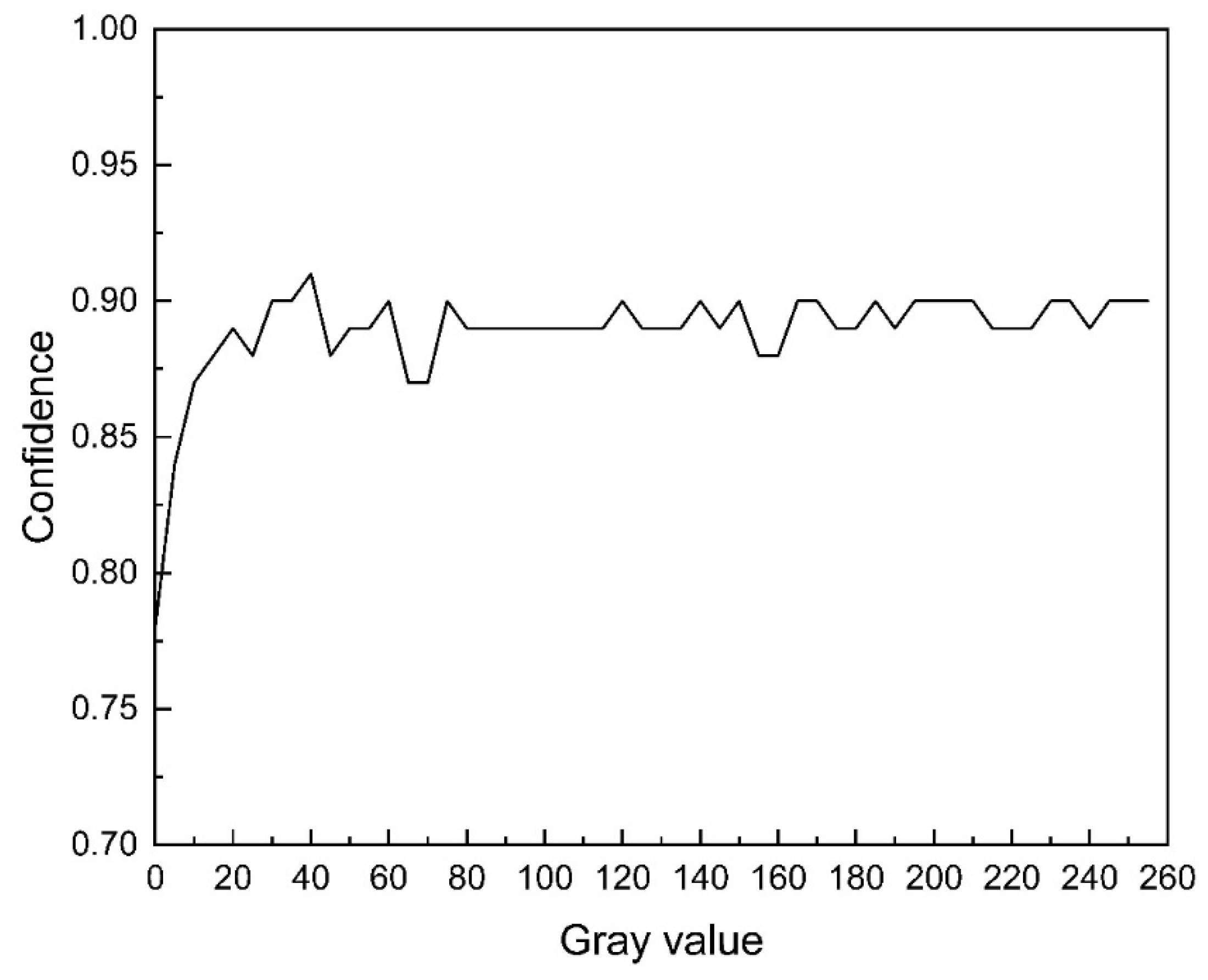
  • The combination of the Intel RealSense D435 depth camera and the YOLOv10 model enables efficient real-time target detection and defect recognition. Among the 100 test bolt samples, the model achieved an accuracy of 99%, a recall of 90%, and an F1 score of 94.7%. It demonstrated strong performance in detecting most defective bolts while effectively balancing precision and recall. With the use of GPU parallel computing, the average prediction time was 0.009241 s, showcasing excellent real-time processing capabilities. Furthermore, the model exhibits high stability under varying lighting conditions; as the lighting intensity increases, the confidence level gradually rises and stabilizes above 0.9. Given these results, the model is well suited for rapid defect detection tasks in industrial environments.
The bolt detection method based on YOLOv10 and the Intel RealSense D435 camera demonstrates strong performance in terms of real-time processing, accuracy, robustness, and efficiency, effectively fulfilling the requirements of industrial production lines for rapid and precise defect detection and dimensional measurement. This methodology has the potential for application in various industrial sectors, including welding quality inspection, product surface quality assessment, and circuit board connection verification. Notably, as deep learning continues to advance and GPU computing power improves, the integration of multiple sensors can facilitate the real-time health monitoring of production processes. Furthermore, a more lightweight model can be adapted for deployment on a wider range of embedded devices to satisfy diverse detection needs.

Author Contributions

Conceptualization, J.Y. and C.-H.L.; content preparation, J.Y.; writing—original draft preparation, J.Y.; writing—review and editing, J.Y. and C.-H.L.; supervision, C.-H.L. All authors have read and agreed to the published version of the manuscript.

Funding

This research received no external funding.

Data Availability Statement

The dataset is available upon request from the authors. The authors will provide the raw data supporting the conclusions of this article upon request.

Acknowledgments

This research was supported by a grant (2025-MOIS35-005) from Policy-linked Technology Development Program on Natural Disaster Prevention and Mitigation funded by Ministry of Interior and Safety (MOIS, Republic of Korea).

Conflicts of Interest

The authors declare that they have no known competing financial or nonfinancial interests or personal relationships that could have appeared to influence the work reported in this paper.

Abbreviations

ANNsArtificial Neural Networks
CNNsConvolutional Neural Networks
RNNsRecurrent Neural Networks
CVComputer Vision
YOLOYou Only Look Once
R-CNNRegion-Based Convolutional Neural Network
PPYOLOEPaddle Paddle You Only Look Once—Efficient
RTMDETReal-Time Multi-Scale Detector
YOLO-MSYou Only Look Once—Multi-Scale
Gold-YOLOGradient Optimization Learning-Based Dynamic YOLO
NMSNon-Maximum Suppression
SPFFSpatial Pyramid Pooling Fusion
FPSFrames Per Second
PGIProgressive Gradient Integration
GELANGlobal Enhancement Local Attention Network
GTGround Truth
CIBCompact Information Block
SGDStochastic Gradient Descent
IoUIntersection over Union
TPTrue Positives
TNTrue Negatives
FPFalse Positives
FNFalse Negatives
mAPMean Average Precision
ROSRobot Operating System

References

  1. Kriegeskorte, N. Deep neural networks: A new framework for modeling biological vision and brain information processing. Annu. Rev. Vis. Sci. 2015, 1, 417–446. [Google Scholar] [CrossRef] [PubMed]
  2. Korteling, J.E.H.; van de Boer-Visschedijk, G.C.; Blankendaal, R.A.M.; Boonekamp, R.C.; Eikelboom, A.R. Human-versus artificial intelligence. Front. Artif. Intell. 2021, 4, 622364. [Google Scholar] [CrossRef]
  3. Zupan, J. Introduction to artificial neural network (ANN) methods: What they are and how to use them. Acta Chim. Slov. 1994, 41, 327. [Google Scholar]
  4. Han, S.H.; Kim, K.W.; Kim, S.; Youn, Y.C. Artificial neural network: Understanding the basic concepts without mathematics. Dement. Neurocogn. Disord. 2018, 17, 83–89. [Google Scholar] [CrossRef]
  5. Deng, L.; Wu, Y.; Hu, X.; Liang, L.; Ding, Y.; Li, G.; Xie, Y. Rethinking the performance comparison between SNNS and ANNS. Neural Netw. 2020, 121, 294–307. [Google Scholar] [CrossRef]
  6. Song, J.; Gao, S.; Zhu, Y.; Ma, C. A survey of remote sensing image classification based on CNNs. Big Earth Data 2019, 3, 232–254. [Google Scholar] [CrossRef]
  7. Sherstinsky, A. Fundamentals of recurrent neural network (RNN) and long short-term memory (LSTM) network. Phys. D Nonlinear Phenom. 2020, 404, 132306. [Google Scholar] [CrossRef]
  8. Chai, J.; Zeng, H.; Li, A.; Ngai, E.W. Deep learning in computer vision: A critical review of emerging techniques and application scenarios. Mach. Learn. Appl. 2021, 6, 100134. [Google Scholar] [CrossRef]
  9. Xu, W.; Fu, Y.L.; Zhu, D. ResNet and its application to medical image processing: Research progress and challenges. Comput. Methods Programs Biomed. 2023, 240, 107660. [Google Scholar] [CrossRef]
  10. Jiang, P.; Ergu, D.; Liu, F.; Cai, Y.; Ma, B. A Review of Yolo algorithm developments. Procedia Comput. Sci. 2022, 199, 1066–1073. [Google Scholar] [CrossRef]
  11. Diwan, T.; Anirudh, G.; Tembhurne, J.V. Object detection using YOLO: Challenges, architectural successors, datasets and applications. Multimed. Tools Appl. 2023, 82, 9243–9275. [Google Scholar] [CrossRef] [PubMed]
  12. Bharati, P.; Pramanik, A. Deep learning techniques—R-CNN to mask R-CNN: A survey. Comput. Intell. Pattern Recognit. Proc. CIPR 2019, 2020, 657–668. [Google Scholar]
  13. Ahmad, T.; Zhang, D.; Huang, C.; Zhang, H.; Dai, N.; Song, Y.; Chen, H. Artificial intelligence in sustainable energy industry: Status Quo, challenges and opportunities. J. Clean. Prod. 2021, 289, 125834. [Google Scholar] [CrossRef]
  14. Radulov, N. Artificial intelligence and security. Security 4.0. Secur. Future 2019, 3, 3–5. [Google Scholar]
  15. Park, C.W.; Seo, S.W.; Kang, N.; Ko, B.; Choi, B.W.; Park, C.M.; Yoon, H.J. Artificial intelligence in health care: Current applications and issues. J. Korean Med. Sci. 2020, 35, e379. [Google Scholar] [CrossRef]
  16. Chen, L.; Chen, P.; Lin, Z. Artificial intelligence in education: A review. IEEE Access 2020, 8, 75264–75278. [Google Scholar] [CrossRef]
  17. Vergara-Villegas, O.O.; Cruz-Sánchez, V.G.; de Jesús Ochoa-Domínguez, H.; de Jesús Nandayapa-Alfaro, M.; Flores-Abad, Á. Automatic product quality inspection using computer vision systems. In Lean Manufacturing in the Developing World: Methodology, Case Studies and Trends from Latin America; Springer: Cham, Switzerland, 2014; pp. 135–156. [Google Scholar]
  18. Golnabi, H.; Asadpour, A. Design and application of industrial machine vision systems. Robot. Comput. -Integr. Manuf. 2007, 23, 630–637. [Google Scholar] [CrossRef]
  19. Wu, W.; Li, Q. Machine vision inspection of electrical connectors based on improved Yolo v3. IEEE Access 2020, 8, 166184–166196. [Google Scholar] [CrossRef]
  20. Yu, L.; Zhu, J.; Zhao, Q.; Wang, Z. An efficient yolo algorithm with an attention mechanism for vision-based defect inspection deployed on FPGA. Micromachines 2022, 13, 1058. [Google Scholar] [CrossRef]
  21. Jung, H.; Rhee, J. Application of YOLO and ResNet in heat staking process inspection. Sustainability 2022, 14, 15892. [Google Scholar] [CrossRef]
  22. Li, G.; Zhao, S.; Zhou, M.; Li, M.; Shao, R.; Zhang, Z.; Han, D. YOLO-RFF: An industrial defect detection method based on expanded field of feeling and feature fusion. Electronics 2022, 11, 4211. [Google Scholar] [CrossRef]
  23. Qi, Z.; Ding, L.; Li, X.; Hu, J.; Lyu, B.; Xiang, A. Detecting and Classifying Defective Products in Images Using YOLO. arXiv 2024, arXiv:2412.16935. [Google Scholar]
  24. Zuo, Y.; Wang, J.; Song, J. Application of YOLO object detection network in weld surface defect detection. In Proceedings of the 2021 IEEE 11th Annual International Conference on CYBER Technology in Automation, Control, and Intelligent Systems (CYBER), Jiaxing, China, 27–31 July 2021; pp. 704–710. [Google Scholar]
  25. Pulli, K.; Baksheev, A.; Kornyakov, K.; Eruhimov, V. Real-time computer vision with OpenCV. Commun. ACM 2012, 55, 61–69. [Google Scholar] [CrossRef]
  26. Xie, G.; Lu, W. Image edge detection based on opencv. Int. J. Electron. Electr. Eng. 2013, 1, 104–106. [Google Scholar] [CrossRef]
  27. Redmon, J. You only look once: Unified, real-time object detection. In Proceedings of the IEEE Conference on Computer Vision and Pattern Recognition, Las Vegas, NY, USA, 27–30 June 2016. [Google Scholar]
  28. Gupta, S.; Devi, D.T.U. YOLOv2 based real time object detection. Int. J. Comput. Sci. Trends Technol. IJCST 2020, 8, 26–30. [Google Scholar]
  29. Farhadi, A.; Redmon, J. Yolov3: An incremental improvement. In Computer Vision and Pattern Recognition; Springer: Berlin/Heidelberg, Germany, 2018; Volume 1804, pp. 1–6. [Google Scholar]
  30. Bochkovskiy, A.; Wang, C.Y.; Liao, H.Y.M. Yolov4: Optimal speed and accuracy of object detection. arXiv 2020, arXiv:2004.10934. [Google Scholar]
  31. Thuan, D. Evolution of Yolo Algorithm and Yolov5: The State-of-the-Art Object Detention Algorithm. 2021. Available online: https://www.theseus.fi/handle/10024/452552 (accessed on 3 November 2024).
  32. Li, C.; Li, L.; Jiang, H.; Weng, K.; Geng, Y.; Li, L.; Wei, X. YOLOv6: A single-stage object detection framework for industrial applications. arXiv 2022, arXiv:2209.02976. [Google Scholar]
  33. Wang, C.Y.; Bochkovskiy, A.; Liao, H.Y.M. YOLOv7: Trainable bag-of-freebies sets new state-of-the-art for real-time object detectors. In Proceedings of the IEEE/CVF Conference on Computer Vision and Pattern Recognition, Vancouver, BC, Canda, 17–24 June 2023; pp. 7464–7475. [Google Scholar]
  34. Wang, G.; Chen, Y.; An, P.; Hong, H.; Hu, J.; Huang, T. UAV-YOLOv8: A small-object-detection model based on improved YOLOv8 for UAV aerial photography scenarios. Sensors 2023, 23, 7190. [Google Scholar] [CrossRef]
  35. Yaseen, M. What is YOLOv9: An In-Depth Exploration of the Internal Features of the Next-Generation Object Detector. arXiv 2024, arXiv:2409.07813. [Google Scholar]
  36. Wang, A.; Chen, H.; Liu, L.; Chen, K.; Lin, Z.; Han, J. Yolov10: Real-time end-to-end object detection. arXiv 2024, arXiv:2405.14458. [Google Scholar]
  37. Beliuzhenko, D. Screw Detection Test (v21). Roboflow. 2024. Available online: https://universe.roboflow.com (accessed on 3 November 2024).
  38. Nie, L.; Ren, Y.; Wu, R.; Tan, M. Sensor fault diagnosis, isolation, and accommodation for heating, ventilating, and air conditioning systems based on soft sensor. Actuators 2023, 12, 389. [Google Scholar] [CrossRef]
  39. Chicco, D.; Jurman, G. The advantages of the Matthews correlation coefficient (MCC) over F1 score and accuracy in binary classification evaluation. BMC Genom. 2020, 21, 6. [Google Scholar] [CrossRef] [PubMed]
  40. Zhu, W.; Zeng, N.; Wang, N. Sensitivity, Specificity, Accuracy, Associated Confidence Interval and ROC Analysis with Practical SAS Implementations. In NESUG Proceedings: Health Care and Life Sciences; NESUG Publisher: Baltimore, MD, USA, 2010; Volume 19, p. 67. [Google Scholar]
  41. Yang, G.; Heo, J.; Kang, B.B. Adaptive Vision-Based Gait Environment Classification for Soft Ankle Exoskeleton. Actuators 2024, 13, 428. [Google Scholar] [CrossRef]
  42. Hua, J.; Zeng, L. Hand–eye calibration algorithm based on an optimized neural network. Actuators 2021, 10, 85. [Google Scholar] [CrossRef]
Figure 2. Comparison results of different models in terms of latency–accuracy and size–accuracy: (a) comparisons with other models in terms of latency–accuracy; (b) comparisons with other models in terms of size–accuracy [36].
Actuators 14 00185 g002
Figure 3. Depth camera D435 of Intel RealSense: (a) appearance and size of Intel RealSense D435; (b) Depth camera of Intel RealSense D435.
Actuators 14 00185 g003
Figure 4. Bolt defect recognition dataset: (a) original database—parts of normal bolts; (b) original database—parts of defective bolts; (c) mixed database—parts of normal bolts; (d) mixed database—parts of defective bolts. The numbers 1–13 are the identification numbers of the bolts.
Actuators 14 00185 g004
Figure 6. Bolt defect detection model recall and F1 score: (a) recall–confidence curve (proportion of real targets identified) for defect recognition in dataset; (b) F1–confidence curve (relationship between precision and recall) for bolt defect model.
Actuators 14 00185 g006
Figure 7. Evaluation indicators of bolt defect recognition model. (Note: box_loss—bounding box loss; cls_loss—classification loss; dfl_loss—distribution focal loss; mAP50—mAP at IoU = 0.50; mAP50–95—mAP from IoU = 0.50 to 0.95).
Actuators 14 00185 g007
Figure 8. Some predictions of bolt defect prediction model testing. Blue box—normal and green box—defective.
Actuators 14 00185 g008
Figure 9. Schematic diagram of the bolt detection system and experimental test setup: (a) bolt test device design drawing; (b) bolt test device experimental diagram.
Actuators 14 00185 g009
Figure 10. Real-time object size measurement process based on Intel RealSense camera.
Actuators 14 00185 g010
Figure 11. Results of bolts size measurement dimensions and actual dimensions.
Actuators 14 00185 g011
Figure 12. Dimension measurement error analysis results: (a) Dimension measurement error distribution; (b) Dimension measurement error rate.
Actuators 14 00185 g012
Figure 13. Real-time defect detection process based on Intel RealSense camera.
Actuators 14 00185 g013
Figure 14. Defective bolts and partial defect prediction results: (a) defective bolts; (b) partial prediction results. The numbers 1–10 represent the bolt numbers.
Actuators 14 00185 g014
Figure 15. Changes in confidence under different light source intensities.
Actuators 14 00185 g015
Table 1. Key features of the YOLOv1–YOLOv10 versions. (Note: C2f is a design method for optimizing deep neural network structures.).
VersionMain Improvement AreasMain Problem Solved
YOLOv1
[27]
Target detection frameworkUnified and efficient real-time object detection framework
YOLOv2
[28]
Anchor box mechanism, GPU acceleration and confidenceSmall target detection and implementation detection
YOLOv3
[29]
Feature extraction network and multi-scale predictionMulti-scale detection and multi-label classification
YOLOv4
[30]
Backbone network and feature fusion and aggregation (Neck)Large-scale data training and increasing adaptation scenarios
YOLOv5
[31]
Automatic anchor box and code implementation by PyTorch (version 1.8)Lightweight models, simplified processes, and improved real-time detection
YOLOv6
[32]
Network architecture optimization, loss function improvement, and industrial scenario optimizationFeature extraction efficiency, classification accuracy, and convergence performance
YOLOv7
[33]
Plan reparameterization, coarse-to-fine label assignment, and addition of auxiliary headsInference speed (5 FPS → 120 FPS) and enhanced model robustness
YOLOv8
[34]
C2f and SPPF module, lightweight, and attention mechanismOptimized mAP, reduced computation and memory, sped-up convergence, and expanded multi-scale detection layer to five scales
YOLOv9
[35]
GELAN: combination of multiple modules; PGI: stabilization of gradient flow and combination of focal loss and IoU lossOptimized resource efficiency, accelerated inference (GPU—23 ms), and training time reduced by 16%
YOLOv10
[36]
Consistent dual allocation strategy,
adoption of lightweight classification head and space-channel decoupled downsampling, introduction of large kernel convolution in deep stage, partial self-attention module that enhances global modeling ability, and unified matching index
mAP increased by 0.3–1.4%, inference speed increased by 1.3 times, improved training efficiency, accelerated convergence speed, and increased suitability for large-scale data training
Table 2. Types and forms of bolt defects.
Defect TypeDefinitionImage Information
CracksCracks due to mechanical stress, fatigue, or external impact.Actuators 14 00185 i001
BreakageExcessive stress or material defects resulting in complete breakage or partial loss.
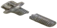
Actuators 14 00185 i002
CorrosionDamage caused by chemical reactions such as rust.Actuators 14 00185 i003
NotchesSmall dents or cuts caused by improper machines or external friction.
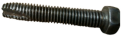
Actuators 14 00185 i004
DentsSmall and deep dents on surface of bolt, typically circular or elliptical in shape.
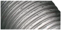
Actuators 14 00185 i005
ScratchesLong and shallow linear marks caused by external friction.Actuators 14 00185 i006
Table 3. Main performance parameters of the model.
ParametersPeak RAMSizeTotal SamplesAverage Inference TimeTrue PositivesFalse NegativeFalse Negative Rate
2.71 M10.33 MB5.5 MB800.049 s7911.25%
Table 4. Camera (left and right) calibration parameter results.
NameCamera MatrixDistortion CoefficientsRectification MatrixProjection Matrix
Camera
(left)
442.8 0 441.7 0 443.9 236.94 0 0 1 0.0417 0.0257 0.0003 0.0095 0 0.9823 0.0052 0.1874 0.0036 1 0.0086 0.1874 0.0077 0.9823 529.3 0 623.6 0 0 529.3 231.6 0 0 0 1 0
Camera
(right)
427.8 0 438.9 0 429.7 229.9 0 0 1 0.0309 0.0170 0.0014 0.0060 0 0.9818 0.0020 0.1899 0.0036 1 0.0079 0.1898 0.0084 0.9818 529.3 0 623.6 27.6 0 529.3 231.6 0 0 0 1 0
Table 5. Average and maximum relative errors of size measurement under different lighting conditions. (The gray value ranges from 0 to 255, with 255 representing the maximum.)
GroupGray ValueAverage Relative Error (%)Maximum Relative Error (%)
101.14
2500.662.2
31000.481.4
41500.631.7
52000.641.3
62550.411
Disclaimer/Publisher’s Note: The statements, opinions and data contained in all publications are solely those of the individual author(s) and contributor(s) and not of MDPI and/or the editor(s). MDPI and/or the editor(s) disclaim responsibility for any injury to people or property resulting from any ideas, methods, instructions or products referred to in the content.

