Snake Robot Gait Design for Climbing Eccentric Variable-Diameter Obstacles on High-Voltage Power Lines

Abstract

This paper presents a novel gait design for serpentine robots to smoothly wrap around and traverse vibration-damping hammers along overhead power lines. Cubic quasi-uniform B-spline curves are utilized to seamlessly transition between helical segments of varying diameters during obstacle crossing, effectively reducing motion-induced impacts. The design begins by determining the control points of the B-spline curves to ensure posture continuity and prevent collisions with surrounding hardware obstacles, resulting in the derivation of an obstacle-crossing curve equation. Using this equation, the node coordinates and postures of individual robot units are computed, followed by the calculation of joint angles via inverse kinematics. A dual-chain Hopf oscillator is then employed to generate the obstacle-crossing gait. The feasibility of the proposed gait is validated through simulations in CoppeliaSim and Simulink, which model the robot’s motion as it wraps around and crosses eccentric obstacles with varying diameters. Additionally, a simulation platform is developed to analyze variations in joint angles and angular velocities during obstacle traversal. Results demonstrate that the gait, generated by combining cubic quasi-uniform B-spline curves with a dual-chain Hopf oscillator, achieves smooth and stable wrapping and crossing of vibration-damping hammers. The robot exhibits no abrupt changes in joint angles, smooth angular velocity profiles without sharp peaks, and impact-free joint interactions, ensuring reliable performance in complex environments.

1. Introduction

Regular inspection of overhead power transmission cables is crucial for ensuring the efficient delivery of electricity to users and for the early detection and maintenance of faults. Traditional inspection robots for overhead power lines typically have two or three rigid arms, making them bulky and heavy, which leads to low inspection efficiency [1]. The serpentine robot, with its high redundancy and environmental adaptability, has become an ideal choice for inspecting overhead power lines. However, obstacles such as vibration-damping hammers (a common component in high-voltage transmission lines), suspension clamps, and splice tubes on the transmission lines pose challenges to the robot’s obstacle-crossing capability and motion control. During obstacle traversal, the key challenge is to avoid collisions between the robot’s body and the cables or hardware components, while ensuring smooth traversal. This is critical for ensuring the safe and reliable operation of the serpentine robot along the overhead power lines.

In recent years, scholars worldwide have extensively researched the climbing and obstacle-crossing capabilities of serpentine robots. Tatsuya et al. [2,3] proposed defining the irregular spiral shape formed by the serpentine robot as a combination of axis, cross-section, and pitch angles, allowing better adaptation to pipes with continuously varying and non-circular cross-sections. Furthermore, the team enabled the robot’s climbing motion by combining displacement control with suspension movement, which allowed the serpentine robot to climb ladders. Qi Wei et al. [4] introduced the use of hyperbolic functions to generate helical wave curves, enabling the serpentine robot to traverse branched pipelines. Wang Wei et al. [5] proposed an obstacle-crossing method in which the serpentine robot’s head grasps obstacles, enabling it to cross various line fittings. Jingwen Lu et al. [6] introduced an S-shaped rolling gait based on curve transformation design to enhance the robot’s ability to cross branched pipelines. Huizhuo Yang et al. [7] proposed an adaptive climbing method based on compliant control, allowing the serpentine robot to climb curved pipelines. Zhipeng Li et al. [8] applied reinforcement learning to enable the robot to cross two parallel rods, with the designed controller facilitating faster swinging to the target height. Yuta Iguchi et al. [9] developed a serpentine robot with mobile joints and designed an obstacle-crossing controller, enabling the robot to climb stairs. Sheraz Yaqub et al. [10] proposed a helical gait to address diameter discontinuities, allowing the serpentine robot to cross obstacles with diameter variations on both vertical and horizontal pipelines.

Most previous studies on serpentine robot obstacle crossing focus on gradual or sudden diameter changes of cylindrical obstacles, where the obstacle axis aligns with the pipeline or cable axis. Research on cases where there is an offset between the axes is relatively limited. This paper uses the case of the serpentine robot wrapping around and crossing vibration dampers on overhead power lines to explore methods for generating obstacle-crossing gaits for eccentric, diameter-varying obstacles.

Different obstacle-crossing gaits necessitate the use of specialized gait generation controllers. Koki Harada et al. [11] designed a controller for the serpentine robot to slide on smooth surfaces based on a dynamic model. Mizuki Nakajima et al. [12] developed a motion controller capable of tracking the serpentine robot’s trajectory along multiple slopes, though it is not suitable for cable climbing. Xupeng Liu et al. [13] proposed a CPG network model based on an improved Hopf oscillator design, enabling the serpentine robot to perform gaits such as creeping, traveling wave, lateral winding, arc rolling, and spiral rolling, with smooth transitions between gaits. They also addressed inconsistent waveform amplitudes using decoupled bifurcation parameters. Xuan Liu et al. [14] developed a reinforcement learning-based target tracking controller, enabling the serpentine robot to generate natural and smooth movement patterns. When a joint actuator fails, Ryo Ariizumi et al. [15] proposed a controller that can still track the originally set path. Yongdong Wang et al. [16] applied a sine curve control method and a hybrid force–position controller to improve the serpentine robot’s stability in congested pipelines. However, when the robot’s joints fail to follow the target angles, it may cause the motors to reset. Guifang Qiao et al. [17] developed a motion controller based on a three-layer central pattern generator (CPG), enabling continuous and smooth three-dimensional motion control for the serpentine robot. The above gait generation controllers provide the serpentine robot with diverse motion capabilities, each with its own advantages and disadvantages. They should be selected flexibly based on specific requirements. Since the yaw and roll joints of each segment of the serpentine robot must move simultaneously during obstacle crossing, this paper uses a dual-chain Hopf oscillator to decouple the movement of these joints and control the robot’s obstacle-crossing gait.

In summary, to enable the serpentine robot to coil and cross obstacles such as vibration dampers on overhead transmission lines, this paper models the vibration damper as an obstacle with an eccentric offset from the cable. The robot’s obstacle-crossing gait is planned using a kinematic model and cubic quasi-uniform B-spline curves to smooth the transition between two segments of eccentric, varying-diameter helical lines. The obstacle-crossing curve is generated by connecting the two segments, with B-spline control points defined to ensure a smooth connection. The robot’s joint angles, initial values, and maximum values during the obstacle-crossing movement are calculated using the obstacle-crossing posture curve equation, which is then input into the dual-chain Hopf oscillator to generate control signals for the yaw and roll joints. Finally, simulation and prototype experiments of the robot’s obstacle-crossing process over eccentric, varying-diameter obstacles are conducted to verify the feasibility of the obstacle-crossing gait.

2. Structure of Snake Robot Modules and Operational Conditions

This paper uses a serpentine robot composed of P-R-S units as the experimental subject. Figure 1 shows the robot’s operating environment, and Figure 2 illustrates the unit structure. Each unit consists of a yaw joint component, a roll joint component, and a translational joint component. These components are mechanically coupled via customized connectors to inner sleeves. Specifically, the yaw and roll joint components enable adjacent module articulation in pitch and rotational motions respectively through embedded servomotors. The translation joint component utilizes threaded fasteners to secure the fork part to the scale sleeve, where reciprocating of the translational servomotor within constrained angular ranges drives periodic axial displacement of the scale sleeve. Eight rollers are strategically arranged between the inner sleeves and scale sleeve to facilitate relative sliding motion. The roll joint incorporates servo horn connectors at its distal end, establishing mechanical linkages between adjacent robotic units through servo horn couplings that interconnect roll and yaw joints across neighboring modules.

On high-voltage transmission lines, the serpentine robot mainly moves in two ways: crawling mode and spiral wrapping mode. Figure 3a illustrates the crawling mode of the robot’s forward movement [18]. The robot, helically wrapped around the high-voltage power transmission line with constant pitch, achieves advancement along a constant-pitch helical trajectory through the translational module that actuates the scale sleeves of the odd-numbered and even-numbered units in an alternating manner. The unique structure of the scale sleeves anisotropic friction, with lower friction in the forward direction and higher friction in the reverse, enabling the robot to traverse rough surfaces. Figure 3b illustrates the robot’s movement in spiral wrapping mode, where the serpentine robot is divided into the head, middle, and tail segments. Initially, the serpentine robot wraps around the high-voltage transmission line in an evenly spaced spiral. During movement, the robot’s tail tightly wraps around the transmission line first. Then, using the tail as a pivot, the head and middle body stretch forward. The head then tightly wraps around the line, and finally, by retracting the body and tail, the robot moves forward.

Based on the installation method of the vibration damper, the section of the line with the damper is simplified. Under fully tensioned conditions, the flexible deformation of the cable is negligible, and it can thus be modeled as a rigid structure. Dynamic oscillation of the line during motion are also neglected in this analysis. As shown in Figure 4, the vibration damper is simplified as an eccentric variable-diameter obstacle on the cable. The cable is simplified as a cylinder with radius r₁, and the vibration damper as a cylinder with radius r₂. The axes of these two cylinders differ by (r₂ − r₁) along the Y-axis. Figure 5 shows the positional relationship between the cable and the obstacle in the XOY plane, where OA and OB represent the centers of the cable and the eccentric variable-diameter obstacle in the XOY plane, respectively.

This study on the gait of the snake-like robot crossing the vibration damper is divided into two parts: (1) proposing a motion gait that enables the robot to move along the cable and overcome eccentric variable-diameter obstacles while avoiding collisions with the obstacle; and (2) analyzing whether singular configurations exist during the robot’s movement under this gait, to prevent abrupt or discontinuous changes in joint angular velocity.

3. Mathematical Model of Snake Robot Obstacle Crossing

3.1. Kinematic Model

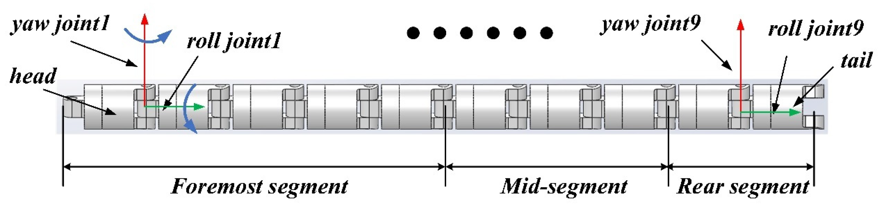
For convenience, the joints of the snake-like robot are numbered such that the unit with the roll joint not connected to other units is labeled as Joint 1. The remaining joints are numbered sequentially based on their distance from Joint 1. The robot is divided into three sections: Sections 1 to 5 as the head, Sections 6 to 8 as the middle, and Sections 9 to 10 as the tail, as shown in Figure 6. The robot’s dimensional parameters are listed in

Table 1. Dimensions of snake robot.

Parameter	Value
number of joints	10
joint length	105 mm
joint diameter	63 mm
degrees of freedom per joint	2

, where the joint length is defined as the distance from the steering gear connector to the center of the steering gear disc in the deflection joint.

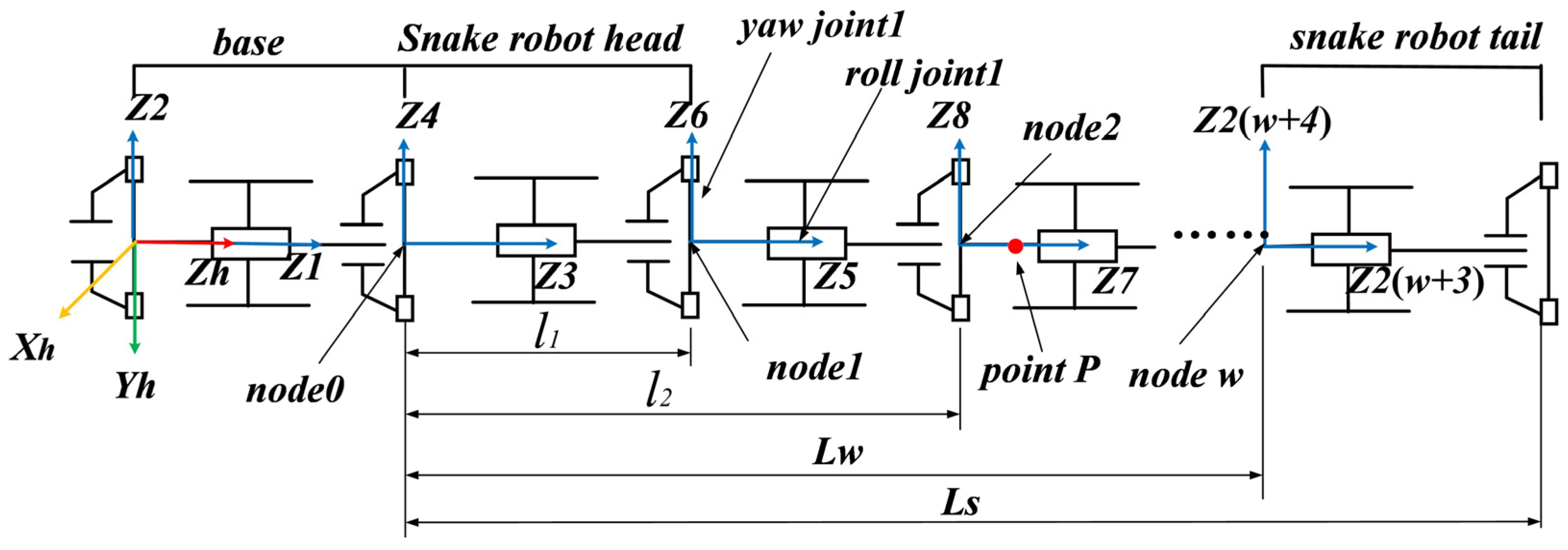
As a multi-degree-of-freedom robot, each joint angle change of the snake-like robot alters its spatial posture. To accurately describe the mapping between the spatial positions of points on the robot and the joint angles, a coordinate system is established at each joint. The D-H parameter method is used to build the robot’s kinematic model. For convenience in processing the calculation results, a virtual unit is added in front of the robot’s head as the base, as shown in Figure 7. Here, the coordinate system {h} serves as the reference frame. Odd-numbered coordinate systems denote revolute joint frames, while even-numbered ones represent deflection joint frames.

The junction between two units is a node. Taking the robot’s head as the reference, the position of node w is L_w:

$$L_w=w{\displaystyle \frac{L_s}{N_s}}$$

(1)

In this case, N_s represents the total number of units in the snake robot’s body, and L_s denotes the total length of the robot.

To describe the relationship between the spatial position of each point on the snake robot and the angles of its joints, an improved DH method is used to establish the roll transformation matrix, where j = 1, 3, 5, 7…, and α_i represents the angle of the i joint:

$$\left\{\begin{array}{c}{}_1{}^{h}R=\left[\begin{array}{ccc}cos {\alpha }_i& -sin {\alpha }_i& 0\\ sin {\alpha }_i& cos {\alpha }_i& 0\\ 0& 0& 1\end{array}\right]\\ {}_{j+1}{}^{j}R=\left[\begin{array}{ccc}cos {\alpha }_i& -sin {\alpha }_i& 0\\ 0& 0& -1\\ sin {\alpha }_i& cos {\alpha }_i& 0\end{array}\right]\\ {}_{j+2}{}^{j+1}R=\left[\begin{array}{ccc}cos {\alpha }_i& -sin {\alpha }_i& 0\\ 0& 0& 1\\ -sin {\alpha }_i& -cos {\alpha }_i& 0\end{array}\right]\end{array}\right.$$

(2)

The coordinate transformation formula for any point p on the snake robot between the joint coordinate system i and the reference coordinate system (coordinate system h) is as follows:

$$p^h={}_i{}^{h}R\times p^i$$

(3)

When pⁱ = (0 1 0)^T (where i is an even number), the calculated p^h represents the posture of the corresponding unit of the snake robot relative to the reference coordinate system.

3.2. Obstacle-Crossing Gait Planning

There are two phases for the snake robot to cross an eccentric large-diameter obstacle: first, the robot climbs from the cable to the eccentric large-diameter obstacle; second, it returns from the obstacle back to the cable.

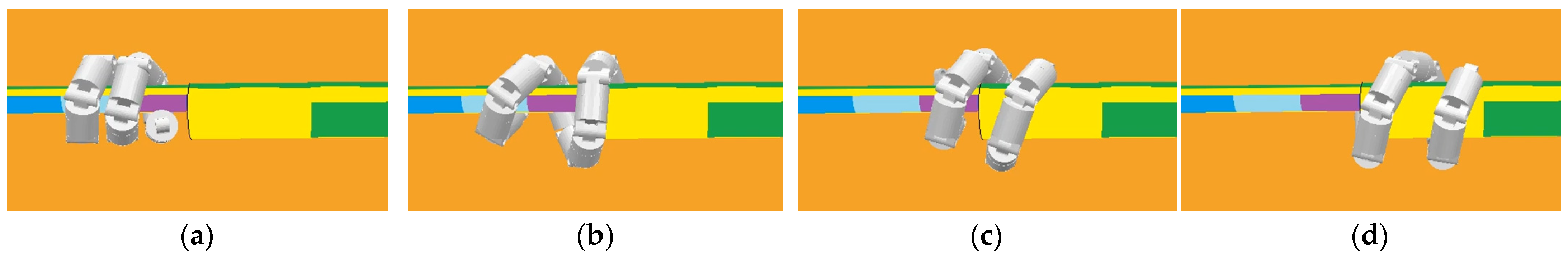
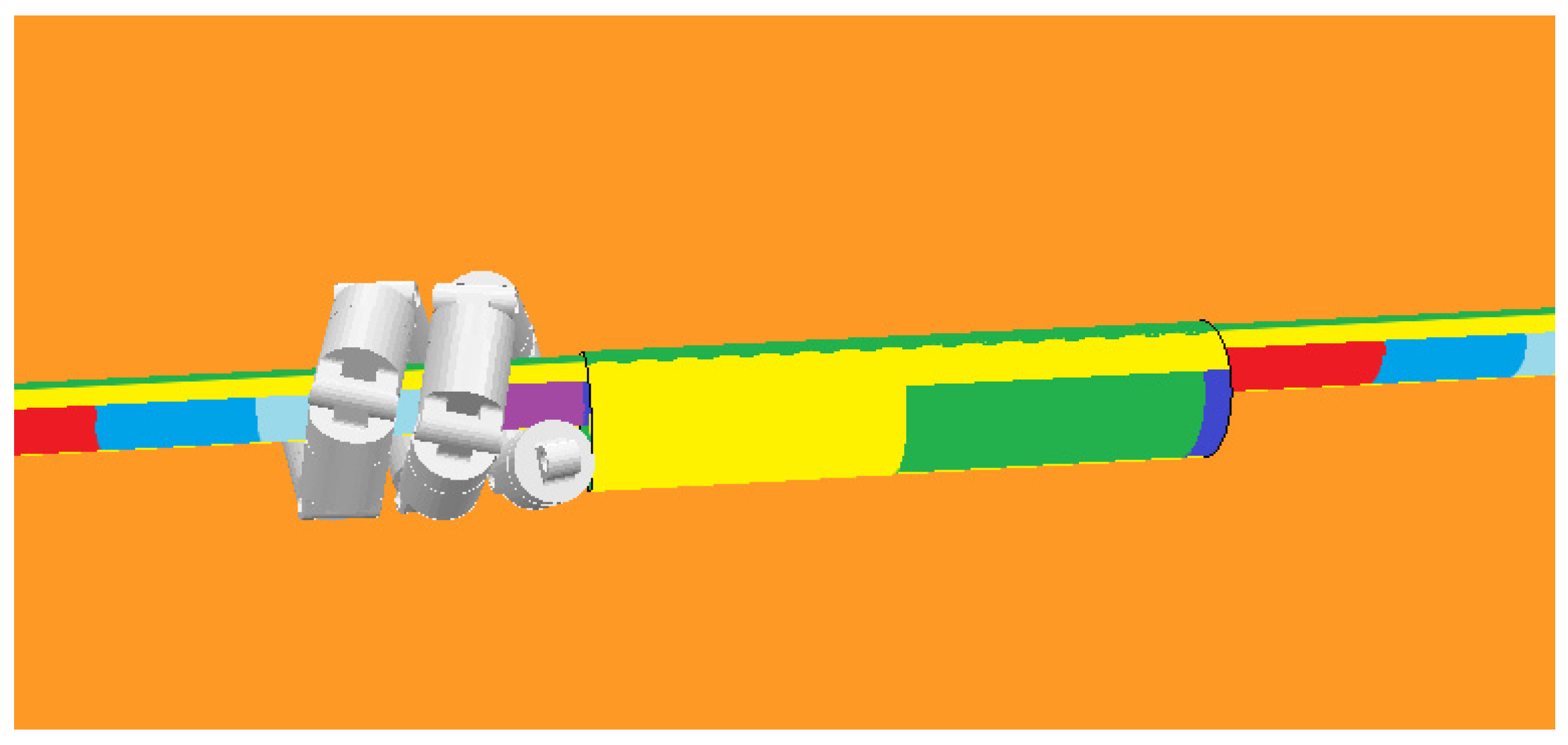
Figure 8 illustrates the posture changes of the snake robot as it climbs from the cable onto the eccentric large-diameter obstacle. First, the robot spirals around the cable in a helical posture (Figure 8a); next, it elongates its body with the tail segment as the base, then spirals the head segment around the obstacle (Figure 8b); then, continuing with the tail as the base, the robot extends the body further, bringing the middle segment onto the obstacle and spiraling it around the obstacle (Figure 8c); finally, the robot elongates its body to move forward and pulls the tail segment onto the obstacle (Figure 8d).

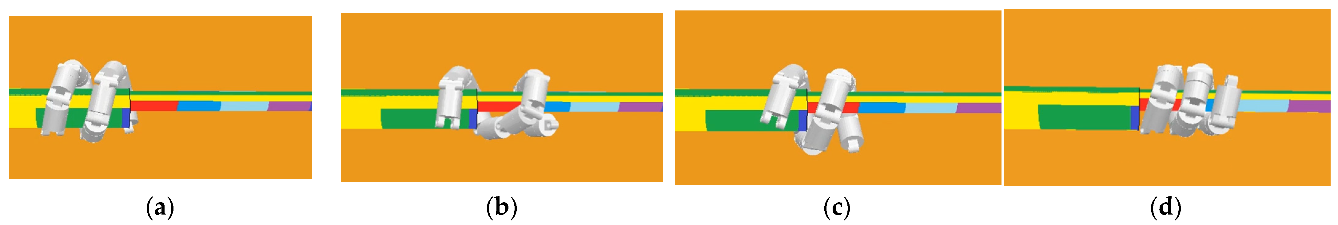
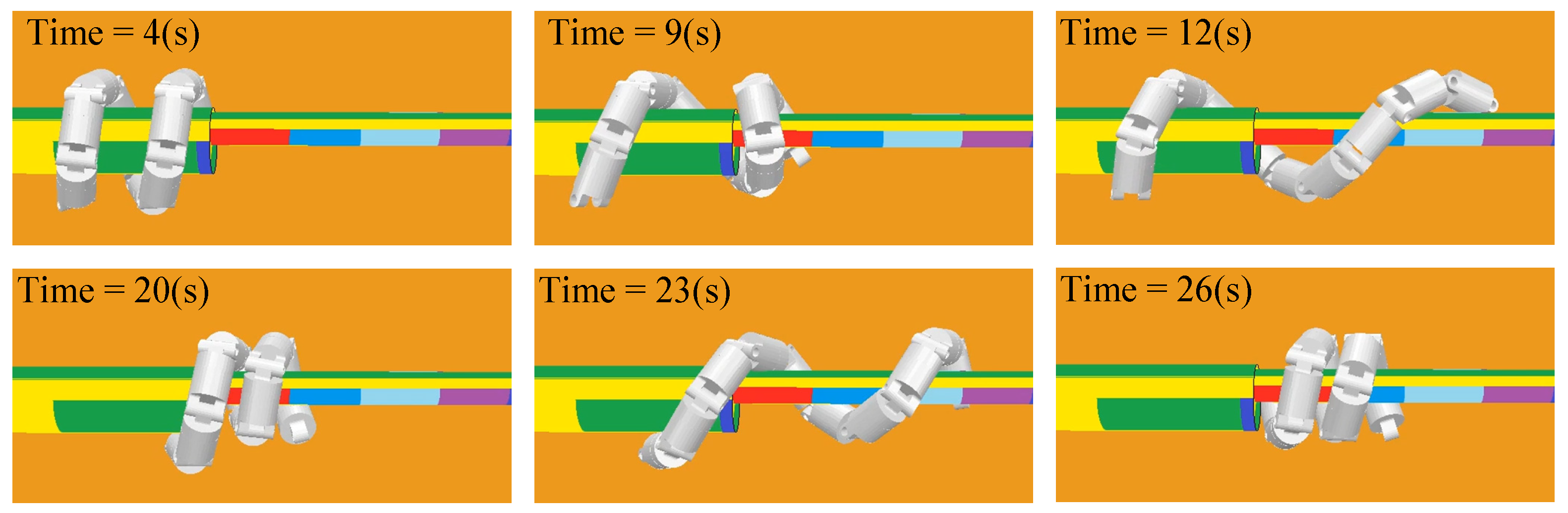
Figure 9 illustrates the posture changes of the snake robot as it moves from the eccentric large-diameter obstacle back to the cable. The process is similar to that in Figure 8, but reversed. Therefore, this paper provides a detailed analysis of the process in which the robot climbs from the cable onto the eccentric large-diameter obstacle, and later conducts simulations and experimental analysis of both processes.

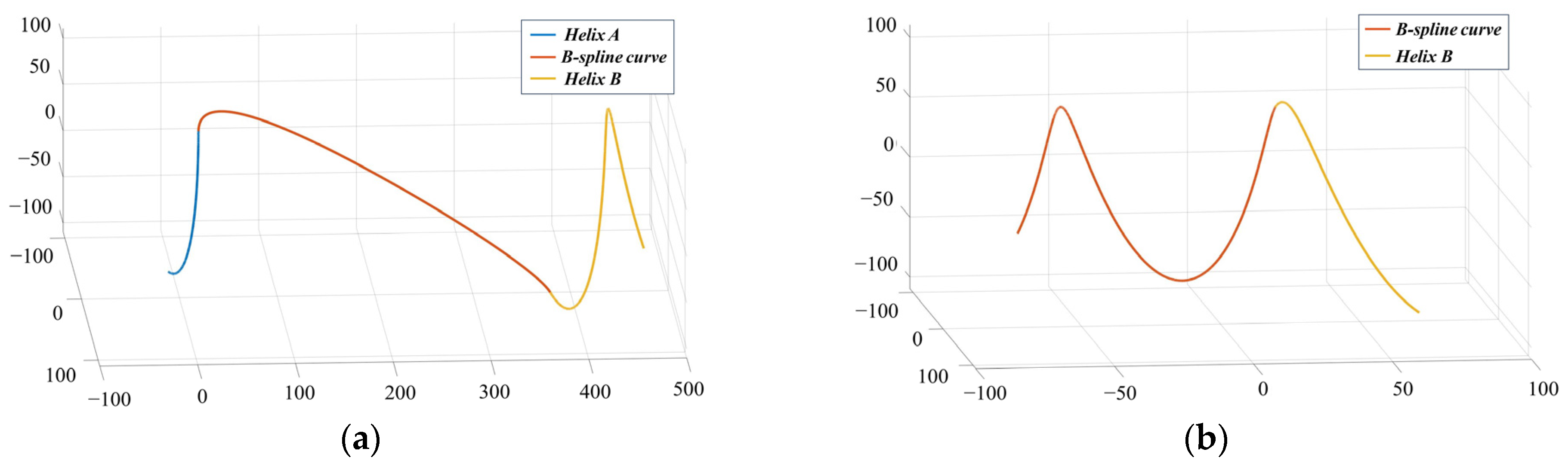
For the case of the snake robot climbing from the cable onto an eccentric large-diameter obstacle, the robot’s posture curve during the obstacle traversal is first derived. Then, by examining the correspondence between the obstacle traversal posture curve and the robot’s joint positions, the joint angles of the robot are calculated. During the obstacle traversal, the snake robot follows two segments of spirals with different diameters. To avoid internal constraint forces during the robot’s motion, a transition curve is added between the two spiral segments to smoothly connect them. The posture curves of the snake robot in Figure 8a,d represent equidistant spirals; the posture in Figure 8b corresponds to the posture curve shown in Figure 10a, while the posture in Figure 8c corresponds to the curve in Figure 10b.

In Figure 10a, the posture curve of the snake robot consists of Helix A (representing the robot’s tail segment), a transition curve (representing the robot’s middle segment), and Helix B (representing the robot’s head segment). In Figure 10b, the posture curve of the snake robot is made up of Helix B (representing the middle and head segments of the robot) and the transition curve (representing the robot’s tail segment).

The equations of the curves for Helix A and Helix B are as follows:

$$C_A\left(q_A\right)=\left\{\begin{array}{c}{x}_A=r_A{cos q}_A\\ y_A=r_A{sin q}_A\\ z_A={\displaystyle \frac{h_A}{2\pi }}{q}_A\\ {\theta }_A=2\pi T_{sA}\\ h_A={\displaystyle \frac{\sqrt{{L_s}^2-{\left(r_A{\ast \theta }_A\right)}^2}}{T_{sA}}}\\ r_A={\displaystyle \frac{r_t+r_s}{\cos \left(\frac{{\theta }_A}{2\ast N_s}\right)}}\end{array}\right.$$

(4)

$$C_B\left(q_B\right)=\left\{\begin{array}{c}{x}_B=r_B{cos q}_B\\ y_B=r_B{sin q}_B-(r_B-r_A)\\ z_B={\displaystyle \frac{h_B}{2\ast \pi }}\ast q_B+H_B\\ {\theta }_B=2\ast \pi \ast T_{sB}\\ h_B={\displaystyle \frac{\sqrt{{L_s}^2-{(r_B\ast {\theta }_B)}^2}}{T_{sB}}}\\ r_B={\displaystyle \frac{r_t+r_s}{\cos \left(\frac{{\theta }_B}{2\ast N_s}\right)}}\end{array}\right.$$

(5)

In this context, q_A and q_B are defined as the instantaneous angular parameters governing the motion of the serpentine robot along Helix A and Helix B, respectively; r_A and r_B represent the wrapping radii of Helix A and Helix B, respectively; r_s is the radius of the snake robot’s unit; r_t is the radius of the cable or obstacle; h_A and h_B denote the lead of Helix A and Helix B, respectively; H_B is the offset of Helix B along the Z-axis; T_sA and T_sB refer to the number of turns of Helix A and Helix B, which indicates the maximum number of turns the snake robot can make when the lead is h_A or h_B; L_s is the total length of the snake robot; N_s represents the total number of units in the snake robot’s body.

3.3. Transition Curve

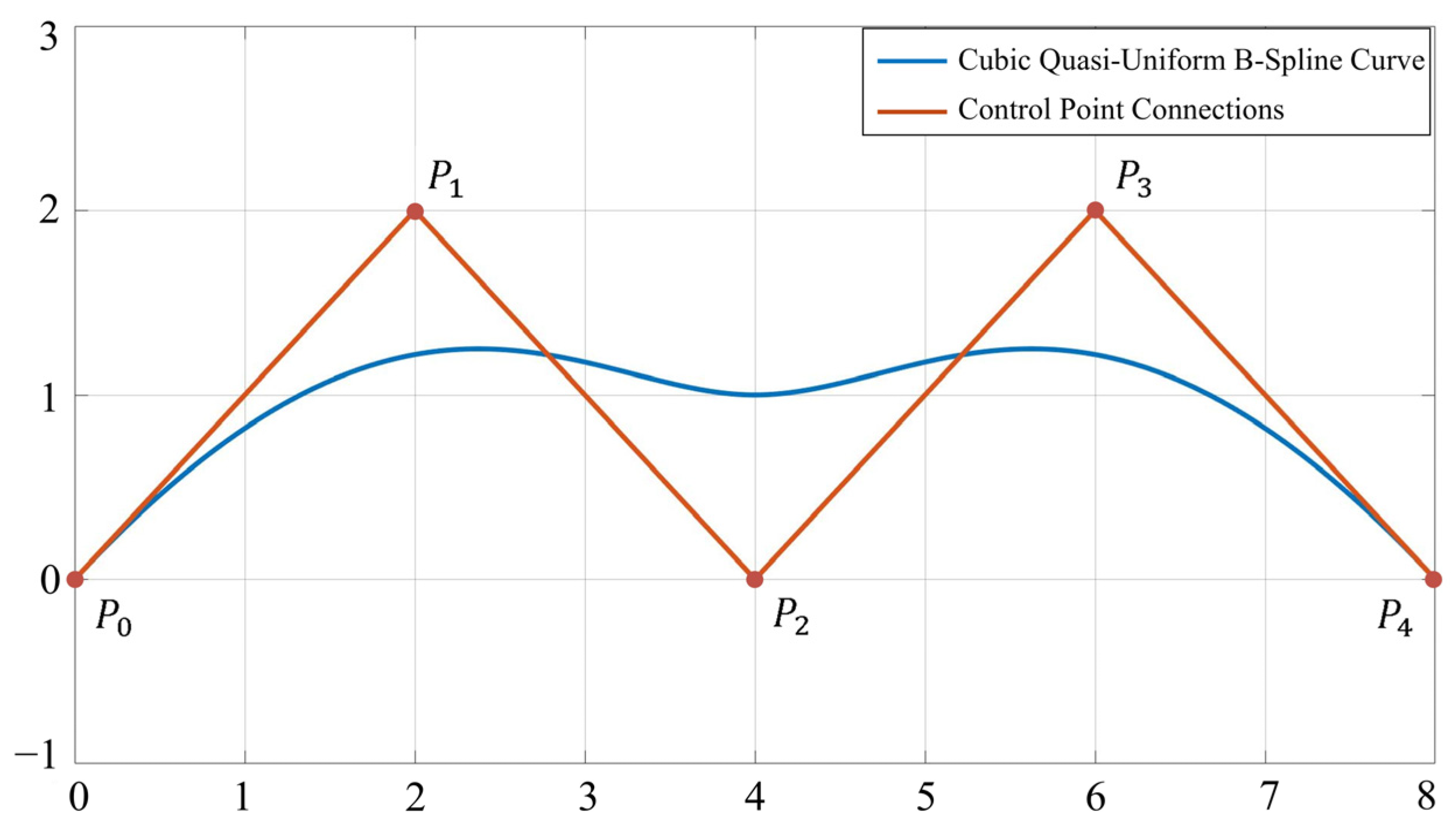
To ensure a smooth transition between the two helical segments, this study uses quasi-uniform B-spline curves for the smooth blending of the curves. The tangent directions at the endpoints of the quasi-uniform B-spline curve are aligned with the direction of the vectors formed by the last two endpoints. As shown in Figure 11, the tangent directions at points P₀ and P₄ of the B-spline curve align with the vectors $\overrightarrow{P_0{P}_1}$ and $\overrightarrow{P_0{P}_4}$, respectively. Therefore, by appropriately selecting the control points, we ensure that the left and right derivatives at the connection points between the helical curve and the quasi-uniform B-spline curve are equal, achieving a smooth transition between the two. Higher-order B-splines yield smoother curves. To ensure smooth blending between the curves, a cubic quasi-uniform B-spline curve is selected in this study.

The cubic quasi-uniform B-spline curve consists of five control points, P₀ to P₄, where P₀ is the point of intersection between the B-spline curve and Helix A, and P₄ is the intersection between the B-spline curve and Helix B. To determine the equation of the cubic quasi-uniform B-spline curve shown in Figure 10, the coordinates of the five control points, P₀ to P₄, must first be established. 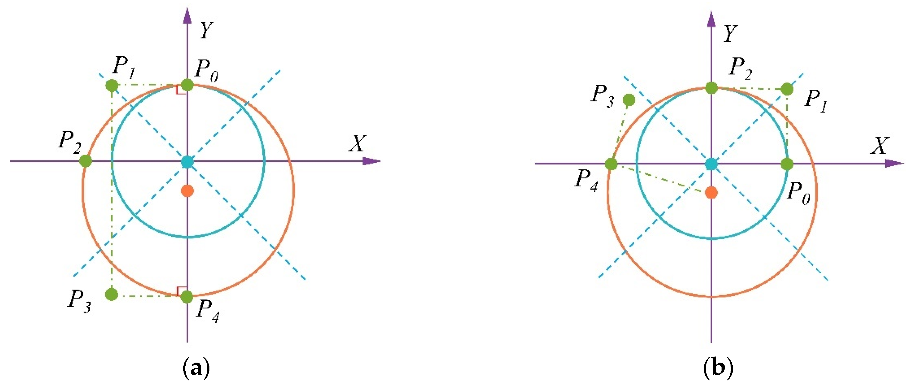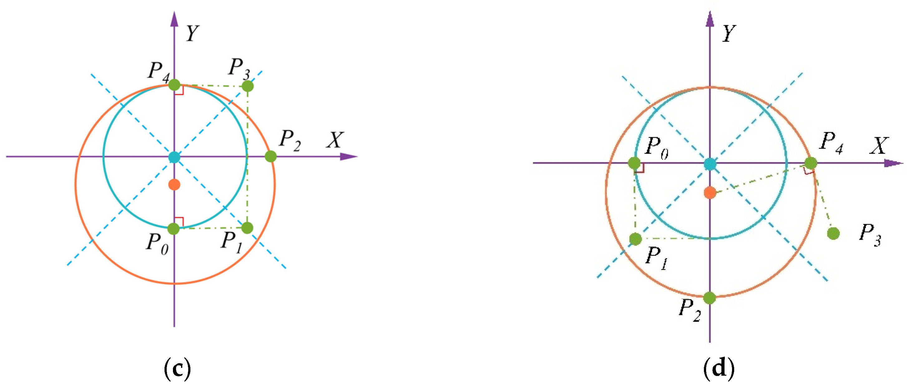Since the position of point P₀ can vary along the plane of intersection between the obstacle and the cable during the robot’s motion, four control point selection schemes are proposed in this study to reduce computational complexity, as illustrated in Figure 12.

Selection of point P₀: The point P₀ is placed on the coordinate axis, and the equation of the axis is solved simultaneously with Equation (4). The coordinates of point P₀ are given below, where k₁ represents the slope of the coordinate axis on which P₀ lies.

$$\left\{\begin{array}{c}{x}_{P0}={\displaystyle \frac{\pm r_A}{\sqrt{{k_1}^2+1}}}\\ {x_{P0}}^2+{y_{P0}}^2={r_A}^2\\ z_{P0}={\displaystyle \frac{h_A}{2\pi }}(\arccos ({\displaystyle \frac{x_{P0}}{r_A}}\left)\right)\end{array}\right.$$

(6)

Selection of point P₁: To ensure a smooth connection between the B-spline curve and Helix A, the tangent direction of Helix A at point P₀ must be the same as the tangent direction of the B-spline curve at P₀. The tangent direction of the B-spline curve at P₀ aligns with the vector $\overrightarrow{P_0{P}_1}$, and to avoid intersection with the cable, the projection length of vector $\overrightarrow{P_0{P}_1}$ on the XOY plane must equal the roll radius r_A of Helix A. The coordinate of point P₁ is given by Equation (7), where j is a scaling factor in the formula for controlling the geometric characteristics of a B-spline curve at the connection point P₀, ensuring a smooth transition between the curve and Helix A:

$$\left\{\begin{array}{c}{(x_{P1}-x_{P2})}^2+{(y_{P1}-y_{P2})}^2={r_A}^2\\ \left[\begin{array}{c}{x}_{P0}^{\prime }\\ y_{P0}^{\prime }\\ z_{P0}^{\prime }\end{array}\right]=j\left[\begin{array}{c}{x}_{P0}-x_{P1}\\ y_{P0}-y_{P1}\\ z_{P0}-z_{P1}\end{array}\right]\\ j>0\end{array}\right.$$

(7)

Selection of point P₂: In the XOY plane, point P₂ is the intersection of another coordinate axis and a circle with a radius of r_B. Here, L₁₃ represents the distance between points P₁ and P₃ along the Z-axis, which is calculated through Equation (13), and k₂ is the slope of the coordinate axis containing point P₂. The coordinate equation of point P₂ is given by:

$$\left\{\begin{array}{c}{x}_{P2}={\displaystyle \frac{k_2\left(r_B-r_A\right)\pm \sqrt{({k_2{r}_B)}^2-{r_A}^2+2r_B{r}_A}}{{k_2}^2+1}}\\ {x_{P2}}^2+{{(y}_{P2}-(r_B-r_A))}^2={r_B}^2\\ z_{P2}=z_{P1}+{\displaystyle \frac{L_{13}}{2}}\end{array}\right.$$

(8)

Equation (8) has two solutions, from which one is selected based on the rotation direction of Helix A.

Selection of P₃ point. The coordinates of P₃ need to be calculated based on the coordinates of P₄. Similarly, to ensure smooth connection between the B-spline curve and Helix B, the tangent direction of Helix B at P₄ must align with the tangent direction of the B-spline curve at P₄. The tangent direction of the B-spline curve at P₄ coincides with the direction of vector $\overrightarrow{P_3{P}_4}$, and the projection length of vector $\overrightarrow{P_3{P}_4}$ in the XOY plane equals the rotation radius r_A of Helix A. Based on this, the coordinates of P₃ in the XOY plane can be determined as follows:

$$\left\{\begin{array}{c}{(x_{P4}-x_{P3})}^2+{(y_{P4}-y_{P3})}^2={r_A}^2\\ \left[\begin{array}{c}{x}_{P4}^{\prime }\\ y_{P4}^{\prime }\\ z_{P4}^{\prime }\end{array}\right]=j\left[\begin{array}{c}{x}_{P3}-x_{P4}\\ y_{P3}-y_{P4}\\ z_{P3}-z_{P4}\end{array}\right]\\ z_{P3}=z_{P2}+{\displaystyle \frac{L_{13}}{2}}\\ j>0\end{array}\right.$$

(9)

Selection of P₄ point. To ensure that the snake robot does not slip off the cable, in the XOY plane, P₄ is set at the intersection of the coordinate axis and the circle with radius r_B. This axis is the same as the one where P₀ lies. The coordinate equation for P₄ is as follows:

$$\left\{\begin{array}{c}{x}_{P4}={\displaystyle \frac{k_1\left(r_B-r_A\right)\pm \sqrt{({k_1\ast r_B)}^2-{r_A}^2+2\ast r_B\ast r_A}}{{k_1}^2+1}}\\ {x_{P4}}^2+{{(y}_{P4}-(r_B-r_A))}^2={r_B}^2\\ z_{P4}={\displaystyle \frac{h_B}{2\ast \pi }}\left(\arccos \left({\displaystyle \frac{x_{P4}}{r_B}}\right)\right)+H_B\end{array}\right.$$

(10)

Equation (10) has two solutions, and one is selected based on the rotation direction of Helix A.

Based on the selected five control points, the cubic quasi-uniform B-spline curve is computed, with the knot vector U = {0, 0, 0, 0, 0.5, 1, 1, 1, 1}. The resulting cubic quasi-uniform B-spline curve function is expressed as follows. p_i represents the control points of the B-spline curve; u is a continuous parameter variable defined over the range specified by the knot vector U, which parameterizes points along the curve; and $B_{i,3}\left(u\right)$ denotes the basis functions of the B-spline curve:

$$p(u)=\sum _{i=0}^4{p}_i\times B_{i,3}\left(u\right)$$

(11)

equivalent to

$$p(u)=\left[\begin{array}{c}{x}_p\left(u\right)\\ y_p\left(u\right)\\ z_p\left(u\right)\end{array}\right]$$

(12)

The appropriate control point scheme is selected based on the position of the connection point between the middle and tail segments of the snake robot. The pre-obstacle crossing posture of the snake robot is shown in Figure 8a. The position of the connection point between the middle and tail segments of the robot is closest to the positive half-axis of the Y-axis, so the coordinates of the control point follow the scheme in Figure 12a. Based on this, the cubic quasi-uniform B-spline curve is calculated and combined with the helix to obtain the obstacle crossing posture curve of the snake robot shown in Figure 8b.

3.4. Obstacle-Crossing Posture Curve of the Snake-like Robot

Since the length of the cubic quasi-uniform B-spline curve is equal to the length of the middle segment of the snake robot, the following equation can be written, where l_link is the length of a snake robot unit, namely the joint length in Table 1, to solve for the parameter L₁₃:

$${\int }_0^1\sqrt{{\left({x_p\left(u\right)}^{\prime }\right)}^2+{\left({y_p\left(u\right)}^{\prime }\right)}^2+{\left({z_p\left(u\right)}^{\prime }\right)}^2}du=3l_{link}$$

(13)

Substitute the obtained L₁₃ into Equations (9) and (10), to solve for the parameter H_B in Helix B. By solving Equations (4), (5) and (12) simultaneously, the posture curve function in Figure 10a is obtained as:

$$\left\{\begin{array}{c}x=r_A\times {cos q}_A+r_B\times {cos q}_B+x_p\left(u\right)\\ y=r_A\times {sin q}_A+r_B\times {sin q}_B-(r_B-r_A)+y_p\left(u\right)\\ x={\displaystyle \frac{h_A}{2\pi }}{q}_A+{\displaystyle \frac{h_B}{2\pi }}{q}_B+H_B+z_p\left(u\right)\end{array}\right.$$

(14)

where the range of q_A is $q_A\in \left[\begin{array}{cc}arctan k_1-2\times T_{sA}\times \pi /5& arctan k_1\end{array}\right]$\ and the range of q_B is $q_B\in \left[\begin{array}{cc}\arccos \left(x_{p4}/r_B\right)& \arccos \left(x_{p4}/r_B\right)+T_{sB}\times \pi \end{array}\right]$.

To solve for the posture curve of the snake robot shown in Figure 8c, the selection rule for the control points is the same as in the first case, and the calculation methods for parameters L₁₃ and H_B are the same as in the first case. Thus, the posture curve function in the second case is given by:

$$\left\{\begin{array}{c}x=r_B\times {cos q}_B+x_p\left(u\right)\\ y=r_B\times {sin q}_B-(r_B-r_A)+y_p\left(u\right)\\ x={\displaystyle \frac{h_B}{2\pi }}{q}_B+H_B+z_p(u)\\ \arccos \left({\displaystyle \frac{x_{P4}}{r_B}}\right)\le q_B\le \arccos \left({\displaystyle \frac{x_{P4}}{r_B}}\right)+{\displaystyle \frac{8\times T_{sB}\times \mathsf{\pi }}{5}}\end{array}\right.$$

(15)

4. Robot Obstacle-Crossing Gait Generation

4.1. Calculation of Joint Angles for the Snake Robot

To calculate the joint angles of the snake robot corresponding to the posture curve shown in Figure 10a, first, the coordinates of the nodes between the robot’s units are determined based on the posture curve; then, the gradient at each node is calculated based on the node coordinates, which represents the posture of the robot’s unit at the node; finally, these values are substituted into the kinematic model to compute the joint angles of the snake robot.

Step 1: To facilitate the processing of the calculation results, two additional units are added to the snake robot as a base, as shown in Figure 7. The angle of the helical curve corresponding to node w in the first section of the snake robot is:

$$q_w=T_{sB}\times 2\times \mathsf{\pi }\times L_s/L_w$$

(16)

where w is a positive integer with w ≤ 6. The corresponding q_w is substituted into the equation of Helix B to solve for the node’s position:

$$C_w=\left[\begin{array}{c}{x}_w\left(q_w\right)\\ y_w\left(q_w\right)\\ z_w\left(q_w\right)\end{array}\right]=\left[\begin{array}{c}{r}_B{cos q}_w\\ r_B{sin q}_w-(r_B-r_A)\\ {\displaystyle \frac{h_B}{2\pi }}{q}_w+H_B\end{array}\right]$$

(17)

Step 2: According to Equation (13), the length of the B-spline curve is the same as that of the snake robot’s middle segment. Therefore, the position of node w in the middle segment of the snake robot is given as follows, where w is a positive integer with 6 < w ≤ 9.

$$C_w=\left[\begin{array}{c}{x}_w\left(u\right)\\ y_w\left(u\right)\\ z_w\left(u\right)\end{array}\right]=\left[\begin{array}{c}{x}_p\left({\displaystyle \frac{w-6}{3}}\right)\\ y_p\left({\displaystyle \frac{w-6}{3}}\right)\\ z_p\left({\displaystyle \frac{w-6}{3}}\right)\end{array}\right]$$

(18)

Step 3: The tail segment of the snake robot corresponds to Helix A, and the calculation of the node positions is similar to Step 1. The position of node w is obtained as follows, where w is a positive integer with 9 < w ≤ 11.

$$C_w=\left[\begin{array}{c}{x}_w\left(u\right)\\ y_w\left(u\right)\\ z_w\left(u\right)\end{array}\right]=\left[\begin{array}{c}{r}_A{cos q}_w\\ r_A{sin q}_w\\ {\displaystyle \frac{h_A}{2\pi }}{q}_w\end{array}\right]$$

(19)

Step 4: Solve the gradient at each node, which also represents the posture of the snake robot unit at that node. For the nodes of the head and tail segments, Δq is a small angular increment, and the postures of the head and tail segments of the snake robot are:

$$G_w=\left[\begin{array}{c}{\displaystyle \frac{x_w\left(q_w+∆q\right)-x_w\left(q_w\right)}{∆q}}\\ {\displaystyle \frac{y_w\left(q_w+∆q\right)-y_w\left(q_w\right)}{∆q}}\\ {\displaystyle \frac{z_w\left(q_w+∆q\right)-z_w\left(q_w\right)}{∆q}}\end{array}\right]$$

(20)

For the middle segment of the snake robot, Δu is a small increment, and the posture of the middle segment of the snake robot is:

$$G_w=\left[\begin{array}{c}{\displaystyle \frac{x_w\left(u+∆u\right)-x_w\left(u\right)}{∆u}}\\ {\displaystyle \frac{y_w\left(u+∆u\right)-y_w\left(u\right)}{∆u}}\\ {\displaystyle \frac{z_w\left(u+∆u\right)-z_w\left(u\right)}{∆u}}\end{array}\right]$$

(21)

Step 5: Calculate the joint angles of the snake robot. The calculated G_w is substituted into the Equation system (22), where f is the coefficient.

$$\left\{\begin{array}{c}{G}_w=f\times {}_i{}^{h}R\times p^i \\ f>0 \\ i=2\times w+2\\ p^i={\left(\begin{array}{ccc}0& 1& 0\end{array} \right)}^T\end{array}\right.$$

(22)

Solve the system of equations to obtain the joint angles of the snake robot corresponding to the posture curve in Figure 10a. Similarly, the joint angles corresponding to the posture curve in Figure 10b can be obtained.

4.2. Mathematical Model of the Dual-Chain Hopf Oscillator

To achieve obstacle-crossing control for the snake robot, this paper selects the Hopf oscillator as the gait controller to generate the obstacle-crossing gait. However, a single Hopf oscillator cannot produce the desired obstacle-crossing gait, and thus the original oscillator model needs to be improved. The improved oscillator model is:

$$\left[\begin{array}{c}\dot{u}\\ \dot{v}\end{array}\right]=\left[\begin{array}{c}\mu (\rho -\left(u^2+v^2\right))u-kv\omega \\ \mu \left(\rho -\left(u^2+v^2\right)\right)v+ku\omega \end{array}\right]+\left[\begin{array}{c}{p}_u\\ p_v\end{array}\right]$$

(23)

$$k=\left\{\begin{array}{cc}0& when the timer is active\\ 1& when the timer is inactive\end{array}\right.$$

(24)

equivalent to

$$\dot{x}=f\left(x,\mu ,\rho ,\omega ,k\right)=F\left(x\right), x={\left(\begin{array}{cc}u& v\end{array}\right)}^T$$

(25)

where k is the oscillator enable parameter, and its value is changed through a timer to control the pause of the oscillator. The control logic is as follows: when the output value v of the oscillator meets the trigger condition of the timer, the timer starts counting, k = 0, and the oscillator pauses. When the timer reaches t_s (the pause time of the oscillator), the timer stops, is reset, and k = 1, allowing the oscillator to resume oscillating. The control flow is shown in Figure 13.

The snake robot studied in this paper consists of unit joints, with each unit containing two joints. Based on this structure, a Hopf oscillator with a double-chain configuration is selected, as shown in Figure 14.

The equation for the left chain in the double-chain model is:

$$\left\{\begin{array}{c}{\dot{x}}_{\mathrm{L}i}=\mathrm{F}\left(x_{\mathrm{L}i}\right)-\mathsf{\gamma }{b}_{\mathrm{L}i}\left(x_{\mathrm{L}i}-T_{\mathrm{L}i}^{-1}{x}_{\mathrm{L}i+1}\right)-h\left(x_{\mathrm{R}i}\right), i=1\\ \begin{array}{c}{\dot{x}}_{\mathrm{L}i}=\mathrm{F}\left(x_{\mathrm{L}i}\right)-\mathsf{\gamma }{a}_{\mathrm{L}i-1}\left(x_{\mathrm{L}i}-T_{\mathrm{L}i-1}{x}_{\mathrm{L}i-1}\right)-h\left(x_{\mathrm{R}i}\right), i=n\\ {\dot{x}}_{\mathrm{L}i}=\mathrm{F}\left(x_{\mathrm{L}i}\right)-\mathsf{\gamma }\left[b_{\mathrm{L}i}\left(x_{\mathrm{L}i}-T_{\mathrm{L}i}^{-1}{x}_{\mathrm{L}i+1}\right)+a_{\mathrm{L}i-1}\left(x_{\mathrm{L}i}-T_{\mathrm{L}i-1}{x}_{\mathrm{L}i-1}\right)\right]-h\left(x_{\mathrm{R}i}\right), 1<i<n\end{array}\end{array}\right.$$

(26)

where L_i is the index of the left-chain oscillator; $T_{\mathrm{L}i}={\displaystyle \frac{\sqrt{{\rho }_{\mathrm{L}i+1}}}{\sqrt{{\rho }_{\mathrm{L}i}}}}\times \left(\begin{array}{cc}cos {\phi }_{\mathrm{L}}& -sin {\phi }_{\mathrm{L}}\\ sin {\phi }_{\mathrm{L}}& cos {\phi }_{\mathrm{L}}\end{array}\right)$, where φ_L represents the phase difference between two adjacent oscillators in the left chain; γ is the total coupling gain; b_Li is the connection weight at the tail of the left-chain oscillator, where $b_{\mathrm{L}i}=\left\{\begin{array}{c}1 k_{\mathrm{L}i}+k_{\mathrm{L}i+1}=2\\ 0 k_{\mathrm{L}i}+k_{\mathrm{L}i+1}<2\end{array}\right.$; a_Li is the connection weight at the head of the left-chain oscillator, where $a_{\mathrm{L}i}=\left\{\begin{array}{c}1 k_{\mathrm{L}i}+k_{\mathrm{L}i-1}=2\\ 0 k_{\mathrm{L}i}+k_{\mathrm{L}i-1}<2\end{array}\right.$; e_i is the coupling weight on the right side, where $e_i=\left\{\begin{array}{c}1 k_{\mathrm{L}i}+k_{\mathrm{R}i}=2\\ 0 k_{\mathrm{L}i}+k_{\mathrm{R}i}<2\end{array}\right.$, and k_Li and k_Ri are the oscillation enable parameters of oscillators L_i and R_i, respectively; h(x_Ri) is the right-side coupling term, where $T_{\mathrm{m}i}={\displaystyle \frac{\sqrt{{\rho }_{\mathrm{R}i}}}{\sqrt{{\rho }_{\mathrm{L}i}}}}\times \left(\begin{array}{cc}cos {\phi }_{\mathrm{m}}& -sin {\phi }_{\mathrm{m}}\\ sin {\phi }_{\mathrm{m}}& cos {\phi }_{\mathrm{m}}\end{array}\right)$, and φ_m is the phase difference between oscillators L_i and R_i.

The left and right chains are symmetric, and the equation for the right chain is omitted here. The left-chain oscillators generate control signals for the yaw joints of the snake robot, while the right-chain oscillators generate control signals for the roll joints. The control signal actuates the pitch and roll servo motors through the unit controller, precisely positioning them at the designated target angle [19]. Furthermore, the oscillators in both chains are coupled one-to-one. In this configuration, the left-chain oscillators and their coupled right-chain oscillators control two joints in the same segment of the snake robot. For example, oscillators L₁ and R₁ control the yaw joint 1 and roll joint 1 of the first segment of the robot, respectively.

The output of the dual-chain Hopf oscillator is:

$$\left\{\begin{array}{c}{y}_{\mathrm{L}i}=\left(v_{\mathrm{L}i}\times {\displaystyle \frac{\left({init}_P-{min}_P\right)}{2}}\right)+{\displaystyle \frac{\left({init}_P+{min}_P\right)}{2}}\\ y_{\mathrm{R}i}=\left(v_{\mathrm{R}i}\times {\displaystyle \frac{\left({max}_R-{init}_R\right)}{-2}}\right)+{\displaystyle \frac{\left({init}_R+{max}_R\right)}{2}}\end{array}\right.$$

(27)

where v_Li and v_Ri represent the outputs of the left and right chains in the dual-chain oscillator, respectively; init_P and min_P are the initial and minimum values of the yaw joint motion, respectively; and init_R and max_R are the initial and maximum values of the roll joint motion, respectively.

4.3. Hopf Oscillator Obstacle Traversal Gait Parameter Settings

In the simulation experiment, the cable diameter is 55 mm, and the diameter of the eccentric obstacle is 90 mm. As shown in Figure 8, the serpentine robot requires at least three gait cycles to climb from the cable to the obstacle. According to Equation (27), to generate the required control signals for the robot’s joint angles, it is necessary to determine the initial and maximum values of the rotational joint angles, as well as the initial and minimum values of the yaw joint angles within each gait cycle.

First gait cycle (from Figure 8a to Figure 8b): Calculation of initial values for the snake robot’s yaw and roll joint angles. In Figure 8a, the robot’s posture curve is Helix A, with the number of turns of Helix A set to T_sA = 2.35. By solving the system of equations in Equation (22), the initial values of the robot’s joint angles are obtained, as shown in

Table 2. Hopf oscillator joint motion parameters for first gait cycle of obstacle climbing.

Joint Number	1	2	3	4	5	6	7	8	9
initR	18.2°	18.2°	18.2°	18.2°	18.2°	18.2°	18.2°	18.2°	18.2°
maxR	33.4°	33.4°	33.4°	33.4°	41.7°	41.7°	41.7°	41.7°	41.7°
initP	83.0°	83.0°	83.0°	83.0°	83.0°	83.0°	83.0°	83.0°	83.0°
minP	43.0°	43.0°	43.0°	43.0°	28.9°	28.9°	28.9°	28.9°	28.9°

.

Since the first segment of the snake robot needs to extend and wrap around the obstacle, the posture curve at the head is Helix B, while the middle and tail sections follow Helix A. The number of turns for Helix A and Helix B are set to T_sA = 1.4 and T_sB = 1.5, respectively. By solving Equation (22), the maximum value of the robot’s roll joint angle and the minimum value of the yaw joint angle are obtained, as shown in Table 2.

Second gait cycle (from Figure 8b to Figure 8c): In Figure 8b, the posture curve of the snake robot follows Equation (14). The number of turns for Helix A and Helix B are set to T_sA = 2.35 and T_sB = 1.82, respectively. Based on the robot’s winding posture on the cable (as shown in Figure 8a), the control points for the B-spline curve are selected according to the form in Figure 12a, and

Table 3. Second gait cycle control point coordinates.

	P0	P1	P2	P3	P4
X	0	−70	−87.75	−70	0
Y	70	70	0	−110	−110
Z	19.67	32.20	108.20	184.20	198.35

lists the coordinates of the five computed control points.

Substituting the data from Table 3 into Equation (14) yields the posture curve equation for Figure 8b. Using Equation (22), the initial joint angles of the snake robot are computed and listed in

Table 4. Hopf oscillator joint motion parameters for second gait cycle of obstacle climbing.

Joint Number	1	2	3	4	5	6	7	8	9
initR	14.5°	14.5°	14.5°	14.5°	15.8°	43.6°	10.9°	6.8°	18.2°
maxR	33.4°	33.4°	33.4°	33.4°	33.4°	33.4°	33.4°	41.7°	41.7°
initP	64.1°	64.1°	64.1°	64.1°	65.4°	60.8°	30.0°	74.7°	83.0°
minP	43.0°	43.0°	43.0°	43.0°	43.0°	43.0°	43.0°	28.9°	28.9°

.

In the second gait cycle, the snake robot extends both the middle and front sections to secure them to the obstacle. Therefore, the posture curves for the front and middle sections are Helix B, while the rear section follows Helix A. The number of turns for Helix A and Helix B are set to T_sA = 1.4 and T_sB = 1.5, respectively. Using Equation (22), the maximum roll joint angle and the minimum yaw joint angle of the snake robot are computed and listed in Table 4.

The third gait cycle (from Figure 8c to Figure 8d). Calculation of the initial yaw and roll joint angles of the snake robot. In Figure 8c, the posture curve of the snake robot is given by Equation (15), with the number of turns for Helix B set to T_sB = 1.82. Based on the posture of the snake robot winding on the cable (shown in Figure 8c), the control points for the B-spline curve are chosen according to the form in Figure 12c. The coordinates of the five control points are listed in

Table 5. The third gait cycle control point coordinates.

	P0	P1	P2	P3	P4
X	0	70	87.75	70	0
Y	−70	−70	0	70	70
Z	59.02	71.55	152.55	233.55	247.70

.

The data from Table 5 are substituted into Equation (15) to obtain the posture curve Equation in Figure 8c. The initial joint angles of the snake robot are calculated using Equation (22), and the results are shown in

Table 6. Hopf oscillator joint motion parameters for third gait cycle of obstacle climbing.

Joint Number	1	2	3	4	5	6	7	8	9
initR	14.5°	14.5°	14.5°	14.5°	14.5°	14.5°	14.5°	18.2°	18.2°
maxR	33.4°	33.4°	33.4°	33.4°	33.4°	33.4°	33.4°	33.4°	33.4°
initP	64.1°	64.1°	64.1°	64.1°	64.1°	64.1°	64.1°	83.0°	83.0°
minP	43.0°	4°	43.0°	43.0°	43.0°	43.0°	43.0°	43.0°	43.0°

.

In the third gait cycle, the snake robot extends its tail segment to fix it onto the obstacle. Therefore, the posture curve of the snake robot is Helix B. The number of turns for Helix B is set to T_sB = 1.5, using Equation (22), and the maximum roll joint angle and minimum yaw joint angle of the snake robot are calculated and presented in Table 6.

The trigger condition for the timers in all Hopf oscillators is set to the oscillator unit output v_Li = v_Ri = 1. The remaining detailed parameters of the dual-chain Hopf oscillator are shown in

Table 7. Parameters of dual-chain Hopf oscillator.

Parameter	Value	Parameter	Value
opposite phase difference φm	0	limit cycle radius $\sqrt{\rho }$	1
left chain oscillator phase difference φL	π/8	oscillator convergence speed μ	100
right chain oscillator phase difference φR	π/8	oscillator frequency ω	π/2
total coupling gain γ	1	oscillator pause time ts	2s

.

5. Experimental Analysis

5.1. Simulink/CoppeliaSim Integrated Simulation Platform

The motion analysis of the serpentine robot overcoming obstacles with eccentric, variable diameters was conducted using a combined simulation method of Simulink2022a and CoppeliaSim4.1.0. The models of the serpentine robot and the eccentric, variable-diameter obstacle were constructed in SolidWorks 2016 and imported into CoppeliaSim4.1.0, where appropriate roll and translational joints, as well as constraints, were added based on the functionality of each component. Figure 15 shows the model of the serpentine robot overcoming obstacles along the cable.

Through simulation, the posture curves corresponding to Formulas (14) and (15) can be obtained, as shown in Figure 16. Figure 16a, corresponding to Figure 8b, shows the posture curve of a snake-like robot when its foremost segment climbs onto an obstacle. This posture curve consists of helical curve A (foremost segment), a B-spline curve (mid-segment), and helical curve B (rear segment). Figure 16b, corresponding to Figure 8c, shows the posture curve when both the foremost and mid-segments of the snake-like robot have climbed onto the obstacle. This posture curve is composed of helical curve B (foremost and mid-segments) and a B-spline curve (rear segment).

5.2. Simulation and Analysis of Snake Robot Obstacle Traversal

The obstacle-crossing experiment of the serpentine robot involves certain safety risks. To mitigate the risk of the robot disconnecting or falling during the prototype experiment, the feasibility of the control system is first verified through combined simulations using CoppeliaSim and Simulink before the physical experiment. The simulation time is set to 32 s in CoppeliaSim to simulate the obstacle-crossing process of the serpentine robot. The posture transformation of the serpentine robot climbing from the cable to the obstacle, as shown in Figure 17, is obtained from the simulation. Figure 18 displays the variation curves of the yaw and rotational joint angles at indices 1, 3, 5, 7, and 9. Similarly, the shutdown motion angles for each cycle of the serpentine robot returning from the obstacle to the cable are calculated and input into the dual-chain Hopf oscillator. The posture transformation obtained from the simulation is shown in Figure 19, and Figure 20 shows the variation curves of the yaw and rotational joint angles at indices 1, 3, 5, 7, and 9.

Analysis of Figure 19 and Figure 20 reveals that, during the process of crossing the eccentric and variable-diameter obstacle, the joint angular displacement curves are continuous and smooth. This indicates that the joint angles of the robot do not exhibit sudden changes during motion, meaning no collisions occur between the robot’s joints, and no singular configurations are encountered. Additionally, the smoothness of the joint angular displacement curves, with no sharp points, indicates the absence of velocity discontinuities. These findings validate the effectiveness of the obstacle-crossing gait designed using the cubic quasi-uniform B-spline curve in this study. Furthermore, joints located in the middle of the serpentine robot experience greater loads compared to those at the ends, leading to slight fluctuations in their angular displacement during the obstacle-crossing process.

5.3. Experimental Analysis of Snake Robot Obstacle Traversal

The obstacle-crossing experiment of the serpentine robot is divided into two cases. In the first case, the serpentine robot climbs from the cable onto the obstacle; in the second case, it returns from the obstacle to the cable. The cable diameter is 30 mm, and the obstacle diameter is 70 mm.

For the case of climbing from the cable onto the obstacle, Figure 21 shows the obstacle-crossing posture of the serpentine robot. Figure 22 depicts the angular variation curves of the yaw and rotational joints with indices 1, 5, and 9 as the serpentine robot climbs from the cable onto the obstacle.

For the case of returning from the obstacle to the cable, Figure 23 shows the posture of the serpentine robot as it returns to the cable. Figure 24 depicts the angular variation curves of yaw joints 1, 5, and 9, as well as rotational joints 1, 5, and 9, while the serpentine robot returns from the obstacle to the cable.

By analyzing the angular and velocity variation curves of yaw joint 9 in Figure 24a and Figure 25, it can be observed that, during the first motion cycle (from 4 to 6 s), the angle variation of yaw joint 9 is small, and its roll speed oscillates around 0 deg/s. The low-speed amplitude is to prevent excessive joint roll speed from damaging the robot. From 6 to 8 s, yaw joint 9 rotates in reverse, causing the joint angle to decrease. The angle changes initially fast, then slow, corresponding to the speed profile in Figure 25, with the roll speed reaching a maximum of −40.8 deg/s. Between 8 and 10 s, yaw joint 9 rotates forward, with the speed direction turning positive, and the roll speed reaches a maximum of 20.4 deg/s. The remaining motion cycles follow a similar pattern.

From Figure 23, Figure 24, Figure 25 and Figure 26, it can be seen that the serpentine robot completes four gait cycles to move from the cable to the obstacle and return. The second gait cycle is repeated twice because, when crossing obstacles of different diameters, the middle section of the robot may become suspended, preventing contact with the obstacle or the cable. This shortens the robot’s crawling distance within a single gait cycle, requiring two gait cycles to reach the appropriate position. Furthermore, from the joint angle variation curves, it is evident that yaw joint 5, located in the middle of the robot, experiences a larger load compared to the joints at both ends, showing slight fluctuations in its angle during obstacle crossing. However, overall, all joint angles change smoothly, verifying the effectiveness of the obstacle-crossing gait designed using the cubic quasi-uniform B-spline curve.

6. Conclusions

In this study, we approximated the vibration damper on the transmission line as an eccentric, varying-diameter obstacle on the cable. Based on the damper’s dimensions, control points for the cubic quasi-uniform B-spline curve were determined, and the B-spline curve was calculated. This curve, combined with the spiral curve, provided a smooth obstacle-crossing posture curve for the serpentine robot. Using the mapping relationship between the robot’s joint positions and the posture curve, the joint angles were solved. Finally, these joint angles were input into the dual-chain Hopf oscillator, and the effectiveness of the obstacle-crossing gait was validated through Simulink and CoppeliaSim simulations, as well as prototype robot experiments. The main contributions of this paper are as follows:

• For the motion control problem of PRS joint snake robots crossing eccentric variable-diameter cylindrical obstacles, a Hopf-CPG-based helical winding obstacle-crossing control method is proposed. By establishing a set of constraint equations including the simplified model diameter with a vibration damper, cable diameter, and robot unit diameter, the B-spline control point coordinates are accurately calculated to achieve continuous transitions in position, tangent, and curvature among Helix A, Helix B, and the B-spline curve connection points. The geometric constraints of the B-spline are converted into the phase difference conditions of the dual-chain Hopf oscillator: φ_L = φ_R = π/8, solving the phase mismatch problem of traditional CPGs when crossing eccentric variable diameters.
• An improved joint angle calculation method is proposed. By decomposing the obstacle-crossing motion into three steps: posture curve, unit posture, and joint angle, and solving them step by step to ensure motion continuity and computational efficiency. The obstacle-crossing posture curve of the robot is determined through the curve equations of the B-spline and Helix A and B. The unit node positions and posture gradients are calculated based on the differential equations of the three curves. The posture gradients G_w are substituted into the improved DH coordinate transformation equation to obtain the precise solution for the robot joint angles. In the obstacle-crossing environment, the computational complexity is significantly reduced compared to the traditional numerical iteration method O(n), with the method used in this paper achieving a computational complexity of O(1).
• Engineering application contributions: In existing research, the obstacles crossed by snake robots moving along cylindrical bodies are mainly concentric variable-diameter obstacles and branching obstacles. This paper’s research on snake robots crossing eccentric variable-diameter cylindrical obstacles broadens the types of obstacles that snake robots can cross while moving along cylindrical bodies, making it possible for PR snake robots to inspect along power cables and providing new motion planning ideas for bionic snake robots to handle asymmetric cylindrical obstacles.