Central Dioptric Line Image-Based Visual Servoing for Nonholonomic Mobile Robot Corridor-Following and Doorway-Passing

 , , , , , and
Abstract
:1. Introduction
- A single dioptric vision-based indoor navigation control for nonholonomic robots is proposed, using line images of 3D environmental features for both corridor-following and doorway-passing. The approach is purely based on an IBVS scheme, which does not require the estimation of 3D geometric information in the control law.
- For the IBVS corridor-following task, based on the image features of two horizontal ground lines under a unifying spherical projection, we define a polar-line-based triangle in which a median line connecting the vertex and middle point on the triangle base is chosen to be the visual feature for the IBVS controller. The polar parameters of the median line naturally go to zero in the normalized image pace as the robot approaches the middle of the corridor, which relieves the pre-calculation of the expected image feature.
- Compared with the work that tries to establish several coordinates according to the geometry around the door based on a directional camera [20], our approach simply extends our IBVS scheme for corridor-following to the doorway-passing task by using two vertical and one upper door frame, and the polar line of the upper door frame line image is defined as the triangle base instead, which makes the robot approach the middle of the door more quickly than by using only two vertical door frames.
2. Central Catadioptric Line Images
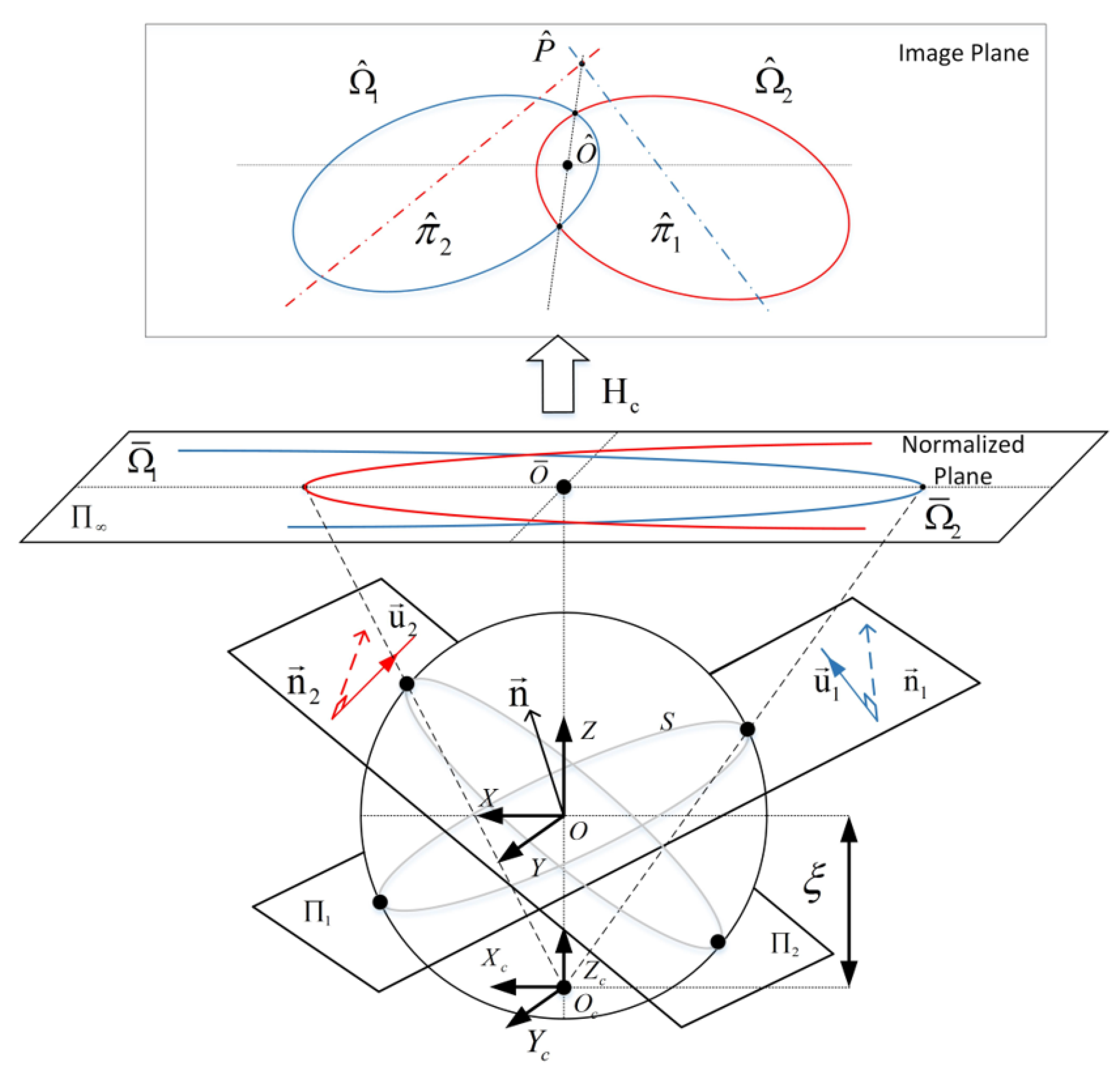
2.1. Line Image of Single 3D Line
2.2. Line Images of Two 3D Parallel Lines
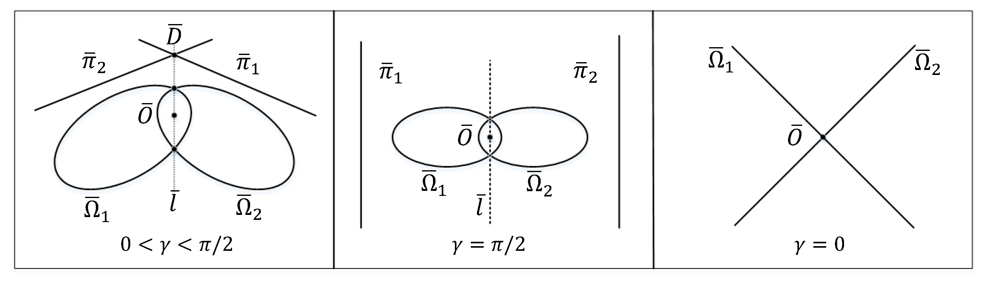
- and intersect at , if .
- The polar lines and are two vertical parallel lines, and will be infinite, if or .
- and will degenerate into two straight lines so that , if .
3. IBVS for Corridor-Following
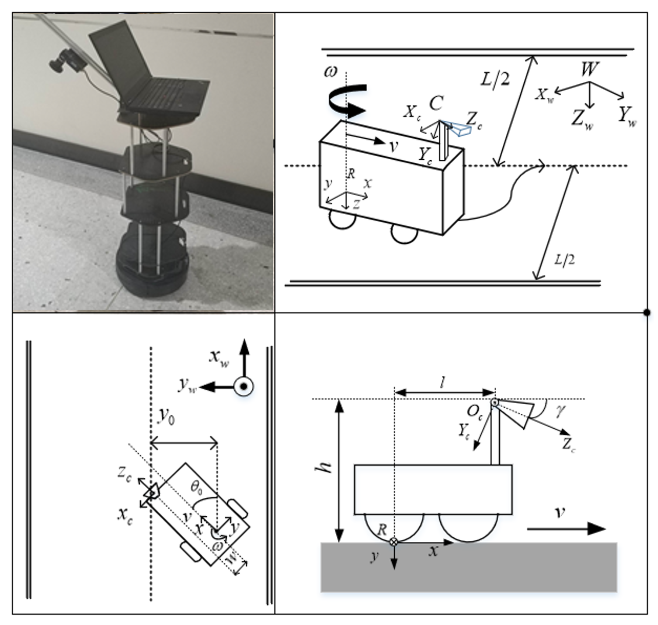
3.1. Modeling of Mobile Robot
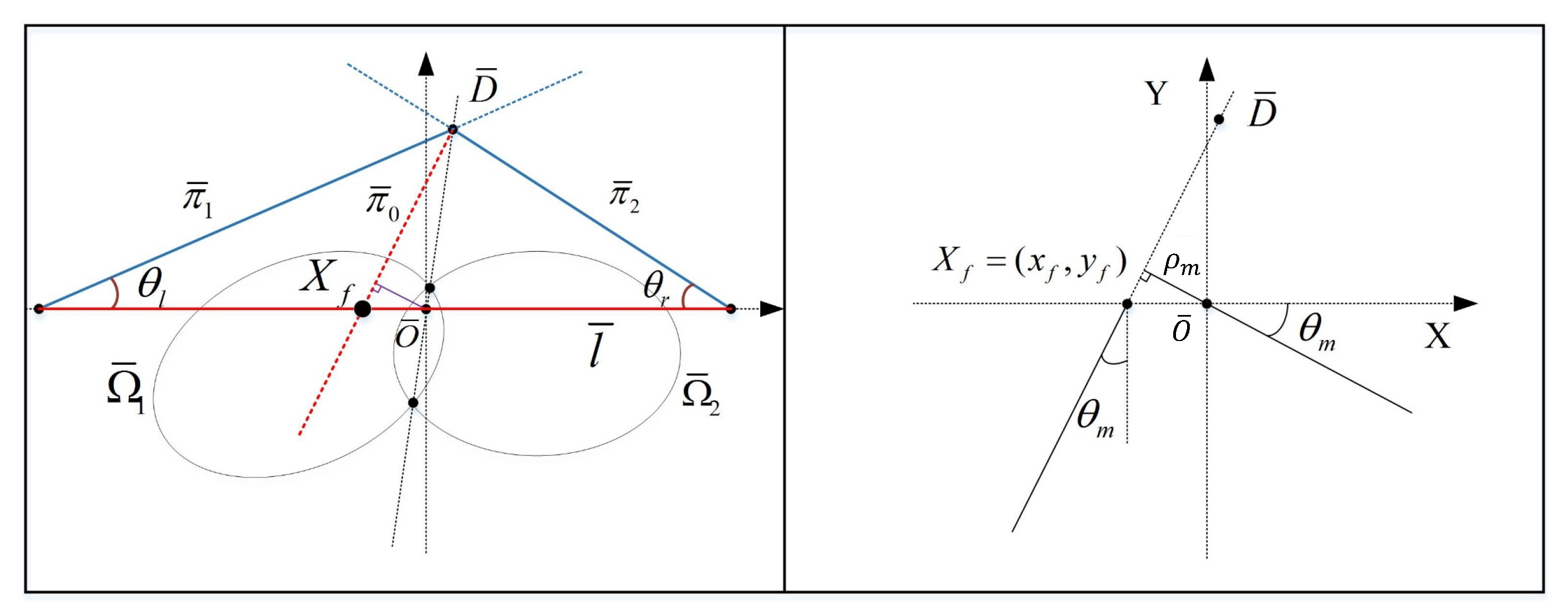
3.2. Visual Features for Corridor Horizon Lines
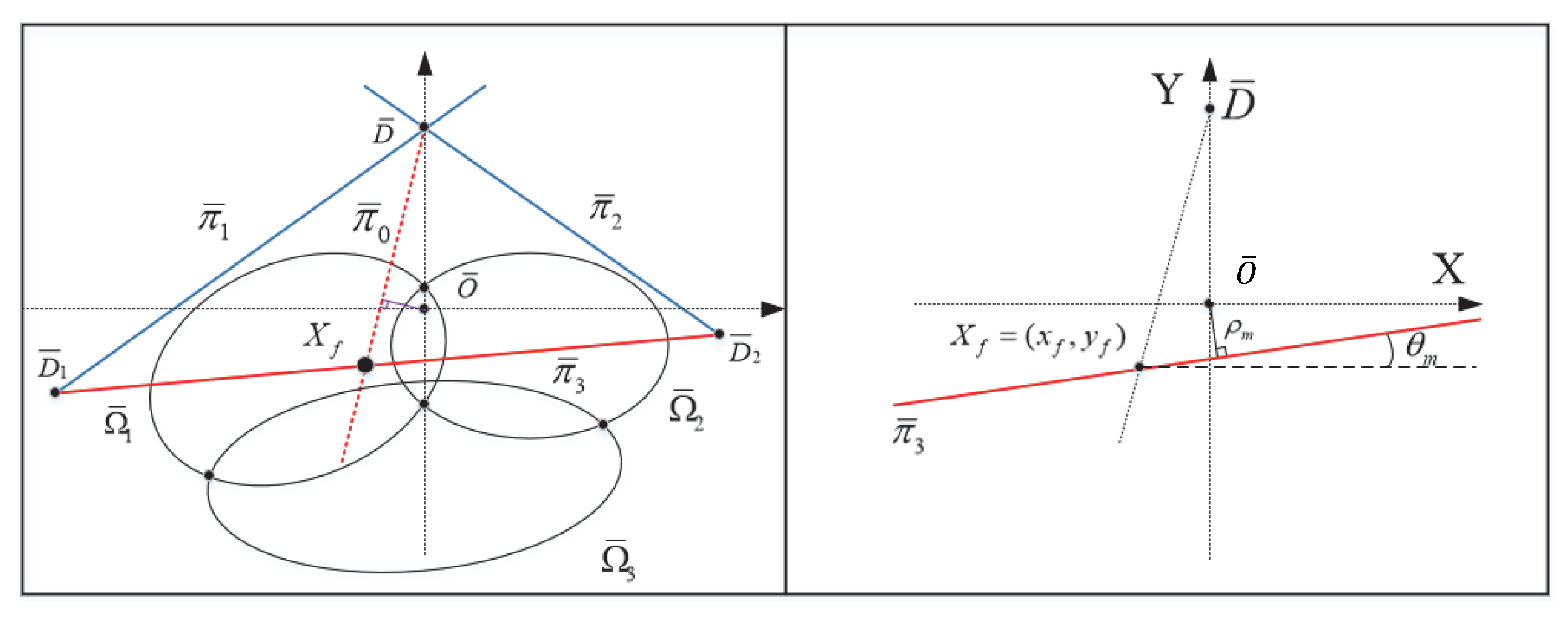
3.3. Visual Features for Doorway Vertical Lines
3.4. IBVS Control Law
3.5. Convergency Analysis
3.5.1. Corridor-Following Framework
3.5.2. Doorway-Passing
4. Simulation Results
4.1. Simulation for Corridor-Following
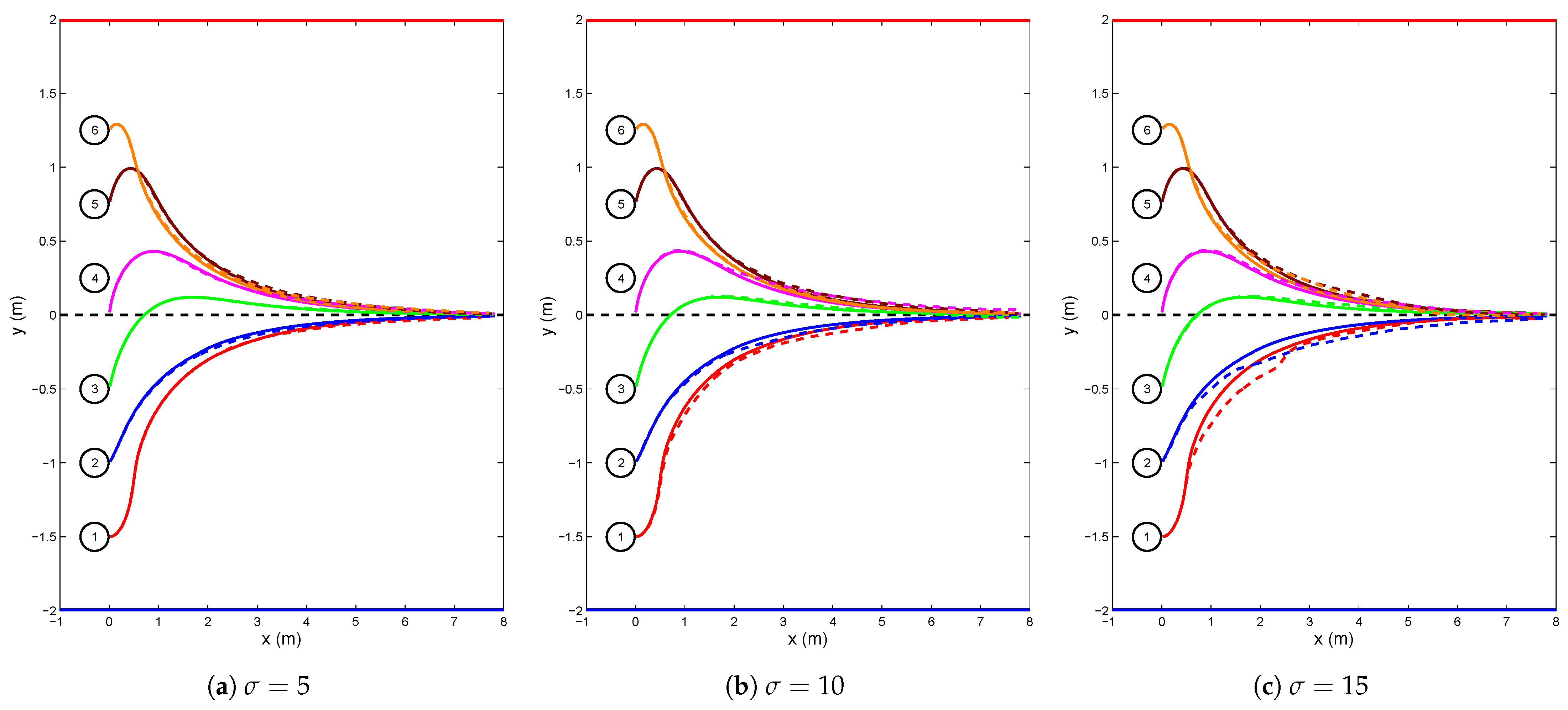
4.2. Anti-Noise Capability
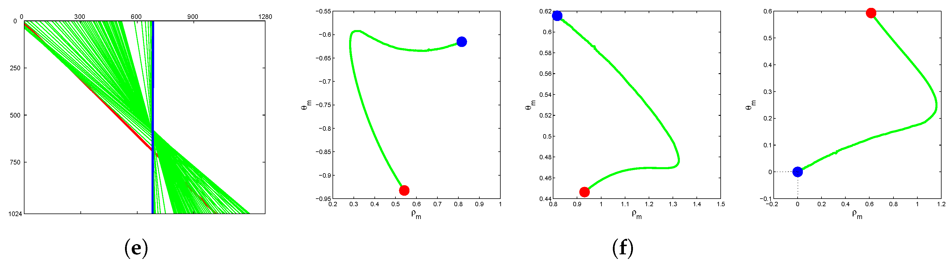
4.3. Convergence of Control Law
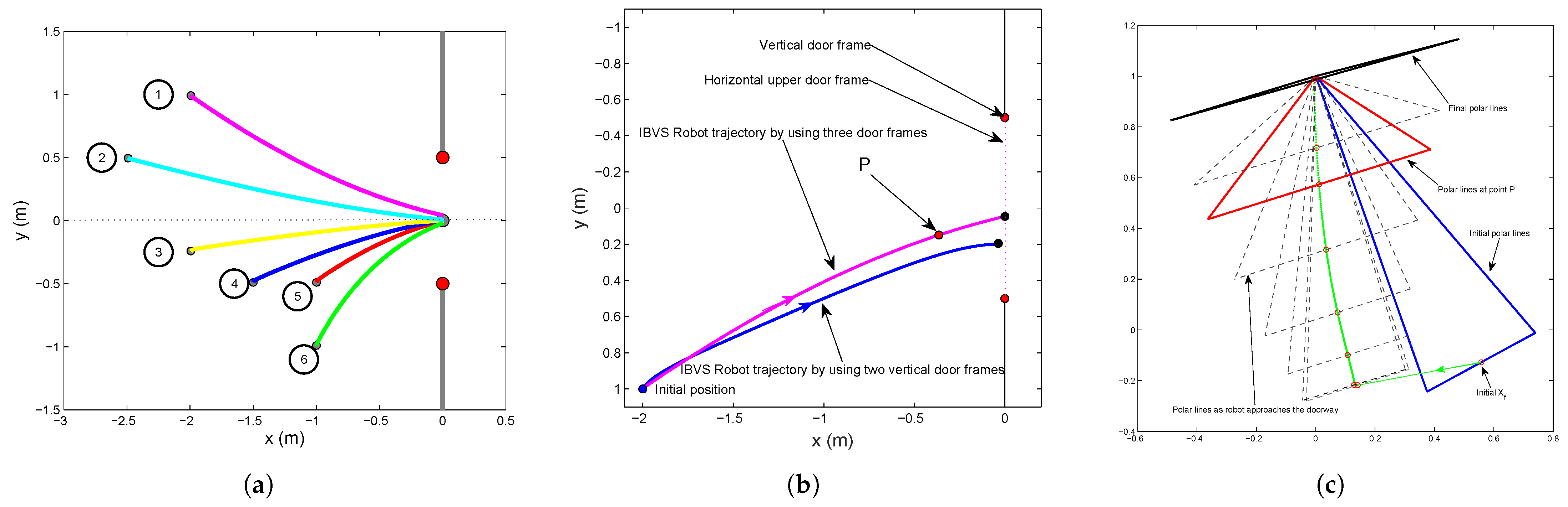
4.4. Simulation for Doorway Approaching
4.5. Simulation in Closed-Loop Corridor
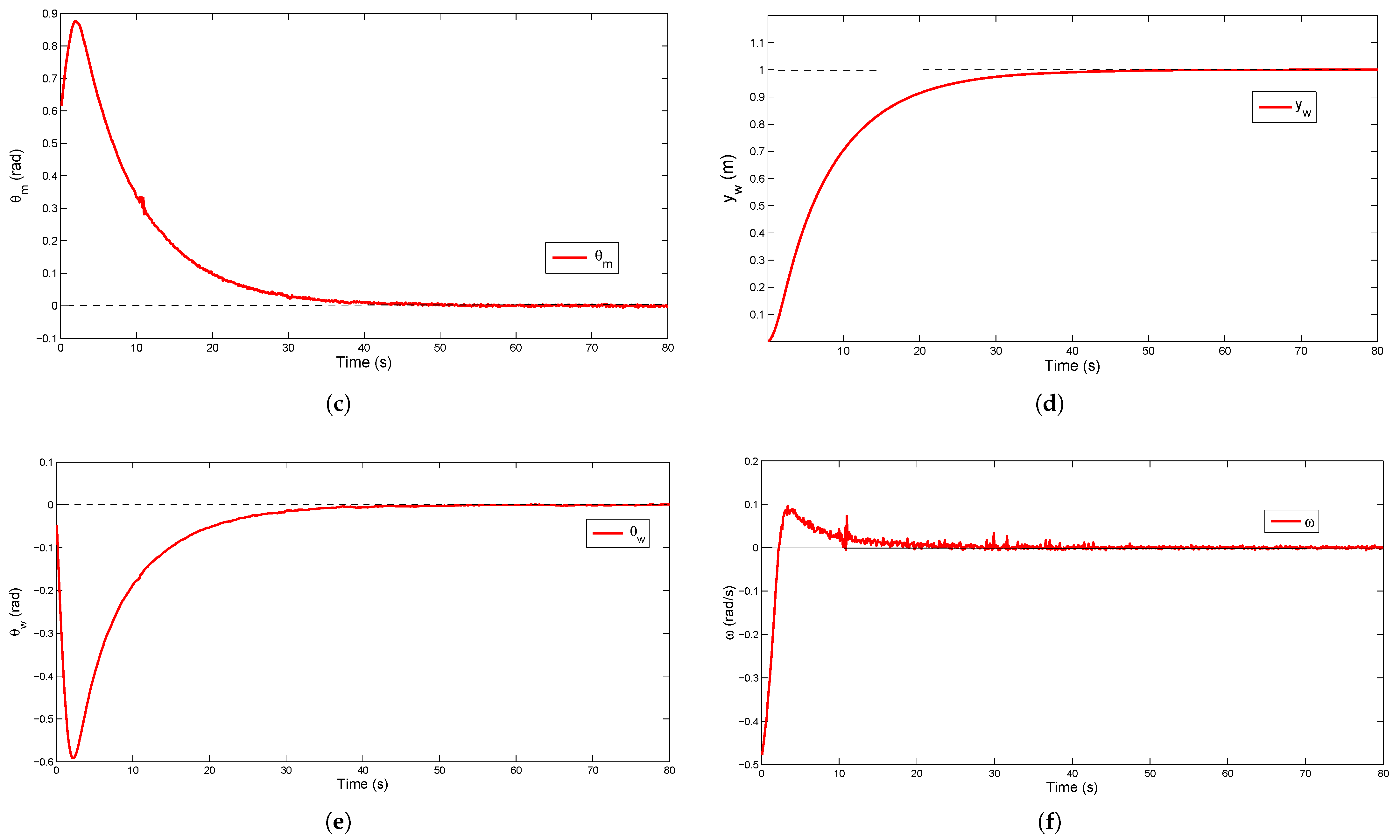
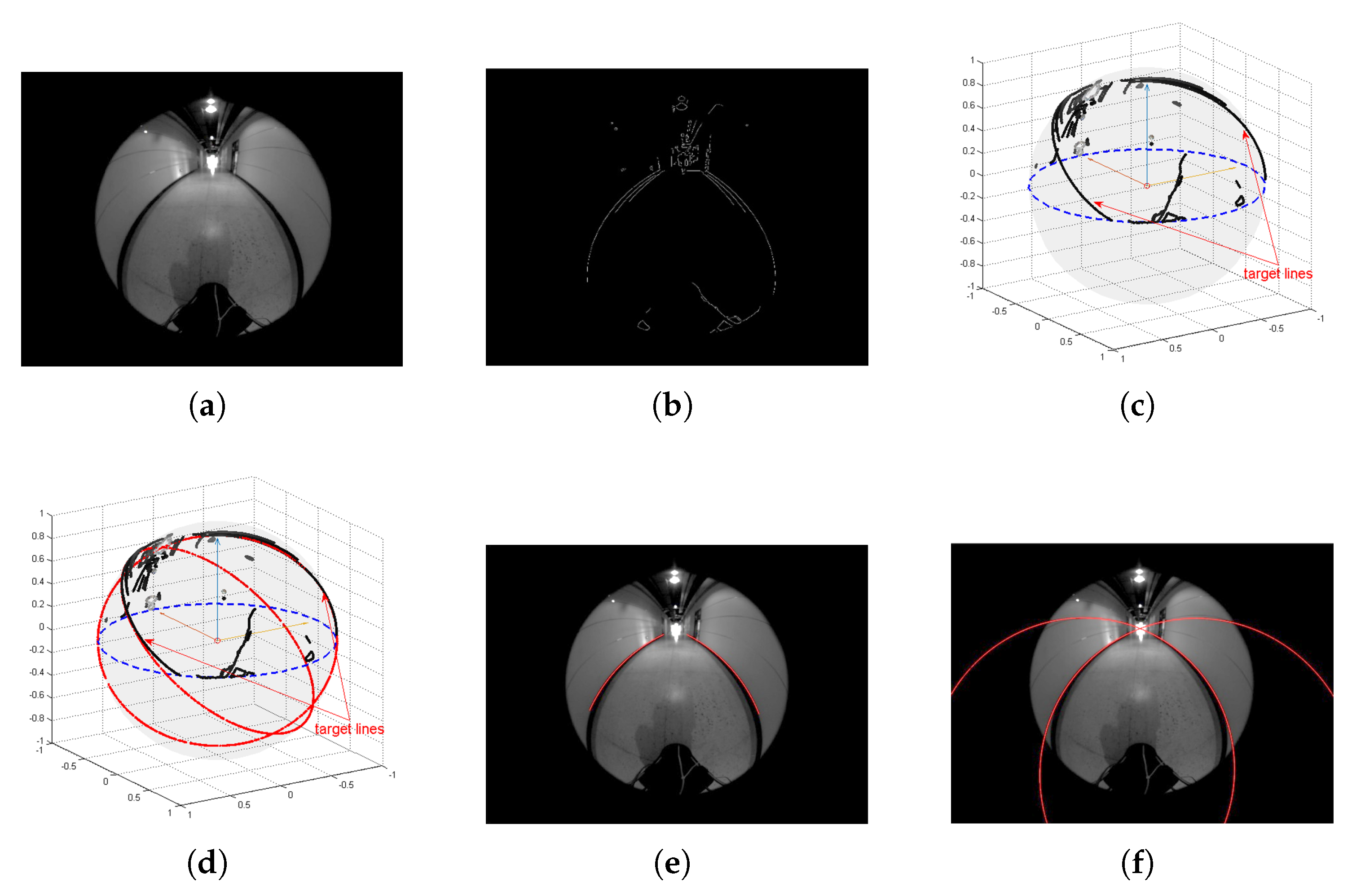
5. Experimental Results
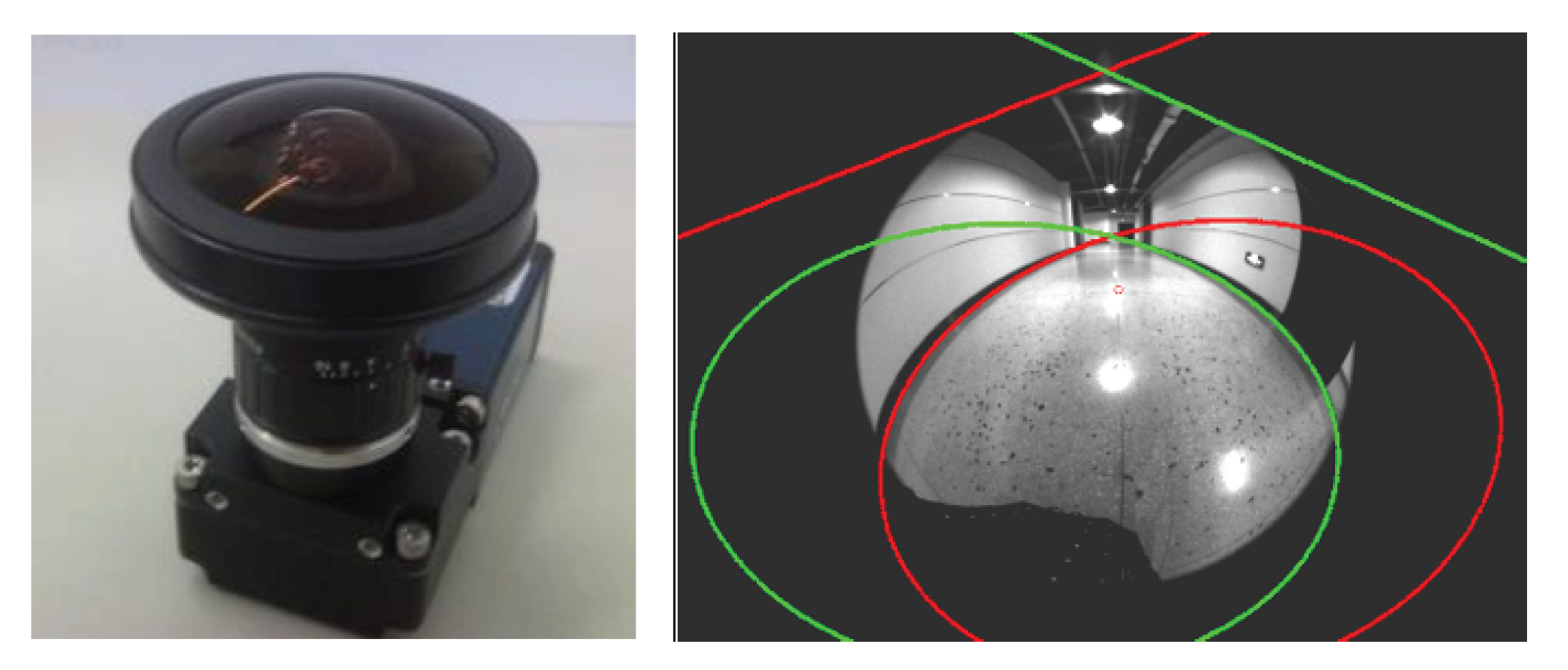
5.1. Mobile Robot Platform
5.2. IBVS System
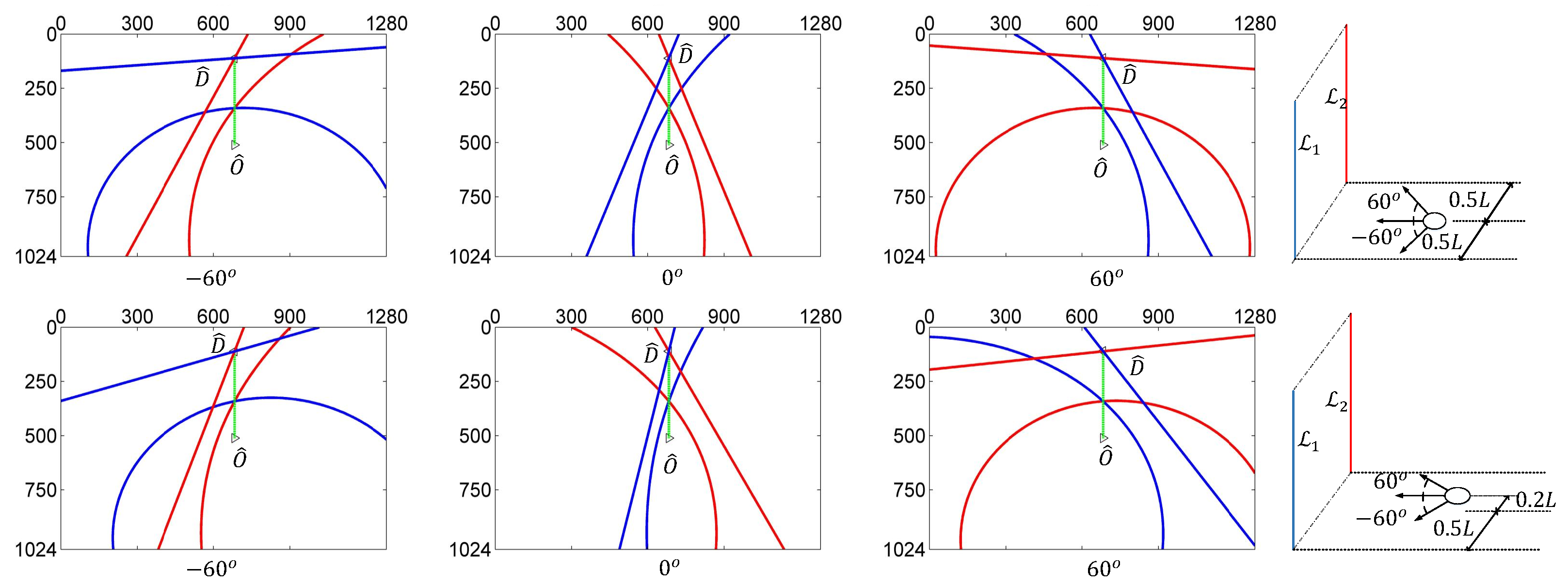
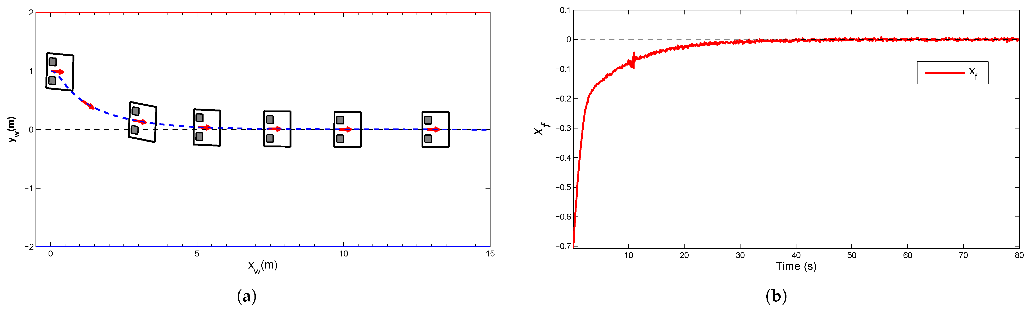
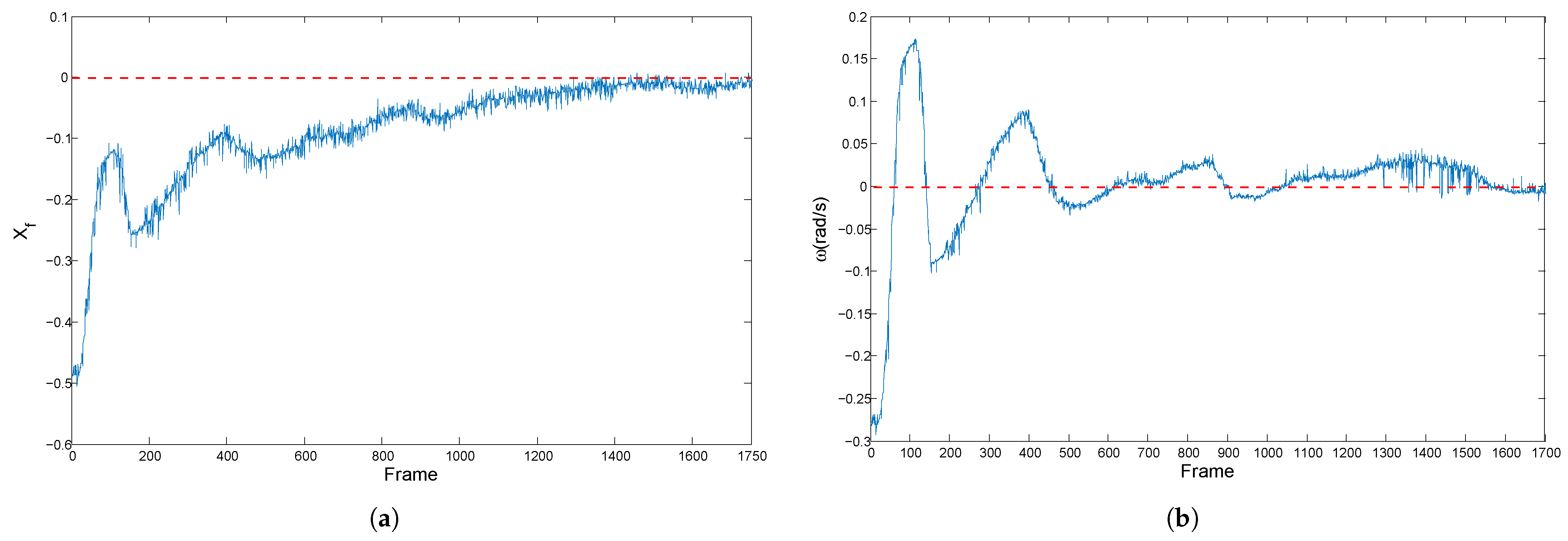
5.3. Experimental Results for Corridor-Following
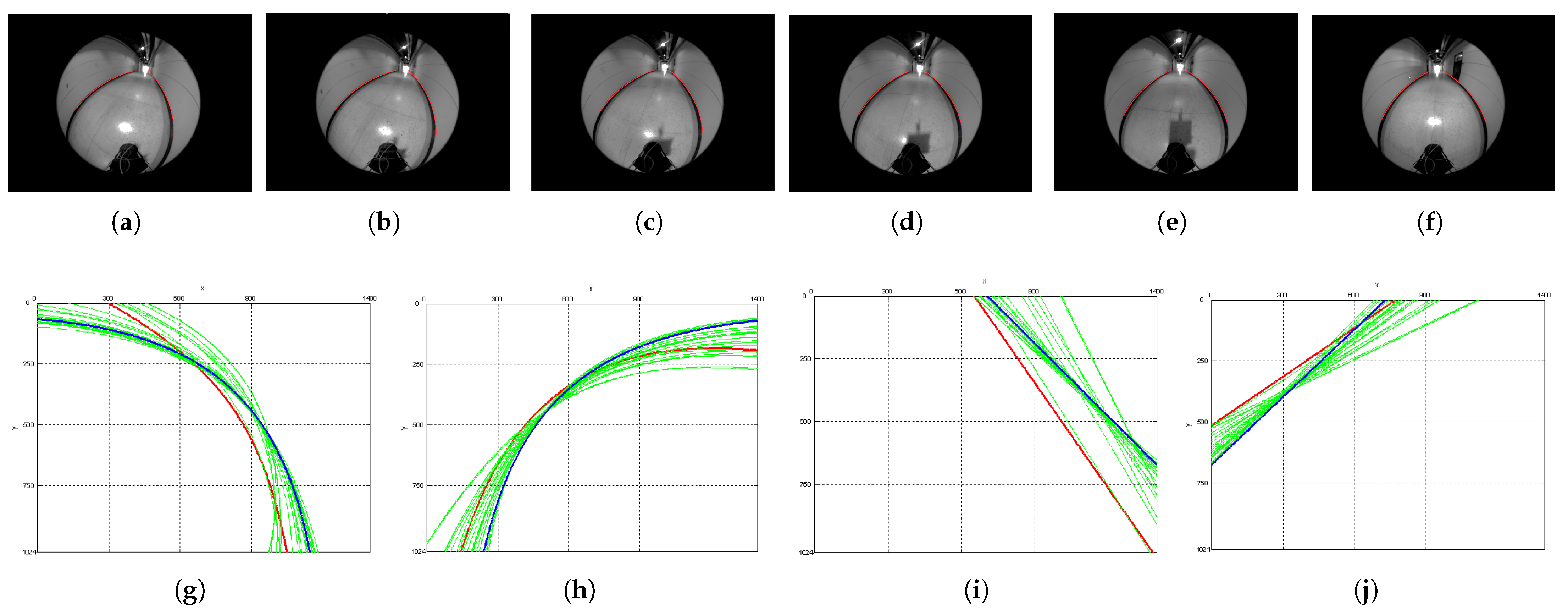
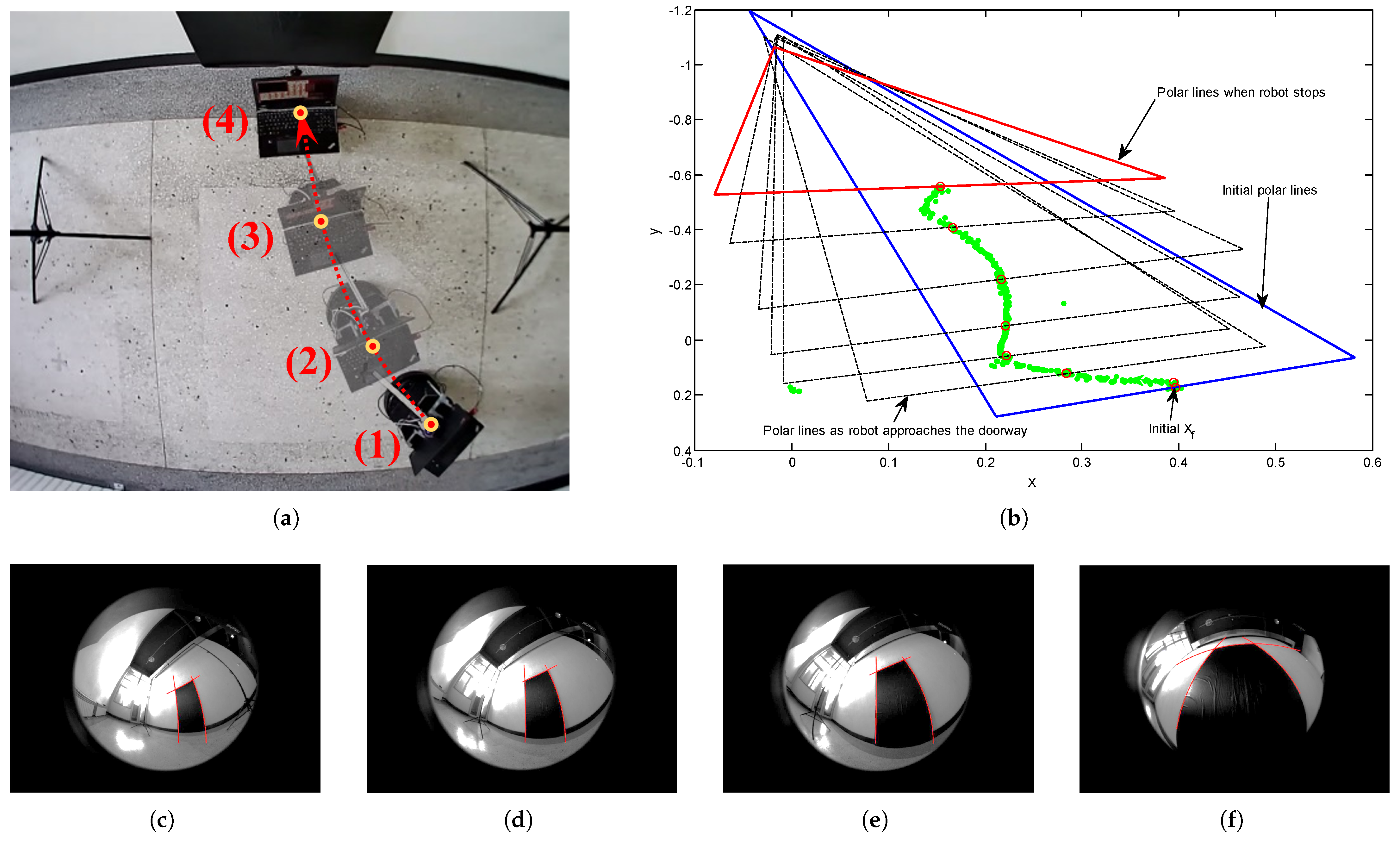
5.4. Experimental Results for Doorway-Passing
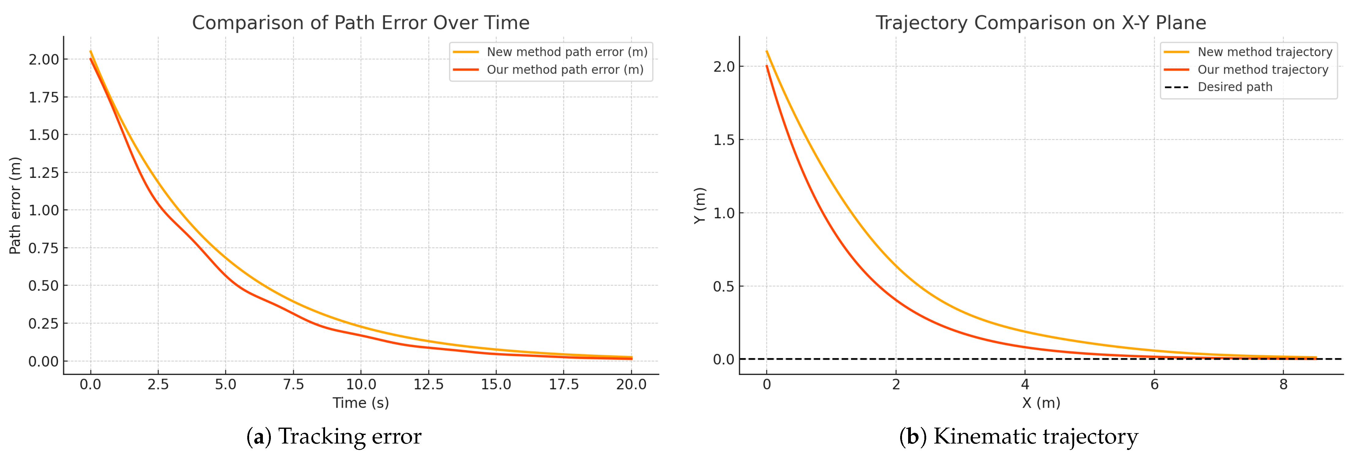
5.5. Experimental Results for Contrast
6. Conclusions
Author Contributions
Funding
Data Availability Statement
Conflicts of Interest
References
- Narayanan, V.K.; Pasteau, F.; Marchal, M.; Krupa, A.; Babel, M. Vision-based adaptive assistance and haptic guidance for safe wheelchair corridor following. Comput. Vis. Image Underst. 2016, 149, 171–185. [Google Scholar] [CrossRef]
- Huang, Y.; Su, J. Visual servoing of nonholonomic mobile robots: A review and a novel perspective. IEEE Access 2019, 7, 134968–134977. [Google Scholar] [CrossRef]
- Cherubini, A.; Chaumette, F.; Oriolo, G. Visual servoing for path reaching with nonholonomic robots. Robotica 2011, 29, 1037–1048. [Google Scholar] [CrossRef]
- de Lima, D.A.; Victorino, A.C. A hybrid controller for vision-based navigation of autonomous vehicles in urban environments. IEEE Trans. Intell. Transp. Syst. 2016, 17, 2310–2323. [Google Scholar] [CrossRef]
- Rafique, M.A.; Lynch, A.F. Output-feedback image-based visual servoing for multirotor unmanned aerial vehicle line following. IEEE Trans. Aerosp. Electron. Syst. 2020, 56, 3182–3196. [Google Scholar] [CrossRef]
- Alshahir, A.; Kaaniche, K.; Albekairi, M.; Alshahr, S.; Mekki, H.; Sahbani, A.; Alanazi, M.D. An Advanced IBVS-Flatness Approach for Real-Time Quadrotor Navigation: A Full Control Scheme in the Image Plane. Machines 2024, 12, 350. [Google Scholar] [CrossRef]
- Pasteau, F.; Narayanan, V.K.; Babel, M.; Chaumette, F. A visual servoing approach for autonomous corridor following and doorway passing in a wheelchair. Robot. Auton. Syst. 2016, 75, 28–40. [Google Scholar] [CrossRef]
- Corke, P. Robotics, Vision and Control: Fundamental Algorithms in MATLAB; Springer: Berlin/Heidelberg, Germany, 2011. [Google Scholar]
- Chaumette, F.; Hutchinson, S. Visual servo control. I. Basic approaches. IEEE Robot. Autom. Mag. 2006, 13, 82–90. [Google Scholar] [CrossRef]
- Liu, S.; Dong, J. Robust online model predictive control for image-based visual servoing in polar coordinates. Trans. Inst. Meas. Control 2020, 42, 890–903. [Google Scholar] [CrossRef]
- Luy, N.T. Robust adaptive dynamic programming based online tracking control algorithm for real wheeled mobile robot with omni-directional vision system. Trans. Inst. Meas. Control 2017, 39, 832–847. [Google Scholar] [CrossRef]
- Li, L.; Liu, Y.H.; Jiang, T.; Wang, K.; Fang, M. Adaptive trajectory tracking of nonholonomic mobile robots using vision-based position and velocity estimation. IEEE Trans. Cybern. 2017, 48, 571–582. [Google Scholar] [CrossRef] [PubMed]
- Kang, Z.; Zou, W.; Ma, H.; Zhu, Z. Adaptive trajectory tracking of wheeled mobile robots based on a fish-eye camera. Int. J. Control. Autom. Syst. 2019, 17, 2297–2309. [Google Scholar] [CrossRef]
- Li, C.L.; Cheng, M.Y.; Chang, W.C. Dynamic performance improvement of direct image-based visual servoing in contour following. Int. J. Adv. Robot. Syst. 2018, 15, 1729881417753859. [Google Scholar] [CrossRef]
- Yu, Q.; Wei, W.; Wang, D.; Li, Y.; Gao, Y. A Framework for IBVS Using Virtual Work. Actuators 2024, 13, 181. [Google Scholar] [CrossRef]
- Pan, L.; Li, W.; Zhu, J.; Zhao, J.; Liu, Z. Accurate and Fast Fire Alignment Method Based on a Mono-binocular Vision System. Fire Technol. 2024, 60, 401–429. [Google Scholar] [CrossRef]
- Zhang, X.; Fang, Y.; Li, B.; Wang, J. Visual servoing of nonholonomic mobile robots with uncalibrated camera-to-robot parameters. IEEE Trans. Ind. Electron. 2016, 64, 390–400. [Google Scholar] [CrossRef]
- Liang, X.; Wang, H.; Liu, Y.H.; Chen, W.; Jing, Z. Image-based position control of mobile robots with a completely unknown fixed camera. IEEE Trans. Autom. Control 2018, 63, 3016–3023. [Google Scholar] [CrossRef]
- Liang, X.; Wang, H.; Liu, Y.H.; Liu, Z.; You, B.; Jing, Z.; Chen, W. Purely image-based pose stabilization of nonholonomic mobile robots with a truly uncalibrated overhead camera. IEEE Trans. Robot. 2020, 36, 724–742. [Google Scholar] [CrossRef]
- Salaris, P.; Vassallo, C.; Soueres, P.; Laumond, J.P. Image-based control relying on conic curves foliation for passing through a gate. In Proceedings of the 2015 IEEE International Conference on Robotics and Automation (ICRA), Seattle, WA, USA, 26–30 May 2015; pp. 684–690. [Google Scholar]
- Bista, S.R.; Giordano, P.R.; Chaumette, F. Appearance-based indoor navigation by IBVS using line segments. IEEE Robot. Autom. Lett. 2016, 1, 423–430. [Google Scholar] [CrossRef]
- Bista, S.R.; Giordano, P.R.; Chaumette, F. Combining line segments and points for appearance-based indoor navigation by image based visual servoing. In Proceedings of the 2017 IEEE/RSJ International Conference on Intelligent Robots and Systems (IROS), Vancouver, BC, Canada, 24–28 September 2017; pp. 2960–2967. [Google Scholar]
- Chen, Z.; Li, T.; Jiang, Y. Image-based visual servoing with collision-free path planning for monocular vision-guided assembly. IEEE Trans. Instrum. Meas. 2024, 73, 7508717. [Google Scholar] [CrossRef]
- Dong, J.; Li, Y.; Wang, B. Image-based visual servoing with Kalman filter and swarm intelligence optimisation algorithm. Proc. Inst. Mech. Eng. Part I J. Syst. Control Eng. 2024, 238, 820–834. [Google Scholar] [CrossRef]
- Dorbala, V.S.; Hafez, A.A.; Jawahar, C. A deep learning approach for robust corridor following. In Proceedings of the 2019 IEEE/RSJ International Conference on Intelligent Robots and Systems (IROS), Macau, China, 3–8 November 2019; pp. 3712–3718. [Google Scholar]
- Fu, G.; Xiong, G.; Wang, Y.; Cheng, P.; Deng, W.; Tao, R. Research on Forest Fire Target Detection and Tracking Based on Drones. In Proceedings of the 3rd International Conference on Computer, Artificial Intelligence and Control Engineering, Xi’an, China, 26–28 January 2024; pp. 610–614. [Google Scholar]
- da Silva, A.F.; Araújo, A.F.; Durand-Petiteville, A.; Mendes, C.S. Feature Descriptor based on Differential Evolution for Visual Navigation in Dynamic Environments. IFAC-PapersOnLine 2023, 56, 5041–5046. [Google Scholar] [CrossRef]
- Tsapin, D.; Pitelinskiy, K.; Suvorov, S.; Osipov, A.; Pleshakova, E.; Gataullin, S. Machine learning methods for the industrial robotic systems security. J. Comput. Virol. Hacking Tech. 2024, 20, 397–414. [Google Scholar] [CrossRef]
- Jokić, A.; Jevtić, Đ.; Brenjo, K.; Petrović, M.; Miljković, Z. Deep Learning-based Visual Servoing Algorithm For Wheeled Mobile Robot Control. In Proceedings of the 15th INTERNATIONAL SCIENTIFIC CONFERENCE MMA2024-FLEXIBLE TECHNOLOGIES, Novi Sad, Serbia, 24–26 September 2024; pp. 71–74. [Google Scholar]
- Bechlioulis, C.P.; Heshmati-Alamdari, S.; Karras, G.C.; Kyriakopoulos, K.J. Robust image-based visual servoing with prescribed performance under field of view constraints. IEEE Trans. Robot. 2019, 35, 1063–1070. [Google Scholar] [CrossRef]
- Bista, S.R.; Ward, B.; Corke, P. Image-based indoor topological navigation with collision avoidance for resource-constrained mobile robots. J. Intell. Robot. Syst. 2021, 102, 55. [Google Scholar] [CrossRef]
- Hadj-Abdelkader, H.; Mezouar, Y.; Andreff, N.; Martinet, P. Omnidirectional visual servoing from polar lines. In Proceedings of the 2006 IEEE International Conference on Robotics and Automation, 2006. ICRA 2006, Orlando, FL, USA, 15–19 May 2006; pp. 2385–2390. [Google Scholar]
- Hadj-Abdelkader, H.; Mezouar, Y.; Martinet, P.; Chaumette, F. Catadioptric visual servoing from 3-d straight lines. IEEE Trans. Robot. 2008, 24, 652–665. [Google Scholar] [CrossRef]
- Mariottini, G.L.; Prattichizzo, D. Image-based visual servoing with central catadioptric cameras. Int. J. Robot. Res. 2008, 27, 41–56. [Google Scholar] [CrossRef]
- Marie, R.; Said, H.B.; Stéphant, J.; Labbani-Igbida, O. Visual servoing on the generalized voronoi diagram using an omnidirectional camera. J. Intell. Robot. Syst. 2019, 94, 793–804. [Google Scholar] [CrossRef]
- Junior, J.M.; Tommaselli, A.; Moraes, M. Calibration of a catadioptric omnidirectional vision system with conic mirror. ISPRS J. Photogramm. Remote Sens. 2016, 113, 97–105. [Google Scholar] [CrossRef]
- Barreto, J.P.; Araujo, H. Fitting conics to paracatadioptric projections of lines. Comput. Vis. Image Underst. 2006, 101, 151–165. [Google Scholar] [CrossRef]
- Torii, A.; Imiya, A. The randomized-Hough-transform-based method for great-circle detection on sphere. Pattern Recognit. Lett. 2007, 28, 1186–1192. [Google Scholar] [CrossRef]
- Albekairi, M.; Mekki, H.; Kaaniche, K.; Yousef, A. An Innovative Collision-Free Image-Based Visual Servoing Method for Mobile Robot Navigation Based on the Path Planning in the Image Plan. Sensors 2023, 23, 9667. [Google Scholar] [CrossRef]


| State | ① | ② | ③ | ④ | ⑤ | ⑥ |
| (degree) | 0 | 30 | 60 | 80 | 60 | 30 |
| (m) | −1.5 | −1 | −0.5 | 0 | 0.75 | 1.5 |
| Noise Level (Pixel) | MSE of Steady State (cm) |
|---|---|
| 5 | |
| 10 | |
| 15 | |
| 20 |
| State | ① | ② | ③ | ④ | ⑤ | ⑥ |
| (degree) | 0 | 30 | 60 | 80 | 60 | 30 |
| (m) | −1.5 | −1 | −0.5 | 0 | 0.75 | 1.5 |
| (m) | 1 | 0.5 | −0.25 | −0.5 | −0.5 | −1 |
| Error (cm) | 4.02 | 0.70 | 0.11 | 0.19 | 0.23 | 1.89 |
Disclaimer/Publisher’s Note: The statements, opinions and data contained in all publications are solely those of the individual author(s) and contributor(s) and not of MDPI and/or the editor(s). MDPI and/or the editor(s) disclaim responsibility for any injury to people or property resulting from any ideas, methods, instructions or products referred to in the content. |
© 2025 by the authors. Licensee MDPI, Basel, Switzerland. This article is an open access article distributed under the terms and conditions of the Creative Commons Attribution (CC BY) license (https://creativecommons.org/licenses/by/4.0/).
Share and Cite
Zhong, C.; Kong, Q.; Wang, K.; Zhang, Z.; Cheng, L.; Liu, S.; Han, L. Central Dioptric Line Image-Based Visual Servoing for Nonholonomic Mobile Robot Corridor-Following and Doorway-Passing. Actuators 2025, 14, 183. https://doi.org/10.3390/act14040183
Zhong C, Kong Q, Wang K, Zhang Z, Cheng L, Liu S, Han L. Central Dioptric Line Image-Based Visual Servoing for Nonholonomic Mobile Robot Corridor-Following and Doorway-Passing. Actuators. 2025; 14(4):183. https://doi.org/10.3390/act14040183
Chicago/Turabian StyleZhong, Chen, Qingjia Kong, Ke Wang, Zhe Zhang, Long Cheng, Sijia Liu, and Lizhu Han. 2025. "Central Dioptric Line Image-Based Visual Servoing for Nonholonomic Mobile Robot Corridor-Following and Doorway-Passing" Actuators 14, no. 4: 183. https://doi.org/10.3390/act14040183
APA StyleZhong, C., Kong, Q., Wang, K., Zhang, Z., Cheng, L., Liu, S., & Han, L. (2025). Central Dioptric Line Image-Based Visual Servoing for Nonholonomic Mobile Robot Corridor-Following and Doorway-Passing. Actuators, 14(4), 183. https://doi.org/10.3390/act14040183