Design of Experiments Approach for Structural Optimization of Urban Air Mobility Vehicles

Abstract

The current global context demands the development of new solutions that prioritize energy efficiency, time optimization, safety, and sustainability. Urban transportation is one of the sectors undergoing significant transformation. Pursuing new urban transportation solutions has become increasingly intense, involving research institutions and companies. Considering this context, this study focused on the optimization procedures for designing a new vehicle capable of vertical take-off for urban air mobility applications. This paper reports on the optimization process of a thruster deployment mechanism using statistical techniques. In particular, the authors tested the use of Design of Experiments (DOE) techniques for the optimal design of a structural component of a new vehicle for urban mobility purposes under development at the Applied Mechanics laboratory of the Department of Industrial Engineering of the University of Salerno. For this reason, it was decided that a parametric multibody model would be developed in the Simscape Multibody environment for structural optimization using designed experiment plans to “guide” the designer in the analysis phase and search for an optimal configuration using a minimum number of configurations. Finally, employing FEM analysis, the chosen configuration was validated. This study allowed us to test the use of DOE techniques to design new systems. It allowed us to evaluate different configurations, the static and dynamic behavior, the constraining reactions present in the joints, and the active forces and torques of the actuators, highlighting the correlation between factors that can guide the designer in identifying optimal solutions.

1. Introduction

Urban air mobility (UAM) is emerging as a key solution to address urban mobility challenges to create a more sustainable and connected transportation system. In Italy, too, UAM is rapidly evolving thanks to numerous initiatives and pilot projects [1,2]. Several collaborations involve leading aviation and airport companies, as illustrated in the following examples. Airbus and ITA Airways have signed a Memorandum of Understanding to develop urban air mobility services in Italy [3]. This agreement includes the introduction of the CityAirbus NextGen, an electric vertical take-off and landing (eVTOL) aircraft designed to carry up to four passengers on zero-emission flights. The goal is to create pilot cases to demonstrate the added value of UAM to local communities. In addition, ITA Airways and Airbus have extended their collaboration to include UrbanV and Enel, forming a strategic alliance for the development of the Advanced Air Mobility (AAM) ecosystem in Italy [4]. UrbanV will be responsible for managing the vertiport network, while Enel will provide technology solutions. This partnership will explore business models, standardize ground services, and plan the vertiport network while defining the passenger experience. Another significant initiative is the collaboration between Atlantia, Aeroporti di Roma, and Volocopter. This partnership aims to introduce electric air cabs to Rome. Volocopter has already presented the VoloCity at several public exhibitions in the Italian capital, highlighting the potential of these vehicles to improve urban mobility. As can be seen, recent technological advances have facilitated the emergence of urban air mobility (UAM), which involves the use of vertical take-off and landing (VTOL) aircraft to transport passengers within an urban area [5]. From this perspective, and with the need to develop green solutions, optimizing the aircraft’s structure and the actuators’ performance becomes vital [6,7]. In addition to the usual virtual design techniques, the authors tested statistical methods generally used to optimize production processes. For this purpose, a flexible parametric multibody model was created to test different combinations to optimize the constraint reactions and the active forces to be delivered by the electroactuators. In this paper, we describe how a multibody analysis was performed by using the multidominion Simscape environment of the Matlab R2023b Mathworks software [8,9]. This study is of paramount importance because it highlights the benefits obtainable by integrating multibody analysis with the use of the Design of Experiments (DOE), a statistical technique used to plan, conduct, analyze, and interpret experiments to reveal the actual correlation between parameters and arrive at their optimization in a guided manner [10]. Thus, it enables the investigation and optimization of products and processes by identifying critical factors affecting quality, reducing variability, defects, and waste. By designing well-structured experiments, cause-and-effect relationships between variables can be identified, and critical factors can be optimized. This approach makes it possible to determine whether a factor has a significant impact on the response, to analyze the interactions between factors, and to model response behavior as a function of the factors themselves. The DOE is a critically important tool in engineering because it enables evidence-based decision-making, improves process efficiency and quality, and reduces the overall costs. More and more companies are applying this technique, such as Ford in the automotive sector to optimize manufacturing processes and improve vehicle performance [11] and Boeing and Airbus in the aerospace sector for aircraft design and production to reduce manufacturing defects and improve safety and comfort [12,13].

The Design of Experiments (DOE) can also be used in combination with other advanced methodologies, such as Machine Learning (ML), for example, to optimize industrial experiments, with a focus on innovation and the development of new materials, such as amorphous metal alloys [14]. In addition, the DOE can be integrated with Computational Fluid Dynamics (CFD) techniques, for example, to optimize the shape of complex structures, such as the bow shape of an oil tanker hull. In the latter case, the DOE supports the reduction of wave-induced drag, thus enabling the identification of an optimal slipway configuration that will improve the vessel’s overall performance [15].

For all these reasons, this paper focuses on designing and evaluating experiments for the structural optimization of urban air mobility vehicles, highlighting the potential benefits of this approach. The paper is structured as follows: Section 2 presents the Simscape multidomain simulation environment, where the parametric multibody model of the thruster arm was developed and tested, the statistical technique chosen for this application (DOE) for the guided design of experiments, and the static analysis performed through FEM analysis for the validation of the solution. Section 3 describes the numerical activity by specifying and estimating the most relevant parameters using the DOE technique. Next, the investigation results are presented and discussed in Section 4. Section 5 presents a discussion of the results, advantages, limitations, and prospects of the proposed method. Finally, the Conclusions highlight the main results of this research, along with its limitations and future research needs (Section 6).

2. Materials and Methods

2.1. Multibody Modeling in the Simscape Multidomain Environment

Multibody dynamics studies the behavior of interconnected rigid or flexible bodies, which may undergo large translational and rotational displacements. This field has led to the development of a large number of important multibody formalisms in the field of mechanics. Newton (free particles) and Euler (rigid body) considered a multibody system’s simplest bodies or elements. Euler introduced reaction forces between bodies. Later, a series of formalisms were derived, although we will only mention Lagrange’s formalisms based on minimal coordinates and a second formulation that introduces constraints [16]. The kinematic behavior depends on the absolute and relative joints present in the model. The geometry and absolute and relative joints strongly influence the kinematic behavior of a multibody model. Joints are categorized based on the motion they allow (degrees of freedom). On the other hand, dynamic behavior is influenced by the active forces and torques applied to the bodies, the constraint reactions, and the inertial actions. However, calculating the constraint forces is very complicated, and applying the Newton–Euler equation can be challenging. For these reasons, a specific formulation of the equations of motion for a multibody system is required [17]. Today, multibody systems play a crucial role in numerous engineering research fields, particularly in robotics and vehicle dynamics. The formalisms of multibody systems typically provide an algorithmic, computer-aided approach to modeling, analyzing, simulating, and optimizing the complex motion of potentially thousands of interconnected bodies. Simulating multibody systems presents a host of challenges due to a variety of factors:

• High-Degree-of-Freedom (DOF) Systems: Simulating a high-DOF system with many constraints can be complex. This is because, fundamentally, all system DOFs are dynamically coupled, so a constraint force acting on a part of the system generally affects the entire system. This leads many algorithms to use large-sized matrix operations or excessive numerical iterations. Engineers often grapple with a trade-off between the level of realism or fidelity of a model and the computational and human engineering effort required to define the elements within the simulation.
• The Complexity of Algorithms: Another challenge is the complexity of the algorithms used for simulation. The algorithms must be robust, analytically sound, and capable of handling under-actuated systems, flexible systems, linearization, diagonalized dynamics, and space manipulators. Accurate and Efficient Data Acquisition: One of the most important concerns in robotic simulation research is obtaining data that are accurate and efficient in terms of the computation time. This includes many factors, such as discrete-time integration, various types of constraints, friction, system-induced sparsity, and numerical algorithms.
• Subsystem-Based Simulation: To address these challenges, researchers have developed a novel subsystem-based simulation approach that is simple, modular, suitable for parallelization, and ensures solution consistency and accuracy.

Despite these challenges, multibody dynamics simulation is a powerful tool that allows engineers to observe the transient dynamics within a system, avoid the costs of physical testing by identifying potential design problems before an entire system is built, and explore how changes to the system materials and configuration can optimize performance. Simscape Multibody, formerly known as SimMechanics, is a specialized environment within MATLAB that provides a multibody simulation platform for 3D mechanical systems. This environment is particularly useful for modeling and simulating complex systems with highly irregular geometry and multiple degrees of freedom. The Simscape Multibody environment allows users to model multibody systems using blocks that represent bodies, joints, constraints, force elements, and sensors. It formulates and solves the equations of motion for the complete mechanical system. One of Simscape Multibody’s key features is its ability to import complete CAD assemblies into the model, including all masses, inertias, joints, constraints, and 3D geometry. This feature facilitates the creation of a digital twin of the system under investigation. Simscape Multibody also provides an automatically generated 3D animation that visualizes the system dynamics. This visualization can be invaluable in understanding the system’s behavior under various conditions. In addition to these features, Simscape Multibody aids in the development of control systems and testing of the system-level performance. Users can parameterize their models using MATLAB variables and expressions and design control systems for their multibody system in Simulink. Furthermore, Simscape Multibody allows for the integration of hydraulic, electrical, pneumatic, and other physical systems into the model using components from the Simscape family of products. Simscape Multibody supports C-code generation to facilitate the deployment of such complex and detailed models to other simulation environments, including hardware-in-the-loop (HIL) systems. This feature enables users to test control algorithms and run HIL tests on various real-time systems before performing physical tests. In conclusion, Simscape Multibody is a powerful tool for modeling, simulating, and analyzing 3D mechanical systems. Its wide range of features and capabilities make it an invaluable resource for engineers and researchers in various mechanical and control engineering fields.

2.2. Design of Experiments (DOE)

The Design of Experiments (DOE) is an advanced active statistical method that, instead of merely passively observing a phenomenon and recording empirical results, directly intervenes by changing the values of the system’s input parameters in a way that facilitates the significantly faster identification of the overall optimal solution compared to traditional methods. The DOE involves creating a symmetric distribution of experiments around the central point, where all factors are modified simultaneously. Such a method makes it possible to identify a direction, known as the gradient of the objective function, along which that function can be maximized or minimized, yielding productive results that are both better and more robust. Identifying and exploiting this optimal direction is crucial to improving the efficiency of the production process. Practical experimentation and the prototyping of the system are performed only at the end of the process to empirically validate the results obtained from previous simulations. Statistical programming methods for experiments, also known as the Design of Experiments (DOE), find application in a process’s development and fine-tuning phases, improving its performance and robustness against external variations. To ensure replicability and applicability to various production contexts, the methodology must be systematically structured and organized into chronological steps. 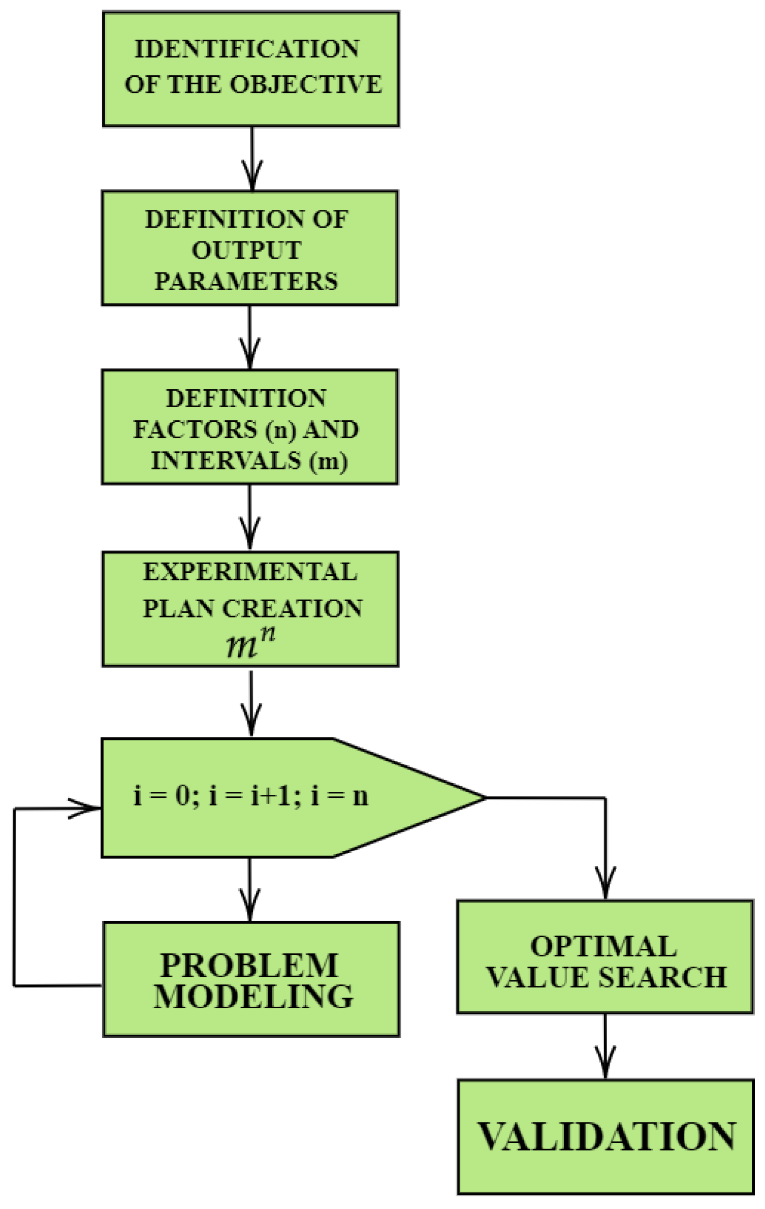The Figure 1 is a representation of flow of data. The planning of experiments is divided into eight basic steps:

1.

Recognition, problem formulation, and goal setting: Establish what will be obtained from the experiment. This step consists of the function definition containing the parameters considered fundamental to achieving the objective.

2.

Process variable selection: Identify the factors, i.e., the variables that can influence the results, and the levels, i.e., the values at which these factors appear during an experiment; these are the key components of the DOE. Thus, one identifies the factors that influence the production process and quality of a product, i.e., the most crucial factors, and identifies the optimal levels of these factors needed to obtain a product that is more reliable, durable, and easy to use than those of their competitors.

A distinction is made between controllable and uncontrollable factors:

• Controllable factors: The variables that can be directly manipulated during an experiment. They are varied systematically to study their effect on the output of the process.
• Uncontrollable factors: The variables that cannot be manipulated directly or controlled during the experiment must be managed to reduce their negative impact.

3.

The selection of a feasible experimental design: Decide on the number of replications and chronological order and choose from full factorial designs, fractional factorial designs, or response surfaces.

• Full factorial designs: These designs involve testing all possible combinations of factors; there is the complete collection of information. For example, if there were two factors with two levels each, there would be four possible combinations (2 × 2 = 4). Complete factorial designs are the most comprehensive but can be the most time-consuming and expensive.
• Fractional factorial designs: Fractional factorial experiments are a type of factorial experiment that uses fewer experimental runs than a complete factorial design. These designs involve testing a subset of the possible combinations of factors; in this case, the designer achieves the partial collection of information due to the few combinations monitored, reducing the cost and time taken to perform the tests. Fractional factorial designs are less complete than full factorial designs, but they can save time and money.

4.

Running the experiment: Conducting the planned experiments systematically by changing the factors and observing the results. A key component of this process is the ability to repeat the experiment to reduce variability and increase reliability.

5.

Data consistency validation: Data must be consistent with experimental hypotheses.

6.

The analysis and interpretation of the results: Use statistical methods to interpret the data, determine the importance of various factors, and draw statistically significant conclusions. So, the main objectives of this phase are as follows:

• Identify the main process factors affecting the system performance and variability.
• Determine the optimal levels of the variables of interest to ensure the best performance and the robustness of the outcome, i.e., minimizing the impact of uncontrollable variables.
• Evaluate, where possible, further system improvements from a technical and economic perspective.

7.

The presentation of the results and application of decision-making: There is an implementation of the changes, i.e., the results are applied to optimize the process or product.

8.

Conclusions: The validation of the selected solution.

Figure 1. Process outline.

Figure 1. Process outline.

These phases are often interconnected and iterative, especially in complex projects, where the results of one phase can influence decisions in the others. Benefits can be achieved through the application of these phases, for example, those described in [18]:

• The efficient use of resources:

  a.

  A reduction in the number of calculated configurations (experimental trials).

  b.

  The elimination of redundant configurations.

  c.

  More information on the possible relationships between variables and objectives.

• The statistical and scientific analysis of the system and understanding of the phenomenon.
• Reducing the cost of producing a product. By identifying the most efficient method of producing an optimized product using DOE methodologies, companies can improve the quality of their products and save on labor, material, and other associated costs. This can reduce the final price of the product, thus making it more competitive in the market.
• Increased efficiency and improved decision-making and developing new products that meet the needs of a specific market. By understanding the needs of the target market, companies can develop products that are more likely to succeed. This makes it easier for companies to enter new markets and increase their market share.
• Faster time to market.
• Improved control and quality. According to [18], quality assurance is process-oriented and is a management tool, while quality control is product-oriented and is a corrective tool. A powerful tool used in quality control and quality assurance is the Design of Experiments (DOE). Quality control and assurance are crucial aspects of any production or industrial process, essential to customer satisfaction and overall business success. Quality is a measure of the degree to which a product conforms to design specifications or the ability of a product or service to meet user requirements. Integrating quality assurance and quality control enables the delivery of a defect-free product or service.

DOE methodologies are increasingly being used in various applications, including new product design, design improvement, maintenance, manufacturing process control and improvement, and product maintenance and repair. This approach improves the product and process quality, reduces costs, and increases efficiency [18]. Thus, it can be argued that the Design of Experiments (DOE) is a powerful and versatile methodology that, through careful, systematic analysis, in-depth process understanding, and simulation, enables improvement while providing significant time and cost savings associated with design and experimentation within the production system, simultaneously improving the efficiency and effectiveness of production processes and the quality of the products produced [19]. The DOE aims to create an information framework that enables product or production process innovation and optimization. This goal is based not on sudden intuition but on adopting a repeatable, systematic, and standardized method. This approach achieves continuous and sustainable improvements by fostering a structured innovation process based on empirical data.

2.3. Use of Finite Element Analysis for Data Validation

Finite Element Method (FEM) analysis is a crucial tool in the design and development of new machines. This computational technique allows engineers to simulate and predict the behavior of complex structures under various conditions. By breaking down a large system into smaller, manageable elements, the FEM provides detailed insights into the stress distribution, deformation, and potential failure points. This method enhances the accuracy and efficiency of the design process, enabling the creation of more reliable and optimized machines. With FEM analysis, engineers can test different materials, geometries, and load conditions virtually, reducing the need for physical prototypes and accelerating the development cycle. Finite Element Method (FEM) analysis offers several key benefits in the design and development of new machines:

Accuracy: The FEM provides precise predictions of how a machine will behave under various conditions, helping to identify potential issues before they arise.

Efficiency: By simulating different scenarios virtually, the FEM reduces the need for physical prototypes, saving time and resources in the development process.

Optimization: Engineers can test various materials, geometries, and load conditions to find the most efficient and effective design solutions.

Risk Reduction: The FEM helps in identifying and mitigating potential failure points, enhancing the safety and reliability of the final product.

Cost Savings: By minimizing the need for physical testing and reducing the likelihood of design errors, the FEM can significantly lower development costs.

Flexibility: The FEM can be applied to a wide range of engineering problems, from those in simple components to those in complex systems, making it a versatile tool in machine design. Such an instrument can also validate design choices in several ways:

Stress and Strain Analysis: The FEM can simulate how a design will respond to various loads and forces, identifying areas of high stress and potential failure. This helps ensure that the design can withstand real-world conditions.

Deformation Prediction: By predicting how a structure will deform under load, the FEM helps verify that the design will maintain its shape and functionality throughout its lifecycle.

Thermal Analysis: The FEM can model the heat distribution and thermal stresses, ensuring that the design can handle temperature variations without compromising performance.

Dynamic Analysis: For designs subject to dynamic loads, such as vibrations or impacts, the FEM can simulate these conditions to validate that the design will perform reliably.

Material Optimization: The FEM allows engineers to test different materials and their properties, ensuring that the chosen material will provide the necessary strength, durability, and cost-effectiveness.

Safety Margins: By identifying the limits of a design’s performance, the FEM helps establish safety margins, ensuring that the design remains safe under unexpected conditions.

Compliance with Standards: The FEM can be used to verify that a design meets industry standards and regulations, providing confidence that the design is both safe and compliant.

Iterative Improvement: The FEM enables the iterative testing and refinement of a design, allowing engineers to make informed adjustments and improvements before finalizing the design.

3. Numerical Activity

3.1. Multibody Model of Actuation System

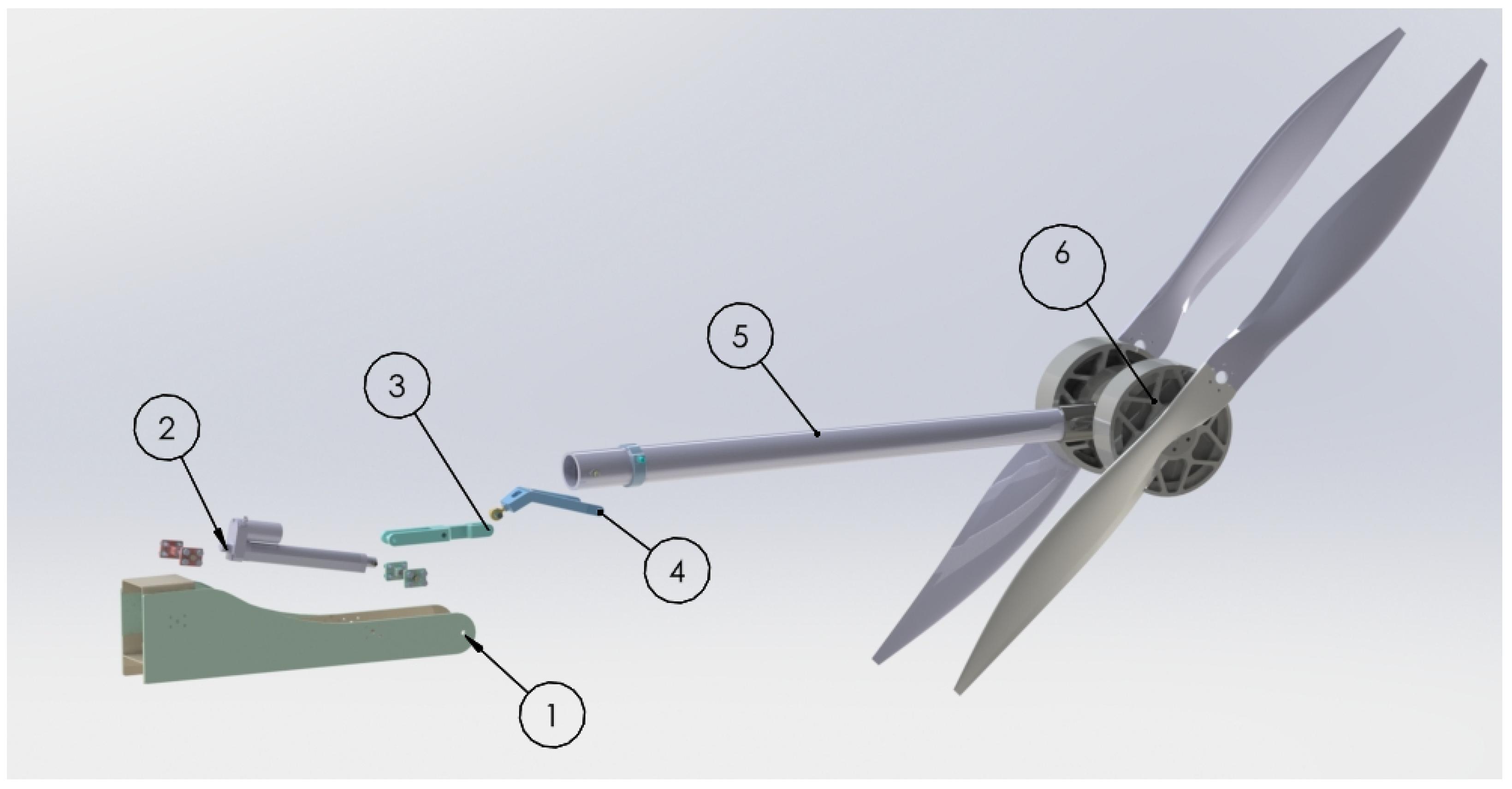
The aircraft’s thruster deployment mechanism was analyzed to test the optimization procedure. An exploded view of the components that make up the kinematic mechanism is shown in Figure 2, while information regarding the individual parts is reported in

Table 1. BOM of the components of the propulsor deployment mechanism.

Item	Part	Material	Mass
1	Rod	38NiCrMo4	$0.066$ kg
2	Linear Actuator (Bottom)	Aluminum	1 kg
3	Crank (Bottom)	38NiCrMo4	$0.93$ kg
4	Biella	38NiCrMo4	$0.980$ kg
5	Tube	Aluminum	$4.65$ kg
6	Propeller Actuator	38NiCrMo4	$3.86$ kg

. The vehicle has an estimated mass of about 450 kg for a payload of 150 kg. Therefore, a required lift of 5886 N is assumed during “hovering” (considering a tilt angle, $\theta$, equal to 0 deg). Such a value is estimated for a thrust that is equal to the total weight of the stationary vehicle in the air (v = 0 m/s) at a constant altitude and, in addition, with a vehicle configuration that involves a propulsion unit consisting of two motors arranged with coaxial propellers on each arm. The thrust generated by each propulsion unit on each arm is a quarter of the total thrust or 1471.5 N. The analysis extended to the maximum vertical thrust achieved by a single propulsion unit on a single arm, 2943 N. This value was obtained by adding an excess thrust of 100% to the total vertical “hovering” thrust to ensure the ability to perform several flight maneuvers meeting safety requirements. The analysis considered an alternative tilt angle, $\theta$, equal to 45 deg for horizontal flight. The lift force and the propulsion force components were evaluated using Matlab R2023b software.

This case study concerned an Italian aerospace company’s research and development activity. The contribution presented in this paper led to the optimization of the thruster deployment mechanism in terms of mechanical, structural, and economic efficiency while keeping the functional requirements unchanged.

Several case studies were taken into consideration, and the presence of any anomalies was also evaluated. In this work, only the case of the regular operation of the aircraft is reported, considering the case of hovering (tilt angle $\theta$ = 0 deg) and constant-speed advancement (tilt angle $\theta$ = 45 deg). A schematic of the system’s different components is depicted in Figure 2, and the bill of materials is itemized in Table 1.

The first step was developing the rigid multibody model in Mathworks’ Simscape multidomain environment. In Figure 3, the model obtained by importing a 3D model of the opening mechanism developed by the company and shared in step mode is shown. The incorrectly translated constraints needed to be replaced, and the force fields and sensors needed for the study needed to be inserted using appropriate blocks. The system is subject to a gravitation field. An inverse dynamic analysis was performed by imposing an opening law (defining a displacement law for the kinematic using a fifth-degree polynomial) to evaluate the constraint reactions and the active forces and torques delivered by the actuators. The authors used a parametric multibody model to analyze different configurations by implementing rigid transformations for the connecting rod and piston and modifying the arm’s length to evaluate the optimal configuration in later stages. Ten simulations were performed, one for vertical and nine for horizontal flight.

Figure 4 shows an example of how element number six was modeled in Simscape.

3.2. The Optimization Process

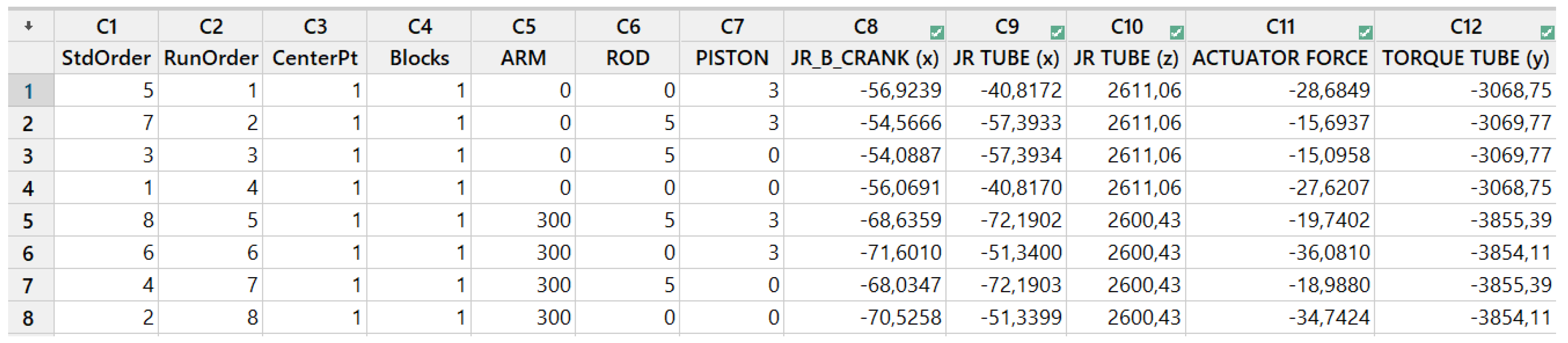
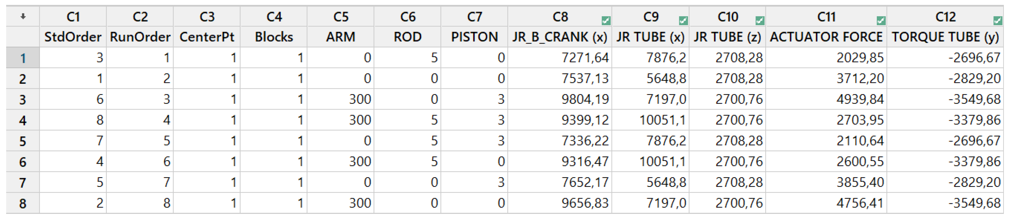
The second phase, after conducting the various simulations according to the elaborated plan of experiments, was to import the data into Excel software to search for the configuration that had higher stresses or active forces and torques to be delivered by the most stressed thrusters, i.e., the points of the structure with the highest constraint reaction and torque. The third step was to import the data into Minitab Statistical Software ver20. and find the optimal configuration by applying the DOE technique. Among the factorial methodologies mentioned above, the one used to conduct this experiment was the full factorial methodology. Specifically, with n, the number of variables to consider is reported, while with m, the number of internal divisions of the variable (base) is defined.

Using the DOE full factorial algorithm, all possible combinations of the variables (given the base) are created so that the number of configurations is $m^n$. In this case, the number of possible combinations was $2^3$ = 8.

This methodology was chosen because it allows for a comprehensive, detailed, precise, and robust analysis of the factors and their interactions, thus offering a deep and comprehensive view of the system. This methodology explores the entire set of variables; therefore, it allows for an exhaustive exploration of each factor and its combinations, checking all possible configurations of the levels of factors that influence the final result and estimating with the highest precision both the main effects of each factor and the interactions between them. In this case, the model is parametric, and the variations are in the order of a few millimeters; consequently, it is essential to ensure high precision and sensitivity in the estimates to estimate best the configuration that offers the most significant benefits. The full factorial approach ensures a more reliable estimation of parameters and a better understanding of phenomena. In addition, it can accurately detect and quantify interactions between factors (this is not possible with other experimental designs such as a fractional factorial design), thus enabling a more detailed analysis of these interactions. Before starting the actual design work, it was essential to identify the main steps to be considered before developing this procedure (see Figure 5).

1.

The identification of the objective: The objective of this analysis was to find the optimal configuration that minimized the constraint reactions and the significant moments acting on the system, which were the output parameters.

2.

The definition of the output parameters: As previously mentioned, the output parameters were the maximum constraint reactions and moments recorded in the system analysis: the actuator force, constraint reaction of the tube (x- and z-axes), constraint reaction of the connecting rod (x-axis), constraint reaction of the crank (x-axis), and tube moment (around the y-axis).

3.

The definition of the input parameters: The independent variables chosen were the arm’s geometric dimensions, the distance between the connecting rod and the uni-ball, and the piston attachment.

4.

Problem modeling: The multibody SimScape R2023b software was used to simulate the system’s behavior under the applied loads and motions.

5.

The optimization of the objective function: The input parameters could take on various values. For the simplification of the testing plan, they were varied between a minimum and maximum value, reported in

Table 2. Levels of factors.

Factor	Min [mm]	Max [mm]	Δ [mm]
ARM	1100	1400	300
ROD	190	193.53	$5cos{45° }^1$
PISTON	311	314	3

¹ The 5 mm increment, considering the connecting rod–uni-ball distance, was multiplied by the cosine of the 45-degree angle, corresponding to the connecting rod’s inclination with respect to the plane.

.

The statistical analysis software Minitab was used to carry out the final phase of the methodology. It provided the values of the specific input parameters needed to ensure the local optimal value of the function’s objective while still adhering to the previously mentioned constraints.

The boundary conditions considered included geometric constraints, kinematic limits, and constraints on the constrained reactions to ensure the physical and numerical validity of the simulations. Introducing these boundary conditions ensured that the Design of Experiments (DOE) generated in Minitab explored only feasible and meaningful configurations, improving the reliability of simulations and facilitating system optimization. One therefore has the following:

1.

Geometric Constraints.

The mechanical system analyzed was subject to length and position constraints, which limited the possible configurations. Specifically, the following constraints applied:

• The dimensions of the arm, rod, and piston components needed to respect relationships that avoid collisions or interference between parts.
• Connections between components needed to adhere to a fixed topology, maintaining minimum clearances to ensure proper assembly.
• The system provided a defined range of motion; configurations that exceeded these limits were not considered in the DOE.

2.

Kinematic Limitations.

The system’s motion was subject to kinematic restrictions to ensure realistic dynamics. Some key aspects included the following:

• Limited angular excursion: The system rotated about the pitch axis in the horizontal flight phase; the angles of rotation could not exceed certain values (e.g., +45°), avoiding unstable configurations.
• Model-compatible velocities and accelerations: The relative motion between components needed to respect limits imposed by the physics of the system, avoiding configurations that generated excessive or impossible accelerations.

The internal and external forces applied to the system needed to remain within acceptable limits to achieve the following:

• Avoid exceeding the structural strength: Component materials were assumed to have load limits; the DOE needed to exclude conditions that generated forces over these values.
• Maintain system stability: Some configurations may have generated reaction forces that were too high in terms of the constraints, causing structural instability or convergence problems in the simulation.

3.

The Physical and Numerical Validity of the Simulations.

For simulations in SimScape to provide reliable results, it was necessary to ensure the following:

• All initial conditions and model parameters were within realistic ranges, avoiding convergence problems.
• The DOE in Minitab excluded experiments with parameters that could lead to computational errors or unphysical results.

Figure 6 and Figure 7 show the experimental plan performed in Minitab.

As mentioned earlier, one of the primary goals of the Design of Experiments (DOE) is to identify the interaction between variables and evaluate their responses. Such an interaction is evaluated by using a linear model with three factors to simulate real-world phenomena influenced by three main parameters while considering the influence of all other factors to be negligible. The mathematical model is reported in (1):

$$y={\beta }_0+{\beta }_1{X}_1+{\beta }_2{X}_2+{\beta }_3{X}_3+{\beta }_{12}{X}_1{X}_2+{\beta }_{13}{X}_1{X}_3+{\beta }_{23}{X}_2{X}_3+{\beta }_{123}{X}_1{X}_2{X}_3+\mathsf{\epsilon }$$

(1)

given the following variables:

• y = the dependent variable, i.e., the value the system response assumes.
• ${\beta }_0$ = the intercept or constant term: represents the expected value y when all independent variables, $X_1$, $X_2$, and $X_3$, are equal to zero.
• ${\beta }_1$, ${\beta }_2$, and ${\beta }_3$ = regression coefficients that measure the effect of each factor (or independent variable) on the dependent variable, i.e., express the interaction between the three independent factors $X_1$, $X_2$, and $X_3$.
  The coefficient of $X_1$ (${\beta }_1$) represents the change in y for one unit change in $X_1$, holding $X_2$ and $X_3$ constant.
  The coefficient of $X_2$ (${\beta }_2$) represents the change in y for one unit of change in $X_2$, holding $X_1$ and $X_3$ constant.
  The coefficient of $X_3$ (${\beta }_3$) represents the change in y for one unit change in $X_3$, holding $X_1$ and $X_2$ constant.
• ${\beta }_{12}$, ${\beta }_{13}$, and ${\beta }_{23}$ = coefficients of the interaction terms between pairs of variables.
  ${\beta }_{12}$$X_1$$X_2$ represents the combined effect of variables $X_1$ and $X_2$ on the dependent variable y. ${\beta }_{12}$ is the coefficient indicating how the effect of $X_1$ on y varies with $X_2$ and vice versa.
  ${\beta }_{13}$$X_1$$X_3$ and ${\beta }_{23}$$X_2$$X_3$ are similar terms describing the combined effect of other pairs of variables.
• ${\beta }_{123}$ = the coefficient of the interaction term between all three variables.
  ${\beta }_{123}$$X_1$$X_2$$X_3$ represents the combined effect of the three independent variables. ${\beta }_{123}$ indicates how the interaction between all three variables, $X_1$$X_2$$X_3$, affects y. This term indicates that the combined effect of all three independent variables is not simply the sum of the effects of each variable and pairwise interactions.
  Interaction effects between three or more factors are often omitted because they are unimportant (negligible influence on the system). However, when they are significant, they can greatly influence the system. Setting two values of $X_1$, $X_2$, and $X_3$ (at the maximum and minimum values), eight experiments were performed, the results of which were used to calculate $eta$ values through linear regression. This highlights the need for thorough analysis in our work.
• $ϵ$ = the experimental error of the mathematical model capturing the variability of y not explained by the independent variables.

The Ordinary Least Squares (OLS) method was used to estimate the parameters ${\beta }_0$, ${\beta }_1$, ${\beta }_2$, and ${\beta }_3$. This method minimizes the sum of the squares of the residuals (the differences between the observed values and the values predicted by the model).

Finally, the model was validated. To validate the model, it was necessary to compare the significance level $\alpha$ with the p-value [20]:

1.

The Definition of the Null Hypothesis $H_0$ and the Alternative $H_1$.

$H_0$ is the null hypothesis, i.e., “no effect”, and is the hypothesis to be tested.

$H_1$ is the alternative hypothesis, i.e., a “significant effect”, and is the hypothesis to be tested.

In this case, hypothesis $H_0$ states that the change in values does not cause a significant effect. In contrast, hypothesis $H_1$, the alternative hypothesis, suggests that changing certain values will result in an optimal configuration by minimizing the constraint reactions, torques, and force to be delivered by the actuator.

2.

Select the significance level $\alpha$.

This is the probability of rejecting the null hypothesis if it is true (first type of error). In this case, $\alpha$ was chosen to be 5%.

3.

Calculating the p-value.

This is the probability of observing a value in the statistical test that is at least as extreme as the observed value, assuming the null hypothesis is true.

4.

The comparison of the p-value and $\alpha$.

If the p-value is ≤$\alpha$, I reject the null hypothesis Ho. There is sufficient evidence to support H1. The probability of observing the data under the null hypothesis is so small that the null hypothesis can be considered unlikely.

If the p-value is ≥$\alpha$, I do not reject the null hypothesis Ho. This means that there is not enough evidence to support the alternative hypothesis H1. The data are not extreme enough to reject the null hypothesis.

3.3. Structural Analysis of Actuation System Using FEM

Finite element analysis is a methodology for solving ordinary partial differential equations concerning engineering and scientific applications. In this study, the FEM technique was used to validate the optimal configuration estimated by the Design of Experiments technique. In particular, in this case study, FEM analysis was used for verifying the DOE results applied to the multibody model. For this purpose, the arm mechanism was modeled with Ansys static to calculate the von Mises stress in correspondence with the actuator’s arm and pin. For the validation of the estimated optimal solutions, a parametric model to test different optimal solutions, if necessary, was even developed. 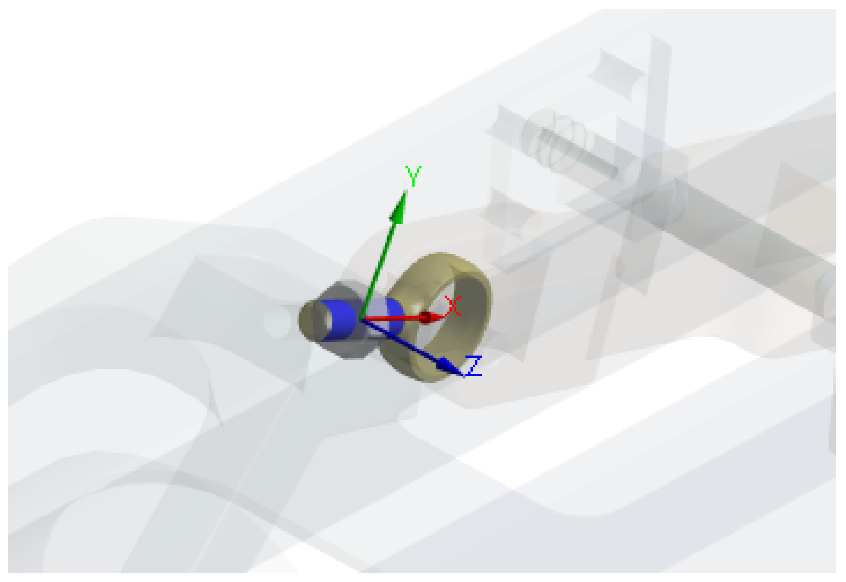Figure 8 shows the translational joint modeled for the 5 mm displacement configuration.

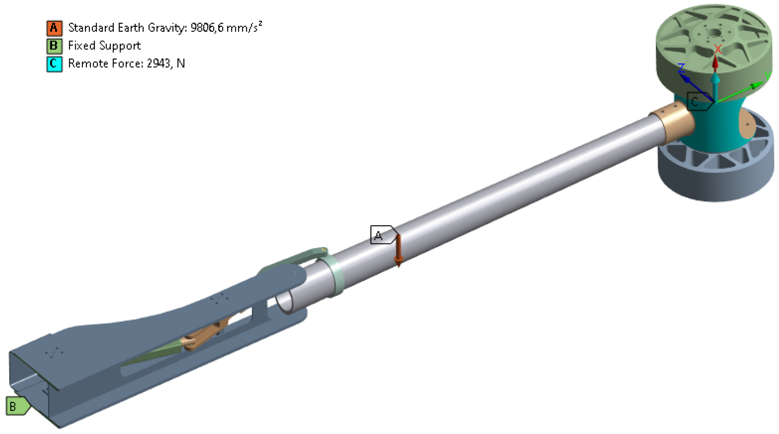
The materials of several components of the mechanism can be seen in Table 1. The software automatically recognized the contacts and defined them as bonded. To ensure the convergence of the analysis, an element size of 1 mm was used for the relevant parts (the actuator and its pin). In detail, the boundary conditions used in the model are shown in Figure 9 where the gravity in the barycenter is shown in orange (letter A); the position of the fixed support is shown in green (letter B) as the structure is schematized as a fixed beam; and the thrust of the motor during take-off is represented in blue (letter C) with a force positioned at the center of mass of the propulsion system.

A statistic analysis was conducted regarding the flight conditions at take-off, where Earth gravity (point A) and the lift force for take-off (point C) were applied on every single arm. For simplicity, the entire vehicle was omitted from the calculation. The opening mechanism was considered blocked for static analysis (point B). The simulation time to consider was set to 1 s with a number of steps equal to one.

4. Results

The analysis with Minitab statistical software revealed that the optimal configuration of the initial project involved a 5 mm increase in the size of the connecting rod. By adjusting the dimensions of the arm, connecting rod, and piston, it was observed that increasing the distance between the connecting rod and the uni-ball by 5 mm optimized the force and torque at critical points compared to the initial configuration. Specifically, the force required decreased by approximately 1700 N at 45 degrees and 13 N for a tilt angle of 0 degrees.

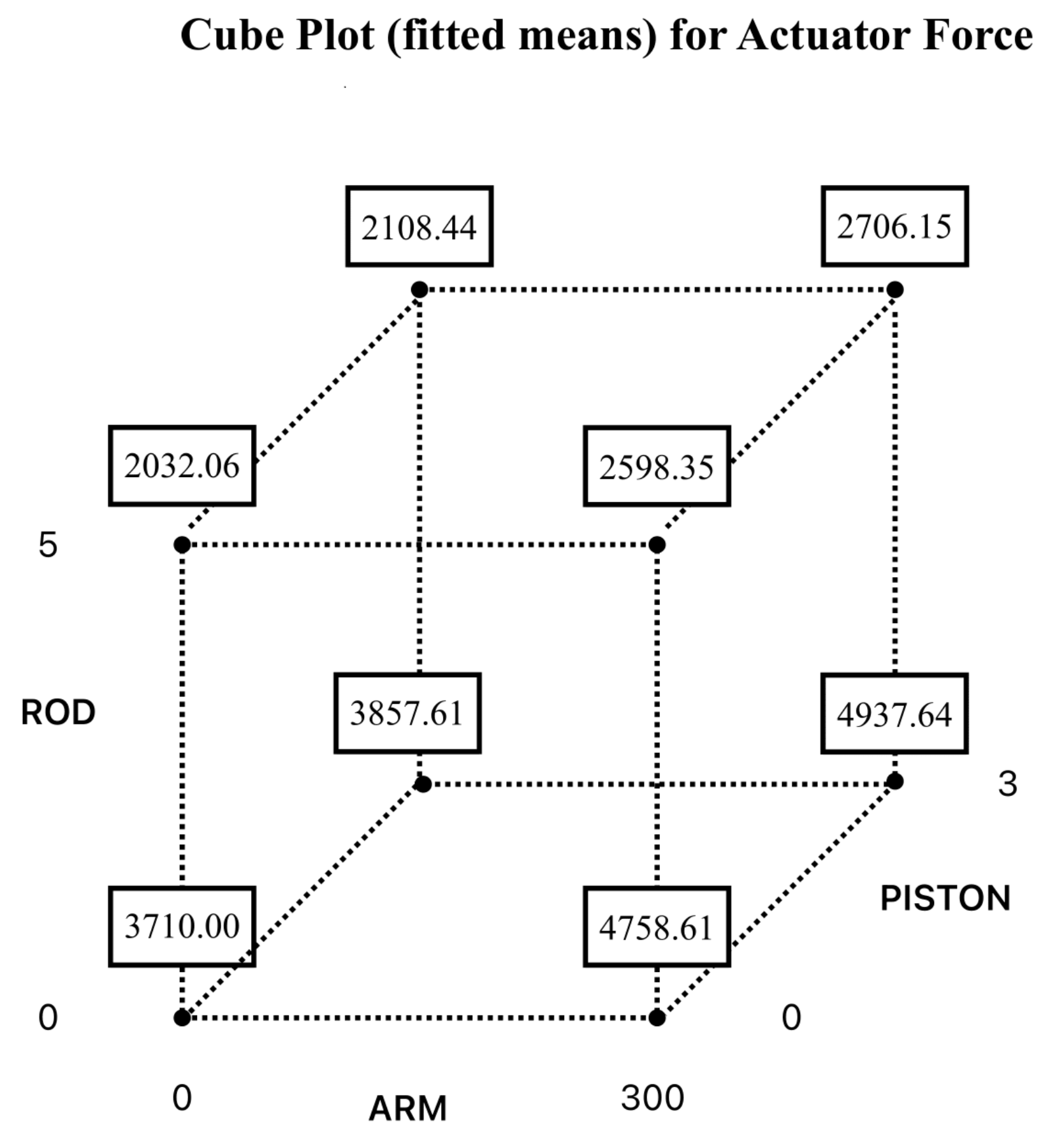
The cube plot in Figure 10 can be used to compare all the tested configurations (obtained by varying important parameters) and, consequently, to evaluate the optimal configuration.

A further comparison can be seen in the histogram in Figure 11, which compares the above configurations according to the percentage of optimization compared to the standard configuration (without the increase in parameter values).

In the

Table 3. Table explaining the histogram data. Δ represents the increase achieved compared to the original measurement.

Configuration	ΔArm [mm]	ΔRod [mm]	ΔPiston [mm]	Optimization [%]
Configuration 1	300	5	3	27.08
Configuration 2	300	5	0	29.98
Configuration 3	300	0	3	−33.03
Configuration 4	300	0	0	−28.20
Configuration 5	0	5	0	45.22
Configuration 6	0	5	3	43.16
Configuration 7	0	0	3	−3.98

, it is possible to observe all configurations related to the histogram and their optimization percentages.

In a Pareto chart, it is possible to observe which components significantly affected the final optimization. In order of magnitude, the graph in Figure 12 shows that these were the connecting rod, arm, arm–rod interaction, and piston; furthermore, the red line represents the level of statistical significance ($\alpha$ = 0.05), and the bars above indicate significant effects. This graph helps to identify key variables for system optimization.

Finally, the results were validated using the p-value and the significance level $\alpha$. The

Table 4. Analysis of variance.

Source	DF	Adj SS	Adj MS	F-Value	p-Value
Model	6	9,148,982	1,524,830	39,261.17	0.004
Linear	3	9,029,635	3,009,878	77,498.02	0.003
ARM	1	1,355,193	1,355,193	34,893.38	0.003
ROD	1	7,641,824	7,641,824	196,760.88	0.001
PISTON	1	32,617	32,617	839.81	0.022
Two−Way Interactions	3	119,347	39,782	1024.31	0.023
ARM × ROD	1	116,317	116,317	2994.92	0.012
ARM × PISTON	1	494	494	12.71	0.174
ROD × PISTON	1	2537	2537	65.31	0.078
Error	1	39	39
Total	7	9,149,021

shows the analysis of variance (ANOVA) used to determine whether there were significant differences between groups in the experiment.

So from table cite, it is possible to obtain the following information:

• DF (Degrees of Freedom): The degrees of freedom indicate the number of independent values that can vary in a statistical analysis. In general, the more degrees of freedom, the more information you have.
• Adj SS (Adjusted Sum of Squares): The adjusted sum of squares represents the variability in the data explained by the model (or by a specific term) after accounting for other terms in the model.
• Adj MS (Adjusted Mean Square): This is the sum of the adjusted squares divided by the degrees of freedom. It indicates the average variance explained by each term in the model.
• F-Value: The F-value is the ratio of the variance explained by the model (or specific term) to the residual variance. A high F-value indicates that the model term explains a significant portion of the variability in the data.
• p-Value: This indicates the probability that the observed results are due to chance. A low p-value (less than 0.05) suggests a significant difference, indicating that the effect is substantial. Model: This row shows the entire statistical model. The associated values show how the entire model behaves concerning the data.
• Linear: This refers to the linear effects of the terms included in the model (arm, rod, piston). It was highly significant, with a p-value of 0.003.
• ARM: The arm-related term significantly affected the outcome, as indicated by the p-value of 0.003 with an F-value of 34,893.38, suggesting that the arm is a significant contributor to the model.
• ROD: The term related to the rod had a highly significant effect with a p-value of 0.001 and with an even higher F-value (196,760.88), suggesting a strong influence.
• PISTON: The term related to the piston had a significant effect with a p-value of 0.022, but its effect was smaller than that of the arm and rod, as indicated by the lower F-value (839.81).
• Two-Way Interactions: These refer to the interactions between two terms (factors). These interactions show how the combined effect of two factors may differ from the effect of each factor considered separately.

  -

  ARM × ROD: The interaction between the arm and rod was significant (p-value of 0.012).

  -

  ARM × PISTON: The interaction between the arm and piston was not significant (p-value of 0.174).

  -

  ROD × PISTON: This interactive effect was borderline (p-value = 0.078), so it might have had a slight impact, but it was not significant.

• Error: This row represents the variation not explained by the model, attributable to random errors. The sum of squares of the error (39) was very low, which means that most of the variation was explained by the model.

The table shows that the overall model was significant (p-value = 0.004), with important effects for the linear terms arm, rod, and piston. Among the interactions, the ARM × ROD interaction was substantial, while ARM × PISTON was not. The ROD × PISTON interaction was marginally non-significant. This table is typical of a study in which several factors and their interactions are evaluated to see how they influence a measured response. The results suggest that both individual factors and some of their interactions had a significant effect on the response variable.

The additional verification of the solution selected as optimal was obtained by subjecting all configurations to two further cases always evaluated at angles, $\theta$, of 0 deg and 45 deg, i.e., in the case of a malfunction with the incomplete opening of the arm ($\alpha$ = 30 deg) and the case of operation under normal conditions with the application of an orthogonal force equal to 2943 N. Even under these conditions, the solution selected in the previous analysis proved to be the optimal solution.

FEM analysis, combined with DOE techniques and the MBD approach, could be employed to validate the predicted optimal solutions. This application used static analysis to evaluate the actuator’s arm and pin behavior for the optimal solution that minimizes the linear actuator’s active force during hovering. Minimizing the actuator force will allow for the reduction of energy consumption during flight operation.

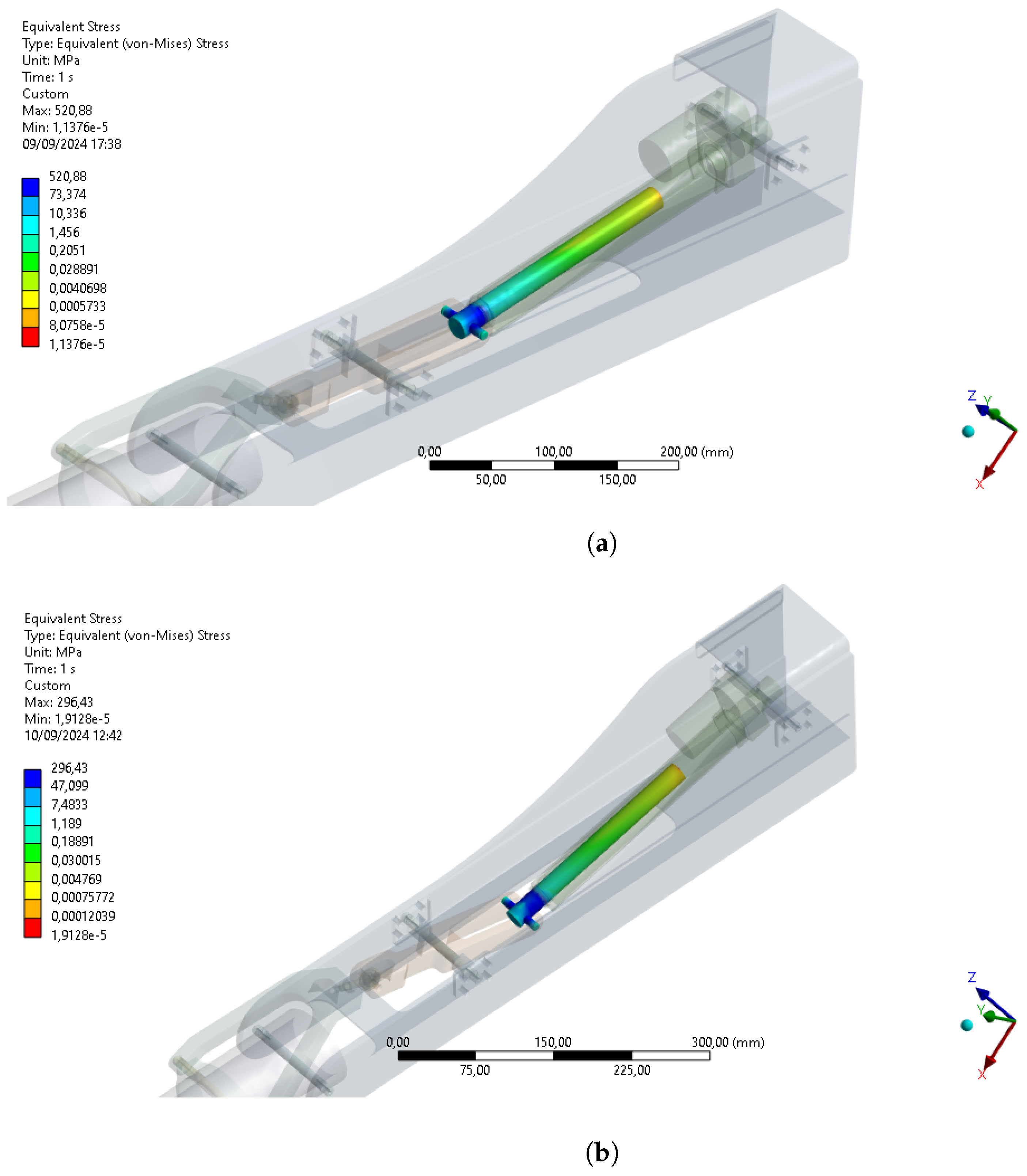
Figure 13 shows, as an example, the equivalent von Mises stress on the pin of the linear actuator for a non-optimized configuration (see Figure 13a) and optimized configuration (see Figure 13b).

In the non-optimized configuration, the maximum stress reached 520.88 MPa, whereas in the optimized configuration, it was reduced to 296.43 MPa.

5. Discussion

The analyses conducted allowed the initial concept to be validated through the application of DOE techniques, but more importantly, they allowed the optimal configuration of the structure to be identified. Specifically, the optimization achieved by a 5 mm increase in the size of the connecting rod resulted in a significant reduction in the actuator force, with a decrease of about 1700 N for an angle of 45 deg and 13 N for an angle of 0 deg.

Pareto diagram analysis showed that the most influential factors in force optimization are the connecting rod, the arm, their interaction, and the piston. This shows that optimizing these components can significantly improve the efficiency of the mechanical system by reducing operating loads. In addition, the histogram showed that the most effective configuration achieved up to 45.22 percent force optimization compared with the initial configuration.

The results of the ANOVA confirmed the statistical significance of these optimizations: the connecting rod (p-value = 0.001) and arm (p-value = 0.003) emerged as the most critical parameters, while the interaction between the arm and connecting rod showed a significant impact (p-value = 0.012). Compared with the standard configuration, the optimized solution resulted in a significant reduction in the stress on critical components. In particular, FEM analysis confirmed that the maximum von Mises stress on the pin was reduced by about 224.45 MPa, suggesting a potential increase in the component life and reliability. These results have direct practical implications in mechanical system design, especially in applications where energy efficiency and durability are critical factors. Reducing the force required from the actuator could allow for lower energy consumption, extending the component life and improving the overall system reliability.

Despite the promising results, some limitations need to be recognized. Future studies should focus on analyzing and validating these results through dynamic flight models and experimental testing, so as to verify their applicability in real-world scenarios and the robustness of the optimized configuration under varying load conditions. In addition, material properties and manufacturing tolerances were not considered in this study, factors that could affect the performance of the system in the real world. In summary, this study demonstrated how small geometrical changes can lead to significant improvements in actuator efficiency by reducing both the required force and structural stress. The findings provide a solid basis for further research on optimization strategies for mechanical joints, with possible applications in aerospace, robotics, and industrial automation.

Moreover, from a future perspective, the implementation of diverse optimization algorithms could be evaluated to compare innovative methodologies and identify the most efficient system. This approach could optimize research efforts and further reduce associated costs, helping to overcome the critical issues still present in urban air mobility and promote the development of this emerging technology.

6. Conclusions

In recent years, the expansion of urban areas and the increase in road co-management in cities have led the effort-driven world to explore innovative solutions to optimize mobility. In this scenario, urban air mobility (UAM) has emerged as one of the most promising technologies [21]. It has the potential to radically transform transportation in urban areas, contributing to creating a more sustainable and interconnected transportation system.

The origins of UAM can be traced back to the use of light aircraft and drones for emergency operations, such as transporting patients and medical supplies to areas that are difficult to reach from the ground, but with the advancement of technologies, particularly in the areas of electric propulsion and vertical take-off and landing (eVTOL) systems, the interest in air mobility has expanded beyond just emergency applications. Today, UAM presents a challenge to improve mobility to integrate air transport in large cities, improve connectivity, reduce pollution, and optimize the use of urban space.

According to United Nations forecasts, by 2050 about 68% of the world’s population will live in urban areas, further increasing the demand for efficient and environmentally friendly transportation infrastructure [22]. In this context, UAM presents an opportunity to alleviate pressures on land infrastructure by reducing the travel time and improving connectivity within cities.

In the context of the growing adoption of UAM vehicles, this work aimed to develop, through combining multibody simulations and Design of Experiments techniques, a methodology for guiding a designer during the preliminary design phases. This is a method of searching for the optimal configuration that minimizes the constraint reactions and torques acting on the system at the most stressed points and the force delivered by the actuator. The ultimate goal is to obtain an optimized system that reduces costs, consumption, and the forces developed while ensuring efficiency, effectiveness, and compliance with technical specifications and safety standards.

Currently, the major critical issues in UAM are as follows [23,24]:

1.

Costs for their design, implementation, and development;

2.

Security;

3.

Autonomy and battery life;

4.

Emissions from battery production and disposal;

5.

Sustainability, specifically regarding the energy production and consumption needed to recharge vehicles.

Using the DOE methodology, it was possible to reduce the number of design attempts. Thanks to the software, a direct comparison of potential solutions was made, allowing for a drastic reduction in the time taken and costs related to the development and implementation of solutions, as well as the search for the optimal solution. In addition, the feasibility and compliance with preestablished security criteria were verified. The analyses conducted using the different software ensured structural safety in all phases of flight: the obtained solution allows the structure to optimally handle stresses, without exceeding a certain weight. The present study allowed for a significant reduction in the constraint reactions and torques acting on the system, thus reducing the stress at the points defined as critical in the standard solution and the work required by the actuator. The relative advantages are shown below:

1.

Increased energy efficiency and a reduced system energy footprint: The load that the actuator has to carry and the external forces decrease; as a result, I have achieved a reduction in the total energy consumption.

2.

Reduced friction and losses: Unnecessary losses are minimized; as a result, the battery can provide energy for a longer time with a lower charging frequency.

3.

Increased battery life: There is a reduction in the amount of energy required for operation; therefore, I have extend the battery’s charge life, and it is used more efficiently.

4.

Reduction in thermal overload: The mechanical system becomes more efficient, and as a result, it produces less heat. Heat can reduce the efficiency of the battery; therefore, the battery life is prolonged.

Through these analyses, it was possible to identify and address all the disadvantages associated with this innovative solution. It is a more sustainable solution because it reduces the energy consumption for battery charging, increases the battery range and battery life, and helps reduce the frequency of battery production and disposal. In summary, reducing the torque and binding reactions makes the system more efficient and effective, reduces the costs associated with it, and at the same time, there is a positive environmental impact.