The Fault Diagnosis of Rolling Bearings Based on FFT-SE-TCN-SVM

Abstract

Traditional fault diagnosis methods often require extracting features from raw vibration signals based on prior knowledge, which are then input into intelligent classifiers for pattern recognition. This process is prone to information loss and can be inaccurate when relying on human experience for fault identification. To address this issue, this paper proposes an intelligent fault classification and diagnosis model for rolling bearings based on Fast Fourier Transform (FFT) combined with a time convolutional network (SE-TCN) incorporating an attention mechanism, with a Support Vector Machine (SVM) used as the classifier. First, the FFT is applied to transform the collected raw time-domain data of bearing faults into the frequency domain, obtaining the sequence information in the frequency domain. Second, the frequency–domain sequence data are fed into the SE-TCN model, which uses multiple convolutional layers and a channel attention mechanism to extract deep fault features. Finally, the extracted feature vectors are input into the SVM classifier, and the Particle Swarm Optimization (PSO) algorithm is used to optimize the SVM parameters. The optimal separating hyperplane is obtained through training to classify the fault types of the rolling bearings. To verify the effectiveness and diagnostic performance of the proposed method, experiments are conducted using bearing fault datasets from Case Western Reserve University (CWRU) and a laboratory self-built fault diagnosis experimental platform. The experimental results show that the classification accuracy of the proposed method exceeds 99% on the CWRU test dataset, and it also demonstrates advantages in handling small sample data, with an accuracy of over 90%. Additionally, it exhibits good diagnostic performance on the bearing fault data collected from the laboratory self-built platform. The results validate the effectiveness of the proposed classification model in bearing a fault diagnosis.

1. Introduction

Bearings, as critical components in rotating machinery, play a crucial role in determining the performance and reliability of the entire mechanical system [1,2,3]. In practical industrial applications, due to various factors such as design, manufacturing, installation, and operating conditions, bearings are among the most prone components to failure [4]. Therefore, timely diagnosis of bearing faults is essential for the overall safety and efficient operation of the equipment [5].

Vibration signal-based analysis is the most commonly used and reliable method for rolling bearing fault diagnosis [6,7,8]. This method combines signal decomposition techniques with envelope analysis to reduce noise and extract fault characteristic frequencies. These extracted frequencies are then compared with the theoretical fault characteristic frequencies of different bearing components, allowing for the identification of faults at various positions within the bearing. In reference [9], linear frequency cepstral coefficients are introduced as features from vibration sensor data to enhance the performance of rolling bearing anomaly detection. Reference [10] proposes a novel sparse time–frequency analysis method that integrates the frequency adaptability of the S-transform and the iterative computation of the multi-synchronous compression algorithm, overcoming the limitations of the fixed sliding window in short-time Fourier transform. This approach enables a time–frequency representation with higher energy concentration. However, when diagnosing faults through bearing vibration signal analysis, manual expertise is required for feature extraction, leading to lower diagnostic efficiency. Additionally, this method demands that the operator possess certain professional knowledge and a good understanding of the bearing’s structural parameters [11].

Fault diagnosis is essentially a pattern recognition process, and shallow machine learning methods are typical approaches for pattern recognition [12,13]. By combining fault feature extraction with shallow machine learning methods, signal denoising and fault feature extraction are first performed using time-domain, frequency–domain, and time–frequency domain signal processing techniques. The extracted features are then input into shallow machine learning algorithms for fault classification. Reference [14] proposes a bearing fault diagnosis model based on the Circular Entropy Spectrum (CCES) and Least Squares Support Vector Machine (LSSVM) under impulse noise conditions. First, CCES is used to extract narrowband kurtosis vector features, which are then classified using the LSSVM model. This model demonstrates good experimental results and exhibits strong adaptive capability. Furthermore, Reference [15] introduces a model that combines artificial neural networks with dimensional analysis for bearing fault size diagnosis. The results show that the diagnostic efficiency of the artificial neural network outperforms dimensional analysis, with the error band performance and actual error being approximately 97.79% and 5.49%, respectively. This highlights the performance of artificial neural networks and the simplicity of data preprocessing. However, due to the shallow structure typically used in machine learning algorithms, their ability to extract nonlinear features from complex datasets is limited, and they heavily rely on carefully selected fault features [16].

Deep learning methods have been widely applied in bearing fault diagnosis due to their ability to automatically extract features and uncover hidden nonlinear relationships within large datasets [17,18]. Reference [19] aims to enhance the accuracy of rolling bearing fault recognition by utilizing cyclic spectral analysis to estimate the two-dimensional cyclic spectral coherence diagram of vibration signals, thereby generating bearing classification patterns that can distinguish different fault types. Reference [20] investigates three time–frequency transformation methods—Short-Time Fourier Transform (STFT), Continuous Wavelet Transform (CWT), and S-transform—for converting one-dimensional vibration signals into two-dimensional time–frequency images, and their application in convolutional neural network (CNN)-based rolling bearing fault diagnosis. Reference [21] proposes a bearing fault diagnosis method based on spectral image information fusion and CNN. This method analyzes multi-channel vibration signals using STFT to obtain frequency–domain information, which is then fused into two-dimensional images and input into a CNN for training, resulting in a fault diagnosis model. The model’s diagnostic performance is validated using an existing dataset to achieve intelligent and efficient fault diagnosis. Reference [22] introduces a multi-scale recursive fusion strategy guided by an attention mechanism. This strategy effectively allocates attention, allowing deep neural networks (DNNs) to focus more on useful information in adjacent layers, thereby accurately representing potential features related to changes in working conditions.

Although deep learning methods have achieved good diagnostic results in the aforementioned literature, there are still limitations in addressing time series data. When handling sequential tasks, Recurrent Neural Networks (RNNs) are more effective but are prone to issues such as vanishing or exploding gradients. To address this problem, Reference [23] proposes a data-driven bearing performance degradation assessment method based on Long Short-Term Memory Recurrent Neural Networks (LSTM-RNNs), which improves the ability to handle long-term dependencies, a common limitation in traditional RNNs. Reference [24] introduces a deep learning framework combining LSTM-RNN, Stacked Autoencoders (SAEs), and Particle Swarm Optimization (PSO), focusing on fault detection by utilizing unlabeled historical data and unknown abnormal features.

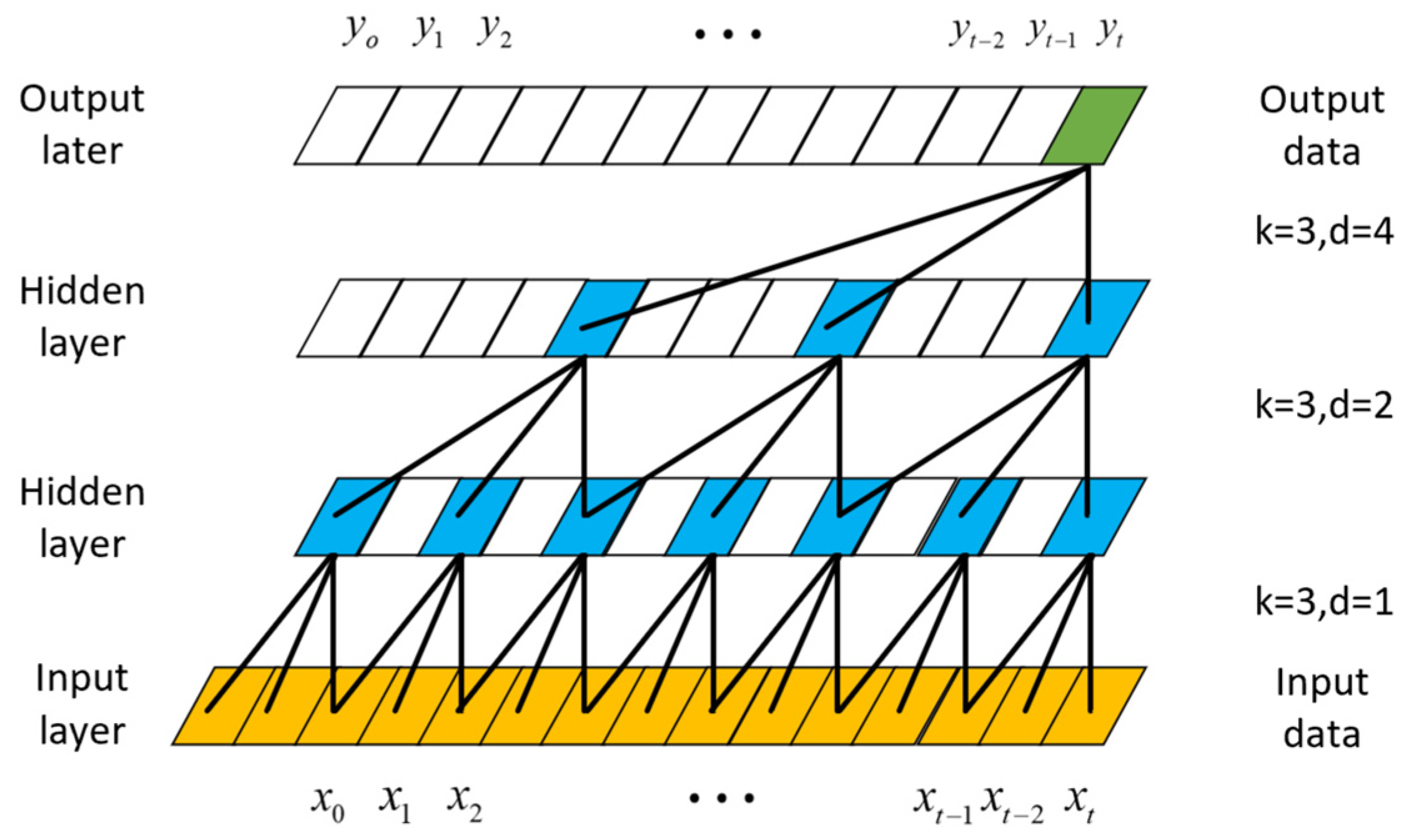
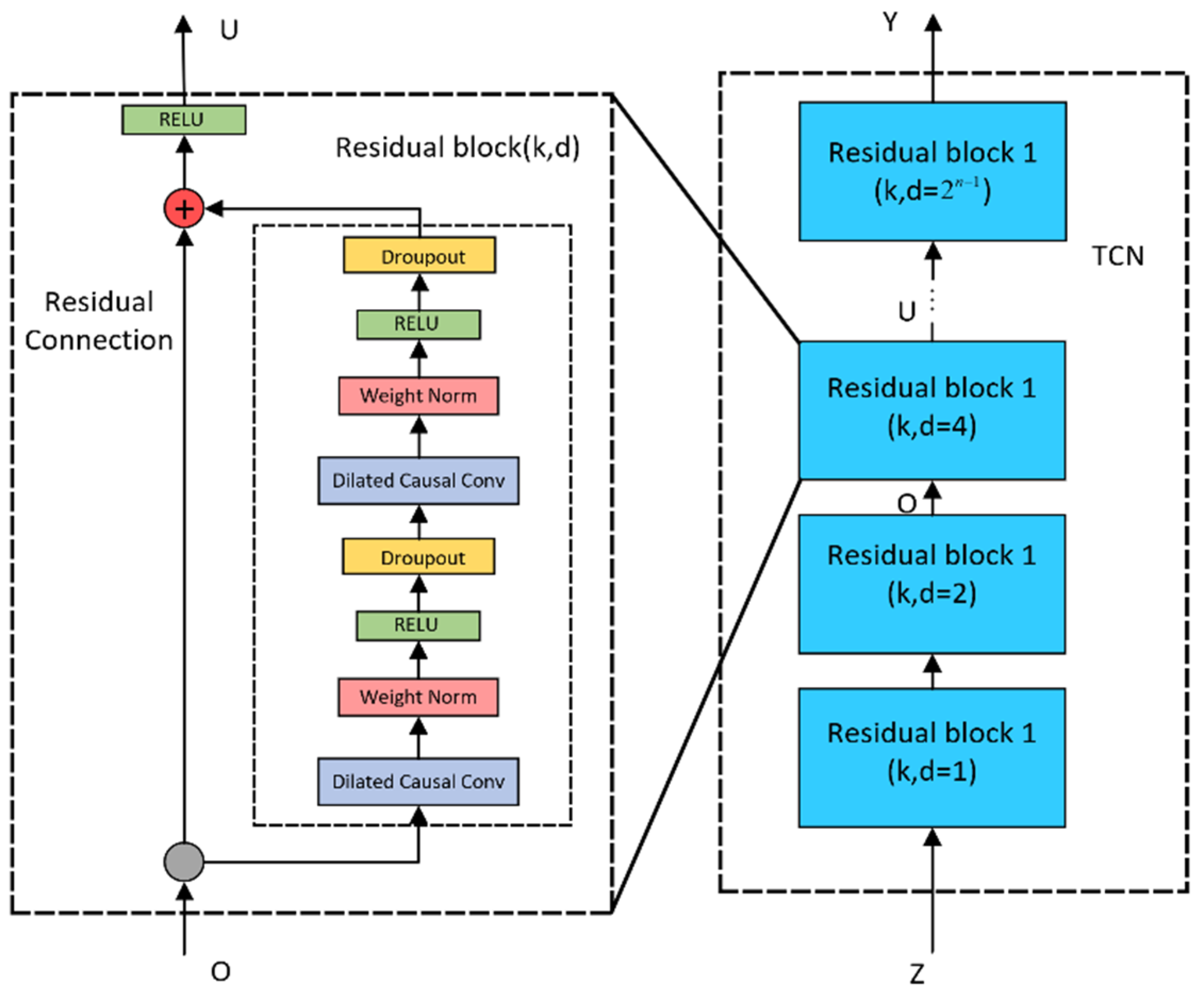
In recent years, Temporal Convolutional Networks (TCNs) have been shown to outperform CNNs and LSTMs in handling sequence data problems [25], and significant progress has been made in fault diagnosis research. Reference [26] combines TCN with an attention mechanism for remaining useful life (RUL) prediction of rolling bearings, demonstrating that TCN is effective in predicting vibration trends and RUL for rolling bearings. Reference [27] proposes a bearing fault diagnosis model based on an attention-based Temporal Convolutional Network and Bidirectional Gated Recurrent Units (Bi-GRU), with results indicating that this method outperforms 1D Convolutional Neural Networks, Bidirectional Long Short-Term Memory Networks, and Bidirectional Recurrent Neural Networks in terms of identification accuracy. Numerous studies have shown that TCN, with its simple convolutional architecture, performs better than classical recurrent networks across different tasks and datasets. Moreover, TCNs offer advantages such as large effective memory, parallelizable convolution, flexible receptive fields, and stable gradients.

Traditional Temporal Convolutional Networks (TCNs) for fault diagnosis typically use a Softmax classifier for fault classification. Although the Softmax classifier effectively integrates with the network during the training phase and facilitates weight updates for the TCN model, it has several drawbacks, including poor performance on nonlinear problems, insufficient model generalization, a large number of parameters that increase computational time, and susceptibility to overfitting. On the other hand, Support Vector Machines (SVMs) perform well in handling small sample sizes and nonlinear issues [28], with stronger generalization capabilities. Therefore, this paper replaces the fully connected Softmax classifier with an SVM.

The Fast Fourier Transform (FFT) is an efficient algorithm used to compute the Discrete Fourier Transform (DFT) and its inverse transform [29]. In signal processing, by exploiting symmetry and periodicity, a set of data with a time duration of T can be transformed into a T/2-point DFT, which is then further reduced to T/4-point, T/8-point DFTs, and so on, significantly reducing the computational load. As the number of FFT points increases, the computation speed approaches linear growth, making FFT highly efficient for period calculations. In rolling bearing fault diagnosis, FFT can convert time-domain signals into frequency–domain signals, enabling the extraction of fault characteristic frequencies and their harmonics. The advantage of this method lies in its ability to effectively reduce noise interference, highlight fault features, and provide clearer data support for subsequent feature extraction and classification [30].

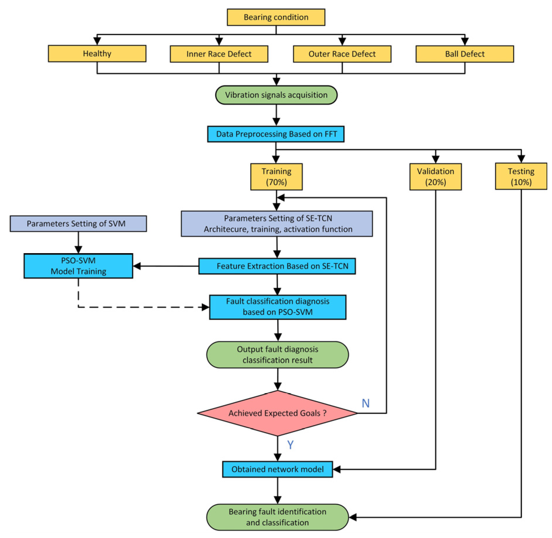
In order to fully leverage the advantages of different models, this paper proposes a rolling bearing fault diagnosis method that combines Fast Fourier Transform (FFT), a Time Convolutional Network (TCN) with an integrated attention mechanism (SE-TCN), and Support Vector Machine (SVM) (hereinafter referred to as FFT-SE-TCN-SVM). The basic idea is as follows:

(1)

Use FFT as a preprocessing step for the bearing fault vibration signal to reduce dimensionality and denoise the original signal, highlighting the key frequency components. This makes it easier for the TCN to capture the critical features, thereby improving diagnostic accuracy;

(2)

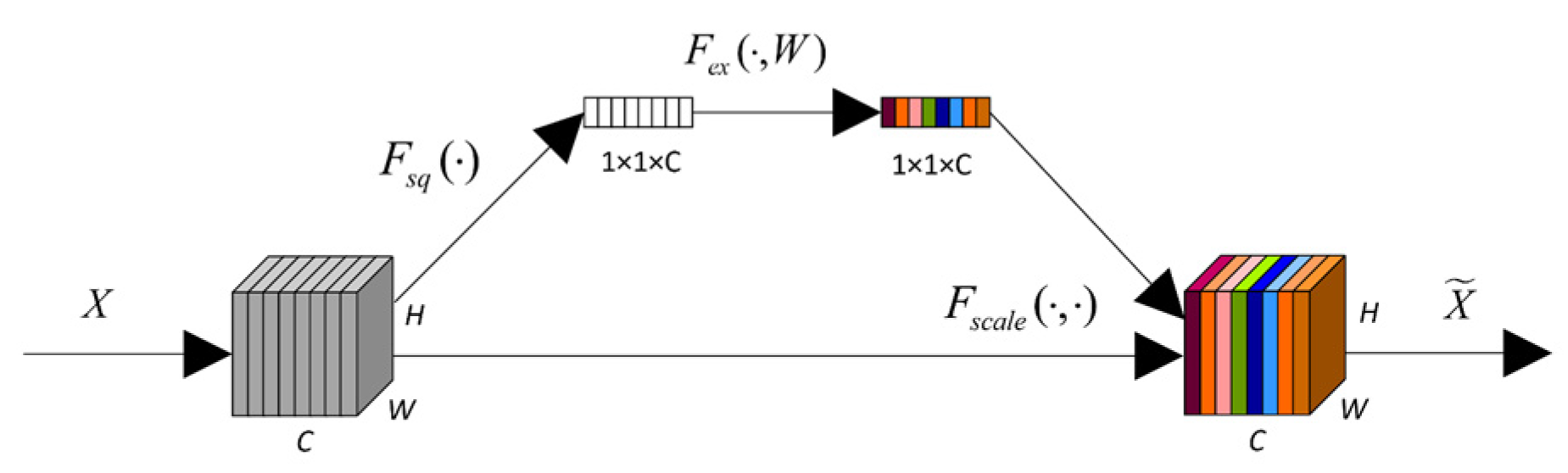
Process the data using the TCN model and enhance it with the attention mechanism from SENet to improve the feature extraction capability of the TCN network. This enables the model to selectively focus on channels with key information, especially in regions where the signal shape undergoes significant changes, thus strengthening the model’s feature representation ability;

(3)

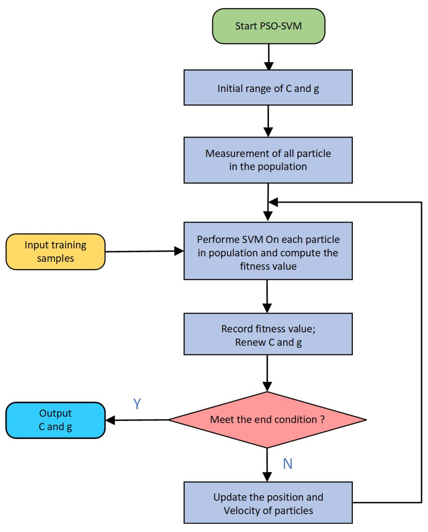
Replace the original Softmax classifier with a classic SVM classifier and optimize the parameters using Particle Swarm Optimization (PSO) to further improve the classification capability of the network.

The structure of the article is as follows: Section 2 introduces the principles of FFT, SE-TCN network, and SVM, and provides a detailed description of the flowchart of the proposed method. Section 3 conducts a case study using the CWRU and laboratory-collected bearing fault datasets to validate the effectiveness of the proposed method. Finally, Section 4 offers the concluding remarks of the paper.

2. Principle of FFT-SE-TCN-SVM

2.1. Signal Preprocessing Based on the Fast Fourier Transform (FFT)

During the operation of mechanical equipment, the motion behavior of the bearing reflects the dynamic changes in the condition of the components. When a bearing fails, this information changes and can be extracted through monitoring technologies such as vibration and acoustic emission. Different types of faults typically have relatively stable characteristic frequencies. However, the extracted signals are usually represented in the form of time-domain waveforms, which are not effective in providing the information needed for fault diagnosis and make it difficult to accurately locate the fault. By applying FFT, the time-domain signal can be transformed into frequency–domain feature sequence data, providing more effective data support for the next stage of TCN processing.

FFT is an efficient algorithm for computing the Fourier transform, enabling the transformation of a signal from the time domain to the frequency domain. The basic idea is to exploit the periodicity and symmetry of the sequence, decomposing the discrete Fourier transform (DFT) of a long sequence into the sum of DFTs of multiple shorter sequences [31,32].

For a sequence $x\left(n\right)$ of length $N$, the formula for the discrete Fourier transform is

$$\begin{array}{l}X(n)={\displaystyle \sum _{k=0}^{N-1}x(k){W_N}^{nk}},n=0,1,2,\cdots ,N-1\\ x(k)={\displaystyle \frac{1}{N}}{\displaystyle \sum _{n=0}^{N-1}X(n){W_N}^{-nk}},k=0,1,2,\cdots ,N-1\end{array}$$

(1)

In the formula, $W_N=e^{-j2\pi /N}$ is the rotation factor, $x\left(n\right)$ represents the sampled values of the waveform signal, $N$ is the number of sequence points, $n$ is the index of the discrete values in the frequency domain, and $k$ is the index of the discrete values in the time domain.

By dividing the sequence $x\left(n\right)$ into two groups, the expression for the DFT of two sequences, each of length $N/2$, can be derived as follows:

$$X(n)=DFT\left[x(2u)\right]+DFT\left[x(2u+1)\right]={\displaystyle \sum _{u=0}^{N/2-1}{x}_1(u){W_{N/2}}^{uk}+{W_N}^k{\displaystyle \sum _{u=0}^{N/2-1}{x}_2(u){W_{N/2}}^{uk}}},u=0,1,\cdots ,N/2-1$$

(2)

When N is large, performing the DFT on the two sequences after a single decomposition is relatively complex. To simplify the computation, the sequence can be recursively decomposed, and the results of the smaller DFTs are then used to reconstruct the DFT of the original signal. This decomposition approach significantly reduces the computational workload. The time complexity of the traditional DFT algorithm is $o\left(N^2\right)$, while the time complexity of the FFT algorithm is only $o\left(NlogN\right)$.

The Fourier expansion of the signal $x\left(t\right)$ is given by

$$x(t)={\displaystyle \frac{a_0}{2}}+{\displaystyle \sum _{n=1}^{\infty }\left[a_n\cos (2\pi n{f}_{1}t)+b_n\sin (2\pi n{f}_{1}t)\right]}$$

(3)

In the formula, $a_n$ and $b_n$ are the Fourier coefficients, which are given by

$$\begin{array}{l}{a}_n={\displaystyle \frac{2}{T}}{\displaystyle {\int }_0^{T}x(t)}\cos (2\pi n{f}_{1}t)dt\\ b_n={\displaystyle \frac{2}{T}}{\displaystyle {\int }_0^{T}x(t)}\sin (2\pi n{f}_{1}t)dt\end{array}$$

(4)

2.2. Feature Extraction Based on the Attention Mechanism Temporal Convolutional Network (SE-TCN)

2.2.1. Temporal Convolutional Network (TCN)

The Temporal Convolutional Network (TCN) [33] is a variant of convolutional neural networks (CNNs) designed for sequential tasks. It not only inherits the advantages of CNNs in processing long time sequences but also avoids the gradient explosion problem that is commonly encountered in Recurrent Neural Networks (RNNs) and Long Short-Term Memory Networks (LSTMs). The core idea is to build upon CNNs by introducing causal convolutions and dilated convolutions and using residual connections to effectively enhance the network’s ability to process temporal sequence information [34].

• Causal Convolution

Causal convolution employs a unidirectional structure, ensuring that when processing long time series data, the output and input have the same length through a one-dimensional architecture. This maintains a one-to-one correspondence between the sequence data, preserving the causal relationship. Therefore, the value at time t depends only on the information from the previous time step and the data up to time t, but not on any future information.

Assuming the convolutional kernel is set as $F=(f_1,f_2,\cdots ,f_k)$ and the input time series is $X=(x_1,x_2,\cdots ,x_t)$, the causal convolution at $x\left(t\right)$ can be expressed as

$${(F\ast X)}_{(x_t)}={\displaystyle \sum _{k=1}^K{f}_k·x_{t-K+k}}$$

(5)

In the equation, $\ast$ denotes the convolution operation.

2.

Dilated Convolution

Dilated convolution applies interval sampling during the convolution process, enabling the capture of long-term sequence dependencies and corresponding relationships. The dilation factor d determines the spacing between adjacent data points in the input layer during computation, affecting the sampling rate and the receptive field of the Temporal Convolutional Network (TCN).

While causal convolution enhances feature learning capabilities, the length of long-term sequences cannot be excessively long due to the increased number of layers. Therefore, dilated convolution is introduced to address this limitation. As shown in Figure 1, with the increase in the number of hidden layers, the dilation factor increases exponentially. A relatively small number of layers is sufficient to achieve a larger receptive field.

3.

Residual Connection

The principle of residual connections lies in learning the identity mapping function, enabling the network model to propagate information across layers. By adding residual modules between the layers of the network model, the training process is simplified, and the classification accuracy is effectively improved.

Suppose the input to the residual module is $X$ and the identity mapping function $F\left(X\right)$ exists across the layers. The final result is added to $X$, and the output $P$ can be expressed as

$$P=Acticvation(X+F(X\left)\right)$$

(6)

Figure 2 shows the structure of the TCN residual block. In the TCN model, residual connections are typically composed of multiple modules connected in series. Each residual module consists of two layers of causal dilated convolutions, and the nonlinear mapping function is implemented using the ReLU activation function. The residual connections normalize the weights for the convolutional kernels and add a dropout layer after each causal dilated convolution to effectively prevent both underfitting and overfitting.

Since TCN employs causal convolutions to prevent the loss of information when processing complex time series and dilated convolutions are used to handle complex sequence information, the incorporation of residual modules simplifies the network model’s training. Therefore, TCN has certain advantages in processing rolling bearing fault signals.

2.2.2. Attention Mechanism

In the process of feature extraction, the TCN (Temporal Convolutional Network) assumes that each feature channel has the same importance. However, in practical applications, the impact of different feature channels on the target parameter varies, resulting in the TCN’s inability to accurately allocate the contribution of each feature channel. This imbalance affects the accuracy of bearing fault classification.

SENet can address this issue by adaptively adjusting the importance of feature channels. It allows the network to focus on more effective features, thereby improving the accuracy of fault classification [35,36]. The SE (Squeeze-and-Excitation) module, as an attention mechanism, primarily involves three steps: Squeeze, Excitation, and Scale. Figure 3 shows the structure of the SENet model.

• Sequeeze

The Squeeze operation compresses the feature map of size H × W × C, which contains global information, into a $1\times 1\times C$. feature vector through global average pooling. This feature vector has a global receptive field. The mathematical expression is as follows:

$$z_c=F_{sq}(x_c)={\displaystyle \frac{1}{H·W}}{\displaystyle \sum _{i=1}^H{\displaystyle \sum _{j=1}^W{X}_c(i,j)}}$$

(7)

In the equation, H and W represent the height and width of the feature map, respectively; C is the number of channels; and z_c is the weight generated by the Squeeze operation.

2.

Excitation

The Excitation operation extracts the correlation between feature channels through two fully connected layers.

The first fully connected layer performs dimensionality reduction, containing $C/r$ neurons, with an input dimension of $1\times 1\times C$ and an output dimension of $1\times 1\times C/r$. Here, $r$ is a scaling parameter, designed to reduce the number of channels, thereby lowering the computational cost and enhancing the model’s generalization ability. The second fully connected layer restores the original dimension, containing $C$ neurons, with an input dimension of $1\times 1\times C/r$ and an output dimension of $1\times 1\times C$.

The mathematical expression is as follows:

$$S_c=F_{ex}(z_c,W)=\sigma \left[W_2\delta (W_1{z}_c)\right]$$

(8)

In the equation, $\delta$ represents the ReLU function, σ represents the Sigmoid function, and $W_1$ and $W_2$ are the matrix parameters to be learned for capturing the feature correlation between channels.

3.

Scale

Finally, the weight adjustment operation multiplies the original features by the learned channel weights, adjusting the feature map output from the excitation operation to match the dimensions of the original features, changing the dimensions from $1\times 1\times C$ to $H\times W\times C$.

The mathematical expression is as follows:

$$\widetilde{X_c}=F_{scale}(X_c,S_c)=S_c\otimes X_c$$

(9)

In the equation, $\otimes$ represents element-wise multiplication.

Figure 4 shows the structure of the SE-TCN residual block. Each SE-TCN residual block contains two dilated causal convolution layers with dilation rates of d = 1 or d = 2. The two convolution layers within the same residual block share the dilation rate, making the model parameters more compact and allowing it to capture similar temporal features at different time steps. The dilation rates of different residual blocks grow exponentially, enabling the network to gradually expand its receptive field as the layers increase, thus effectively capturing long-range dependencies. SE-TCN, by combining dilated causal convolutions and SE modules, can efficiently capture dependencies at different time scales when processing time-series data, while the residual block structure enhances the flow of information, improving the model’s performance.

2.3. Fault Classification Diagnosis Based on the Particle Swarm Optimization Support Vector Machine (SVM)

2.3.1. Support Vector Machine

The Support Vector Machine (SVM) is a machine learning algorithm based on statistical theory, which is suitable for solving small sample classification problems. It has been widely used for non-linear, small sample, and high-dimensional pattern recognition [37]. In practical applications, rolling bearings often suffer from insufficient data collection, making it difficult to gather fault samples, resulting in a limited number of samples. Therefore, SVM is commonly used for fault diagnosis of rolling bearings.

The basic principle of SVM is to map nonlinear problems in the original low-dimensional input space to a high-dimensional feature space for solving.

The optimal function can be obtained as

$$f(x)=\mathrm{sgn}({\displaystyle \sum _{i=1}^N{{\alpha }_i}^{\ast }{y}_{i}K(x_i,x)}+b^{\ast })$$

(10)

Common kernel functions include the linear kernel, polynomial kernel, radial basis function (RBF) kernel, and sigmoid kernel. For nonlinear classification problems, the radial basis function (RBF) has advantages such as the ability to map samples to higher-dimensional spaces nonlinearly and fewer constraints on numerical conditions. Therefore, the kernel function selected in this paper is the RBF kernel, and its expression is as follows:

$$K(x_i,x)=\exp (-\gamma {‖x-x_i‖}^2),\gamma ={\displaystyle \frac{1}{2g^2}}$$

(11)

The final decision classification function is

$$f(x)=\mathrm{sgn}({\displaystyle \sum _{i=1}^N{{\alpha }_i}^{\ast }{y}_i\exp (-\frac{{‖x-x_i‖}^2}{2g^2})}+b^{\ast })$$

(12)

In the equation, g is the kernel function parameter that controls the scope of the kernel function’s influence.

The classification performance of a Support Vector Machine (SVM) depends on the selection of key parameters, with the penalty factor C and the kernel parameter g having a significant impact on classification accuracy and generalization ability [38]. The penalty factor C determines the trade-off between minimizing model complexity and minimizing empirical risk, while the kernel parameter g influences the degree of correlation between support vectors. A value that is too large may lead to overfitting the training data, while a value that is too small may result in insufficient flexibility. Particle Swarm Optimization (PSO) is a population-based intelligent optimization algorithm that can efficiently locate the global optimum without the need to adjust a large number of parameters. Therefore, PSO is used to optimize C and g, avoiding the blindness of manual parameter selection and improving the performance of the Support Vector Machine.

2.3.2. Particle Swarm Optimization (PSO) for Optimizing SVM

Particle Swarm Optimization (PSO) searches for the global optimum by simulating the cooperative behavior of particles within the search space. The basic idea is that each particle represents a candidate solution, and the particle iteratively updates its position and velocity to find the optimal parameter values [39]. For the SVM parameter optimization problem, each particle represents a specific combination of SVM parameters, namely the penalty factor C and the kernel parameter g.

Assuming the search space is two-dimensional, the current position of each particle can be represented as

$$x_i=[C_i,g_i]$$

(13)

In the equation, $C_i$ and $g_i$ represent the current position of the i-th particle, which corresponds to a specific combination of SVM parameters.

To evaluate the performance of the current particle’s corresponding SVM model, the fitness function uses accuracy as the evaluation criterion, which can be expressed as

$$F(x_i)=Accuracy(S(x_i))$$

(14)

The fitness value is obtained based on the accuracy of the SVM model trained by the current particle on the training set. According to the fitness value, the particle swarm approaches the optimal solution by iteratively updating the velocity $v_i$ and position.

The velocity update formula for the particle swarm can be expressed as

$$v_i(t+1)=w·v_i(t)+c_1·r_1·(p_i^{best}-x_i(t))+c_2·r_2·(g^{best}-x_i(t))$$

(15)

In the equation, w represents the inertia weight, which controls the particle’s ability to maintain its current velocity; $c_1$ and $c_2$ are the learning factors, indicating the degree to which the particle is attracted to its personal best position $p_i^{best}$ and the global best position $g^{best}$ of the swarm, respectively; and $r_1$ and $r_2$ are random numbers between 0 and 1, representing the stochastic process in the particle swarm update.

Based on the particle swarm velocity update, the particle position update can be expressed as

$$x_i(t+1)=x_i(t)+v_i(t+1)$$

(16)

By continuously iterating and optimizing the update of the particle positions and velocities, the optimal solution for the search parameters is obtained. The iteration stops when the predetermined number of iterations is reached or when the improvement in the global best solution becomes negligible. Finally, the global best position is output, which corresponds to the optimal parameter combination of the penalty factor C and the kernel parameter g. This parameter combination is then used to retrain the SVM model, ultimately resulting in the optimal fault classifier.

The flowchart for optimizing SVM parameters using Particle Swarm Optimization (PSO) is shown in Figure 5. The specific steps are as follows:

(1)

Initialize the range for the penalty factor C and the kernel parameter g;

(2)

Randomly initialize the position and velocity of each particle;

(3)

Input the training samples and calculate the fitness value for each particle in the swarm using SVM;

(4)

Record the fitness values, update the global best solution and the personal best solution, and update the parameters C and g;

(5)

Check if the stopping criteria are met. If so, output the result; otherwise, update the particle positions and velocities, and repeat step 3.

Figure 5. The process of optmizing SVM parameters with PSO.

Figure 5. The process of optmizing SVM parameters with PSO.

2.4. Model Establishment and Evaluation Metrics

2.4.1. Overall Model Framework

The fault diagnosis flowchart of the proposed FFT-SE-TCN-SVM method is shown in Figure 6. The structure of the FFT-SE-TCN-SVM model in this paper is shown in Figure 7.

The overall framework of the model is divided into three main stages: fault signal preprocessing, feature extraction, and fault diagnosis.

(1)

Fault Signal Preprocessing: Vibration signals from bearings are collected, and the sample length is set. Each sample is normalized to enhance the completeness and reliability of the obtained fault information. Data preprocessing is performed using FFT, and one-hot encoding is used for labeling. The dataset is then split into training, validation, and test sets according to a specified ratio;

(2)

Feature Extraction: The processed data are input into the SE-TCN network model for feature extraction. This paper sets up two SE-TCN residual blocks: the number of convolution kernels is 16, with a kernel size of 3, and the dilation factors are one and two, respectively. Each residual block normalizes the data after the convolution operation using weight normalization, and the nonlinear activation function used is the ReLU activation function. The dropout rate is set to 0.2, and the learning rate is set to 0.001;

(3)

Fault Diagnosis: The extracted temporal features are input into a Support Vector Machine (SVM) for training and classification. As shown by the dashed line in Figure 6, the SE-TCN and PSO-SVM components are trained independently in a staged manner. First, the SE-TCN network is trained end-to-end using backpropagation to learn deep representations of the frequency–domain features. Then, the SE-TCN network parameters are fixed, and the extracted features are input into the SVM classifier, with the hyperparameters of the SVM optimized using Particle Swarm Optimization (PSO). This approach avoids interference from gradient backpropagation during joint training, enhancing the training stability under small sample conditions.

2.4.2. Evaluation Metrics

Using MATLAB 2023b software, the collected bearing fault data are analyzed and processed to establish a classification algorithm model. The dataset is randomly shuffled and divided into three parts: training set (70%), validation set (20%), and test set (10%). Three models—FFT-TCN, FFT-SE-TSN, and FFT-SE-TCN-SVM—are built to classify and compare the faults.

To assess the classification and diagnostic performance of the models, various classification metrics are used to evaluate their effectiveness:

(1)

Confusion Matrix: A table that compares the actual and predicted categories of a classification model, helping to evaluate its performance. The matrix’s rows represent the true categories, while the columns show the predicted categories. The diagonal elements indicate correctly classified data points, and the off-diagonal elements reveal misclassifications;

(2)

Accuracy: The percentage of correctly classified samples by the model;

(3)

Precision: The ratio of true positive predictions to all samples predicted as positive by the model;

(4)

Recall: The ratio of true positive predictions to all actual positive samples;

(5)

F1 Score: The harmonic mean of precision and recall, offering a balanced evaluation of both metrics.

The calculation formulas are as follows:

$$\begin{gathered} Accuracy={\displaystyle \frac{TP+TN}{TP+TN+FP+FN}} \\ Precision={\displaystyle \frac{TP}{TP+FP}} \\ Recall={\displaystyle \frac{TP}{TP+FN}} \\ {F}_1 score={\displaystyle \frac{2·P·R}{P+R}} \end{gathered}$$

(17)

In the formulas, $TP$ represents the number of samples of a certain class that are correctly classified; $TN$ represents the number of samples from other classes that are correctly classified; $FP$ represents the number of samples from other classes that are incorrectly classified as the given class; $FN$ represents the number of samples from the given class that are incorrectly classified as another class.

3. Case Study

This section will use two bearing fault datasets: the CWRU dataset and the laboratory-collected dataset. Vibration signals of rolling bearings under normal operation and nine fault conditions, based on different damage locations and diameters, are collected, totaling 10 sets of data. The proposed method will be trained, tested, and validated.

Section 3.1 uses the CWRU dataset, with 500 experimental samples selected for each fault state. The data are split into training (70%), validation (20%), and test (10%) sets, with training and testing conducted, followed by a comparison of the results.

Section 3.2 evaluates the diagnostic performance when handling small sample data. A total of 500 samples, with 50 samples selected from each fault mode in the CWRU dataset, will be used for model training and testing to verify the model’s effectiveness.

Section 3.3 uses the laboratory data to assess the model’s generalization ability. Fifty samples from each fault mode will be selected for testing.

The experiments are conducted on a computer with an Intel Core i7-10750H CPU, and the data analysis software used is MATLAB 2023b.

3.1. Data Experiment Analysis

3.1.1. Dataset Introduction

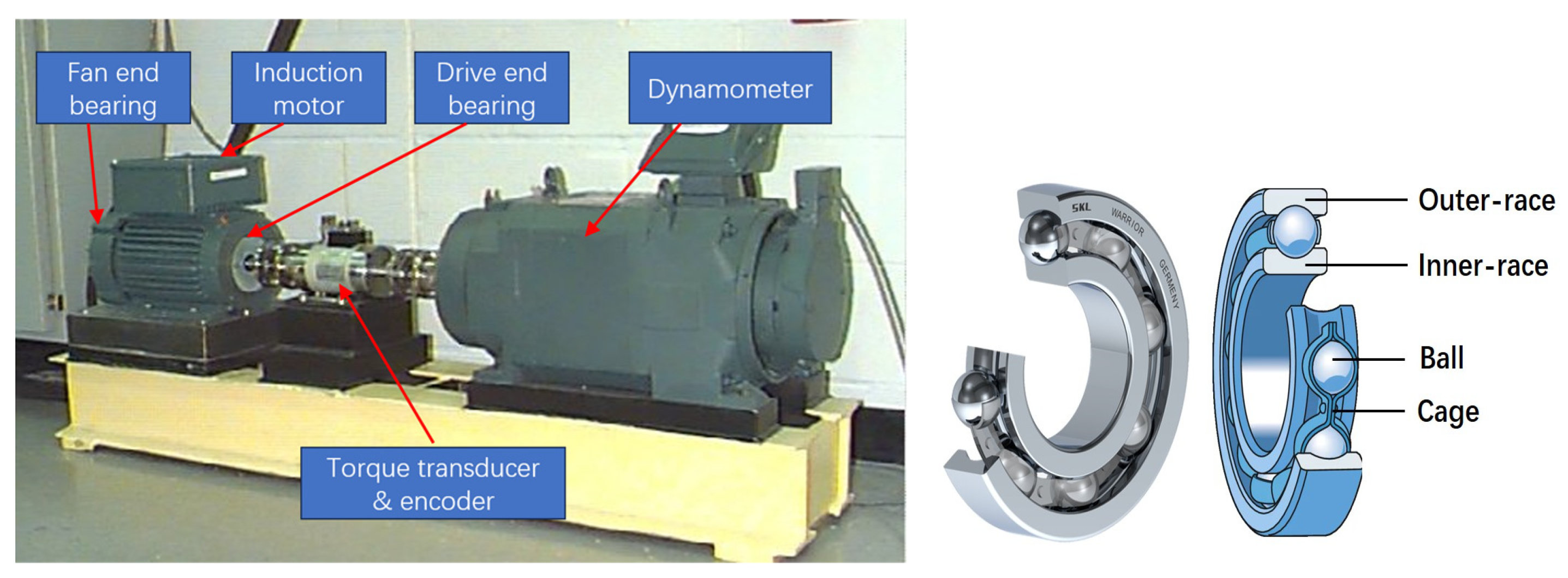
The Case Western Reserve University (CWRU) bearing fault dataset is widely used in the field of fault diagnosis for comparing the performance of different algorithms. As shown in Figure 8, the experimental setup consists of four components: a 1.5 kW (2 horsepower) electric motor, a torque sensor, a power meter, and an electronic controller.

The experimental motor operates with a load of 0 horsepower and an approximate speed of 1792 rpm, with a sampling frequency of 48 kHz. The vibration signals collected from the drive-end bearing housing are categorized into 10 fault modes: normal, inner race, outer race, and rolling element, with fault diameters of 0.1778 mm, 0.3556 mm, and 0.5334 mm, and a fault depth of 0.2794 mm. The fault data are represented as N, I1, I2, I3, O1, O2, O3, B1, B2, and B3. Among them, N represents normal; I denotes inner race surface faults; O indicates outer race surface faults; B represents rolling element faults; and 1, 2, and 3 correspond to fault diameters of 0.1778 mm, 0.3556 mm, and 0.5334 mm, respectively. The bearing fault data sample information is shown in

Table 1. CWRU fault data sample information.

Fault Location	Fault Diameter/mm	Training/Validation/Testing Samples	Label
Normal	-	350/100/50	N
Inner ring	0.1778	350/100/50	I1
Inner ring	0.3556	350/100/50	I2
Inner ring	0.5334	350/100/50	I3
Outer ring	0.1778	350/100/50	O1
Outer ring	0.3556	350/100/50	O2
Outer ring	0.5334	350/100/50	O3
Rolling element	0.1778	350/100/50	B1
Rolling element	0.3556	350/100/50	B2
Rolling element	0.5334	350/100/50	B3

.

The bearing model used for the drive-end in the experiment is the 6205-2RS JEM SKF deep groove ball bearing, with parameters shown in

Table 2. Parameters of the rolling bearing SKF6205.

Rolling Diameter/mm	Pitch Diameter/mm	Rolling Body Number	Contact Angle/°
7.94	39.04	9	0

. The fault characteristic frequencies of the bearing are calculated and presented in

Table 3. Fault characteristic frequency of the rolling bearing SKF6205.

	Inner Ring	Outer Ring	Rolling Element	Cage
Characteristic frequency/Hz	161.58	107.22	140.67	11.95
Characteristic period/s	0.0062	0.0093	0.0071	0.0837

.

3.1.2. FFT Result

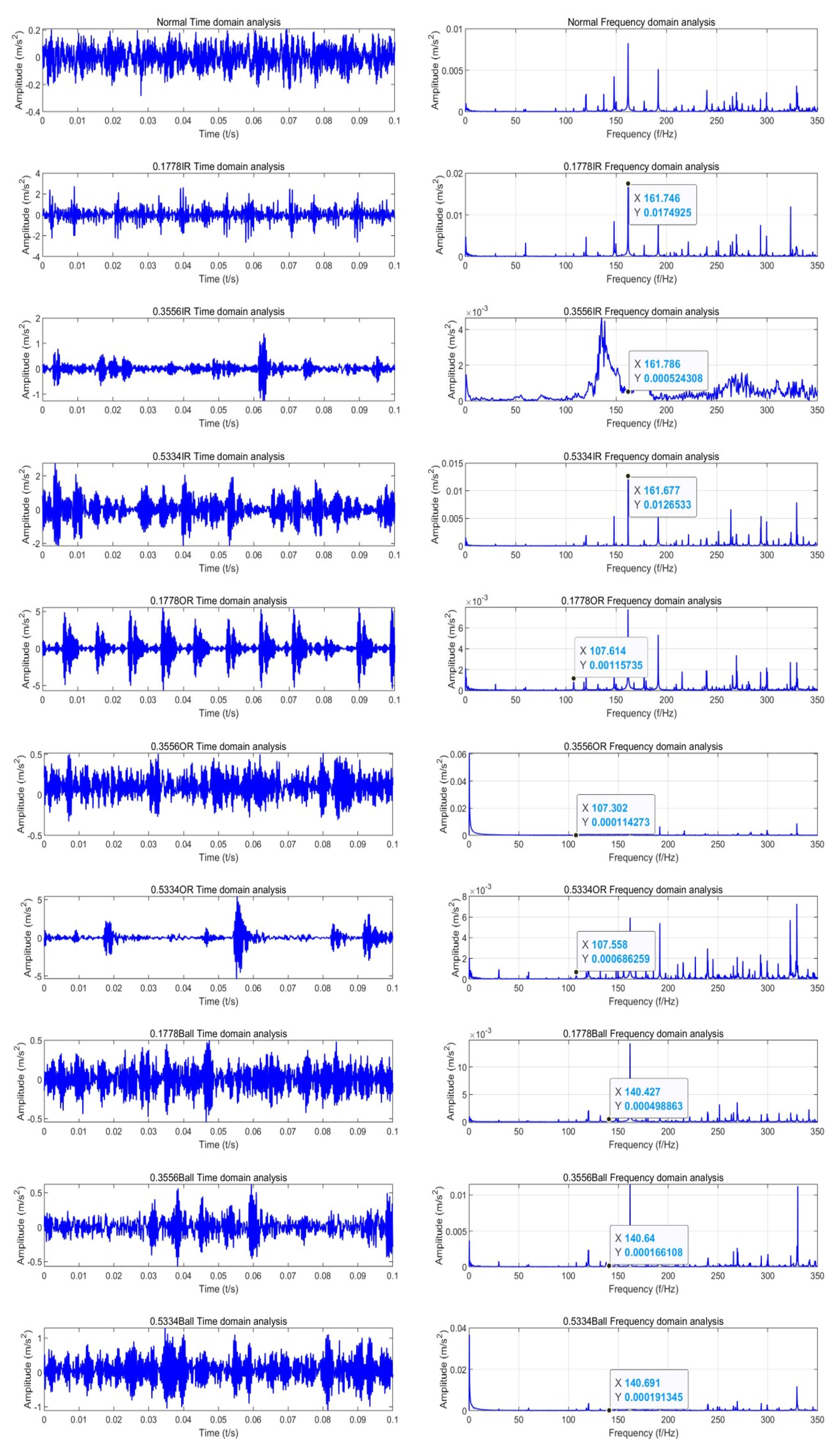
Figure 9 shows the time-domain waveforms of the bearing vibration signals collected under normal and nine fault conditions, along with the corresponding frequency spectra obtained after signal preprocessing using FFT.

On the left, the time-domain waveforms represent the bearing signals over a 0.1 s interval. Compared to the normal condition, when a fault occurs in a specific component, the time-domain waveform exhibits noticeable periodic variations. By observing for abnormal impacts or vibrations, it is possible to indicate the presence of a fault in the bearing. However, the time-domain signal is prone to noise interference, which can distort the waveform and affect the accuracy of fault diagnosis. On the right, the frequency spectrum after FFT processing is presented. In the normal condition, the characteristic frequencies of each component can be identified. When a fault occurs in a component, the fault can be determined based on the frequency value. Additionally, the magnitude of the signal at each frequency can help further assess the extent of the damage to the component. Noise in the time-domain signal is converted to low-value components in the frequency domain, which helps to suppress the noise.

As shown on the right, fault characteristic frequencies of 161 Hz, 107 Hz, and 140 Hz are identified in the frequency domain, corresponding to faults in the bearing’s inner race, outer race, and rolling elements. Based on the amplitude values of the frequency domain signals at 161 Hz—0.0174, 0.0005, and 0.0126, the fault diameters can be determined as 0.1778 mm, 0.3556 mm, and 0.5334 mm, respectively. Compared to the time-domain waveform, the frequency spectrum makes it easier to identify the fault location and severity and facilitates the extraction of sequence features.

3.1.3. Model Analysis

To verify the effectiveness and diagnostic performance of the proposed FFT-SE-TCN-SVM method, it is compared with FFT-TCN and FFT-SE-TCN in the experiments. CWRU bearing fault data are used, with each sample consisting of 1024 data points. For each type of fault, 500 experimental samples are randomly selected for model testing and comparison.

Faults in the diagnostic model involve numerous hyperparameters, but experiments show that fine-tuning these hyperparameters has little effect on the overall diagnostic performance of the model. Therefore, this paper does not analyze the impact of hyperparameters.

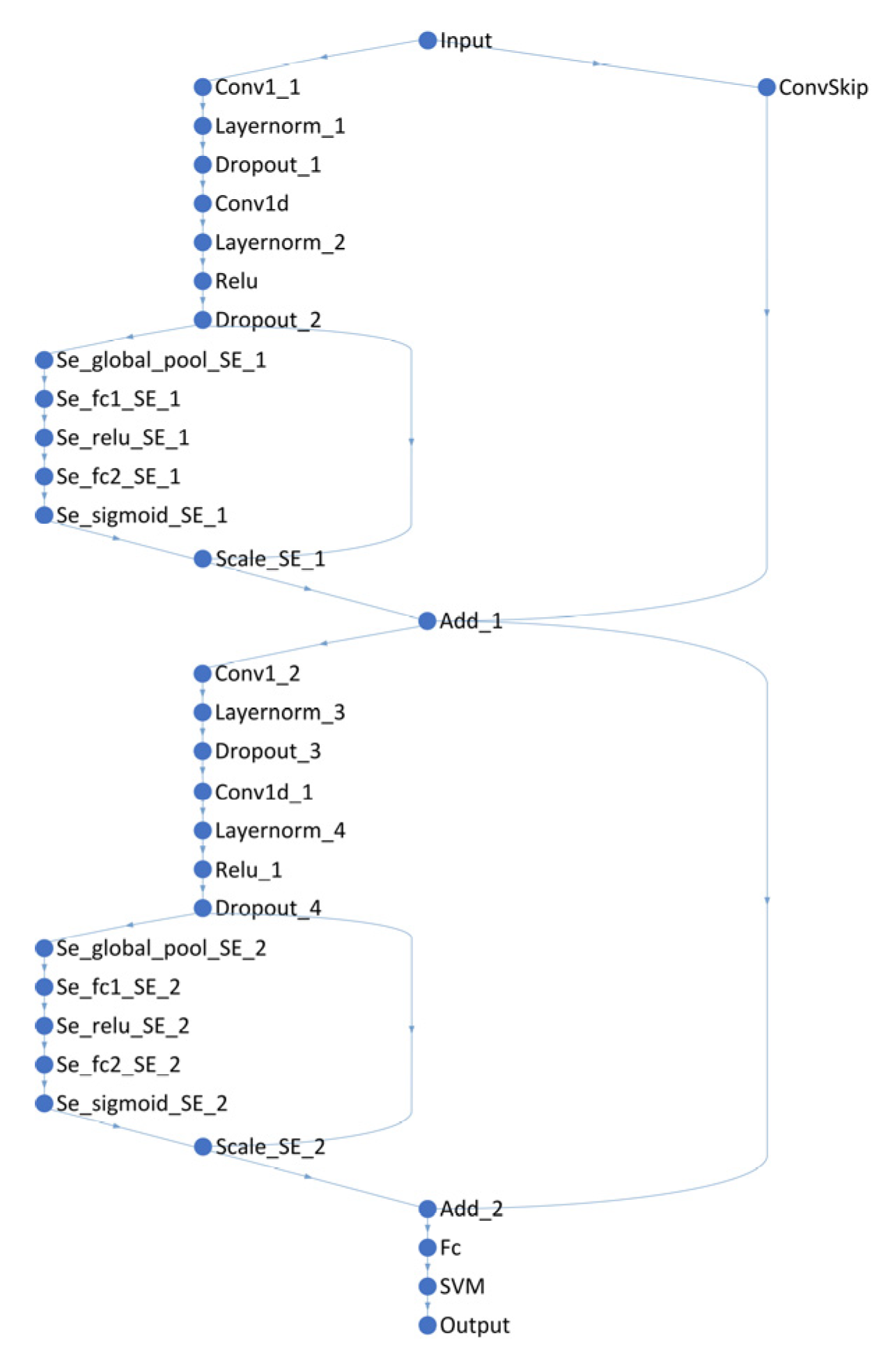
To enable adaptive learning rates and parameter updates in the negative gradient direction for faster network convergence, the TCN model employs the Adam optimizer. Additionally, to better capture the nonlinear features in the data, the Leaky ReLU activation function is selected. The maximum number of iterations is set to 50. The hyperparameter settings for the TCN model are listed in

Table 4. TCN model hyperparameter setting.

Model Hyperparameter	Parameter Setting	Model Hyperparameter	Parameter Setting
Optimization algorithm	Adam	Activation function	Leaky ReLU
Loss function	categorical cross entropy	Expansion factor	1, 2
Number of convolution kernel	16	Convolution kernel size	3
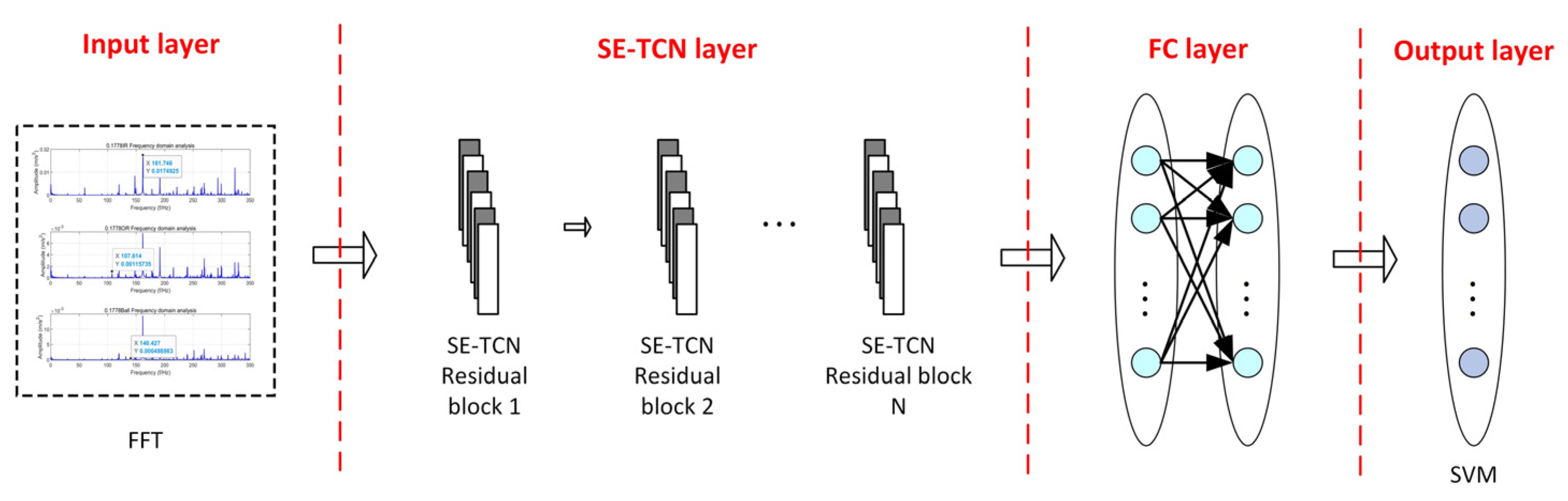
Random inactivation factor	0.2	Learning rate	0.001

. The article sets up 2 SE-TCN modules, and the network structure is shown in Figure 10.

After determining the structure of the SE-TCN model, TCN is combined with SVM. The RBF (radial basis function) kernel is chosen for the SVM, as it can model nonlinear responses and has fewer parameters than polynomial functions, significantly reducing the algorithm’s dependence on computational resources and providing a foundation for the algorithm’s real-time performance. The SVM parameters, including the penalty factor C and kernel parameter g, are optimized using the Particle Swarm Optimization (PSO) algorithm to obtain the optimal fault classifier.

Three models—FFT-TCN, FFT-SE-TCN, and FFT-SE-TCN-SVM—were constructed for testing and comparative analysis. To enhance the reliability of the experimental results, each method was tested 10 times, and the average of the 10 trials was used as the performance metric for classification evaluation, as shown in

Table 5. Model evaluation index for CWRU data.

Evaluation Index	FFT-TCN	FFT-SE-TCN	FFT-SE-TCN-SVM
Training duration/s	110.500069	143.996246	143.046461
F1 score	0.8855	0.8964	0.9073
Recall	0.8696	0.8804	0.8911
Accuracy rate	97.4%	98.6%	99.8%

. The results of a particular training session are depicted in Figure 11 and Figure 12.

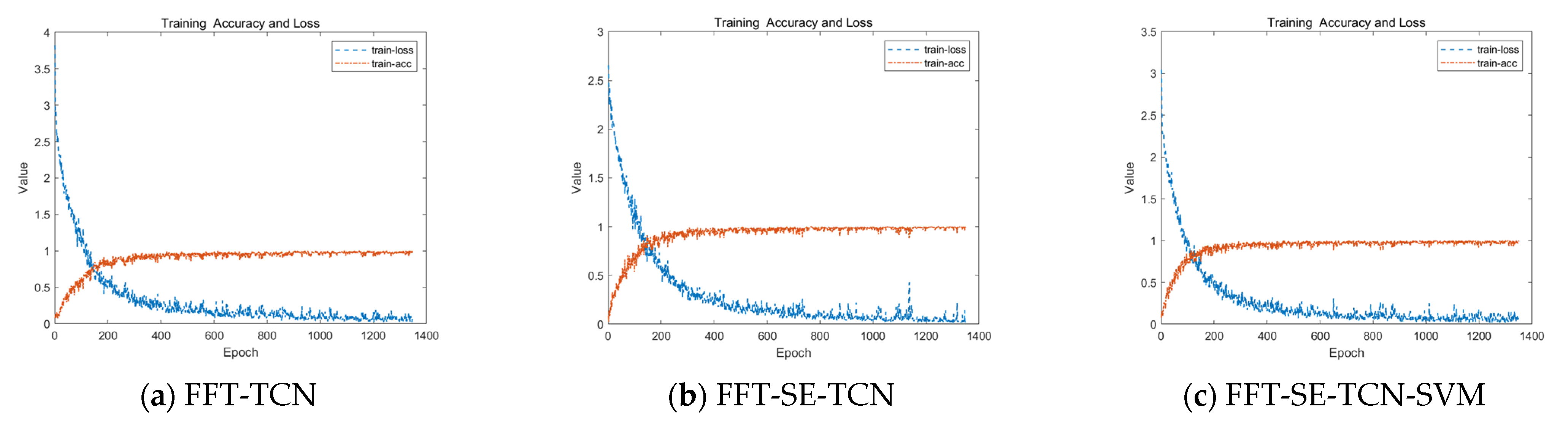
From Figure 11, it can be observed that as the algorithm continues to train, all three methods gradually stabilize, and their classification accuracy improves accordingly. This indicates that the TCN-based architecture exhibits strong stability in fault detection, highlighting the scientific significance of research focused on improving this foundational module. With the introduction of the attention mechanism, there is more fluctuation in classification accuracy during the early stages of training compared to the previous methods. This is because the attention mechanism is designed to mitigate the computational resource consumption associated with exhaustive search strategies based on sliding windows. In the early stages of training, the algorithm may lack sufficient knowledge accumulation, leading to missed signals in regions that should have been prioritized, resulting in false negatives.

However, as shown in the latter part of the waveform, after complete data training, the stability of the classification accuracy, particularly with the attention mechanism-based training strategy, is significantly improved. In comparison, the specific data in Figure 12 demonstrate that the FFT-SE-TCN-SVM network structure proposed in this paper has a substantial advantage in terms of classification accuracy.

The test results were analyzed in detail using confusion matrices, which provide a more intuitive view of the fault detection performance for various bearing faults in the test set. (a) The FFT-TCN model achieved a diagnostic accuracy of 97.4%, with a misclassification rate of 22.9% for normal bearing data being incorrectly identified as a 0.1778mm inner race fault. (b) The FFT-SE-TCN model achieved a diagnostic accuracy of 98.6%, with the primary misclassification occurring when a 0.1778mm inner race fault was incorrectly classified as a normal state, with a fault rate of 13%. (c) The FFT-SE-TCN-SVM model correctly classified both the normal state and the 0.1778mm inner race fault. All three models showed varying degrees of misclassification for the 0.3556mm rolling element fault, with no significant differences observed.

In addition to the confusion matrix, the models were compared using training time, F1 score, recall, and accuracy metrics, as shown in Table 5. The table reveals that the classification accuracy of all three models reached over 97%, with overall good performance. However, the FFT-SE-TCN-SVM network showed improvements in F1 score, recall, and accuracy compared to the FFT-TCN and FFT-SE-TCN models. Specifically, the accuracy reached 99.8%, an increase of 2.4% and 1.2% over the other two networks, indicating the best overall model performance. The recall was 0.8911, improving by 2.15% and 1.07%, which indicates a stronger ability to correctly identify positive samples and a lower false negative rate. The F1 score was 0.9073, improving by 2.18% and 1.09%, suggesting that the model performs well in both precision and recall, effectively identifying positive samples while minimizing false positives.

However, the training time increased by 33.49 s when the SE module was added to the TCN network. Given that the SE module enhances the feature extraction ability of the model by selecting key channels through nonlinear transformations, the additional computational cost associated with the SE module is considered acceptable due to the improvement in model performance. The experimental results show that the execution time of FFT-SE-TCN-SVM is shorter than that of FFT-SE-TCN. This can be attributed to two factors. First, TCN requires iterative optimization of all parameters during end-to-end training, and as the input signal length or network depth increases, the complexity of gradient calculation during backpropagation grows exponentially. In contrast, FFT-SE-TCN-SVM separates feature learning (FFT-SE-TCN) from classification decision (SVM), reducing the training complexity. Second, if PSO detects that the fitness fluctuates less than 1% for five consecutive iterations, it terminates early, avoiding redundant calculations. This makes the latter, although more complex, able to perform the optimization process more quickly.

In summary, the proposed method demonstrates significant advantages in terms of F1 score, recall, and accuracy, with a classification accuracy of 99.8%. This is considered a high classification accuracy in the field of AI-based recognition, indicating a clear superiority of the proposed method. It is important to note that compared to the FFT-TCN model, the latter two methods do not offer an advantage in training time. However, this refers to the training time of the algorithm, not the time consumed during its application. The time difference is associated with the computational cost during the model’s training process, rather than the processing time required during actual application. Therefore, the impact on the algorithm’s real-world application is minimal. When mechanical faults occur, the duration of such faults is typically longer, and the accuracy of fault diagnosis is generally more critical than the processing time.

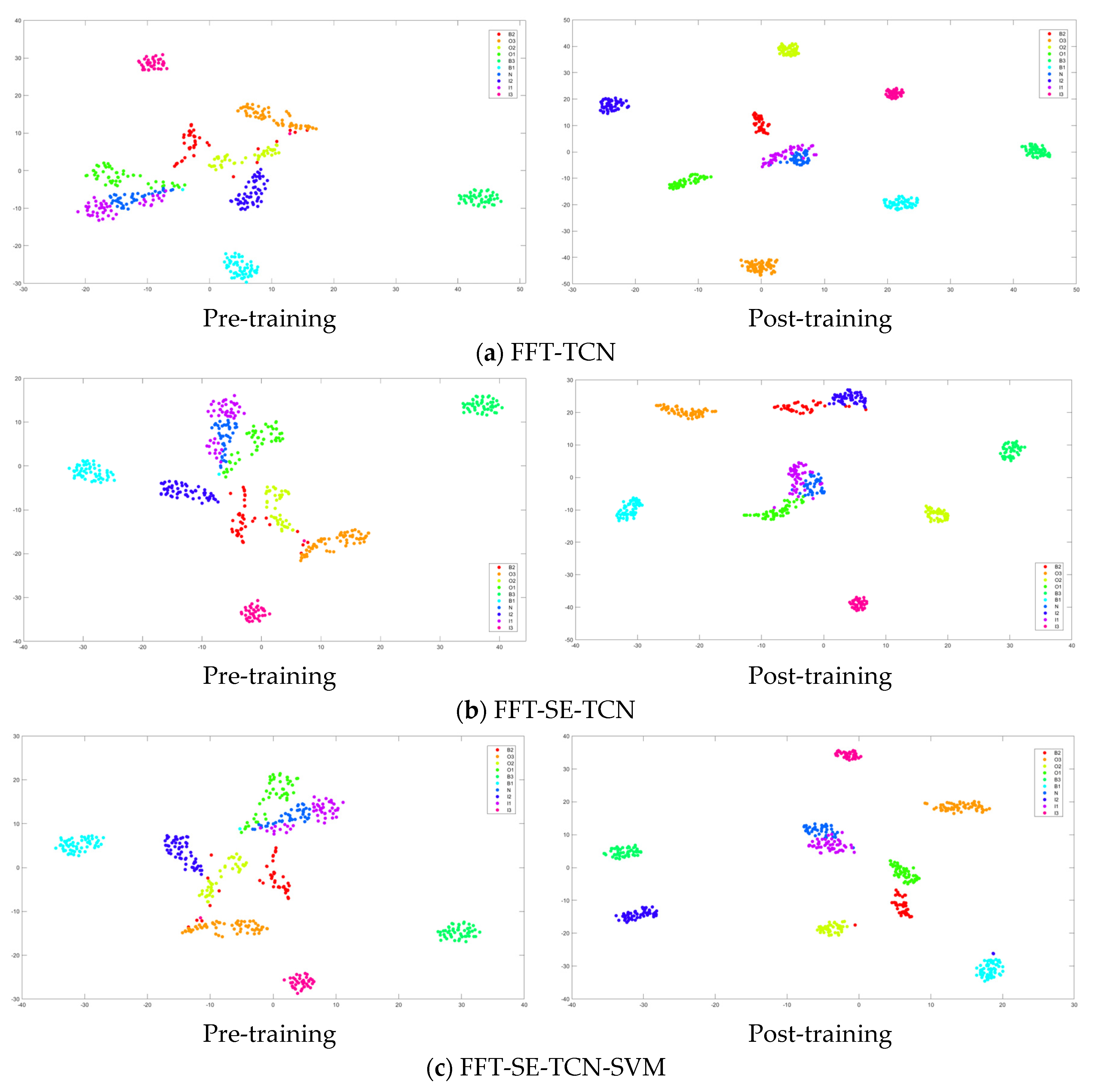
3.1.4. T-SNE Visual Analysis

To further evaluate the feature learning ability of the improved FFT-SE-TCN-SVM model and visually demonstrate its effect on feature extraction from input data, t-Distributed Stochastic Neighbor Embedding (t-SNE) was used to map the high-dimensional feature space onto a two-dimensional plane for visualization. This method effectively preserves local structures, ensuring that similar data points remain close to each other in the low-dimensional space, which is useful for understanding the internal structure of complex datasets.

Figure 13 presents the fault feature visualization results after dimensionality reduction using t-SNE, with a comparison between the outputs before and after applying the three models. As shown in the figure, all three models are able to achieve a certain degree of fault feature separation, but there are significant differences in terms of clarity and clustering performance. The proposed improved model exhibits more distinct fault feature boundaries, with greater distances between different categories, indicating stronger discriminative ability and better generalization performance.

The experimental results demonstrate that the proposed method effectively extracts the raw fault features from the input data and transforms them into more representative features that better capture the essence of the faults, making it highly effective for bearing fault diagnosis and classification.

3.2. Experimental Analysis of Small Sample Data

In practical industrial environments, obtaining a large number of labeled bearing fault samples is often very challenging, making small-sample data testing a highly difficult task. To evaluate the proposed method’s diagnostic performance on small sample data, 50 samples were selected from each fault mode, totaling 500 samples, for training and testing the model to validate its effectiveness.

The model was trained with the same hyperparameter settings as in Section 3.1. Cross-validation was used to reduce bias caused by randomness. Each method was tested in 10 experiments, and the average results of these 10 trials were taken as the classification performance metric. The results are shown in

Table 6. Model evaluation index for small sample data.

Evaluation Index	FFT-TCN	FFT-SE-TCN	FFT-SE-TCN-SVM
Training duration/s	10.995200	19.920746	17.399811
F1 score	0.8373	0.8472	0.8697
Recall	0.7625	0.8164	0.9038
Accuracy rate	85.4%	89.8%	92.4%

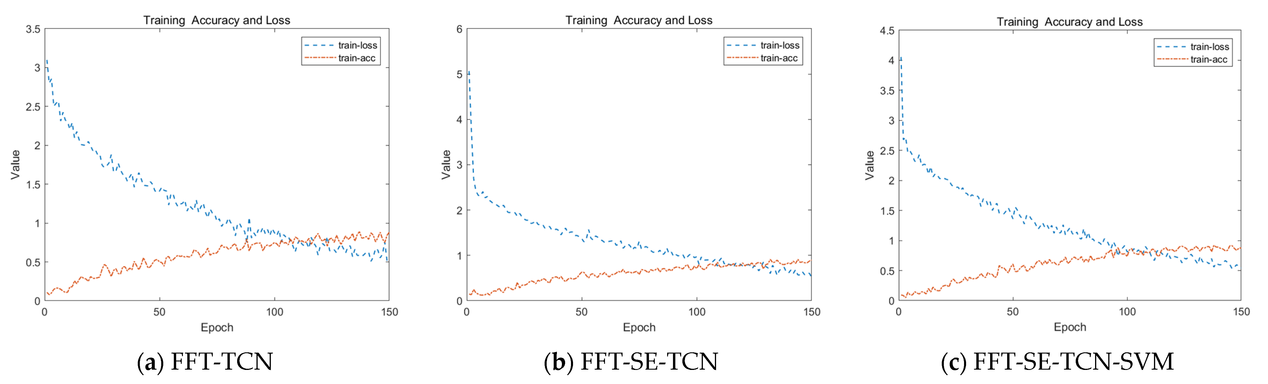
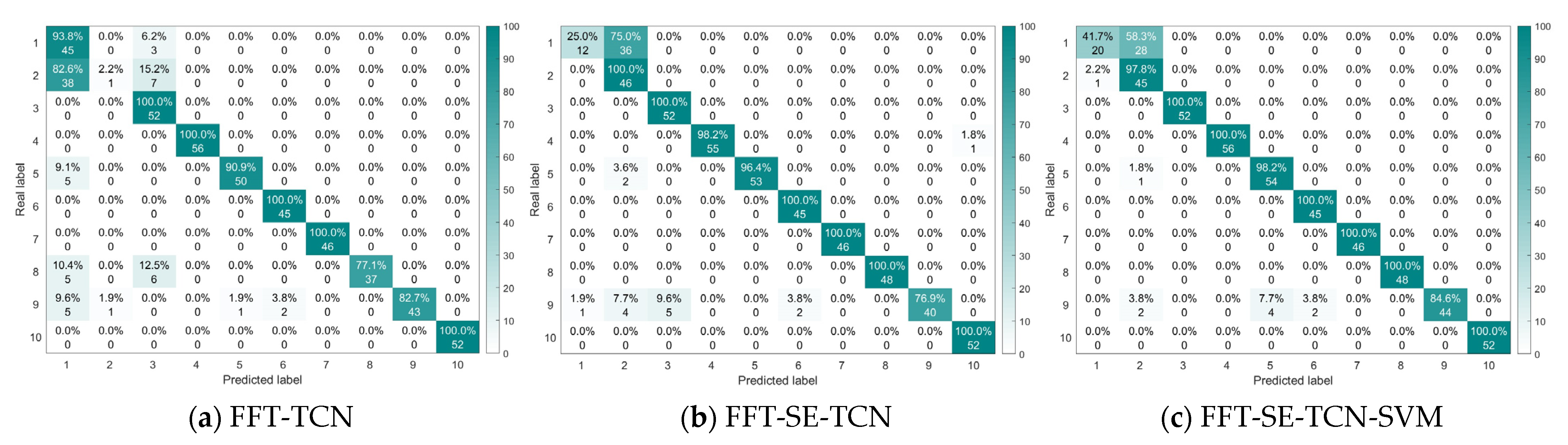
, and Figure 14 and Figure 15 illustrate the classification results from a particular training session.

Figure 14 shows the training accuracy and loss curves for the three models. As the number of training epochs increased, the training accuracy gradually improved. The FFT-TCN model’s training loss decreased steadily, while the training losses of the FFT-SE-TCN and FFT-SE-TCN-SVM models dropped rapidly at first and then leveled off. The curves for the latter two models were smoother, indicating that the SE mechanism effectively enhanced the learning efficiency of the models. However, due to the limited data under the small sample condition, the training results had not stabilized after 150 training epochs. Therefore, in small-sample data conditions, adjusting the batch size to make gradient updates more stable could help achieve a more stable training process.

Figure 15 shows the confusion matrix for the classification results of the three models. The FFT-TCN model achieved an accuracy of 85.4%, but the classification accuracy for the 0.1778 mm inner race fault was only 2.2%, and the classification results for the 0.1778 mm and 0.3556 mm rolling element faults were relatively poor. The FFT-SE-TCN model achieved an accuracy of 89.8%, but the false positive rate for the bearing’s normal state was as high as 75%, and the classification accuracy for the 0.3556 mm rolling element fault was only 76.9%. The FFT-SE-TCN-SVM model similarly showed lower accuracy for the normal bearing state and the 0.3556 mm rolling element fault, but overall, it outperformed FFT-SE-TCN with an accuracy of 92.4%.

Table 6 compares the training time, F1 score, recall, and accuracy metrics for the three models. The proposed method does not have an advantage in training time but performs better overall in the other three evaluation metrics.

As shown in the fault feature visualization results of Figure 16, none of the three models could effectively cluster and separate the normal bearing state and the 0.1778 mm inner race fault. The FFT-TCN model performed relatively better.

In summary, the proposed method demonstrates better overall fault classification performance for small sample data. To address the issue of insufficient fault data samples, data augmentation techniques can be applied to generate more diverse training samples, helping the model achieve better generalization.

3.3. Evaluation of the Model Generalization Ability

To evaluate the learning capability of the model proposed in this paper for unseen data, bearing fault data collected in the laboratory were used for testing and validation. This process aims not only to assess whether the model can extract generalizable patterns from the limited training samples but also to ensure that it maintains good predictive performance on previously unseen data.

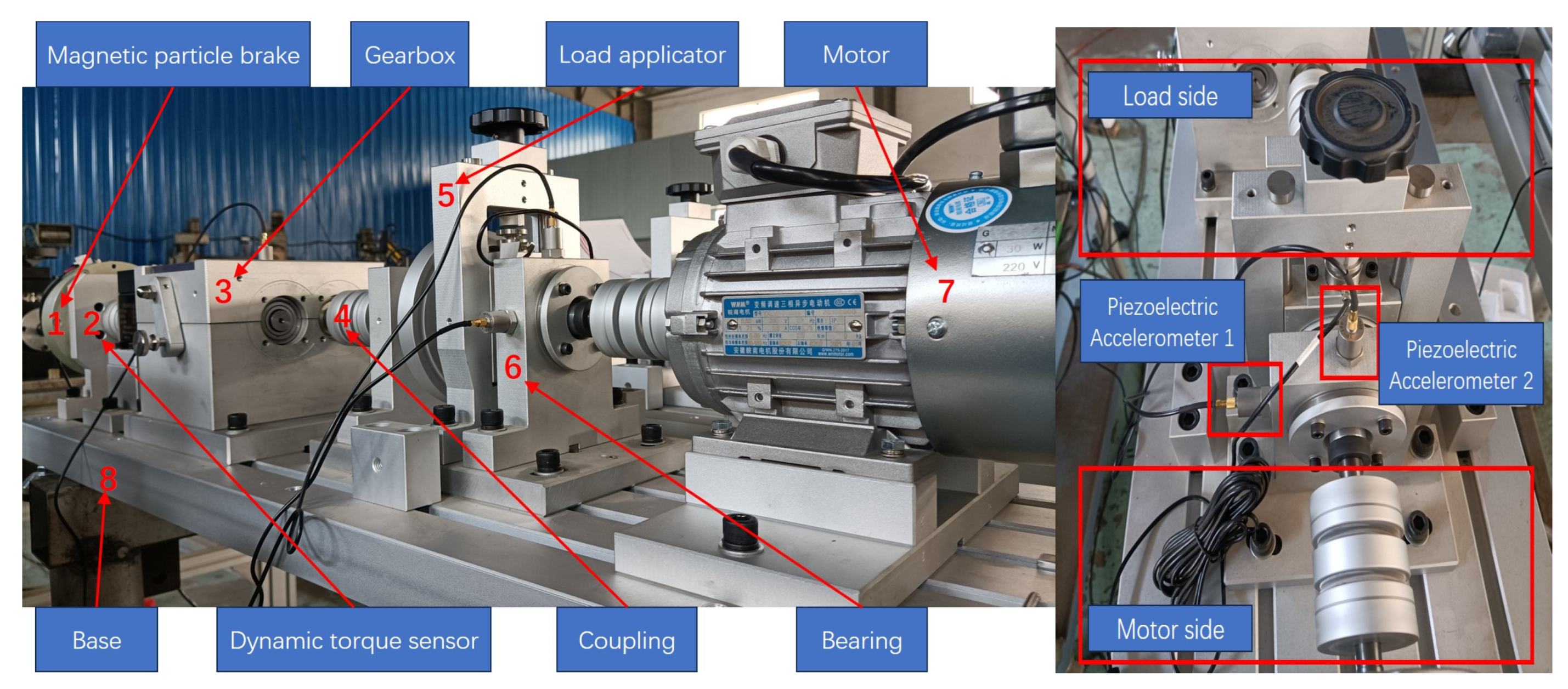
3.3.1. Data Set Introduction

The HFDZ-330 rotating machinery fault implantation experimental platform, built in the laboratory, is shown in Figure 17. The experiment utilized three YD-186 piezoelectric accelerometers to collect vibration signals, which were installed at the longitudinal direction of the load side gearbox, the horizontal direction of the motor-side bearing, and the longitudinal direction of the bearing, with a sampling frequency of 51,200 Hz. The bearings were tested under operating conditions of 1500 r/min and 2100 r/min, with three different load conditions: no load, medium load of 10 kg, and high load of 20 kg. Additionally, a speed-up process from 0 to 2100 r/min was set up to simulate non-stationary operating conditions with varying speeds.

The experimental bearings used were of the model 6203-2Z SKF, with parameters listed in

Table 7. Parameters of rolling bearing SKF6203.

Rolling Diameter/mm	Pitch Diameter/mm	Rolling Body Number	Contact Angle/°
7	35	9	0

. The characteristic frequencies for a rotational speed of 1500 r/min are provided in

Table 8. Fault characteristic frequency of rolling bearing SKF6203.

	Inner Ring	Outer Ring	Rolling Element	Cage
Characteristic frequency/Hz	123.75	76.25	99.75	9.50
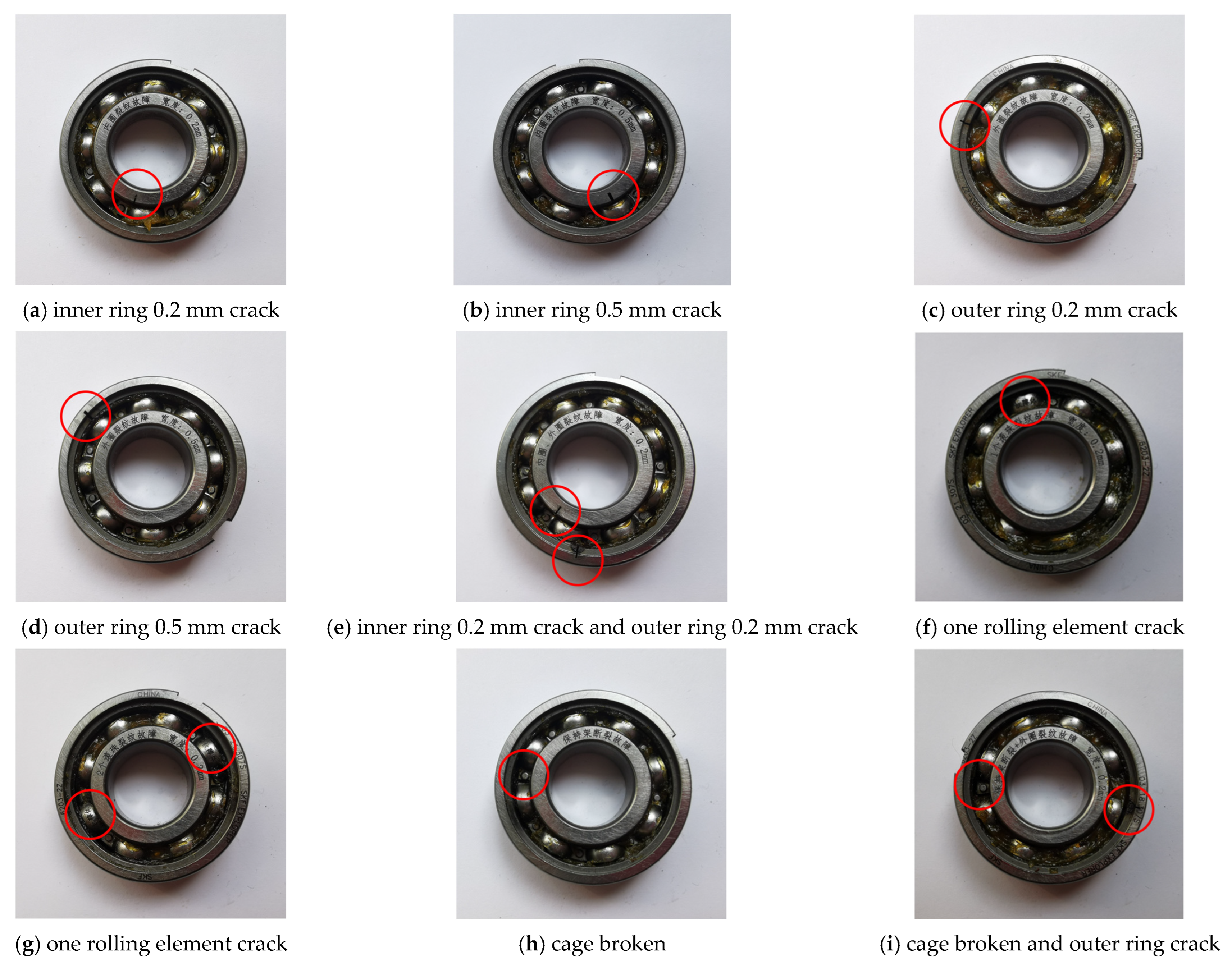
Characteristic period/s	0.0081	0.0131	0.0101	0.1053

. Prior to the experiment, grooves of varying degrees of damage were machined on the inner ring, outer ring, rolling elements, and cage using wire electrical discharge machining, as shown in Figure 18. The red circles highlight the fault locations.

The experiment was arranged under a rotational speed of 1500 r/min and a load of 10 kg, with 10 fault modes, including normal state, inner ring crack with a width of 0.2 mm, inner ring crack with a width of 0.5 mm, outer ring crack with a width of 0.2 mm, outer ring crack with a width of 0.5 mm, inner and outer ring cracks with a width of 0.2 mm, one ball crack with a width of 0.2 mm, two ball cracks with a width of 0.2 mm, cage fracture fault, and composite outer ring crack fault with a width of 0.2 mm. The bearing fault data sample information is presented in

Table 9. Fault data sample information.

Fault Location	Fault Diameter/mm	Testing Samples	Label
Normal	-	50	N
Inner ring crack	0.2	50	I0.2
Inner ring crack	0.5	50	I0.5
Outer ring crack	0.2	50	O0.2
Outer ring crack	0.5	50	O0.5
inner and outer ring cracks	0.2	50	IO
one ball crack	0.2	50	B1
two ball cracks	0.2	50	B2
cage fracture fault	-	50	C
cage fracture fault composite outer ring crack fault	0.2	50	CO

, which includes not only single fault types but also data on various compound fault types. By using a high-quality and diverse dataset, this allows for a more accurate evaluation of the model’s performance when faced with complex and variable real-world application scenarios.

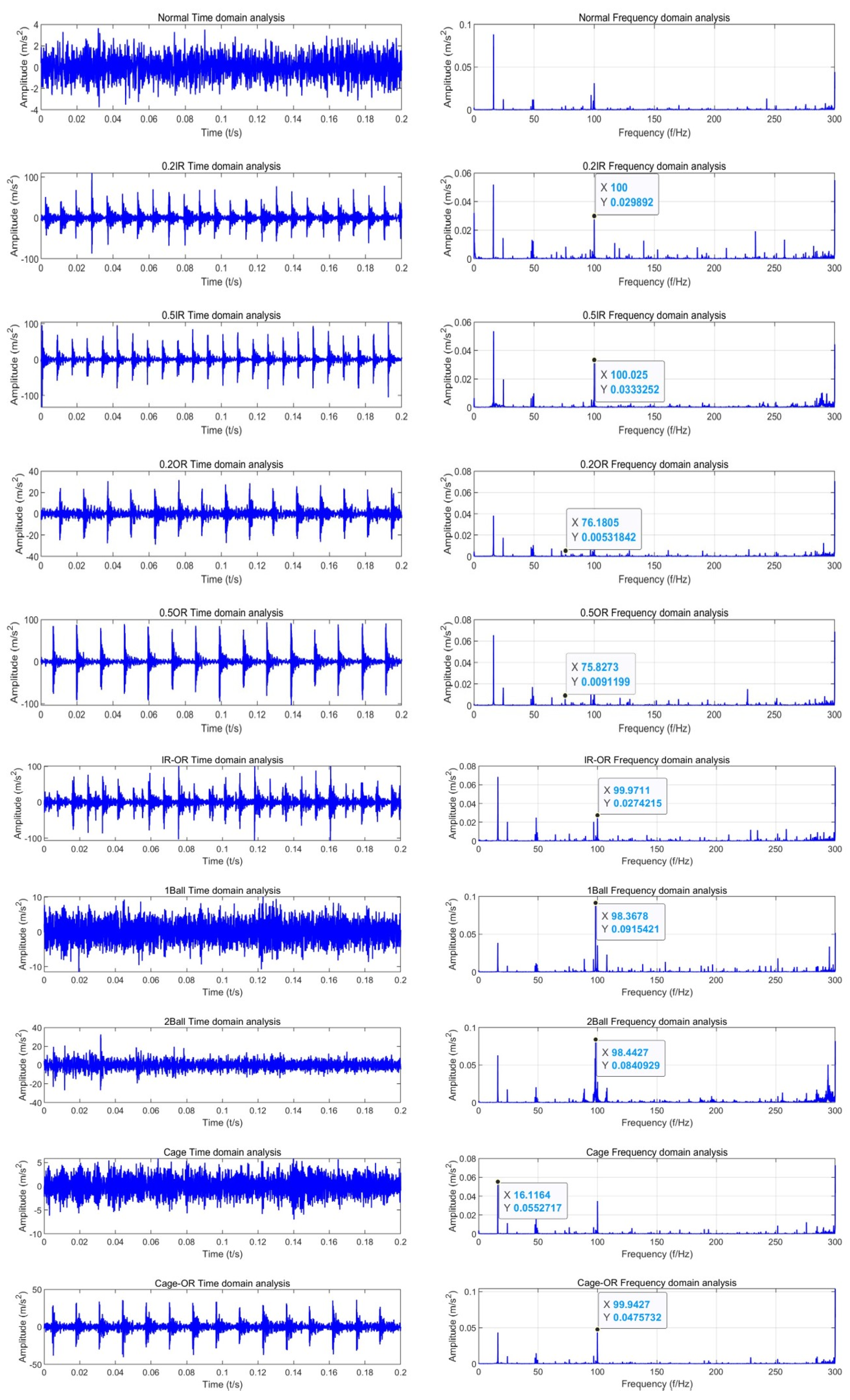
3.3.2. FFT Result of Laboratory Data

Figure 19 shows the time-domain and frequency–domain analysis results of normal and faulty bearing data collected in the laboratory.

In the normal state, the time-domain signal of the bearing vibration is relatively stable, with no obvious periodic fluctuations or abnormal peaks. The frequency spectrum is smooth, with the main energy concentrated in the low-frequency range. In the faulty state, the time-domain signal exhibits periodic pulse signals, indicating the presence of some periodic impact or vibration. For different faults, the amplitude and pulse interval of the pulse signal change. After applying FFT to process the signal, specific frequency components caused by the fault appear as prominent peaks in the frequency–domain plot. The inner race fault is found around 100 Hz, with fault diameters of 0.2 mm and 0.5 mm corresponding to amplitudes of 0.0298 and 0.0333 m/s², respectively. The outer race fault frequency peak appears at 76 Hz, with fault diameters of 0.2 mm and 0.5 mm corresponding to amplitudes of 0.0053 and 0.0091 m/s², respectively. Therefore, the frequency–domain data obtained from the FFT processing of the collected signal are more conducive to extracting sequential information and assisting in subsequent analysis.

3.3.3. Model Analysis of Laboratory Data

To verify the generalization ability of the proposed FFT-SE-TCN-SVM method for bearing fault data collected on the laboratory platform, the network model trained on the CWRU bearing fault dataset is tested on the laboratory-collected bearing fault data. This is to examine whether the model can maintain good predictive performance on unseen new data.

The laboratory data are organized with 2048 points as one sample, and 50 samples are randomly selected for each type of fault to form the test set. The fault data sample information is shown in Table 9. The classification and diagnostic performance of the model based on the original sample data in Section 3.1 and the small sample data model in Section 3.2 are evaluated.

In this experiment, the model parameters are strictly frozen: the SE-TCN network weights and PSO-SVM hyperparameters are determined based on the CWRU dataset. The laboratory data are used only for forward inference testing and do not participate in any gradient updates or parameter optimization. Cross-validation is used to reduce bias caused by randomness. Ten experiments are conducted, and the average result of the ten trials is used as the performance metric for classification evaluation.

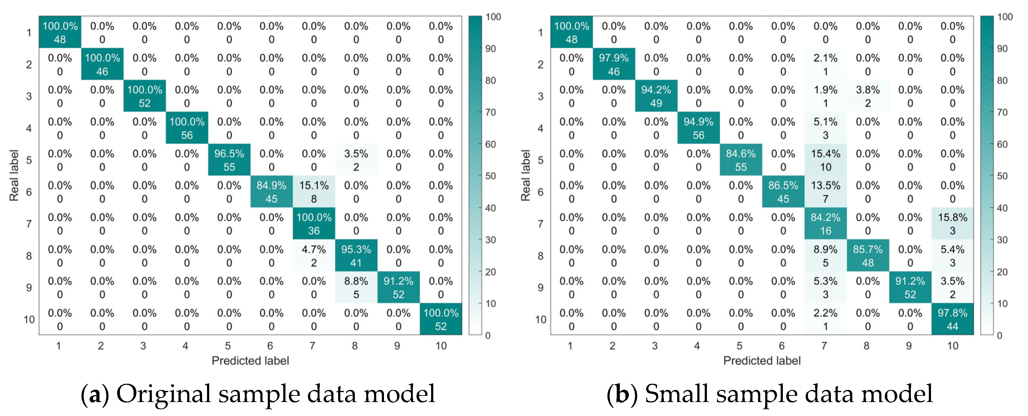
Figure 20 shows the confusion matrix of the classification results for the original sample data model and the small sample data model for a specific trial. In Figure 20a, the accuracy of the test set for the original samples reached 96.6%, with a small number of classification errors for the bearing faults including a 0.5 mm outer ring crack, 0.2 mm inner and outer ring cracks, 0.2 mm cracks in two rolling elements, and cage fracture. All other faults were classified correctly. In Figure 20b, the accuracy for the small sample test set reached 91.8%, with correct classification only for the normal bearing state, and varying degrees of classification errors for all fault states.

The test results show that the proposed model achieves good diagnostic performance on laboratory bearing fault data, with a high average fault classification accuracy, demonstrating strong generalization ability.

4. Conclusions

In response to the challenges posed by the strong nonlinearity and temporal characteristics of rolling bearing fault data, as well as the inaccuracies of fault diagnosis relying on human experience, this paper proposes an intelligent fault diagnosis method based on FFT, SE-TCN, and SVM. The method effectively detects and diagnoses rolling bearing faults. By comparing it with two other network structures, FFT-TCN and FFT-SE-TCN, the results demonstrate the advantages of the proposed algorithm in fault detection and diagnosis of rolling bearings.

The experimental results show the following:

• Using FFT as the data preprocessing step for bearing fault vibration signals can reduce dimensionality and denoise the original signal, highlighting key frequency components. This allows the TCN to more easily capture critical features, thereby improving diagnostic accuracy. The TCN model is further enhanced by incorporating the attention mechanism from SENet, which strengthens the model’s feature extraction ability and improves feature representation;
• Replacing the Softmax classifier with an SVM classifier and optimizing its parameters using Particle Swarm Optimization (PSO) takes advantage of the SVM’s ability to handle small sample sizes and nonlinear problems. This addresses the limitations of Softmax in dealing with nonlinear issues and further improves the network’s classification performance. However, the factors affecting the performance parameters of SVM, such as data volume and sample frequency, need further analysis and verification;
• The proposed method achieves high diagnostic accuracy and good generalization ability, overcoming the limitations of traditional methods that require manual feature preprocessing. It holds practical value in the era of big data. However, due to limited data samples, the study is focused solely on bearing fault data. The model has not yet been tested on fault vibration data from other rotating machinery, such as bearings and gearboxes, outside of the acquired database. In future research, the author plans to obtain more rolling bearing fault data samples to further validate the effectiveness of the proposed diagnostic method;
• In this study, we only analyzed fault data under stable operation of mechanical equipment, specifically under constant speed conditions. In practical applications, the working speed of the equipment may change, which can affect the performance of fault diagnosis. Therefore, fault features under traditional fixed speed conditions may not be applicable under variable speed conditions. Whether the proposed solution can be effectively applied in this scenario requires further analysis. Additionally, in practical applications, the proposed solution involves multiple steps and relatively complex algorithms, which results in higher computational costs and needs further validation.